Reliability Assessment of Integrated Power and Road System for Decarbonizing Heavy-Duty Vehicles

Abstract

With the continual expansion of urban road networks and global commitments to net zero, electric vehicles (EVs) have been considered to be the most viable solution to decarbonize the transportation sector. In recent years, the electric road system (ERS) has been introduced and piloted in a few countries and regions to decarbonize heavy-duty vehicles. However, little research has been carried out on its reliability. This paper fills the gap and investigates the reliability of electric truck power supply systems for electric road (ETPSS–ER), which considers both the power system and truck traffic networks. First, a brief introduction of electric roads illustrates the working principle of EV charging on roads. Then, an optimized electric truck (ET) travel pattern model is built, based on which the corresponding ET charging load demand, including both static charging and dynamic charging, is conducted. Then, based on the new ET travel pattern model, a daily travel-pattern-driven Monte Carlo simulation-based reliability assessment method for ETPSS–ER system is presented. Case studies based on the IEEE RBTS system shows that ETs driving on ERS systems can meet the daily travel demands. The case studies also examine the impacts of increasing number of ETs, extra wind power, and battery energy storage systems (BESS) on the reliability of ERS power systems.

1. Introduction

Over the past few decades, transportation electrification has become a global trend. It can not only significantly decrease the enormous carbon emissions in the transport sector, but can also reduce the consumption of the limited fossil fuel reserves that can be used for other sectors. As of 2023, the transportation sector is still one of the largest contributors to greenhouse gas emissions responsible for the global climate change [1,2]. As 30% of railways have been electrified, road systems, which account for about 78% of $C{O}_2$ emissions in the transportation sector, have replaced railway (1%) as the most carbon-intensive means of transportation [3]. To address this problem, electric vehicles (EVs) have become the most viable solution to support future green-road systems [4]. Taking UK as an example, the proportion of newly registered EVs in 2022 reached 16.6%, representing an explosive yearly growth trend [5]. Up to date, about 7% of road vehicles in UK are electric, mainly including passenger vehicles and public buses [6]. Meanwhile, China, as a world front-runner, has more than half of the world on-road EVs, accounting for around 60% of global electric car sales. Meanwhile, in Europe, EV sales also increased by over 15% in 2022 [7]. Furthermore, to meet the net zero target by the middle of this century, freight vehicles, which account for about 25% of emissions from the road sector, also need to be electrified in order to cut down the total carbon emissions [3].

Although roll-out of electric trucks (ETs) is a potential solution for heavy-duty vehicles, there are still several limiting factors to be addressed [8]. Different from passenger vehicles, the heavy-load and long-distance features imply that ETs will not only need significantly large battery capacity, but will also demand higher-power charging devices, which will lead to a significant increase in capital and operational costs [9,10]. To address this bottleneck, an electric road system (ERS) that supplies dynamic charging power is considered to be a promising solution for future road decarbonization [11]. ERS is a newly emerging technology that can support vehicles charging while driving on the road via three different power supply solutions, namely, overhead line, conductive rail, and inductive (wireless power transfer) rail [12]. The first two modes are contact charging modes, which are exposed to external weather conditions, while wireless charging is a non-contact charging method, which may potentially make the charging smoother [13]. Therefore, this paper primarily focuses on the ETs driving on the ERS, which integrates dynamic and static charging to transmit electricity from the power grid to ETs.

To investigate the reliability of the ERS traction power supply system (TPSS) for ETs, it is necessary to understand their travel routes and charging patterns. Taking delivery ETs as an example, their total delivery distance depends on the travel route, which cannot exceed the total travel distance of fully charged ET batteries. Meanwhile, the arrival time and service time at each delivery point are both limited. Once the remaining battery capacity cannot support the ET to travel to the next service point, it needs to be recharged midway. This routine can be summarized as follows: ETs start at a fully charged state, may be recharged during the working hours, and return to the depot to be fully recharged at the end of the day. It is noted that the electric truck power supply system in electric road (ETPSS–ER) is a new research topic; little has been determined about its reliability, though some research has been carried out on the EV routing problem (EVRP) and the integration of EVs in the power system. For example, ref. [14] has proposed a load modeling approach for plug-in EVs, which can simulate different EV operation schedules, charging levels, and customer participation. Meanwhile, ref. [15] has considered several uncertainties and complex interdependencies of different factors associated to the load modeling of plug-in EVs. Furthermore, refs. [16,17,18] have discussed the vehicle-routing problem and proposed several methods to search for the most energy-efficient paths between any two nodes to be visited in the routes. In [19,20,21], an EV energy-consumption prediction model is built, considering the impacts of the traffic flow on the motor efficiency and driving resistances to improve the prediction accuracy. Further, in [22], an order-first split-second max–min ant system algorithm has been developed to generate routes that fulfill the demands of customers. And [23] has optimized the EV route selection with time window to achieve an economically viable solution. Inspired by these approaches, ET routing is introduced into the reliability study of the ETPSS–ER in this paper. The main contributions of this paper are summarized as follows.

• Based on the specific charging modes of the electric road system, the ET driving and charging patterns are defined and utilized to establish the interaction model between the electric road and the power supply system;
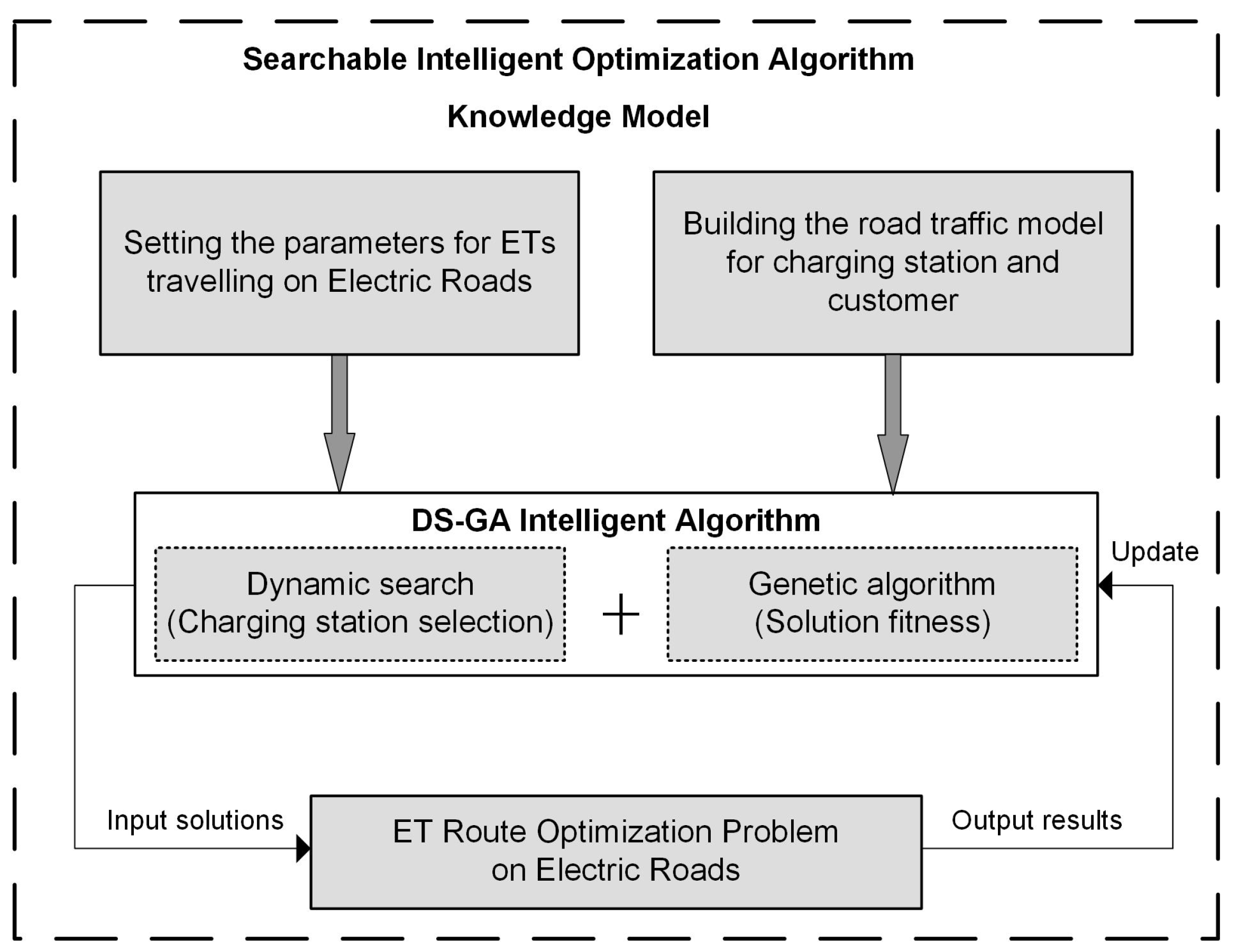
• In order to minimize the charging cost for ETs traveling on electric roads, an optimized routing-planning algorithm is developed. It integrates ET charging cost control with the routing planning, aiming to achieve the lowest charging cost while meeting all designated delivery tasks;
• Based on the optimized energy interaction model between the electric road and power supply system, a daily GA-driven Monte Carlo simulation-based reliability assessment method for ETPSS–ER system is proposed;
• A case study is conducted to assess the reliability of an integrated power and road system with different numbers of ET charging loads. It is shown that, in the case study, introducing the load of 1000 ETs will not cause major reliability concerns on the existing system, while, as the number of ETs exceeds 3000, it is necessary to introduce additional renewable power and BESS for more reliable ETPSS–ER system operation.

The remainder of the paper is organized as follows. Section 2 introduces the ET charging patterns and formulates the ET route optimization problem. Section 3 details the reliability assessment approach for the ETPSS–ER system. Section 4 presents the case studies and simulation results, and, finally, Section 5 concludes the paper.

2. Interaction Modeling between Electric Roads and Power Supply Systems

Electric trucks, as an emerging technology, can replace the traditional fossil fuel trucks to significantly reduce the carbon emissions in the road sector. To analyze the reliability of the ETPSS–ER, it is necessary to establish the energy interaction model between the power system and ERS with electric trucks. An ET traveling on the road has the following three power supply scenarios:

• Charging while traveling on ERS—ERS provides power to ET via dynamic wireless charging;
• ET is powered by the on-board battery while traveling on non-electric road;
• ET goes to a charging station to recharge the battery due to the energy shortfall before completion of the journey/task.

2.1. ET Charging Patterns

As elaborated earlier, the ET charging patterns can be summarized as below:

• Overnight charging (AC charging): When ETs are parked and charged overnight at depots, AC charging is the most common approach. This is usually a slow charging mode with the longest charging time and lowest cost [24];
• High-power charging at station (DC charging): Direct current charging stations are becoming more prevalent now for faster charging, which can shorten the charging time significantly. It covers various power levels from 40–350 kW with different charging tariffs [25];
• Pantograph charging (overhead line charging): Similar to DC railway or metro line traction power supply, ERS can use DC overhead lines to supply power directly to the trucks while driving. This approach sometimes is more suitable for special working conditions, like mining operations [26];
• Dynamic wireless charging (inductive rail charging): It involves embedding charging coils in the ERS and ETs are often equipped with receivers. This allows wireless charging of the ETs while they are on the move [27].

The choice of ET charging modes usually depends on several external factors, such as the range, battery capacity, operational needs, and available charging infrastructure of ETs. Nowadays, ETs are charged either overnight at the depot or at the high-power charging stations. As technology advances and the charging demand increases, a combination of different charging modes can address the bottleneck for the mass roll-out of ETs in alleviating range anxiety and improving user convenience. With the emergence of the electric road technology, a dynamic charging mode can be added into the ET daily charging patterns to achieve a longer driving distance and a lower charging time to meet more customers’ demand. Since inductive ERS offers a smoother power delivery, the paper primarily considers the wireless charging ERS.

Therefore, the charging modes of ETs on the ETPSS–ER system can be grouped into two types: static charging at charging station/piles and dynamic wireless charging while traveling on electric road sections.

2.1.1. Static Charging Mode

Compared with EVs, ETs have the same static charging modes, namely, overnight charging and high-power charging, to extract power from the utility grid. This implies that ETs need to either drive back to depot after completion of daily tasks or travel to a charging station/pile to get the battery charged for a certain period of time. Depending on the travel distance, this charging mode may satisfy most journey requirements, though it incurs extra waiting time and driving distance.

2.1.2. Dynamic Charging Mode

ERS is introduced to alleviate the range anxiety for EVs (and ETs in particular). Wireless charging-based ERS allows smooth power transfer to EVs, including ETs. This dynamic charging mode can not only significantly extend the driving range of ETs, but also reduce the time for frequent stops at charging stations. Although the wireless charging has a range of benefits for ETs, some technical issues still remain to be addressed, such as more complex maintenance requirements than traditional fixed charging stations, incurring both higher upfront capital costs and operational costs.

In summary, a combination of static and dynamic charging provides ETs with a great potential to extend the traveling distance and reduce the number of charging stops. However, it also brings several challenges to the reliability of the power supply system, which require careful analysis.

2.2. Mathematical Model of ET Route Optimization

As discussed earlier, the daily charging needs of ETs can be met by static and dynamic charging. To minimize the operational costs, it is necessary to formulate the corresponding ET route planning problem.

(1) Problem definition

As illustrated in Figure 1, the ET route optimization problem can be defined as follows. The ET leaves the depot $D_0$ with full battery capacity, delivers goods to customers $V_i$, and then return to the depot $D_0$. ETs for urban delivery often focus on the designated working area by traveling between different locations. In order to minimize the operational cost, it is necessary to plan the travel route and charging time based on the specific customer service time window. For the delivery service, a time window represents the allowable time interval for delivery. For instance, an ET may be required to arrive between 10 and 12 am to deliver the goods to the customer location $V_i$. The range of two hours is the arrival time window for customer $V_i$. It is often assumed that each customer requires a time window to receive the delivery service, including the waiting and handling time. When an ET serves one area, it must meet all the time requirements (arrive and departure) of the customers and the vehicle battery capacity limitation.

The purpose of ET travel-route planning is to achieve the minimal operating cost while meeting all the delivery requirements of customers within the specific time windows, namely, electric truck route problem with time windows (ETRP–TW). The following assumptions are made in order to formulate the ETRP–TW problem:

• Only one visit for each customer location;
• The ET journey starts from the depot with full battery capacity, and returns to the depot on completion of all tasks for overnight charging. In-between, they can charge at charging stations;
• When an ET arrives earlier at a delivery location, it will incur additional waiting time, reducing the delivery efficiency;
• If an ET arrives late at a delivery location, it may incur overtime cost;
• The battery capacity of ETs ranges between 0 and 100%.

(2) Objective Function

The objective function is defined in Equation (1), which includes static charging cost $\left({\mathsf{\Phi }}_1\right)$, dynamic charging cost $\left({\mathsf{\Phi }}_2\right)$, fixed cost $\left({\mathsf{\Phi }}_3\right)$, and penalty cost $\left({\mathsf{\Phi }}_4\right)$. All the notations and parameters in the model are described in detail in

Table 1. Notation of the ET model.

Notation	Definition
$SE=V_1,V_2,\dots ,V_N$	Set of ETs
$CO=C_1,C_2,\dots ,C_N$	Set of customers
$SFC=F_1,F_2,\dots ,F_N$	Set of fixed charging stations
$SDC=D_1,D_2,\dots ,D_N$	Set of dynamic charging points
$SD=P_1,P_2,\dots ,P_N$	Set of depots
$SC=SFC+SD$	Set of total static charging stations
$RN=R_1,R_2,\dots ,R_N$	Set of routes

and

Table 2. Parameters of the ET model.

Parameters	Definition
${\gamma }_s$	Charging cost factor of charging station, GBP/minute
${\gamma }_d$	Charging cost factor of electric road, GBP/minute
${\gamma }_{fc}$	Fixed costs of EVs, GBP
$R_k$	Optimized route k
$B_{i,k}$	Advanced time to customer point i on route k
$D_{i,k}$	Delay time to customer point i on route k
${\beta }_1$	Penalty factor for advanced arrival
${\beta }_2$	Penalty factor for delayed arrival

.

The mathematical model is shown below:

$$\begin{array}{cc}\hfill Min& \sum \left({\mathsf{\Phi }}_1+{\mathsf{\Phi }}_2+{\mathsf{\Phi }}_3+{\mathsf{\Phi }}_4\right)\hfill \\ & =\sum _{i\in CO,j\in SC,k\in RN}{x}_{i,j,k}\times t_{i,j,k}\times {\gamma }_s+\hfill \\ & \sum _{i\in CO,j\in SDC,k\in RN}{y}_{i,jd,k}\times t_{i,jd,k}\times {\gamma }_d+\sum _{i\in RN}{r}_i{\gamma }_{fc}\hfill \\ & +\sum _{i\in CO,k\in RN}(z{1}_{i,k}\times B_{i,k}\times {\beta }_1+z{2}_{i,k}\times D_{i,k}\times {\beta }_2)\hfill \end{array}$$

(1)

subject to

$$x_{i,j,k}=\left\{\begin{array}{cc}{P}_{slow}\hfill & j\in SD\hfill \\ P_{fast}\hfill & j\in SFC\hfill \\ 0\hfill & arriveontime\hfill \end{array}\right.$$

(2)

$$y_{i,j,k}=\left\{\begin{array}{cc}{P}_{dyna}\hfill & j\in SDC\hfill \\ 0\hfill & arriveontime\hfill \end{array}\right.$$

(3)

$$\sum _{i=1}^{R_N}{r}_i=N_{CO}$$

(4)

where $x_{i,j,k}$ and $y_{i,jd,k}$ are the static and dynamic charging power from point i to j at route k, respectively. $t_{i,j,k}$ and $t_{i,jd,k}$ present the charging times by static charging and dynamic charging mode during the period from point i to j at route k. $r_i$ is the number of ETs on route i. $z{1}_{i,j,k}$ and $z{2}_{i,j,k}$ display the status of ETs arriving early and late, respectively, from point i to j. $N_{CO}$ is the total number of customers in this area. $P_{slow}$, $P_{fast}$, and $P_{dyna}$ are the defined slow, fast, and dynamic charging powers, respectively, of ETs on ETPSS–ER systems.

The range of the single static charging and dynamic charging time during traveling $t_{i,j,k}$ and $t_{i,jd,k}$ are shown below (in units of minutes):

$$0\le t_{i,j,k}\le 600$$

(5)

$$0\le t_{i,jd,k}\le 90$$

(6)

Additionally, when the state of $z_i$ is 1, this implies that the ET arrives before the appointment time or after the appointment ending time. In contrast, when the state is valued as 0, this implies that the ET arrives within the predetermined time. Further, the penalty times $t_{w{1}_{i,k}}$ and $t_{w{2}_{i,k}}$ for failing to serve $i_{th}$ customer within the predefined delivery windows are expressed as Equations (8) and (9):

$$z_i=\left\{\begin{array}{cc}1,\hfill & t_i\le a_i\bigcap t_i\ge b_i\hfill \\ 0,\hfill & a_i\le t_i\le b_i\hfill \end{array}\right.$$

(7)

$$B_{i,k}=max\left\{a_i-t_i,0\right\}$$

(8)

$$D_{i,k}=max\left\{t_i-b_i,0\right\}$$

(9)

where $a_i$ to $b_i$ is the range of the predetermined time for the $i_{th}$ customer. $t_i$ is the ET arrival time at the $i_{th}$ customer.

In summary, compared to passenger EVs, the daily travel patterns of ETs are predominantly used in business fleets for delivering services to designated customers, which have less uncertainty to meet their travel requirements. Therefore, their charging demands are often more manageable and predictable. To minimize the operation and charging cost for an ET fleet while meeting the customer delivery requirements, fleet operators often need to optimize the ET route and charging time, based on which the ET charging load demand can be established. This section has presented the formulation for the ET route-optimization problem. By solving the above optimization problem, the optimal daily ET loads introduced into the ETPSS–ER system can be obtained to assess the reliability of the power supply system.

3. Reliability Assessment Method for ETPSS–ER Systems

For the ETPSS–ER system, various ET charging modes introduce additional variable loads to the power system. The optimal ET route plan delivered from the model of the ET route problem can effectively reduce unnecessary charging demands and even extend the daily travel distance of ETs. However, the extra variable ET charging-load demand may also decrease the power system reliability. Therefore, it is necessary to establish a reliability assessment approach for the ETPSS–ER system, integrating the route optimization model. In this section, an improved genetic algorithm for ETRP is proposed. Then, a daily genetic algorithm (GA)-driven Monte Carlo simulation-based reliability analysis approach is introduced for ETPSS–ER systems.

3.1. ET Route Simulation

Route planning has significant impacts on operational cost of EVs [28]; it also has impacts on the interactions between the ETs and the power grid and, hence, the reliability of the whole system. An essential problem here is to investigate both the routing and charging choices to build a complete load model of the ETPSS–ER system. This section proposes an improved genetic algorithm simulation method for route selection and charging planning of ETs on electric roads to establish the corresponding electric energy load model in an ETPSS–ER system.

Figure 2 illustrates the searchable intelligent optimization algorithm model for ET routing and charging station selection. It mainly includes the dynamic search rule and the GA, named as the DS–GA intelligent algorithm. For vehicle routing problems (VRPs), several heuristic algorithms are applicable, for example, GA, Ant Colony Optimization (ACO), and Tabu Search (TS). However, both ACO and TS algorithms have long search times; therefore, GA is used in this paper for the VRP problem. GA algorithm is an intelligent meta-heuristic method that has been widely used in transportation routing problems. Further, the dynamic search rule ID also adopted to give ERS dynamic charging priority when the ET is within 2 miles of a dynamic road-charging section, and then subsequent re-routing is applied.

For the ERS system, it is usually defined that the dynamic charging segments, $S_1,S_2,\dots$ $S_i,\dots S_N$, are each 2 km long. The dynamic charging search rule-based GA algorithm of ETs traveling on electric roads is summarized as follows:

• When the battery capacity of the ET is lower than what is required to reach the next delivery point, the vehicle travels to the nearest charging station/dynamic charging segment to recharge the battery;
• When the ET travels within 2 miles of a dynamic charging road section, priority is given to the on-road dynamic charging;
• The battery capacity is fully charged after each charge;
• ETs adopt fast charging mode while on duty and normal slow charging mode in depots.

Therefore, the working procedure of defining the most optimized traveling routes by the proposed DS–GA algorithm for ETs, shown in Figure 2, can be detailed as follows:

• Set the values for all the parameters of the ERS system, including the number, the location and charging power of the ETs, and the number and location of customers/depots. Further, define the GA parameters, including cross-over and mutation rates;
• Calculate the travel distance between customer locations as well as the distances from each customer point to charging stations and to the dynamic charging sections;
• Based on the randomly generated initial populations, conduct route searches and calculate the total travel distance for each route defined in the GA initial population;
• Check the feasibility of each route generated in the population. The ET needs to travel to the nearest charging station when the distance to the next customer location exceeds the maximum driving range of the existing battery capacity. And the ET needs travel to the charging road sections by checking the designed dynamic search rules while on duty. Record and insert the charging station into the planned route as an updated route;
• Calculate the charging cost for each route in the whole population, and calculate the total charging costs when all ETs are counted;
• GA conducts the cross-over and mutation operation, and elite scheme is also adopted to keep the best solutions achieved over the whole population;
• Repeat the above steps until the solutions converge. The final optimal solution gives the optimal routes for all ETs and their associated daily travel costs. This allows for determination of the daily charging requirements for all ETs.

3.2. Reliability Assessment of ETPSS–ER System

Given the optimized routes from Section B, ET traveling and charging behaviors can be analyzed in detail. Correspondingly, the load demands can be incorporated into the reliability analysis of the ETPSS–ER system. First, a few cost–benefit indices and reliability indices are introduced.

3.2.1. Cost–Benefit Indices of Road Systems

Cost of charging ($COC$, GBP):

$$COC=C_{fastc}+C_{dync}+C_{sloc}+C_{fixc}+C_{ovec}$$

(10)

where $C_{fastc}$ and $C_{dync}$ are the total fast charging cost and the dynamic charging cost, respectively. $C_{sloc}$ is the total slow charging cost at depots, and $C_{fixc}$ and $C_{ovec}$ are the daily fixed cost and the overdue penalty cost for the ETs due to delays introduced by charging, respectively.

Mean cost of charging ($MCOC$, GBP):

$$MCOC=\overline{COC}=\frac{COC}{N_{ET}}$$

(11)

where $N_{ET}$ is the total number of ETs.

Frequency of charging ($FOC$), which represents the number of chargings for each ET while on duty:

$$FOC=\sum _{i=0}^{N}fo{c}_i/N_{ET}$$

(12)

where $fo{c}_i$ is the number of chargings of the $i_{th}$ truck during delivery.

Ratio of delivery charging ($RDC$), which is the ratio of dynamic charging to static charging cost of trucks while on duty:

$$RDC=\sum _{i=0}^{N}Cos{t}_{dyn,i}/(Cos{t}_{sta,i}+Cos{t}_{dyn,i})$$

(13)

where $Cos{t}_{dyn,i}$ and $Cos{t}_{sta,i}$ are the dynamic and static charging cost for the $i_{th}$ trucks in the ETPSS–ER systems.

3.2.2. Reliability Indices of ETPSS–ER Systems

Loss of load expectation (LOLE, hour/day), which is the daily expected energy gap hours of power shortage:

$$LOLE=\sum _{t=0}^T{T}_{LOL,t}/60$$

(14)

$$T_{LOL}=\left\{\begin{array}{cc}1\hfill & \mathrm{if}{P}_{G,t}-P_{load,t}<0\hfill \\ 0\hfill & \mathrm{if}{P}_{G,t}-P_{load,t}\ge 0\hfill \end{array}\right.$$

(15)

where $T_{LOL}$ is the state of load power shortage at time t, and T is the total system simulation time. And $P_{G,t}$ and $P_{load,t}$ are the generated power and the load demand at time t, respectively.

Loss of load probability (LOLP), which is the probability of the load loss:

$$LOLP=\frac{{\sum }_{t=0}^T{T}_{LOL,t}}{T}$$

(16)

Energy not served (ENS), which presents the amounts of energy gap that the consumption is higher than the supply:

$$ENS=\sum _{t=0}^T\left(P_{G,t}-P_{load,t}\right)\ast T_{LOL,t}$$

(17)

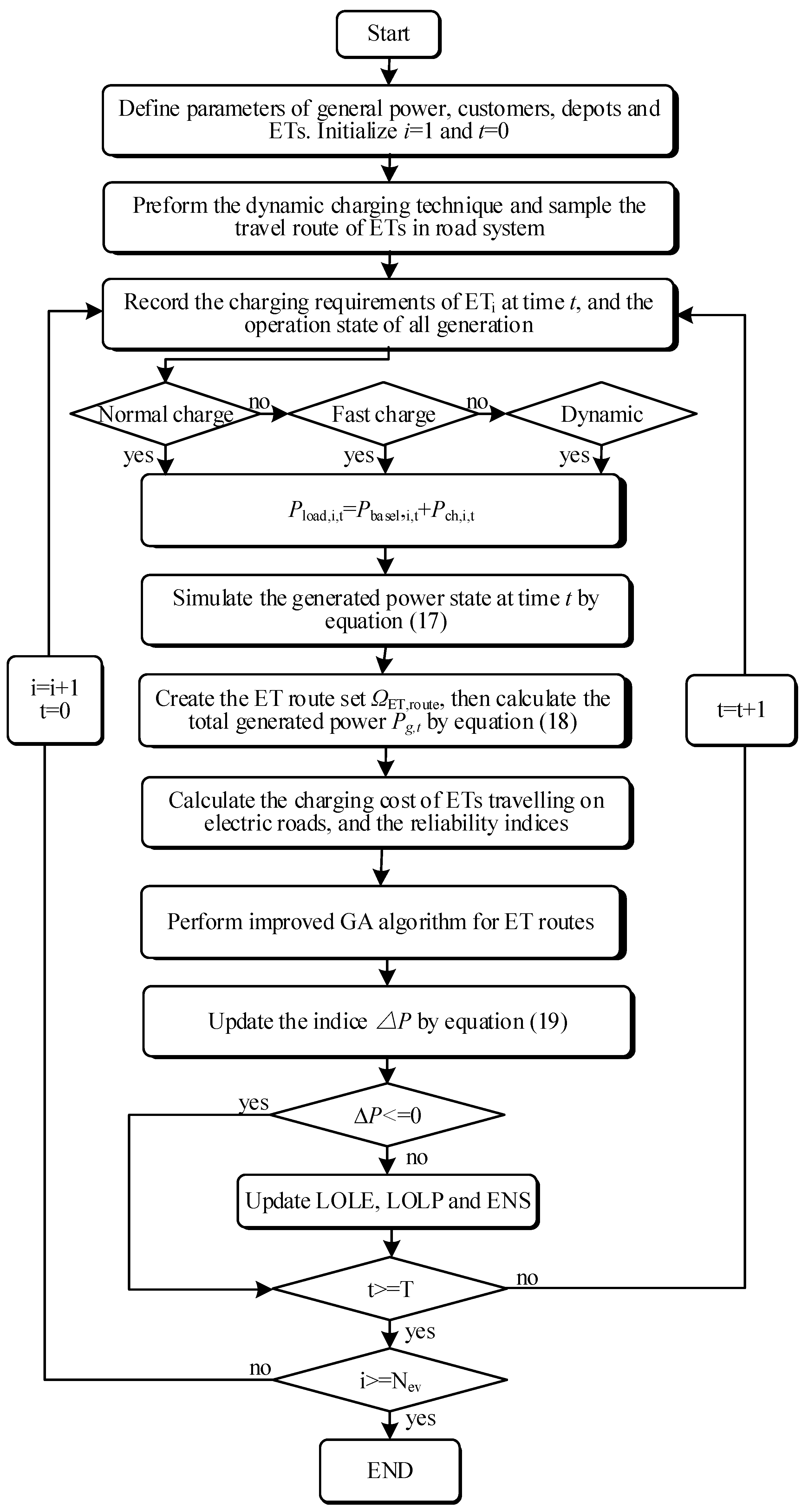
3.2.3. Daily GA-Driven Monte Carlo Simulation-Based Reliability Assessment Method for ETPSS–ER System

In order to compute the reliability indices introduced above, appropriate method needs to be developed for simulating the ETPSS–ER system. Generally, in the ETPSS–ER system, the supplied power comes from the thermal power plants, which is conventionally used to cover the base load. As the most reliable generation technology, its working states mainly have two modes, namely, normal operation and failure, which can be modeled by a two-state Markov chain model, as shown in Figure 3a. It is assumed that the operation and repair times obey exponential distributions. The working states of ’up’ and ’down’ represent the normal and failed operating states, respectively. This implies that the system will stay in one state for a period of time before it changes to the other working state due to failure or reparation. Next, the two states alternate and the durations of the two states include time to failure (TTF) and time to repair (TTR), as shown in Figure 3b.

Accordingly, the system working state and generated system power at time t can be expressed by Equations (18) and (19). Meanwhile, the total generated power is assumed via the inclusion of thermal and wind power generated power, working together for ETPSS–ER power supply.

$$S_{g,i,t}=\left\{\begin{array}{cc}1\hfill & \mathrm{if}\delta <p_{up\to down}\hfill \\ 0\hfill & \mathrm{if}\delta <p_{down\to up}\hfill \end{array}\right.$$

(18)

$$P_{g,t}=\sum _{i=1}^{N_g}{P}_{g,i,t}\times S_{g,i,t}$$

(19)

where $S_{g,i,t}$ and $P_{g,i,t}$ are the state and the power of the $i_{th}$ generators at time t, respectively; 1 means the up state and 0 presents the down state. $p_{up\to down}$ and $p_{up\to down}$ are the transfer probability of up to down state and down to up state. $P_{g,t}$ is the total generated power of thermal generators at time t. $N_g$ is the total number of thermal generators.

In addition, the load power of the $i_{th}$ ET at time t, shown as $P_{ETload,i,t}$, is expressed as Equation (20); the total load model $P_{ETload,t}$ at time t is calculated by Equation (21):

$$P_{ETload,i,t}=\left\{\begin{array}{cc}& P_{slow},ETchargingindepots\hfill \\ \hfill & P_{fast},ETcharginginstations/roads\hfill \\ \hfill & 0,ETnocharging\hfill \end{array}\right.$$

(20)

$$P_{ETload,t}=\sum _{i=1}^{N_{ET}}{P}_{ETload,i,t}$$

(21)

The power shortage $\Delta P_{G,t}$ at time t can be calculated by (22), which is depicted in Figure 4.

$$\Delta P_{G,t}=max\left\{\left(P_{g,t}-P_{basedload,t}-P_{ETload,t}\right),0\right\}$$

(22)

where $P_{baseload,t}$ and $P_{ETload,t}$ are the total base load and ET load demand of the ETPSS–ER system at time t.

For the ETPSS–ER system, the charging load model of ETs and the generated power models have been introduced earlier. Next, a daily travel Monte Carlo simulation method is proposed for ETPSS–ER systems to calculate the reliability indicators. According to their separate delivery tasks, taking the daily travel of ETs as a cycle, the load and supplied power supply can be time-sequentially simulated in minutes. The annual simulation time is usually set to 8760 h. The loop will start from the ET running on the first optimized routes, followed by the next ET until all the routes are simulated and all the customer points have been visited. The proposed daily GA-based Monte Carlo simulation reliability method can be summarized in Figure 5, which has the following steps.

• Initialize parameters of electric road systems, including the number and charging power of trucks, the location and number of customers and depots, and the sampling time;
• Determine the required arrival time, service time, and load requirements for each customer point;
• Generate the delivery routes of ETs to calculate the corresponding charging cost. Then, obtain the optimal ET routes with minimal charging cost by the improved GA algorithm;
• Calculate the load power of ETs traveling on electric roads at time t based on the daily travel and charging routes;
• Update the EVs’ charging and annual load by the load power of trucks charging dynamically on roads;
• Count the total generated power by the annual data and sample the operation state of each generator.
• Determine whether the power supply exceeds the power demand. If this is true, there will be no power shortage; otherwise, there will be a power shortage;
• Calculate the proposed reliability indices, such as LOLE, LOLP, and ENS;
• End the cycle if the time t reaches the total simulation time; otherwise, continue the above steps. Then, update all the reliability indices.

4. Case Study

The case study is conducted using the IEEE Roy Billinton Test System (RBTS) 6-bus system, featuring 6 buses, 11 generators, 9 branches, and 4 loads, with a designated peak power of 185 MW. For the ERS system, ETs with dynamic charging mode are integrated into the system. The paper employs an enhanced Genetic Algorithm (GA) presented in Section 3 to simulate the optimal daily travel routes of ETs, as illustrated in Figure 6. Subsequently, the daily load model is derived through the integration of the ET travel and charging model, facilitating relevant calculations.

4.1. Parameter Settings

In the year 2022, the total number of newly registered electric medium- and heavy-duty trucks was nearly 60,000, which accounted for about 1.2% of truck sales worldwide [29]. There were about 52,000 ETs sold in China, which dominated the production and sales of ETs (86.7%), while UK and Europe sales accounted for 5.2% and 4.7% of the global sales of ETs, respectively [30]. Furthermore, according to the new Global Drive to Zero Emission Technology Inventory (ZETI) database, the number of ET models also continued to expand in 2022, which may be used in the ERS system. Therefore, in this case study, medium-duty ETs are used to build the road traffic model. The related parameters used in the simulation of the ETPSS–ER systems are shown in

Table 3. Parameters of the ETPSS–ER system based on the IEEE RBTS system.

Parameter	Value
Electric trucks number	5
EV charging point ratio (dynamic/static charging point)	$1/10$
EV full-charge driving distance (km)	150
EV full-load capacity (kg)	200
EV static/dynamic charging power in mid-time (kW)	40
EV slow charging power in depot station (kW)	6

.

In this case study, an ET fleet is used for daily delivery within 50 miles of the depot. This ET fleet has five trucks, which can use slow charging in the depot, fast charging at the road charging station, or fast dynamic charging when traveling on the road sections. It is further assumed that all the trucks start from depot and drive back to the depot after delivering all tasks. Hence, the operational framework can be delineated as follows. ETs initiate their journeys at the depot. Subsequently, when the battery capacity becomes insufficient to reach the next delivery location, the ETs proceed to the charging station for battery replenishment. Following this charging interlude, the trucks resume their journeys, completing all assigned delivery tasks. Finally, they return to the depot for parking and subsequent recharging. It is evident that midway charging options, including fast charging and dynamic charging, will benefit the ET fleet operation with a lower number of trucks. In this case, the daily travel plan with minimal cost of ETs driving on the ETPSS–ER system can be achieved by using the proposed GA algorithm method described in Section 3, as shown in Figure 6.

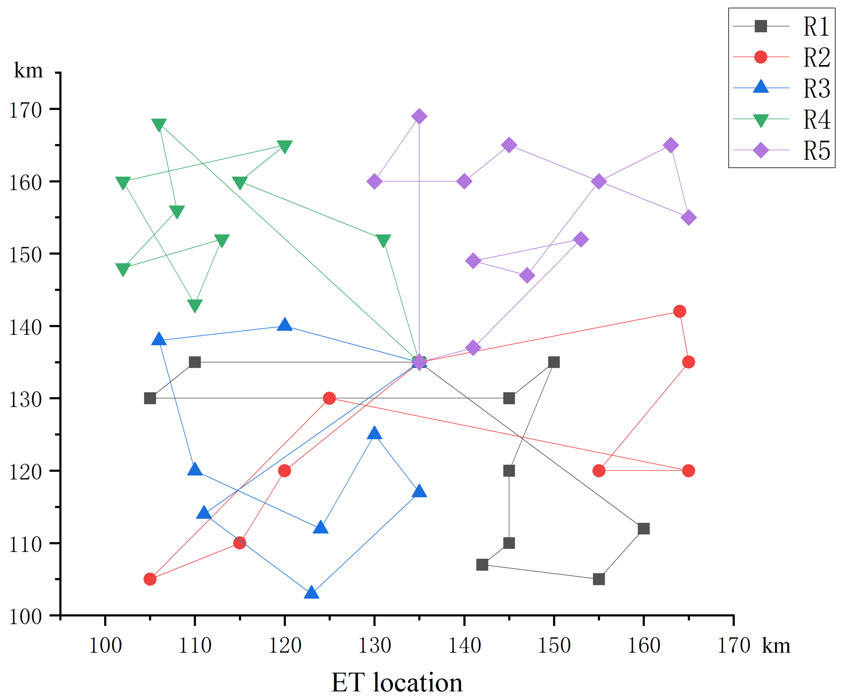
4.2. ET Routing Results

According to the DS–GA algorithm, the optimized ET routes are illustrated in Figure 6. There are five routes for the ETs working for the depot delivery, which are detailed below:

• $0\to 32\to 18\to 33\to 17\to 16\to 8\to 21\to 12\to 45\to 0$;
• $0\to 30\to 10\to 31\to 3\to 20\to 50\to 19\to 23\to 0$;
• $0\to 13\to 36\to 11\to 34\to 9\to 2\to 35\to 42\to 0$;
• $0\to 24\to 14\to 7\to 29\to 4\to 38\to 37\to 41\to 39\to 0$;
• $0\to 22\to 26\to 1\to 40\to 5\to 28\to 27\to 15\to 47\to 6\to 25\to 0$.

Here, number 0 is the depot, and numbers 1 to 40 present the customer locations. Numbers 41–44 and 46–50 are the fast charging locations, while number 45 is the dynamic charging road location. Moreover, it is also assumed that the working time of ETs are 9:00–12:00 and 13:00–17:00.

It is clear that these five ET routes all start from the depot packaged with goods needed to be delivered, then travel to different customer points until the battery capacity cannot support the distance to the next planned point. In the meantime, they travel to the nearest charging point to recharge the power in order to continue the delivery task. For example, the ET on route 1 drives from the depot in the morning, travels through eight customer locations, then goes back to the depot after charging at the electric road section. All the daily charging moments of the five ET routes on the ETPSS–ER system are listed in

Table 4. The daily charging moments of ETs on electric roads.

Route	Charging Moment (Time t)
	Static Charging Midtime	Dynamic Charging Midtime	Static Charging Depot
1	-	14:44	15:23
2	13:37	-	15:34
3	14:13	-	15:01
4	13:41	-	15:39
5	13:55	-	15:55

. It is shown that, on these five routes, only an ET traveling on route 1 uses the dynamic charging mode to recharge the battery. And most of the ETs are charged for the first time while in transit at around 13:00, and return to the depot for the second charging at around 15:00. This has impacts on the peak power demand periods, which may decrease the reliability of the ETPSS–ER systems.

4.3. Reliability Indices

4.3.1. Load Cost–Benefit Model

Based on the optimal ET routes in Figure 6 and the corresponding charging moment in Table 4, the load model of the ETPSS–ER system can be established. It shows that, when considering the mid-charging, five ETs could meet the delivery needs within a given area, taking into account mid-way charging. Moreover, the charging load fluctuation of ETs is presented in Figure 7. It is evident that ETs began to charge at the charging stations in the afternoon at 13:37, until all vehicles were fully charged at around 19:30 in the evening. Therefore, the normal load model of ETs on the ETPSS–ER systems can be established.

Then, the average cost–benefit indices for a specific delivery area supported by the ET fleet are as listed in

Table 5. Charging cost indices for ETPSS–ER power supply.

Indexes	COC (GBP)	MCOC (GBP)	FOC (Times/per ET)	RDC
Value	517.1918	103.4384	2	10%

. This shows that the total daily charging cost for ETs is about GBP 517, while the mean charging cost for an ET is about GBP 100 per day. Meanwhile, each ET has an average of 2 charging times charging while on duty, while the dynamic charging mode in this team accounts 10% of the total charging amount.

4.3.2. Power System Reliability

Table 6. Reliability indices for basic ERS (no trucks) power supply system.

Indexes	LOLE (h)	LOLP	ENS (MWh)
Basic ETPSS–ER	35.0000	0.0040	147.6334
ETPSS–ER with wind power	6.0000	6.8681 × ${10}^{-4}$	21.5492

lists the reliability indices for the ETPSS–ER system with no trucks introduced. These reliability indices mainly show the annual energy shortage situation. It can be clearly seen that the basic annual energy shortage time is around 35 h for about 147 MWh. Generally speaking, to shorten the energy shortage time, introducing additional renewable wind power is an indispensable step for the ETPSS–ER system. Therefore, it is assumed that there are three wind generators introduced here, for which the rated powers are set as 3.5 MW. The corresponding reliablity indices are also illustrated in Table 6. This shows that, when an additional renewable wind power is introduced into the ETPSS–ER system, the power shortage situation has improved significantly. The annual energy shortage hour has decreased from 35 h to 6 h, while the amount of annual energy shortage is reduced from 147 MWh to 21 MWh.

(1) 

Indexes of ET penetration in ETPSS–ER system

In this case, the indexes of the ET number in ETPSS–ER system were determined, as delineated in

Table 7. Reliability indices for basic ETPSS–ER power supply.

Truck Number	LOLE (h)	LOLP	ENS (MWh)
100	35.0000	0.0040	148.2694
300	35.0000	0.0040	149.5412
500	36.0000	0.0041	150.8484
1000	36.3833	0.0042	156.1793
3000	55.9500	0.0064	297.3056
4000	202.7000	0.0232	2647.4440
5000	356.4500	0.0408	10,523.0063

. The results show that the increased number of ETs imposed pressure on the power system. Specifically, the annual energy shortage experienced a notable surge, ranging from 148 to 10,523 MWh as the number of ETs increased from 100 to 5000, accompanied by a substantial increase in load loss hours, escalating from 35 to 356 h. Conversely, within the range of up to 1000 ETs, the energy shortage and load loss indices remained rather constant at 150 MWh and 35 h, respectively. This indicates that the current road power system could accommodate approximately 1000 ETs as the maximal additional load, maintaining stable operation for the ETPSS–ER system.

However, beyond 1000 ETs, particularly when the ET number exceeds 3000, the energy shortage started to intensify. As indicated in Table 7, the introduction of 5000 ETs into the ETPSS–ER system resulted in a critical energy shortage situation. The escalating number of ETs in road systems translates to heightened load demands throughout the day for the power supply system. Consequently, in this context, the incorporation of additional wind power emerges as a viable solution to meet the escalating demands of the ETPSS–ER system.

(2) 

Impact of wind power for ETPSS–ER system

To further alleviate the pressure of ET charging load on the power system, three wind generators were introduced. The rated power of the introduced wind power was 3.5 MW. Then, the reliability indices of the ETPSS–ER system, augmented with renewable wind power, are presented in

Table 8. Reliability indices for ETPSS–ER with integrated wind power.

Truck Number	LOLE (h)	LOLP ($\ast {10}^{-4}$)	ENS (MWh)
100	6.0000	6.8681	21.5492
300	6.0000	6.8681	21.5492
500	6.0000	6.8681	21.5492
1000	6.2333	7.1352	21.5692
3000	13.5333	15.4914	60.7609
4000	110.1667	126.1065	1420.1682
5000	285.4167	326.7133	7895.4413

, encompassing scenarios with 100 to 5000 ETs traveling on the road. A comparative analysis with the basic ETPSS–ER system reveals a pronounced reduction in the energy shortage for the wind-powered ETPSS–ER system, specifically with 1000 ETs, where the power shortage is reduced markedly from 150 to 20 MWh, representing an 85% reduction. Simultaneously, the annual load loss hours also reduced significantly, indicative of a more stable operational environment for the ETPSS–ER system.

(3) 

Impact of BESS for ETPSS–ER system

It is evident that the introduction of additional renewable power can effectively mitigate the pressure on the power system induced by the charging loads of ETs. However, as the number of ETs increases, the energy shortage gap also continues to broaden. Given the uncertainty of wind power, a blanket incorporation of intermittent renewable power into the power system without constraints is evidently impractical. Therefore, the Battery Energy Storage System (BESS), which is capable of managing battery charge and discharge, offers great potential in smoothing the renewable power generation.

The reliability indices for the ETPSS–ER system integrated with wind power and BESS are given in

Table 9. Reliability indices for ETPSS–ER power supply integrated with wind power and BESS.

Truck Number	LOLE (h)	LOLP	ENS (MWh)
3000	13.5333	0.0015	60.7609
4000	109.4000	0.0125	1418.8391
5000	281.2000	0.0322	7863.9448
6000	381.7167	0.0437	17,543.9211
7000	429.1333	0.0491	29,216.4485
8000	454.5500	0.0520	41,285.3816

. Compared with the ETPSS–ER system integrated with wind power, its energy shortage is significantly decreased. Notably, the benefits are apparent when the BESS is integrated into the ETPSS–ER system with wind power.

In summary, for the ETPSS–ER system in the current setting, the introduction of fewer than 1000 ETs usually does not require installation of additional power-generating units such as renewable power. However, as the number of ETs increases, it is necessary to integrate additional renewable wind energy to not only alleviate the power supply pressure of the system, but also to reduce the carbon emissions of the entire road system. In addition, for ETPSS–ER system with high ET load, integrating a BESS system will not only reduce the energy shortage, but will also improve the flexibility of the transportation system.

5. Conclusions

In order to accelerate the transport electrification, the introduction of dynamic charging into the road system will significantly extend the ET driving distance and benefit the roll-out of ETs. However, the escalation of electricity demand due to mass roll-out of ETs also introduces unforeseen reliability challenges to the existing power systems. This study has investigated the reliability of an ETPSS–ER system by considering the introduction of dynamic ET charging and the roll-out of ETs. To achieve this, a comprehensive modeling approach has been proposed, which combines an optimization model for ET routing and a Monte Carlo-based reliability assessment method. The study has investigated the reliability of ETPSS–ER systems considering the roll-out of ETs and the benefits of integrating additional renewable power generation and BESS in alleviating the escalation of power demand due to the increase of ETs and fluctuations of renewable power generation.

The case study results show that, for the specific power system setting, the introduction of 1000 ETs will not cause major impact on the reliability of the existing system. As the number of ETs continues to increase, it will bring huge power demand pressure to the existing power supply system. It is, therefore, valuable to introduce supplementary renewable power into the existing power grid to alleviate the pressure of power demand due to increase in ET roll-out while reducing the carbon emissions. When the number of ETs exceeds 3000, it is necessary to introduce additional renewable power and BESS for more reliable ETPSS–ER system operations.

References

1. Umar, M.; Ji, X.; Kirikkaleli, D.; Alola, A.A. The imperativeness of environmental quality in the United States transportation sector amidst biomass-fossil energy consumption and growth. J. Clean. Prod. 2021, 285, 124863. [Google Scholar] [CrossRef]
2. Ahmadian, A.; Mohammadi-Ivatloo, B.; Elkamel, A. A review on plug-in electric vehicles: Introduction, current status, and load modeling techniques. J. Mod. Power Syst. Clean Energy 2020, 8, 412–425. [Google Scholar] [CrossRef]
3. Nordin, L.; Hellman, F.; Genell, A.; Gustafsson, M. Distribution of Carbon Dioxide Emissions Produced by the Transportation Sector Worldwide in 2022, by Sub Sector; Technical Report; Statista: Hamburg, Germany, 2023. [Google Scholar]
4. Barsali, S.; Ceraolo, M.; Pasini, G.; Poli, D. Managing BEV Charge to Obtain a Positive Impact on a National Power System. Energies 2024, 17, 348. [Google Scholar] [CrossRef]
5. Tromans, P. Electric Car Statistics–Data and Projections; Technical Report; Statista: Hamburg, Germany, 2023. [Google Scholar]
6. Jackman, J. Electric Vehicle Statistics 2023; Technical Report; Statista: Hamburg, Germany, 2023. [Google Scholar]
7. Global EV Outlook 2023; Technical Report; Statista: Hamburg, Germany, 2023.
8. Zacharof, N.; Bitsanis, E.; Broekaert, S.; Fontaras, G. Reducing CO2 Emissions of Hybrid Heavy-Duty Trucks and Buses: Paving the Transition to Low-Carbon Transport. Energies 2024, 17, 286. [Google Scholar] [CrossRef]
9. Martinez-Boggio, S.; Monsalve-Serrano, J.; García, A.; Curto-Risso, P. High Degree of Electrification in Heavy-Duty Vehicles. Energies 2023, 16, 3565. [Google Scholar] [CrossRef]
10. Prussi, M.; Laveneziana, L.; Testa, L.; Chiaramonti, D. Comparing e-Fuels and Electrification for Decarbonization of Heavy-Duty Transports. Energies 2022, 15, 8075. [Google Scholar] [CrossRef]
11. Lee, K.Y.; Bühs, F.; Göhlich, D.; Park, S. Towards Reliable Design and Operation of Electric Road Systems for Heavy-Duty Vehicles Under Realistic Traffic Scenarios. IEEE Trans. Intell. Transp. Syst. 2023, 24, 10963–10976. [Google Scholar] [CrossRef]
12. Bateman, D.; Leal, D.; Reeves, S.; Emre, M.; Stark, L.; Ognissanto, F.; Myers, R.; Lamb, M. Electric Road Systems: A Solution for the Future? Number 2018SP04EN; National Academies: Washington, DC, USA, 2018. [Google Scholar]
13. Schulte, J.; Ny, H. Electric road systems: Strategic stepping stone on the way towards sustainable freight transport? Sustainability 2018, 10, 1148. [Google Scholar] [CrossRef]
14. Wang, B.; Zhao, D.; Dehghanian, P.; Tian, Y.; Hong, T. Aggregated electric vehicle load modeling in large-scale electric power systems. IEEE Trans. Ind. Appl. 2020, 56, 5796–5810. [Google Scholar] [CrossRef]
15. Almutairi, A.; Alyami, S. Load profile modeling of plug-in electric vehicles: Realistic and ready-to-use benchmark test data. IEEE Access 2021, 9, 59637–59648. [Google Scholar] [CrossRef]
16. Shao, S.; Guan, W.; Bi, J. Electric vehicle-routing problem with charging demands and energy consumption. IET Intell. Transp. Syst. 2018, 12, 202–212. [Google Scholar] [CrossRef]
17. Miao, H.; Chen, G.; Li, C.; Dong, Z.Y.; Wong, K.P. Operating expense optimization for EVs in multiple depots and charge stations environment using evolutionary heuristic method. IEEE Trans. Smart Grid 2017, 9, 6599–6611. [Google Scholar] [CrossRef]
18. Lin, J.; Zhou, W.; Wolfson, O. Electric vehicle routing problem. Transp. Res. Procedia 2016, 12, 508–521. [Google Scholar] [CrossRef]
19. Lu, H.; Shao, C.; Hu, B.; Xie, K.; Li, C.; Sun, Y. En-Route Electric Vehicles Charging Navigation Considering the Traffic-Flow-Dependent Energy Consumption. IEEE Trans. Ind. Inform. 2021, 18, 8160–8171. [Google Scholar] [CrossRef]
20. Morlock, F.; Rolle, B.; Bauer, M.; Sawodny, O. Time optimal routing of electric vehicles under consideration of available charging infrastructure and a detailed consumption model. IEEE Trans. Intell. Transp. Syst. 2019, 21, 5123–5135. [Google Scholar] [CrossRef]
21. Shen, H.; Zhou, X.; Ahn, H.; Lamantia, M.; Chen, P.; Wang, J. Personalized Velocity and Energy Prediction for Electric Vehicles with Road Features in Consideration. IEEE Trans. Transp. Electrif. 2023, 9, 3958–3969. [Google Scholar] [CrossRef]
22. Jia, Y.H.; Mei, Y.; Zhang, M. A bilevel ant colony optimization algorithm for capacitated electric vehicle routing problem. IEEE Trans. Cybern. 2021, 52, 10855–10868. [Google Scholar] [CrossRef] [PubMed]
23. Li, C.; Zhu, Y.; Lee, K.Y. Route Optimization of Electric Vehicles Based on Re-insertion Genetic Algorithm. IEEE Trans. Transp. Electrif. 2023, 9, 3753–3768. [Google Scholar] [CrossRef]
24. Engel, H.; Hensley, R.; Knupfer, S.; Sahdev, S. Charging ahead: Electric-vehicle infrastructure demand. McKinsey Cent. Future Mobil. 2018, 8. [Google Scholar]
25. Danese, A.; Torsæter, B.N.; Sumper, A.; Garau, M. Planning of high-power charging stations for electric vehicles: A review. Appl. Sci. 2022, 12, 3214. [Google Scholar] [CrossRef]
26. Al-Saadi, M.; Bhattacharyya, S.; Tichelen, P.V.; Mathes, M.; Käsgen, J.; Van Mierlo, J.; Berecibar, M. Impact on the Power Grid Caused via Ultra-Fast Charging Technologies of the Electric Buses Fleet. Energies 2022, 15, 1424. [Google Scholar] [CrossRef]
27. Shanmugam, Y.; Narayanamoorthi, R.; Vishnuram, P.; Bajaj, M.; Aboras, K.M.; Thakur, P. A systematic review of dynamic wireless charging system for electric transportation. IEEE Access 2022, 10, 133617–133642. [Google Scholar] [CrossRef]
28. Liu, P.; Wang, C.; Hu, J.; Fu, T.; Cheng, N.; Zhang, N.; Shen, X. Joint route selection and charging discharging scheduling of EVs in V2G energy network. IEEE Trans. Veh. Technol. 2020, 69, 10630–10641. [Google Scholar] [CrossRef]
29. The Global Electric Vehicle Market Overview In 2023: Statistics & Forecasts; Technical Report; Statista: Hamburg, Germany, 2023.
30. Trends in Electric Heavy-Duty Vehicles; Technical Report; Statista: Hamburg, Germany, 2023.
Figure 1. Example of an ET’s daily route.
Energies 17 00934 g001
Figure 2. Structure of DS–GA optimization algorithm for the ET routing problem.
Energies 17 00934 g002
Figure 3. Two -state model for the power system.
Energies 17 00934 g003
Figure 4. The daily Monte Carlo power shortage simulation.
Energies 17 00934 g004
Figure 5. Flowchart of the proposed reliability assessment method.
Energies 17 00934 g005
Figure 6. The optimal routes of ETs traveling on electric roads.
Energies 17 00934 g006
Figure 7. The charging load fluctuation of ETs for the ETPSS–ER system.
Energies 17 00934 g007