A Multi-Objective PFC Boost Inductor Optimal Design Algorithm Based on Pareto Front

Abstract

In this study, the inductor optimization design is performed by applying the Pareto optimization technique. As environmental problems emerge, the electric vehicle market is expanding, and accordingly, volume reduction and high efficiency of the onboard charger (OBC) are required. An OBC consists of a PFC stage and a DC/DC stage. The inductor is a major component in a converter and affects the volume and efficiency of the entire converter system. However, reducing the volume of the inductor leads to an increase in loss due to an increase in the change in flux density. Therefore, it is important to derive a suitable design for the target between the two parameters in the trade-off of loss and volume. This paper introduces the optimal design algorithm for boosting inductors of PFC converters in terms of volume and loss. Volume and loss are difficult to compare with each other, making it difficult to set weights. Therefore, Pareto optimization was applied which can be selected according to the needs and purposes of the decision-maker, without weighting as an optimization method. Through a series of procedures of applying Pareto optimization to the inductor design, several optimal inductor designs can be derived. At this time, the optimal designs become a set of designs in which the loss does not decrease without an increase in volume, or the volume does not decrease without an increase in loss. A designer can select a design with an appropriate volume and loss that meets the purpose of the design or preference. Therefore, through the proposed method, the inductor can be flexibly designed according to the target of the application. The proposed algorithm is applied to the interleaved totem-pole bridgeless boost PFC converter, to review its effectiveness. As a result, several inductor designs are derived in the search space, and various optimal designs are visualized through the Pareto Frontier. This facilitates comparative analysis of various inductor designs and helps designers select reasonable inductors. The validity was verified by selecting one of the obtained optimal inductor designs and driving the experiment with the resulting inductor.

1. Introduction

Due to global warming and abnormal climate phenomena, regulations on greenhouse gas emissions are being strengthened, and the supply of electric vehicles is increasing rapidly [1]. The increased research on electric vehicles has also raised the interest in the power conversion devices inside electric vehicles [2]. As a result, high power density and efficiency are required for the Onboard Charger (OBC) installed inside the electric vehicle [3]. The OBC consists of a PFC (Power Factor Correction) stage for improving the power factor, and a DC/DC stage [4].

In order to reduce the volume and achieve high efficiency of OBC, it is essential to reduce volume and loss. In general, one of the elements that occupies a large volume in a converter is a magnetic material [5]. Therefore, in order to reduce the volume of the entire PFC circuit, it is important to reduce the volume of the magnetic material. On the other hand, assuming the same current, selecting a core with a small volume increases the change in flux density, leading to an increase in core loss. As such, volume and loss are in a trade-off relationship that affects oppositely, so the two factors need to be properly considered. In the case of winding loss, the resistance of the winding changes depending on the material or cross-sectional area of the winding, so selecting the winding is also an important design factor to be considered. In consideration of various variables involved in inductor design, it is intended to review which inductor is the best inductor to enable flexible design in terms of volume and loss of inductors.

This paper presents a boost inductor optimal design algorithm to design a multipurpose optimal inductor considering both volume and loss. Optimization methods are discussed to derive the optimal inductor design, and the Pareto optimization technique, which is widely used for optimizing conflicting objective functions, is applied [6]. The Ap and loss of the inductor are set as objective functions, and Pareto optimization is performed in the direction of minimizing them. Unlike the method of pre-weighting and obtaining a single optimal solution, the Pareto optimal derives a set of optimal solutions, so determining the final design depends on the designer’s preference [7]. Therefore, various optimal inductor designs for volume and loss are provided through the proposed algorithm, and a design suitable for the designer’s purpose or target can be selected. As a result, Pareto Frontier shows optimal designs in the search space, compares and analyzes various optimal inductor designs in terms of volume and loss, and helps designers select a reasonable inductor design.

There have been several studies that applied Pareto optimization to the inductor design [8,9]. The Pareto optimization design method for magnetic components of DAB converters is proposed in [8]. In that study, the shape of the core was selected as the PQ core. However, in general, boost converter-based PFC converters mainly use high flux powder cores in consideration of the maximum magnetic density characteristics and air gap characteristics, rather than ferrite PQ cores [10]. In this paper, the core shape was selected for the powder core made of high flux, and the number of parallel cores was added as a design variable in consideration of customization to enable a more detailed design. In addition, the Pareto optimization design method for the magnetic components of the boost converter is proposed in [9]. In that study, the length of each side of the core, the number of strands of the Litz wire, and the number of turns were selected as design variables using a C-shaped core. However, the number of turns and the length of each side are set as design variables, so there are many optimal solutions. Therefore, in this paper, the core size is defined discontinuously in the standard unit using the commonly used core specifications, while the number of cores in parallel is set as design variables to increase flexibility at the height. In addition, the number of turns that do not significantly affect the volume can be decided by setting separate criteria without setting them as design variables, increasing the ease and simplicity.

The proposed algorithm was applied to a converter of arbitrary specification to verify the optimal solution through comparison between the optimized solution and the non-optimized solution. At this time, it was applied to the interleaved totem-pole bridgeless boost PFC converter topology, which is widely used in PFC stages due to its advantages of reducing the number of conductive elements and reducing input current ripple [11]. In addition, the experiment was driven by applying the inductor Pareto optimal design algorithm to the actual PFC converter, and its effectiveness was verified. In the same way, the optimal solution set was derived by applying it to the interleaved totem-pole bridgeless boost PFC converter, and the final design was selected for the desired purpose. The experiment was driven by applying the inductor results and configuring an experimental prototype, and its validity was verified.

2. Pareto Optimization Algorithm

Generally, optimal design has two components: decision and search [12]. The decision means the designer selects the most desirable design solution between the criteria, and search is a procedure to find one or more solutions that desired pay-off between the criteria. Most optimal designs involve trade-offs between multiple evaluation criteria, and the relationship between decision and search can be formed into three categories [13,14].

(1)

Approach to searching the optimal design after deciding the weight (decide→search, priori preference articulation): It is a method for decision makers to find optimal designs after presetting weights for a number of evaluation criteria, and it is the most common method in engineering optimal design problems.

(2)

Approach to repeated decisions and searches (decide ↔ search, progressive preference articulation): It is an approach that repeats decisions and search tasks while continuously changing the weights until the decision maker finds a satisfactory design. It takes a lot of time and effort for repetitive performance.

(3)

After finding a number of optimal design alternatives, the decision maker determines one of them (search → decide, posteriori preference articulation): After obtaining a number of optimal design alternatives first, the decision maker has a way to determine the design alternative that suits their preferences. There is no need to determine the weight in advance, and it has the advantage of simulating the actual decision-making process.

The first method is to find the optimal design after the decision maker determines the weight for each objective function element in advance [15]. Methods for determining weights include WSM (Weighted Sum Model) (Fishburn, 1967 [16]), WPM (Weight Product Model) (Miller and Starr, 1969 [17]), AHP (Analytic Hierarchy Process) (Saaty, 1980 [18]), ELECTRE (Elimination and Choice Translating Reality (Benayoun et al., 1966 [19]), and TOPSIS (Technique for Order Preference by Similarity to Ideal Solution) (Triantaphyllou and Mann, 1989 [20]).

The methods listed above obtain an optimal design that minimizes the objective function. However, most optimal designs involve evaluation items that are difficult to compare with each other (e.g., volume and loss, weight and cost, etc.). In addition, weights are determined by the decision maker’s subjective/qualitative judgment, and even if weights are systematically obtained by a group of experts, they are not an absolute solution to the mutual importance between objective function elements. The second method changes the weights until the optimal solution is satisfactory and requires continuous search work, so it must involve a lot of time and effort. Therefore, in this study, after obtaining multiple optimal solution groups through Pareto optimization, a third method was adopted that allows the decision maker to select the optimal design plan.

A solution in which other objective functions cannot be improved without deterioration of the objective function is called the Pareto solution, and their set is called the Pareto front [21]. It means each solution of the Pareto set contains at least one objective inferior to the other solution in that Pareto set, although both are superior to others in the rest of the solutions in the search space.

2.1. Initialization

Pareto optimization is performed according to the direction to be optimized within limited design conditions. Before performing Pareto optimization, design variables to be arbitrarily changed within a limited range should be set. When designing an inductor, parameters, such as the size of the inductor core, the number of parallel cores, the material, the cross-sectional area of the winding, and the number of turns, can be set as design variables. In this paper, the optimization was performed by fixing the core material and the winding material, and the number of turns is set to the number of turns that have the lowest average loss within the output voltage specification among the possible turns. As a result, the core, the number of parallel cores, and the cross-sectional area of the winding were set as design variables. In this study, for windings, the American wire standard AWG was used. The value to be optimized, the objective function, is volume and loss. Optimization was performed in the direction of reducing the two purposes. As for the constraints, the specifications of PFC, including input and output specifications, maximum flux density, and current density, were considered. The above contents can be summarized as follows.

$$\begin{array}{ll}\mathrm{Find}& \mathrm{c}=\mathrm{Core}\text{’}\mathrm{s} \mathrm{part} \mathrm{number}\\ & \mathrm{p}=\mathrm{The} \mathrm{number} \mathrm{of} \mathrm{cores} \mathrm{in} \mathrm{parallel}\\ & \mathrm{w}=\mathrm{AWG} \mathrm{number}\\ \mathrm{to} \mathrm{minimize}& {\mathrm{A}}_{\mathrm{p}}(\mathrm{c},\mathrm{p},\mathrm{w})={\mathrm{A}}_{\mathrm{p}} \mathrm{of} \mathrm{core}\\ & \mathrm{L}(\mathrm{c},\mathrm{p},\mathrm{w})=\mathrm{Loss}\\ \mathrm{subject} \mathrm{to}& \mathrm{C}=\{{\mathrm{c}}_1, \dots , {\mathrm{c}}_m\}\\ & \mathrm{P}=\{{\mathrm{p}}_1, \dots , {\mathrm{p}}_{\mathrm{n}}\}\\ & \mathrm{W}=\{{\mathrm{w}}_1, \dots , {\mathrm{w}}_{\mathrm{r}}\}\end{array}$$

(1)

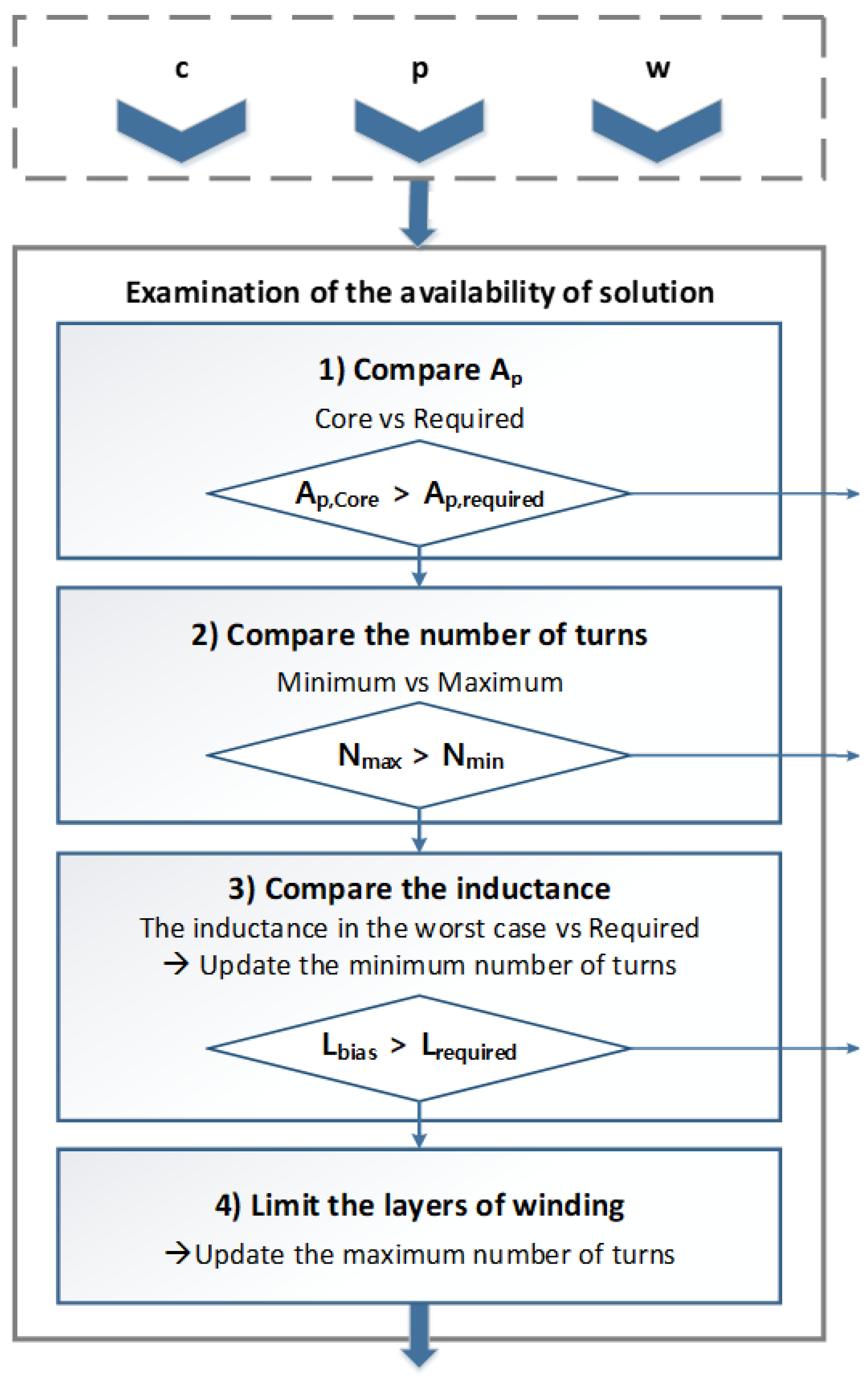
2.2. Examination of the Availability of Solution

When carrying out the design, it is necessary to check that each design variable meets the constraints. However, not all populations meet the constraints. In this case, it cannot be a solution, and if the constraint is not satisfied, a process of exclusion from the solution set is required.

First, the size of the core should be confirmed. Depending on the specifications and constraints of the converter, there is a minimum required A_p [22]. The required inductance is calculated according to design specifications and constraints, such as current ripple and input voltage through (2), and the required A_p is calculated by considering the required inductance and other specifications and constraints through (3) [23]. If the given A_p for each core size and number of parallels is smaller than the required A_p, it is excluded from the immediate solution set without proceeding with the subsequent process.

$$L_{required}=\sqrt{2}{V}_{in,rms}\times (1-\frac{\sqrt{2}{V}_{in,rms}}{V_o})\times \frac{1}{f_s\times I_{ripple}}$$

(2)

$$A_{p,required}=\frac{L\times I_{L,max}}{B_{max}\times pn}\times \frac{I_{L,rms}}{K_u\times J}$$

(3)

Second, the minimum number of turns and the maximum number of turns are compared. For the cross-sectional area (A_e) and winding area (A_w) given for each core size, the minimum number of turns and the maximum number of turns are calculated through (4) and (5). Since the number of turns that can be wound is limited according to the size of the core, the maximum number of turns exists. In the case of A_e, the core cannot be used because it does not satisfy the maximum flux density condition unless it exceeds a certain number of turns. Therefore, depending on the size of the core, there is a range of turns to be satisfied, and if the minimum number of turns is greater than the maximum number of turns, the number of turns available does not exist, so it cannot be a solution.

$$N_{max}=\frac{A_w\times K_u\times J}{I_{in,rms}}$$

(4)

$$N_{min}=\frac{L\times I_{L,max}}{B_{max}\times A_e\times p}$$

(5)

Third, it is necessary to consider the change in inductance according to the change in permeability. Since it is a low-frequency alternating current of tens of Hz, but can be considered a DC bias current in terms of a high-frequency ripple of tens of kHz of an inductor current, it should be designed in consideration of the change in the permeability and the variation in inductance according to DC bias. In particular, high-flux materials must be reviewed because the permeability changes significantly due to the number of turns or currents. The maximum input current is the worst case with the lowest %permeability, so even when the inductance is calculated based on the maximum input current, it should be greater than the minimum inductance required to satisfy the current ripple condition. The required inductance is shown in (2).

If the calculated inductance for the minimum number of turns does not satisfy the required inductance, as can be seen from (6) to (8), the inductance is proportional to the square of the number of turns, so the number of turns must be increased to meet the required inductance conditions. It cannot be a solution if the inductance condition is not satisfied for the maximum number of turns. When the above condition is satisfied, the smallest number of turns among the turns satisfying the condition is updated to the minimum number of turns. The a₁, b₁, and c₁ are unique values of the core material and can be found in the magnetic data sheet. This research fixes a core of a single material but if a core material is to be added as a design variable, it is calculated by changing the constant related to core material characteristics, such as a₁, b₁, etc.

$$H=\frac{4\pi \times N\times I_{L,max}}{l_e}$$

(6)

$$\%\mu =\frac{1}{a_1\times b_1\times H^{C_1}}$$

(7)

$$L=AL\times p\times N^2\times \frac{\%\mu }{100}\times {10}^{-3}$$

(8)

Finally, it limits the number of layers of windings wound around the core. K_u limits the number of turns to a certain level, but if the number of turns is too large, the maximum flux density increases due to self-saturation, increasing the loss of the core, which may increase the heat generation, thereby further limiting the number of layers of winding. This is optional and can be omitted. For the core and winding, the number of turns that can be wound for each layer is calculated, and the maximum number of turns is limited according to the desired number of layers. Comparing the final minimum number of turns with the maximum number of turns, there cannot be a solution if the minimum number of turns is greater than the maximum number of turns.

The procedure for checking whether it can be a solution or not is summarized in Figure 1.

2.3. Calculation of Objective Function

After examining whether or not a solution is possible for all design variables, the objective function is calculated for cases that can become a solution. A_p is determined by the size of the core and the number of parallels. The loss of the inductor consists of core loss and winding loss. The number of turns of winding does not have a significant effect on its volume, so the core loss and winding loss were calculated for all possible turns, and the number of turns with the smallest total loss within the output range was the final turn. The criteria for selecting the number of turns can be changed to suit the purpose desired by the designer. The core loss is affected by a switching frequency, a change in flux density, and the volume of the core. The amount of change in flux density can be obtained through (9) to (11), and the loss can be calculated by integrating every switching cycle, as shown in (12) [24]. The a₂, b₂, c₂, d, e, x, and a₃, b₃, c₃ in the formula can be found in the magnetic data sheet.

$$H_{max}=\frac{4\pi \times N\times I_{L,max}}{l_e}$$

(9)

$$B_{max}={\left(\frac{a_2+b_2\times H_{max}+c_2\times {\left(H_{max}\right)}^2}{1+d\times H_{max}+e\times {\left(H_{max}\right)}^2}\right)}^X$$

(10)

$$△B=B_{max}-B_{min}$$

(11)

$$\sum _T^n{P}_{core}\left(T\right)=a_3\times \sum _T^n{\left(\frac{△B}{2}\right)}^{b_3}\times {f_s}^{C_3}\times V_e\times {10}^{-6}$$

(12)

Winding loss is calculated in consideration of the resistance of the winding material, cross-sectional area, and the number of turns, as shown in (13) and (14). In this paper, the resistance was calculated based on 100 °C in consideration of the evil conditions, and the loss was derived.

$$\mathrm{R}=\frac{\mathsf{\rho }\times (1+\alpha \times \left(T-20\right))\times (N\times MLT)}{W_A}$$

(13)

$$P_{conduction}=R\times {I_{L,rms}}^2$$

(14)

2.4. Derivation of the Pareto Front

Through the series of processes described above, all possible solutions appear in the search space. The Pareto front appears through the solution set created in the search space. The relationship between each optimal solution does not reduce loss without increasing volume, and volume increase is necessarily accompanied by less loss. The following, Figure 2, shows the framework of the algorithm for performing Pareto optimization of the inductor of the PFC converter.

2.5. A Comparative Analysis between Optimal and Non-Optimal Solutions

Previously, the process for Pareto optimal design of the inductor was described. To verify the validity of the proposed algorithm, the aforementioned algorithm was applied to converters of arbitrary specifications. Two Pareto optimal and one non-optimal solution among the resulting solutions were performed in FEM simulations using Ansys Maxwell 3D. Through simulation, the tendency between optimal solutions was identified. In addition, by comparing the optimal solution and the non-optimal solution, it was confirmed that there was a better solution than the non-optimal solution in both volume and loss factors.

One of the topologies applied to the PFC stage is the interleaved totem-pole bridgeless boost PFC converter, and the circuit diagram is shown in Figure 3. The interleaved bridgeless totem-pole boost PFC has a small number of conductive devices, and two inductors are driven through interleaving to cancel out the input current ripple [25]. Therefore, the input current ripple is reduced, thereby reducing the size of the DM (Differential Mode) filter [26]. Due to these advantages, it is one of the topologies widely used in the PFC stage [27]. Analysis between the solutions was performed by applying the above algorithm to the boost inductor of the interleaved totem-pole bridgeless PFC converter.

The specifications of the PFC are shown in

Table 1. The design specifications of the PFC.

Parameter	Value
Input voltage [Vac,rms]	220
Output voltage [V]	400–650
Grid frequency [Hz]	50
Switching frequency [kHz]	50
Power [kW]	3.3

, with an input voltage of 220V_AC, an output voltage of 400–650 V, and a switching frequency of 50 kHz. The current ripple was designed to be 50% considering that the ripple of the inductor current is canceled by the characteristics of the interleaved totem-pole bridgeless boost PFC converter, reducing the input current ripple. The core material was fixed at a high flux 60µ permeability. When comparing copper wire and Litz wire, it is advantageous to use copper wire to secure K_u, and since low-frequency components are major in inductor current, the skin effect can be ignored even if copper wire is used, so it was fixed as copper wire. The design variables are the core’s part number, the number of parallels in the core, and the American wire specification AWG.

The population of design variables is shown in

Table 2. Initial settings of design variables.

Design Variable	Subject
Core’s part number	{CH270060 CH330060 CH343060 CH270060 CH400060 CH467060 CH468060 CH508060}
The number of cores in parallel	{1 2}
AWG	{12 13 14 15 16 17 18 19 20}

. As a constraint, the current ripple was set at 50%, K_u was set to 0.4, and the maximum flux density was set to 1 T in consideration of the margin. At this time, K_u was uniformly applied for ease of design, but if K_u is to be different depending on winding, the constraints according to the design variables can be different and reflected. The layer of winding wound around the core was made possible up to the second layer.

Table 3. Design parameters of arbitrary two Pareto optimal and one non-optimal design plans.

Parameter	Optimized 1	Optimized 2	Non-Optimized
Core’s part number	CH358060	CH467060	CH508060
The number of cores in parallel	2	1	1
AWG	16	14	14
The number of turns	90	77	106
Inductance [µH]	573.84	359.41	359.41
Current density [A/cm2]	614.84	654.67	624.85
Ap [mm4]	49,358	84,973	93,875

shows the design parameters of the two optimal solutions and one non-optimal solution among the solutions obtained as a result of applying the proposed algorithm. The 3D modeling of the three designs for the FEM simulation was shown in Figure 4, and the winding shape was circular, but it was modeled by replacing it with a rectangular winding of the same cross-sectional area in consideration of the simulation time. When the output voltage was 400 V, the flux density and the loss were derived by applying a current for the quarter cycle. Reviewing the flux densities, all of them met the maximum flux density constraint. A_p is directly calculated by the core’s part number and the number of cores in parallel. The tendency among the solutions can be determined by the simulation results of the three designs. The simulation results are shown in Figure 5.

Comparing the non-optimal solution with the optimal solution 2, it can be seen that the optimal solution 2 has a smaller volume and less loss than the non-optimal solution. Therefore, the optimal solution 2 is superior to the non-optimal solution for both elements.

Both optimal solution 1 and optimal solution 2 are optimal solutions, and the simulation results show that solution 1 is smaller for A_p, but solution 2 is less for loss. In terms of volume, solution 1 has a comparative advantage, and in terms of loss, solution 2 has a comparative advantage. Therefore, among the many optimal solutions, designers can choose a design with the desired specifications to suit their volume or loss target.

3. Design Practice

3.1. Application of the Proposed Algorithm

An inductor was designed and selected to drive the actual experiment. The topology is an interleaved bridgeless totem-pole boost PFC converter, the switching frequency is 70 kHz, and other specifications and constraints are the same as the previous settings. The population of design variables is shown in

Table 4. Initial settings of design variables for design practice.

Design Variable	Subject
Core’s part number	{CH270060 CH330060 CH343060 CH270060 CH400060 CH467060}
The number of cores in parallel	{1.0 1.1 1.2 1.3 1.4 1.5 1.6 1.7 1.8 1.9 2.0}
AWG	{12 13 14 15 16 17 18 19 20}

.

3.2. The Result of a Design

All solutions within the range where A_p does not exceed 100,000 mm⁴ were shown, and the optimal solutions were marked with a filled circle. Determining a design may vary depending on the purpose of the designer. The aim of Pareto optimization is to find the optimal balance between conflicting objective functions, not to find a single optimal solution, so the selection must be made with additional criteria. In this paper, a separate selection criterion was set for experimental verification, and the final inductor was taken. The criteria were established that the inductance is within 1.1 times the inductance required to satisfy the current ripple condition, and the loss is within 0.5% of the total system output. There were two optimal designs that met the criteria, and they were displayed in blue in Figure 6. Design parameters for the two solutions are shown in

Table 5. Design parameters of two Pareto optimal design plans.

Parameter	Value
Core’s part number	CH330060	CH400060
The number of cores in parallel	2	1.2
AWG	15	14
The number of turns	71	77
Inductance [µH]	456.95	453.87
Current density [A/cm2]	454.19	359.42
Maximum flux density [T]	0.7489	0.6924
Ap [mm4]	38,966	54,827
Core loss [W]	2.87	3.15
Winding loss [W]	3.99	3.17
Total loss [W]	6.86	6.32

, and an inductor with a smaller volume was selected as the final inductor. An inductor was manufactured based on the parameters, and the manufactured inductor is shown in Figure 7. At this time, since inductance is different for each inductor design plan, controller gain tuning is required when designing the controller according to the inductance of the selected inductor.

For ease of design, the design was carried out by fixing the material as one, but the case where the material was added as a design variable was also reviewed. Optimization was performed by adding materials to design variables, and the additional materials reviewed at this time were high flux 40µ and high flux 125µ. The results are shown in Figure 8. When Pareto optimization was performed by adding other materials, it was confirmed that the selected design was an optimal solution. As mentioned above, the material of the core may be added as a design variable by changing and applying the material-related parameter of the core.

Figure 8 shows the search space reviewed for the three materials. There was no optimal solution with a high flux of 40μ, and there were many optimal solutions with a high flux of 60μ in a region with a small volume. As the volume increased, there were also optimal solutions with a high flux of 125μ. For the PFC specification of this paper, if the volume increases, the design with a high flux of 125μ may have a small loss, but if the volume is small, the material with a high flux of 60μ is considered advantageous.

3.3. Simulation Results

Prior to the experiment, an Ansys Maxwell-based FEM simulation was performed to verify that the selected inductor was properly designed. A current of a quarter cycle of 50 Hz at the output voltage of 400 V was applied.

From Figure 9a, it can be seen that a current of a quarter cycle is flowing into the coil. When the core loss and conduction loss were averaged over the quarter cycle, it had a value similar to the Pareto optimal design value (core loss: 1.639 W, conduction loss: 3.72 W at output voltage 400 V), which confirmed that the design was suitable. In addition, Figure 10 shows that the inductor satisfies the maximum flux density of less than 1 T set as a constraint.

Figure 11 shows the result of loss analysis at the output voltage of 400 V. Switch loss can be derived through formal calculation, but it changes in combination depending on the external environment, temperature, resistance, etc. In addition, since the recovery characteristics, such as recovery time and reverse recovery charge on the data sheet, are only given a value under one condition, there is a limit to the accuracy of calculating through equations. Therefore, in order to derive the loss more accurately, a PLECS simulation was conducted by applying thermal models based on switch data sheets. At this time, the ambient temperature was assumed to be 65℃, and the configuration of the circuit diagram that performed the simulation and the thermal model of the switch are shown in Figure 12, Figure 13 and Figure 14. The predictive efficiency of the entire system based on loss analysis is 98.64% at an output voltage of 400 V, and 98.38% at an output voltage of 650 V.

4. Experimental Results

The experimental prototype is shown in Figure 15. The experimental prototype was composed of three boards. Each is an EMI board, a power board, and an output capacitor board. The EMI board consists of a filter to reduce EMI noise, and the power board has switches and gate drivers. The prototype was constructed by placing the output capacitor board with bulky output capacitors on the power board. Figure 15a shows the top part of the experimental prototype, and Figure 15b shows the bottom part.

Experiments were conducted with AC 220 V input, DC 400, 650 V output, 3.3 kW power, switching frequency 70 kHz, and grid frequency 50 Hz. The experimental specifications are shown in

Table 6. The experimental specifications of the PFC converter.

Parameter	Value
Input voltage [Vac,rms]	220
Output voltage [V]	400, 650
Grid frequency [Hz]	50
Switching frequency [kHz]	70
Power [W]	3300
Low-speed switch (Qsw1–Qsw2)	C3M0030090K (900 V, 63 A, 30 mΩ)
High-speed switch (Qsw3–Qsw6)	C3M0065100K (1000 V, 33 A, 65 mΩ)
Boost inductor (LB)	457 µH (CH330060 2 parallel, AWG 14, 77 turn)
Output capacitor (CPFC)	825 µF (B43541B9337M0 400 V 330 uF 2 series, 5 parallel)

. The prototype was tested using an AC source (MX22.5-3PI, California Instruments, San Diego, CA, USA), power analyzer (WT5000, Yokogawa Test & Measurement Corporation, Tokyo, Japan.), oscilloscope (WaveRunner 8058HD, Teledyne LeCroy, New York, NY, USA), and electronic load (PRODIGIT 34305E, Prodigit Electronics Co., New Taipei City 236, Taiwan).

Figure 16 and Figure 17 show waveforms under 20, 50, 80, and 100% load conditions at output voltages of 400 V and 650 V. When the inductor obtained through the Pareto optimal design algorithm was applied and driven, it was confirmed that the current ripple condition was satisfied and operated stably.

Figure 18 and Figure 19 show the results measured with a power analyzer when the output voltage is 400 V, and the output voltage is 650 V. The results show the input/output voltage, input/output current, input/output power, efficiency, and power factor. The efficiency according to each load is summarized in Figure 20. At the output voltage of 400 V, the full load efficiency was 98.6% and the highest efficiency was 98.81% at 50% load condition. At the output voltage of 650 V, the full load efficiency was 98.14% and the highest efficiency was 98.21% at 80% load condition. When comparing prediction efficiency and actual efficiency, it was confirmed that the design was reasonable with an accuracy of 99% or more. It was confirmed that the power factor was measured higher than 0.99 according to the purpose of the PFC converter. By applying the inductor Pareto optimal design algorithm, the inductor was selected, the experiment was operated, and as a result, it was confirmed that the algorithm could be usefully applied to the design of the inductor.

5. Conclusions

This paper proposed an inductor Pareto optimal design algorithm for designing an optimized inductor in terms of volume and loss. Inductor design variables were set as the core’s part number (the size of the core), the number of parallels, and the cross-sectional area of the winding (AWG), and all design variables were checked to determine whether or not the constraints were satisfied. If all the conditions are met, the objective function is calculated to generate a Pareto front for volume and loss. Applying the Pareto optimization technique, intuitive comparison is possible for all possible inductor designs, which is useful for analyzing them. In addition, it is possible to obtain a solution that meets the needs of decision-makers for Pareto Frontiers. The Pareto optimal solution set was derived by applying the above process to the boost inductor of the interleaved totem-pole bridgeless boost PFC converter. The utility was verified by experimenting with one optimal design plan. It is expected that the results of this study can be easily applied to the design of flexible inductors in terms of volume and loss.