Article

Design, Detection, and Countermeasure of Frequency Spectrum Attack and Its Impact on Long Short-Term Memory Load Forecasting and Microgrid Energy Management †

1
Automotive Engineering Department, Clemson University, Clemson, SC 29634, USA
2
California Independent System Operator (CAISO), Folsom, CA 95630, USA
3
Sandia National Laboratory, Albuquerque, NM 87123, USA
*
Author to whom correspondence should be addressed.
This paper is an extended version of our paper published in Proceedings of the 55th North American Power Symposium (NAPS), Asheville, NC, USA, 15–17 October 2023; pp. 1–6.
Energies 2024, 17(4), 868; https://doi.org/10.3390/en17040868
Submission received: 10 November 2023 / Revised: 22 January 2024 / Accepted: 25 January 2024 / Published: 13 February 2024
(This article belongs to the Special Issue Smart Energy Systems: Learning Methods for Control and Optimization)

Abstract

:
This paper introduces a frequency-domain false data injection attack called Frequency Spectrum Attack (FSA) and explores its effects on load forecasting and the energy management system (EMS) in a microgrid. The FSA analyzes time-series signals in the frequency domain to identify patterns in their frequency spectrum. It learns the distribution of dominant frequencies in a dataset of healthy signals. Subsequently, it manipulates the amplitudes of dominant frequencies within this healthy distribution, ensuring a stealthy attack against statistical analysis of the signal spectrum. We evaluated the performance of FSA on LSTM, a state-of-the-art network for load forecasting. The results show that FSA can triple the Mean Absolute Error (MAE) of predictions compared to the normal case and increase it by 70% compared to noise injection attacks. Furthermore, FSA indirectly enhances battery utilization in the EMS by 45%. We then proposed a detection method that combines statistical analysis and machine-learning-based classification techniques with features. The model effectively distinguishes FSA from healthy and noisy signals, achieving an accuracy of 98.7% and an F1-score of 98.1% on a load dataset, covering healthy, FSA, and noisy load data. Finally, a countermeasure was introduced based on the statistical analysis of the frequency spectrum of healthy signals to mitigate the impact of FSA. This countermeasure successfully reduces the MAE of the attacked model from 0.135 to 0.053, validating its effectiveness in mitigating FSA.

1. Introduction

Microgrids are localized power grids that can operate independently of the main power grid. They are made up of renewable energy sources, storage, and demand-side management technologies, which makes them more resilient, reliable, and flexible than traditional power plants [1]. Within complex and ever-changing energy environments, the significance of an energy management system (EMS) becomes paramount as it actively optimizes the functioning and effectiveness of a microgrid. Load forecasting is an indispensable component of an EMS. It empowers microgrids to plan ahead, enhance energy distribution, manage energy resources, and maintain equilibrium between supply and demand sides. Researchers have dedicated significant effort and attention to implementation of precise load forecasting models. Load prediction utilizes three primary techniques: statistical modeling, machine learning, and deep learning. Deep learning models are superior to other techniques in predictions with high accuracy. Recent advances in computational capabilities of computers have paved the way for deep learning to leverage big data and massive model architectures, resulting in significant improvements in load forecasting accuracy [2]. Due to their embedded memory units that store important temporal inputs, Recurrent Neural Networks (RNNs) often outperform other deep learning architectures, such as Deep Neural Networks (DNNs) and Convolutional Neural Networks (CNNs), when dealing with time-series forecasting tasks [3]. The authors of [4] proposed a new method for short-term load forecasting using a RNN. The proposed method, called MTS-RNN, combines macro- and microinformation using continuous and discrete time series to generate multiple time series (MTS). The MTS are then used to train the RNN model, which can learn sequential information between continuous and discrete series. Nevertheless, RNNs may encounter challenges in grasping long-term dependencies within data, stemming from vanishing and exploding gradient problems. As a result, they may not be well-suited for tasks demanding the representation of extended patterns, such as forecasting electrical load data. Long Short-Term Memory (LSTM) networks are introduced to tackle this issue [5]. While neural networks generally outperform other approaches in various tasks due to their remarkable ability to address highly complex problems in prediction and image classification, their stability under certain circumstances is still a subject of investigation in some studies [6]. Despite their excellent performance in output prediction, recent studies have revealed that deep learning models are more vulnerable than other prediction methods to cyber-security threats [7,8].
Recently, researchers have developed several cyber-attacks on deep learning prediction models and investigated their impacts on the models’ performance. Adversarial attacks [9], data integrity attacks [10], and false data injection attacks [11] are some examples of cyber-attacks on machine learning and deep learning models.
Adversarial attacks are one type of malicious attempt to manipulate inputs to a machine learning model in order to cause it to make incorrect predictions or otherwise degrade the model performance. It is achieved by deliberately adding small perturbations to the input data, which are often imperceptible to humans’ eyes but can cause the model to misclassify the data [12]. Fast Gradient Sign Method (FGSM) [12] and Projected Gradient Descent (PGD) [13] are two significant adversarial attacks. Although adversarial attacks can leave serious degradation impacts in the performance of predictive models, they pose some drawbacks for real-world applications. Crafting adversarial examples can cause a high computational cost for adversaries, especially with respect to complex models or large datasets [14]. In order to launch effective attacks, adversaries must have full knowledge of the targeted model’s structure and trained parameters. However, this level of access is often not feasible in real-world situations, making white-box attacks less practical. Although some research has shown that crafted adversarial examples can be transferred into unknown models, the transferability feature is not fully guaranteed [15]. False data injection attacks (FDIAs) are a significant class of machine learning attacks where malicious actors inject fabricated or manipulated data into the training dataset to compromise the model’s accuracy and performance. Scaling, pulse, ramping, and random attacks are some of the popular FDIAs in the power system load forecasting domain [16,17]. The authors of [18] presented Scaling and Delay Attacks to compromise price information sent to consumers from smart meters and studied their impact on the power system. A scaling factor is introduced to falsify the advertised price on smart meters. The price signal is also corrupted by the false timing information that sends the old price to customers. The authors of [19] developed a detection procedure using sensitivity analysis to track the Scaling and Delay Attack. They also proposed a countermeasure by designing a robust control algorithm and detecting anomalies in the behavior of the system. Signal ramping is another example of a FDIA. The ramp attack is generated by adding positive values from a uniform random function to the true measurements. Studies have shown that ramp attacks are capable of compromising the performance of power systems by reducing frequency balance. Statistical and temporal characterization of the Area Control Error (ACE), generator corrections based on frequency and tie line power flow measurements, is a pivotal approach to detect and mitigate ramp attacks [16].
Despite their simplicity and ease of implementation, the aforementioned FDIAs exhibit limitations in terms of lack of diversity and vulnerability to defense techniques. Scaling attacks commonly center on uniformly perturbing input features using a constant factor, which restricts the diversity of the resulting adversarial examples. As a consequence, these attacks may exhibit reduced efficacy against specific model architectures or data distributions. Various defense strategies, including adversarial training and input preprocessing, can substantially reduce the potency of scaling attacks [20,21]. Consequently, models fortified with these defenses are less susceptible to the impact of such attacks.
FDIAs in the literature are diagnosed through the employment of common statistical and time-series analysis. Since FDIAs are implemented in the time domain, frequency-domain analysis of the corrupted data can easily unveil the malicious activities on data. This paper extends the Frequency Spectrum Attack (FSA), briefly introduced in [22]. It enhances the attack’s stealthiness attribute by transforming time series into a frequency domain, thereby reducing the chances of detection and mitigation by spectrum analysis. The contributions of this paper are below:
1-
The proposed FSA is extended that transforms the load data into the frequency domain and manipulates the amplitudes of dominant frequencies while keeping them in the statistical range of healthy amplitudes to not only cause a huge prediction error but also enhance stealth of the proposed FSA.
2-
FSA is tested on a deep LSTM model to investigate the effectiveness of FSA on the state-of-the-art deep learning model for time-series forecasting. The impact of the attacked LSTM on the EMS’s output of a microgrid is studied as well.
3-
A detection method is proposed, which integrates statistical analysis of the crafted attack and a machine-learning-based classification model to effectively detect the FSA and distinguish it from healthy and noisy signals.
4-
A countermeasure is introduced, based on statistical analysis of the frequency spectrum of healthy signals, to mitigate the impact of FSA on load forecasting.
This approach involves attacking the amplitudes of dominant frequencies of the original data, carefully chosen within a defined range, instead of generating new frequencies like delay or ramp attacks. As a result, the manipulated data remains undetectable through an investigation of the frequency spectrum of compromised data.

2. Frequency Spectrum Attack

2.1. FSA Principles

In this paper, we introduce Frequency Spectrum Attack (FSA), a novel technique performed in the frequency domain. Our approach revolves around investigating the time-dependent behavior of data in the frequency domain through spectral analysis using the Fast Fourier Transform (FFT) technique. By identifying and extracting dominant frequencies with the highest significance, we strategically manipulate their amplitudes to induce substantial, yet undetectable, changes in the original signal’s profile, yet leading to significant signal degradation. Notably, we purposely avoided the manipulation of frequencies, as they are susceptible to detection through spectral analysis tests by grid operators. Our focus on amplitude manipulation ensures that the crafted attack remains stealthy and evades detection, augmenting its potency in compromising the targeted system. Figure 1 elucidates the simple principles of the proposed FSA on a time-series signal.
F 1 and F 2 in Figure 1 are the two dominant frequencies of this specific spectrum. The frequency-attack block consists of three elements. First, the frequency spectrum of the signal is obtained by performing FFT on the original data. In the next step, dominant frequencies, F i s, are extracted and, depending on the adversary’s desire, amplitudes of certain F i s, ( Y F i H s), are manipulated. The superscript H refers to the healthy or original data. Next, corrupted amplitudes ( Y F i F S A s) are achieved by multiplication of Y F i H s and random scaling factors ( α i s), Y F i F S A = α i × Y F i H . The superscript F S A refers to the corrupted data. α i s values are selected within specific ranges derived from statistical analysis of the frequency spectrum of the healthy dataset.
Lastly, the fabricated time-series dataset is reconstructed by performing Inverse Fast Fourier Transformation (IFFT) on the fabricated spectrum. The adversary must ensure that the crafted attack remains undetectable and the constructed signal does not differ significantly from the original signal. Otherwise, the attack will be trivial and easy to detect. Therefore, the adversary must set some criteria on selection of Y F i with the aid of statistical analysis of the healthy dataset. In this case, the knowledge of the historical information and the physical attributes of the signal/data can help in generating undetectable attacks. For instance, the peak-to-peak amplitude of the attacked signal should not be much larger or much smaller than the original one to draw grid operator attention. Similarly, depending on the nature of the signal, some values are not permissible, e.g., a negative value for a current signal. In this paper, we adopted the adversary’s perspective to assess the robustness of the systems. In the next section, we used load time series to further elaborate FSA principles on real-world data and test its performance on a LSTM model as state-of-the-art technology in load forecasting.

2.2. LSTM-Based Load Forecasting

In this paper we applied the proposed FSA method to a load forecasting unit as an EMS component in an islanded microgrid fully presented in our previous work [23]. The objective of this section is to examine the detrimental impact of a crafted FSA on the performance of the power load forecasting unit. For this purpose, we employed LSTM networks, an advanced machine learning technology, as the load forecasting unit to test their resilience against the proposed attack technique.
The load dataset for training, testing, and validation was taken from The New York Independent System Operator [24], from 1 January 2020 to 1 January 2021. A time interval of five minutes was utilized for recording the load data points. The dataset load demand for a year is shown in Figure 2. The dataset is partitioned into three subsets: training, testing, and validation sets. The training set comprises data from 1 January 2020 to 5 October 2020, totaling 80,000 data points. For the validation and test subsets, data from 6 October 2020 to 14 December 2020 (20,000 data points) and 15 December 2020 to 26 December 2020 (1500 data points) are respectively defined.
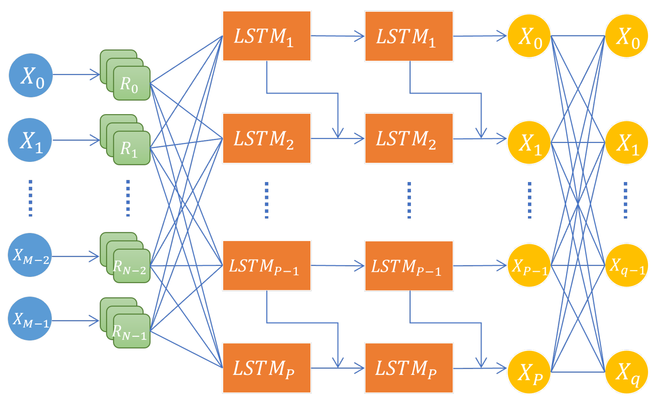
To investigate the strength of the proposed attack, we utilized a deep LSTM network that we presented in [23]. Figure 3 shows the architecture of the deep LSTM model in [23]. The model architecture consists of one input layer, followed by two hidden LSTM layers. Additionally, two Dropout layers are inserted at the end of each LSTM layer to prevent overfitting. Finally, a fully connected feed-forward dense layer is added at the end of the second hidden layer. The performance of the trained LSTM model is evaluated using the validation loss measure.
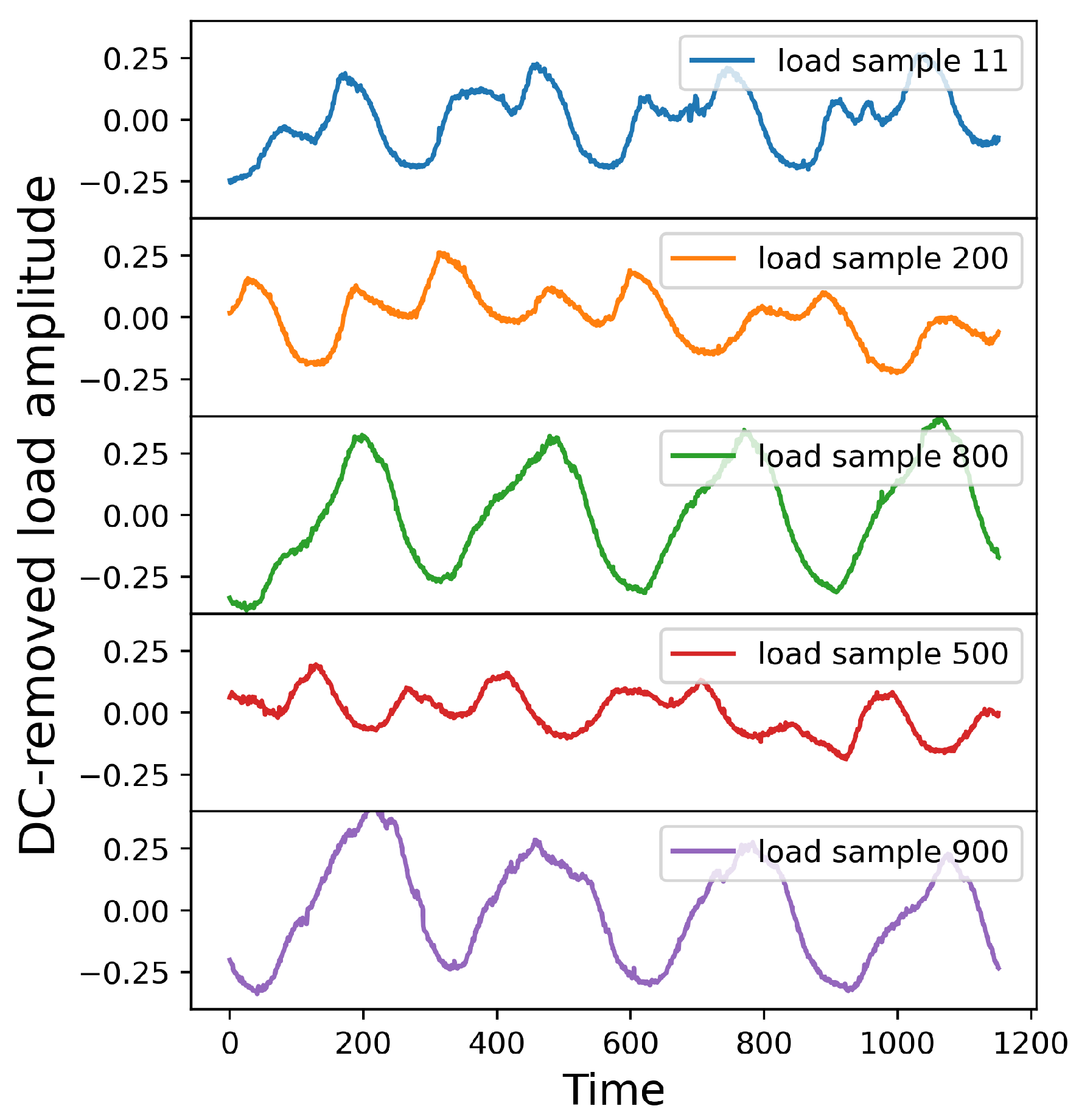
Readers are encouraged to refer to [23] for more information about the model’s architecture and optimal hyperparameters. The input to the LSTM model consists of a four-day load profile, comprising 1152 data points, while the output is a five-hour load prediction in the future, encompassing 60 data points. Figure 4 displays a selection of random DC-removed load profiles extracted from the original load dataset.

3. FSA Implementation

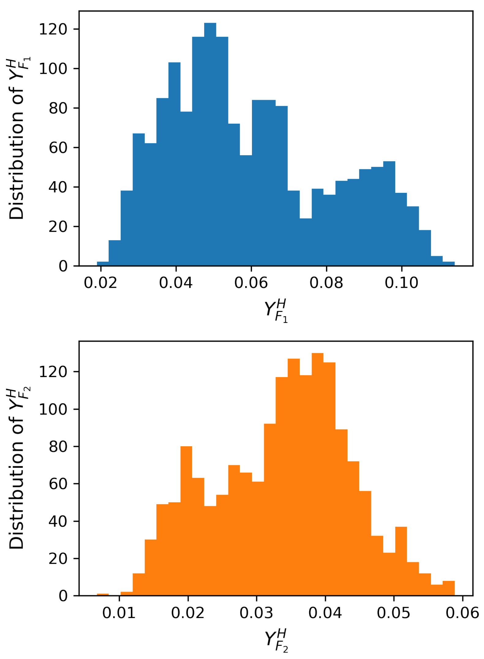
As stated in Section 2.1, our objective is to maintain the attack’s stealthiness while inflicting a substantial impact on the system’s performance. We need to manipulate Y F 1 H and Y F 2 H in a way that makes a stealthy attack. To achieve a stealthy attack, we initiate the process by conducting Exploratory Data Analysis (EDA) on the healthy LSTM input data. During this procedure, we thoroughly investigate the distributions Y F 1 H and Y F 2 H pertaining to the healthy LSTM inputs. The distributions of normalized Y F 1 H and Y F 2 H are displayed in Figure 5. For each LSTM batch, amplitudes are normalized using the maximum amplitude in frequency spectrum of that batch.
Now, if Y F i F S A falls within the healthy range of [ M i n ( Y F i H ) , M a x ( Y F i H ) ] the crafted attack will be considered statistically undetectable. Based on Figure 5, values of [ M i n ( Y F 1 H ) , M a x ( Y F 1 H ) ] and [ M i n ( Y F 2 H ) , M a x ( Y F 2 H ) ] are [0.02, 0.11] and [0.01, 0.06], respectively. Y F i F S A falls within the healthy range of [ M i n ( Y F i H ) , M a x ( Y F i H ) ].
In this section, we evaluate the effectiveness of the proposed FSA on the state-of-the-art time-series forecasting technology, LSTM networks, using a real time-series dataset. Algorithm 1 demonstrates the principles of FSA. First, we obtain [ M i n ( Y F i H ) , M a x ( Y F i H ) ] values where i = 1 , 2 , through an initialization process. Next, a variance range for corrupted data is assumed: [ M i n ( Y F i F S A ) , M a x ( Y F i F S A ) ], such that [ M i n ( Y F i F S A ) , M a x ( Y F i F S A ) ] [ M i n ( Y F i H ) , M a x ( Y F i H ) ] . This constraint guarantees the stealthiness of the FSA in frequency spectrum analysis. M i n ( Y F i F S A ) and M a x ( Y F i F S A ) values are eventually optimized using a Genetic Algorithm (GA) to achieve the FSA range that causes the maximum MAE in LSTM prediction. The scaling factor variation range is selected as α I = [ M a x ( Y F i F S A ) / M i n ( Y F i H ) , M i n ( Y F i F S A ) / M a x ( Y F i H ) ] . Then, the healthy time-series data are transformed by FFT into the frequency domain and the amplitude of the spectrum ( Y F H ) is recorded. In the next step, the healthy amplitude of the dominant frequency, Y F i H , is recorded. Subsequently, the corrupted amplitude of the dominant frequency, Y F i F S A , is generated by multiplying Y F i H with a randomly selected value of α i from the α I range. If Y F i F S A does not fall within the healthy range of Y F i H , a new random α i must be generated and the process continues until the constraint is satisfied. As mentioned earlier, the first two dominant frequencies, F 1 and F 2 , are selected in this study. After GA optimization with all LSTM time-series batches, optimized α I ranges for F 1 and F 2 become [ 0.9 , 9 ] and [ 0.9 , 8 ] , respectively.   
Algorithm 1 FSA Implementation
  1:
for number of F i s do                             ▹ i = 1 , 2 in this study.
  2:
    Initialization:
  3:
    Obtain [ M i n ( Y F i H ) , M a x ( Y F i H ) ]
  4:
    Assume M i n ( Y F i F S A ) and M a x ( Y F i F S A ) such that: [ M i n ( Y F i F S A ) , M a x ( Y F i F S A ) ] [ M i n ( Y F i H ) , M a x ( Y F i H ) ]
  5:
    Define α i range:
α I = [ M a x ( Y F i F S A ) / M i n ( Y F i H ) , M i n ( Y F i F S A ) / M a x ( Y F i H ) ] .
  6:
    Get time-series: X t H .
  7:
     Y F H A m p ( F F T ( X t H ) )
  8:
    Find Y F i H by sorting Y F H components.
  9:
    Randomly select an α i from α I
10:
     Y F i F S A α i Y F i H
11:
    while  Y F i F S A [ M i n ( Y F i H ) , M a x ( Y F i H ) ]  do Go to line 9 again.
12:
    end while
13:
end for
14:
X t F S A I F F T ( Y F F S A )
Some examples of the FSA impact on the LSTM input are shown in Figure 6. As Figure 6 illustrates, some features are noticeable from the proposed attack. Due to the specific optimized α I achieved in this work, the fabricated data can be categorized into three different types. The categories can be different depending on α I ranges: (a) higher amplitude of F 1 for the FSA signal compared to the healthy signal and similar F 2 amplitudes, Y F 1 F S A > Y F 1 H , Y F 2 F S A Y F 2 H , (Figure 6a); (b) the approximately equal amplitudes of F 1 and F 2 in the FSA and healthy signals, Y F 1 F S A Y F 1 H , Y F 2 F S A Y F 2 H , (Figure 6b); (c) 3-higher amplitude of F 2 for the FSA signal compared to the healthy signal and the similar F 1 amplitudes, Y F 2 F S A > Y F 2 H , Y F 1 F S A Y F 1 H , (Figure 6c). Identifying this attack poses a formidable challenge due to its intrinsic nondeterministic nature, setting it apart from other FDIA types like scaling and ramping attacks.

3.1. FSA Results on Load Prediction

The efficacy of FSA is assessed using a trained LSTM model with a test set of 400 input batches. Each batch of healthy input data is subjected to the attack and then fed into the LSTM model. Mean Absolute Error (MAE) per individual recording serves as an evaluative metric for the LSTM model’s performance assessment. For a comprehensive grasp of FSA’s impact, its performance is juxtaposed against scenarios of no attack and noise injection attack. The noise injection attack (SNR = 6–20 dB) is applied to the same LSTM model with the same dataset proposed in [25].
Table 1 presents a comprehensive performance comparison between the proposed FSA and noise injection attack, an alternative FDIA attack. The MAE outcome attributable to the noise injection attack, as documented in [25], is derived from the mean of MAEs resulting from noise attacks at SNR levels of 6–20 dB. The superiority of the proposed FSA manifests in two distinct facets. Firstly, the MAE induced by FSA surpasses the noise attack MAE by approximately 70%. Secondly, while expounded in [25], the noise attack is easy to detect through FFT and frequency spectrum analysis. However, the proposed FSA is stealthy and cannot be detected through FFT or removed by filtering.

3.2. FSA Results on EMS and Microgrid

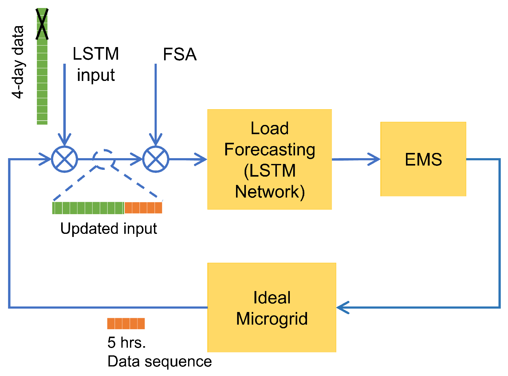
This section delves into the implications of FSA for an Energy Management System (EMS) integrated with an islanded microgrid. The microgrid configuration for this case study is depicted in Figure 7, illustrating its schematic model. The microgrid architecture encompasses two generators, a battery storage unit, and connected loads to a common AC Bus. The PV system is configured to generate a maximum of 600 kW. An MPPT unit regulates the solar panel output to function at the desired voltage, ensuring the attainment of maximum available power. An 8 MWh lithium-ion (Li-Ion) battery and a bi-directional D2D converter are connected to the BESS to manage the battery’s charging/discharging states. Within the inverter block of the battery, a droop controller with virtual inertia is integrated, sourced from [26]. The virtual inertia proves valuable in situations of abrupt voltage or frequency changes. This research operates based on the assumption of an ideal microgrid, wherein controllers can adeptly trace and correct inputs, even when facing sudden variations. As a result, the microgrid’s frequency remains consistently stable, unaffected by the controllers’ input adjustments. Figuratively, the system layout, incorporating the load forecaster, EMS, and islanded microgrid, under the FSA attack, is illustrated in Figure 8.
The comprehensive descriptions of the EMS and the microgrid are meticulously elaborated in [23]. The EMS operates with the purpose of optimizing battery usage within the microgrid system. By determining the optimal points for the Battery Energy Storage Systems (BESS) and Generator Sets (GenSets) for the battery’s inverter and generator controllers, the EMS algorithm seeks to minimize battery utilization effectively. Employing a mixed-integer linear optimization framework with nonlinear constraints, as expounded in [23], the EMS is a sophisticated technique.
The proposed optimization method calculates the 5 h power profiles for the battery ( P B ) and generator ( P G e n ) over the forthcoming 5 h, grounded in predictive power load ( P L ) and solar energy ( P p v ) production. Throughout this study, it is assumed that the solar power profile remains constant across consecutive years. Consequently, if solar data from a single year is at hand, solar power projection becomes unnecessary. The solar resource data originates from the National Renewable Energy Laboratory (NREL) database, as documented in [27].
The majority of cyber-attacks directed at power grids are aimed at the infrastructure itself, with the intention of causing regional shutdowns or blackouts. These attacks inflict substantial damage on the power system, often being swiftly detected and addressed. However, there are situations in which adversaries opt to target the electricity market, manipulating it to favor a specific market player over others. These security challenges are analogous to scenarios encountered in the stock market. Analogous to how stock prices of companies in the same industry often move in tandem due to shared market conditions, the electricity market operates under similar principles. Changes in electricity demand and supply can influence power flow and bidding, potentially favoring particular power generation companies. Though not as overtly destructive as the aforementioned cyber-attacks, these market-oriented attacks result in substantial financial losses within the electricity market, amounting to millions of dollars. A discriminatory electricity market not only skews the market against individual participants but can eventually lead to escalated electricity rates. In this context, Figure 6 illustrates an example of a manipulated load profile that escapes detection via conventional methods or power grid sensors and relays. Such attacks underscore the necessity of innovative approaches to detect, isolate, and manage unconventional attacks like FSA within emerging markets, including the electricity market. This is crucial to ensure fair competition within competitive markets and to uphold the integrity of future markets.
Figure 9 illustrates the impact of FSA on the EMS outputs. We observe harder fluctuations in P G e n under FSA than a no-attack normal condition. More importantly, the average battery utilization ( 1 / N i = 1 N a b s ( P B H o r F S A ) , where N is the LSTM input length) has increased almost 45% under FSA compared to the healthy condition. As the goal of the EMS system was to minimize the battery’s usage, the increment in battery utilization caused by FSA deteriorates the EMS performance.
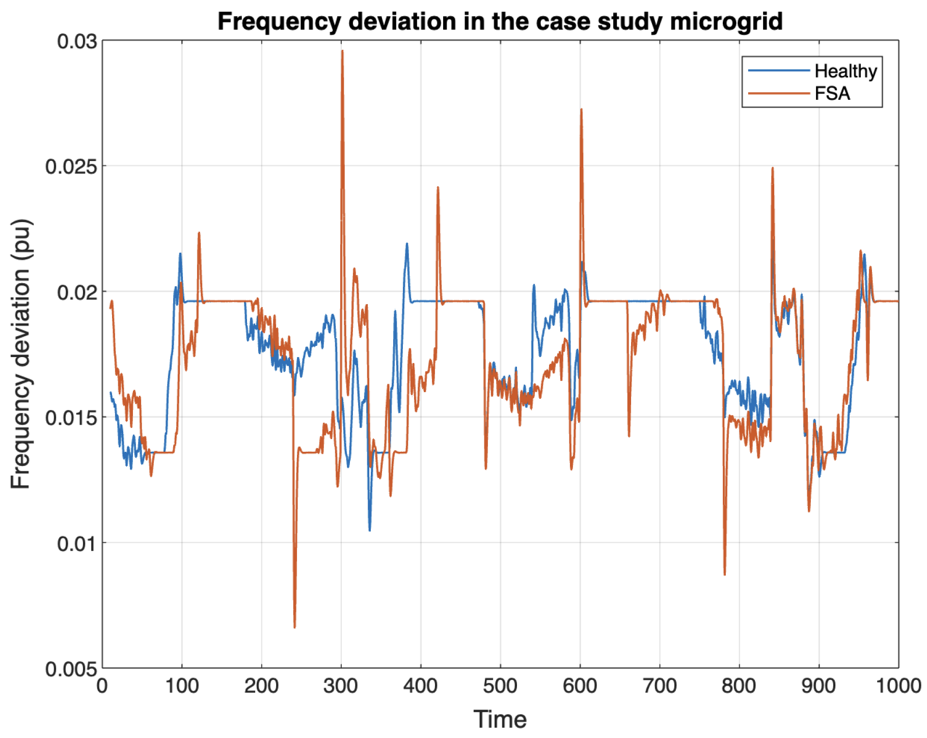
Figure 10 depicts the frequency deviation in the case study model microgrid for a healthy system and a system under FSA attack. It is shown that the attack has been managed such that the generator does not go to the overload mode. Also, the load deviation is smooth and there is no sudden deviation in demand, so the frequency relays wont take any action. The generator control is set to maintain the frequency deviation of less than five percent for normal load deviation. It is shown that frequency deviation under FSA attack still remains less than the standard threshold which is undetectable for frequency sensors.

4. FSA Detection

As we showed, the proposed FSA is a powerful and stealthy attack that can significantly reduce the performance of the load prediction model. Thus, it is of great importance to propose a detection method to accurately detect and isolate FSA attack. In this paper, we examined machine learning classification techniques to propose an efficient classifier to distinguish faulty load data from healthy data. To consider a more realistic and complicated scenario, we assumed that noise attack may also occur. Thus, the model is trained with three types of data including healthy, FSA, and noisy load data. This section is divided into two parts: (a) An explanatory data analysis is conducted on a dataset including healthy, FSA, and noisy load data to extract the useful features for the classification. (b) Based on the selected features in the first part, an efficient classifier is presented by comparing three machine learning classification models to detect and separate the FSA data from healthy and noise-attack data.

4.1. Explanatory Data Analysis of FSA and Statistical Modeling

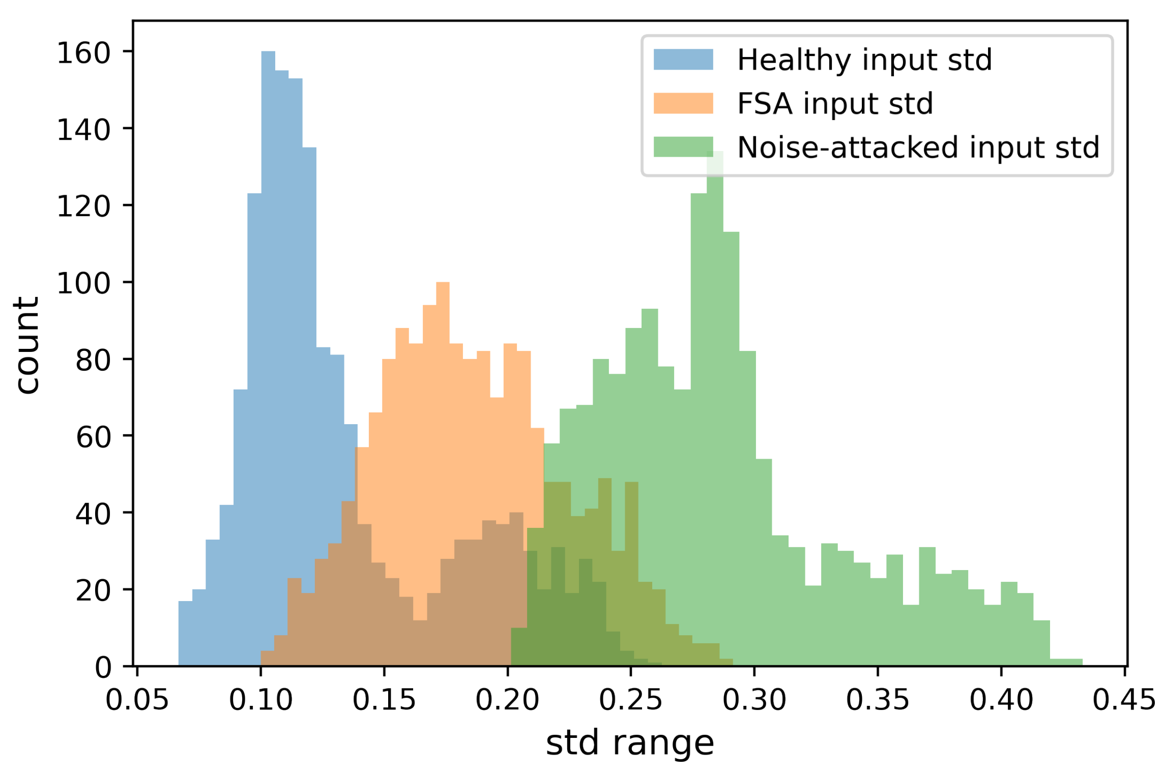
In this section, we investigated the relationships between the FSA, healthy, and noise-attack inputs. Descriptive statistical measures such as mean, standard deviation (STD), interquartile range (IQR), and kurtosis are employed to reveal remarkable information about the dispersion of inputs in these datasets. Later, the significant statistical measures are extracted and selected as features in the classification modeling. The one-year load dataset is divided into 1648 batches of data, each includes 1152 records (4-day load data), as LSTM inputs. Then, FSA and noise attack are applied to these batches. Figure 11 shows the standard deviation distribution of FSA, noise-attack, and healthy LSTM input batches.
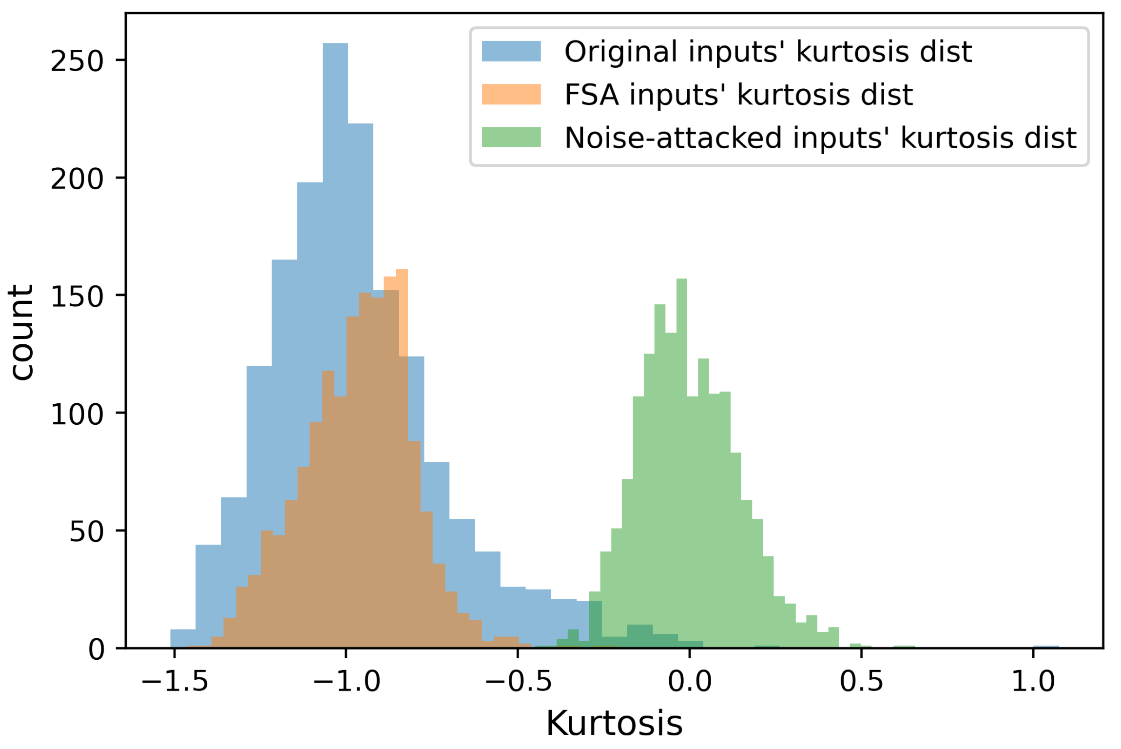
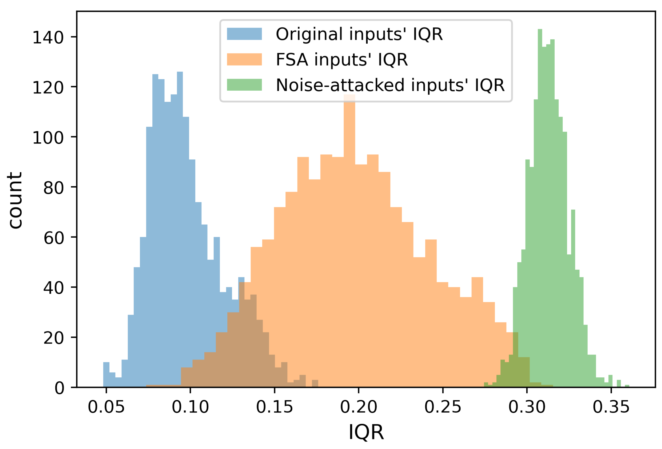
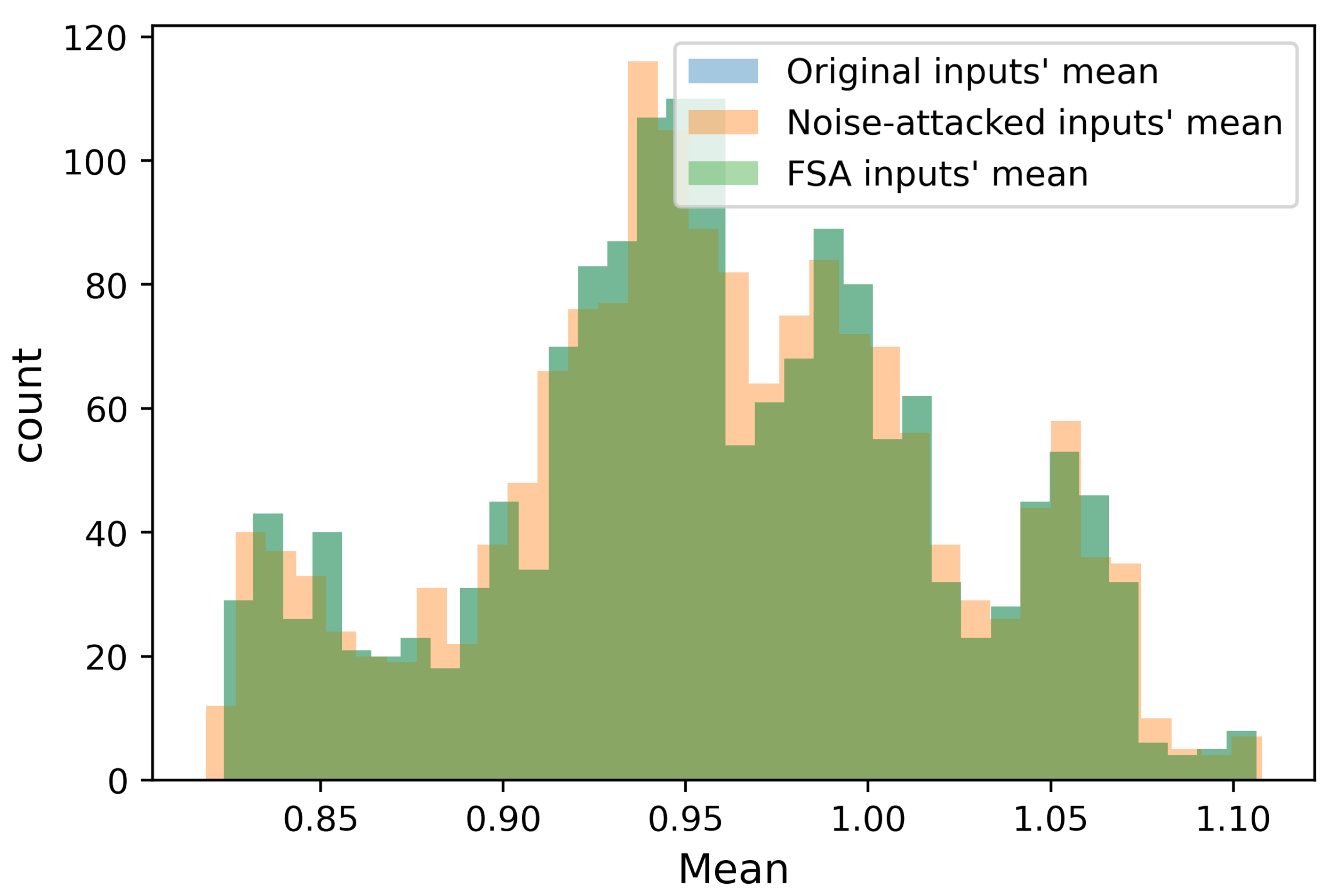
As Figure 11 illustrates, the STD distributions are right-skewed with high variability. Reciprocal Square Root Transformation, ( 1 / X ) , is applied to LSTM inputs’ data to normalize the skewness of the STDs’ distribution and stabilize its variability. Figure 12 depicts the distributions of the STDs after the inputs’ transformation. Figure 13, Figure 14, and Figure 15 show the kurtosis, I Q R / μ , and mean distributions, respectively.
Pearson correlation is a significant tool in data statistical analysis to measure the linear association between two continuous variables. The Pearson correlation coefficient identifies the intensity and direction of the relationship between the variables. This coefficient operates on a scale from −1 to +1, where values closer to −1 or +1 signify a pronounced negative or positive correlation, respectively. A correlation value of 0 implies the absence of a linear relationship.
From Table 2, we observe that STD makes the strongest relationship with the outcome (input label). As expected, some of these measures possess strong linear relationships such as IQR and STD, STD and kurtosis. Next, we applied a multilevel logistic regression model to uncover the relationships between the features and the LSTM input label. Multilevel logistic regression is widely used to analyze binary/nonbinary or categorical dependent variables. The Generalized Linear Model (GLM) from the Python S t a t s m o d e l s library is utilized to investigate the significance of each feature. LSTM input batches are labeled as 0, 1, and 2 representing the healthy, FSA, and noise-attack inputs, respectively. Table 3 presents the coefficient and statistical results of GLM regression, which include the standard error, z-score, p-value, and 95% confidence intervals (CIs) based on hypothesis testing.
Table 3 illustrates the significance of different statistical variables to the output variable (LSTM input type). The results indicate that STD and kurtosis make the most and the least significant relationships with the output variable, respectively.

4.2. ML-Based Attack Detection

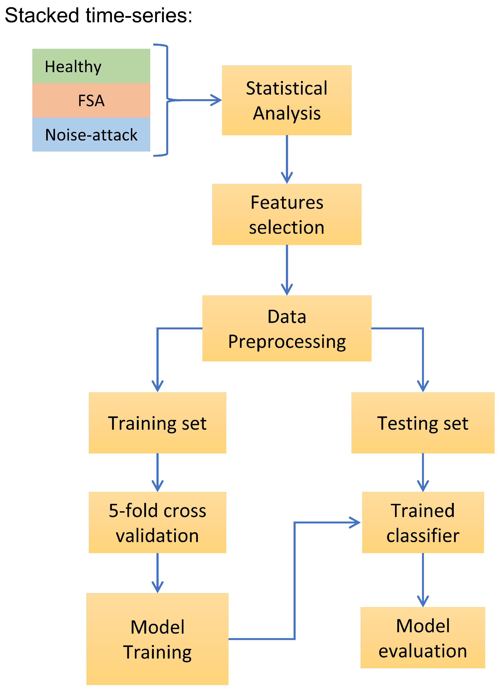
In this section, we propose an accurate machine-learning-based attack detection model with the help of the features extracted in the statistical modeling process. The block diagram of the proposed machine learning-based attack detector is demonstrated in Figure 16. One-year load data is split into 1648 time series each representing 4-day load data (1152 recordings). FSA and noise attack are applied to the time series, and the results are stacked together with healthy load data to generate a dataset for statistical analysis. In the statistical analysis process, four statistical measures, STD, mean, kurtosis, and normalized IQR, are determined for each time series. The time-series statuses are labeled as 0, 1, and 2 representing the healthy, FSA, and noise-attack inputs, respectively, as the dataset’s labels. In the preprocessing part, the dataset is normalized using M i n M a x S c a l e r from the S k l e a r n library, and split into train and test sets with a ratio of 0.2. To improve the performance and generalization ability of the classification model, and to mitigate the chance of over-fitting, fivefold cross-validation is conducted. In summary, the original dataset is randomly divided into five subsets of roughly equal size, with each subset called a fold. The model is trained on four of the folds, referred to as the training set, while the remaining fold is used as the validation set to evaluate the model’s performance. The performance metrics obtained in each iteration are averaged to provide an overall assessment of the model’s performance. Then, the data are fed into a classification model. Finally, the trained classifier is evaluated on an unseen testing set. To find a high-performance model, a number of machine learning classifiers including logistic regression, naive Bayes, and random forest classifiers are tested with five sets of features’ combination. The five sets of features’ combination are: F 1 = [STD, mean], F 2 = [STD, normalized IQR], F 3 = [STD, mean, kurtosis], F 4 = [STD, mean, normalized IQR], and F 5 = [STD, mean, normalized IQR, kurtosis]. Table 4 compares the performance of the proposed classification models using different feature sets. To build a fair comparison between the models and between the different feature sets, hyperparameters of random forest models are tuned for each feature set to achieve the best results. The G r i d S e a r c h C V function from the S k l e a r n library is employed to achieve the best random forest results. Hyperparameters are listed as Number of Trees (NT): [20, 50, 100], Maximum Depth (MD) of each tree: [5, 10, 20], and criterion: [entropy, gini]. In Table 4, the first and the second elements in round brackets are optimal NT and optimal MD, respectively. In this case, the random forest model with NT = 50, MD = 20, and the feature set of F 4 gives the best overall performance with accuracy and F1-score of 98.7% and 98.1%, respectively.

5. FSA Defense

Adversarial detection against machine learning attacks is a hot research area aimed at introducing techniques to identify and mitigate adversarial examples that can deceive or deteriorate the performance of machine learning models. In this section, we introduce a robust statistical-based defense method to mitigate the harmful impact of FSA. First, we utilize the machine-learning-based attack detection introduced in Section 4.2 to distinguish healthy data from FSA data. Healthy data is directly fed into the LSTM forecaster, while the detected FSA input enters a robust statistical-based defense unit to perform sanitation. The defense unit replaces the amplitudes of F 1 and F 2 in the attacked spectrum with randomly selected amplitudes of F 1 and F 2 from the healthy spectrum with a high likelihood of occurrences.
Algorithm 2 presents a step-by-step explanation of the proposed defense method against FSA and noise attack. First, LSTM time-series input data is fed into the defense algorithm. The standard deviation, mean, and normalized IQR of data are obtained through descriptive statistical analysis. In the next step, the extracted features are fed into the optimal classifier, random forest (50, 20), for attack diagnosis. If the classifier detects an FSA, the Fourier Transformer calculates Y F 1 F S A and Y F 2 F S A . Then, the defense algorithm replaces the unknown Y F 1 F S A and Y F 2 F S A with randomly selected known Y F 1 H and Y F 2 H values with a high likelihood of occurrence. Based on Central Limit Theory (CLT), by considering a large sample size, we assume that Y F 1 H and Y F 2 H distributions are approximately normal. In that case, the highest likelihood of occurrence belongs to mean value ( μ ). Y F 1 H and Y F 2 H are drawn randomly from sets of ( μ F 1 H α S E F 1 H , μ F 1 H + α S E F 1 H ) and ( μ F 2 H α S E F 2 H , μ F 2 H + α S E F 2 H ), respectively, where S E denotes the standard error of the original distribution and α is a sampling coefficient. A smaller α denotes a tighter distribution. Finally, if the classifier output is labeled as noise attack, the noise-cancellation model presented in [25] will be applied. Otherwise, the input data remains unchanged and directly moves into the LSTM network. To find the optimal range of sampling, α is tuned and MAEs of load prediction of different α are compared to find the α that makes the minimum MAE. Table 5 elucidates the impact of different α on the proposed defense algorithm performance by monitoring the MAE of the LSTM forecaster. Based on Table 5, Defense 3 is the optimal defense model that minimizes the MAE of load prediction.
Algorithm 2 Defense Algorithm
 1:
Insert time-series input data.
 2:
Carry out descriptive statistical analysis to extract inputs for attack detection classifier.
 3:
Feed extracted features: STD, normalized IQR, mean into classifier.
 4:
Run optimal classifier.    ▹ the output is either healthy, FSA, or noise-attack signals.
 5:
if FSA then
 6:
    Take FFT of LSTM input.
 7:
    Replace Y F 1 F S A and Y F 2 F S A by randomly selected Y F 1 H and Y F 2 H with high likelihood of occurrence.
 8:
    transform data input t-domain by IFFT.
 9:
else if Noise-attack then
10:
    Apply the noise cancellation technique introduced in [25].
11:
else if Healthy then pass.
12:
end if
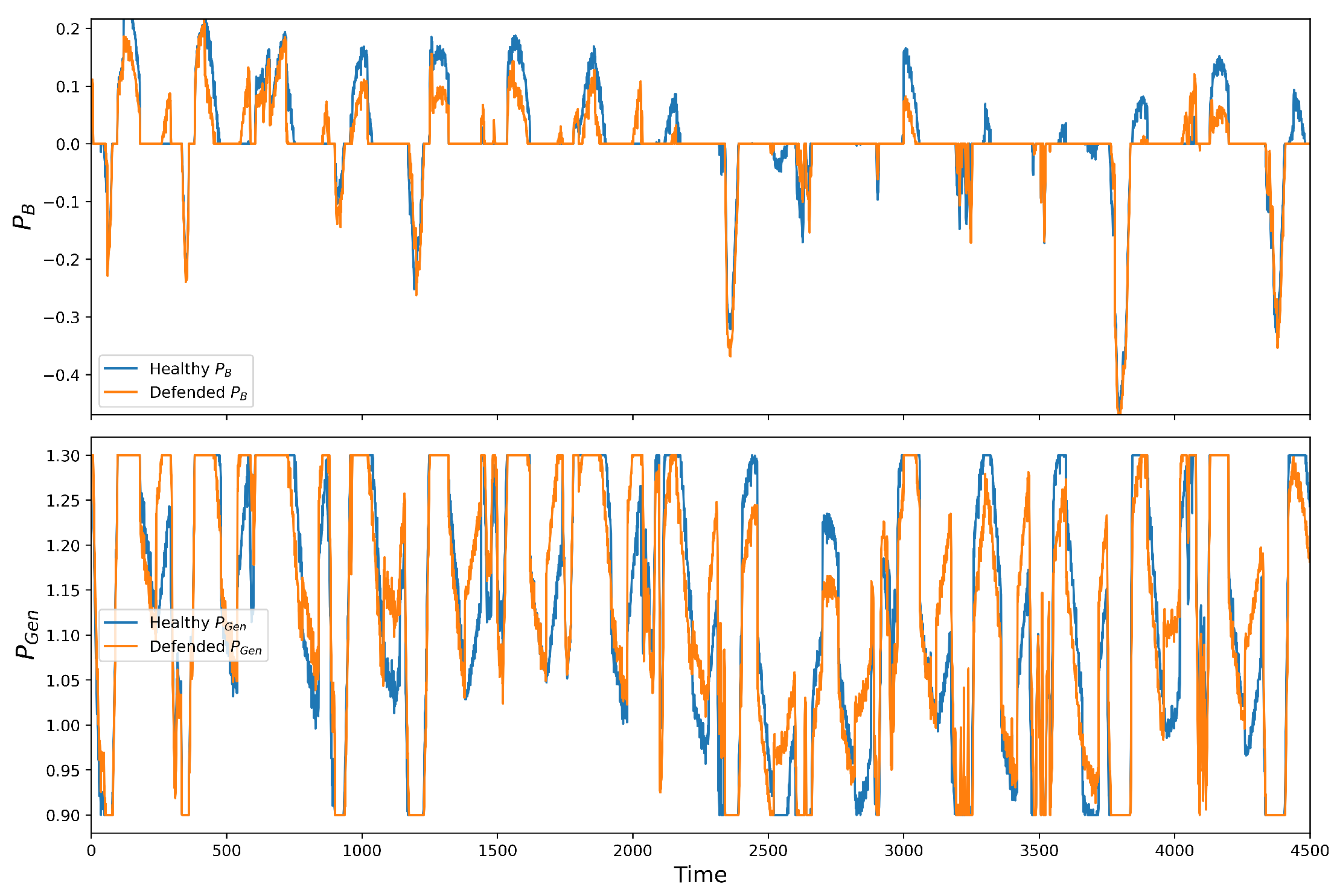
Figure 17 shows the defense strategy impact on the EMS outputs, P B and P G e n . The results represent the role of the proposed defense method in battery utilization enhancement. The P B output of the defended model fluctuates considerably less than the P B under FSA. The battery utilization has reduced by 23% and 60.5% compared to its values in healthy and FSA conditions, respectively. It clearly shows the effectiveness of the proposed defense algorithm as the goal of the EMS optimizer was to minimize the battery’s usage, the defense strategy.

6. Conclusions

In this paper we presented a black-box FSA and investigated its effects on load forecasting and energy management within an islanded microgrid. FSA leveraged Fast Fourier Transform to convert load data into the frequency domain, extracting crucial patterns during the learning phase. By strategically manipulating specific frequencies’ amplitudes within a designated range, FSA maintained its stealthy nature and evaded detection by statistical analysis methods. The evaluation of FSA’s effectiveness on a state-of-the-art deep LSTM network for time-series forecasting revealed a threefold increase in the MAE of load forecasting compared to normal conditions and a 70% increase compared to noise-injection attacks. Moreover, FSA indirectly augmented battery utilization in the EMS by 37.5%. Furthermore, the study demonstrated that FSA successfully eluded frequency monitoring and control units within the microgrid, concealing frequency deviations. To address FSA, a detection method was proposed, integrating statistical analysis and an optimal machine-learning-based classification model with diverse features. This model exhibited high accuracy (98.7%) and an F1-score of 98.1% in distinguishing FSA from healthy and noisy signals on the test set encompassing various load data. Eventually, a countermeasure was introduced, relying on statistical analysis of the frequency spectrum of healthy datasets, effectively reducing the MAE of the model under FSA from 0.135 to 0.053. This demonstrated the countermeasure’s efficacy in mitigating the adverse impact of FSA on load forecasting.

Author Contributions

Conceptualization, A.N. and P.P.; Methodology, A.N.; Software, A.N.; Validation, A.N., P.P. and R.B.; Formal Analysis, A.N.; Investigation, A.N.; Resources, P.P.; Data Curation, A.N. and R.B.; Writing—Original Draft Preparation, A.N.; Writing—Review and Editing, A.N., P.P. and D.S.; Visualization, A.N.; Supervision, P.P.; Project Administration, P.P.; Funding Acquisition, P.P. All authors have read and agreed to the published version of the manuscript.

Funding

Sandia National Laboratories, a multimission laboratory managed and operated by National Technology and Engineering Solutions of Sandia, LLC, a wholly owned subsidiary of Honeywell International, Inc., the U.S. Department of Energy under contract DE-NA0003525.

Data Availability Statement

The dataset is publicly available online on http://mis.nyiso.com/public/.

Acknowledgments

The authors gratefully acknowledge financial support from the U.S. Department of Energy’s Energy Storage Program, managed by Imre Gyuk.

Conflicts of Interest

The authors declare that the research was conducted in the absence of any commercial or financial relationships that could be construed as a potential conflict of interest.

Abbreviations

The following abbreviations are used in this manuscript:
FSAFrequency Spectrum Attack
FFTFast Fourier Transformation
IFFTInverse Fast Fourier Transformation
LSTMLong Short-Term Memory
MAEMean Absolute Error
EMSEnergy management system
RNNRecurrent Neural Network
DNNDeep Neural Network
CNNConvolutional Neural Network
MTSMultiple time series
FGSMFast Gradient Sign Method
PGDProjected Gradient Descent
FDIAFalse data injection attack
ACEArea Control Error
EDAExploratory Data Analysis
GAGenetic Algorithm
SNRSignal-to-noise ratio
NRELNational Renewable Energy Laboratory
STDStandard deviation
IQRInterquartile range
GLMGeneralized Linear Model
CIconfidence interval
NTNumber of Trees
MDMaximum Depth of each tree
CLTCentral Limit Theory

References

  1. Hirsch, A.; Parag, Y.; Guerrero, J. Microgrids: A review of technologies, key drivers, and outstanding issues. Renew. Sustain. Energy Rev. 2018, 90, 402–411. [Google Scholar] [CrossRef]
  2. Wang, P.; Liu, B.; Hong, T. Electric load forecasting with recency effect: A big data approach. Int. J. Forecast. 2016, 32, 585–597. [Google Scholar] [CrossRef]
  3. Dong, X.; Qian, L.; Huang, L. Short-term load forecasting in smart grid: A combined CNN and K-means clustering approach. In Proceedings of the 2017 IEEE International Conference on Big Data and Smart Computing (BigComp), Jeju Island, South Korea, 13–16 February 2017; pp. 119–125. [Google Scholar] [CrossRef]
  4. Zhang, B.; Wu, J.L.; Chang, P.C. A multiple time series-based recurrent neural network for short-term load forecasting. Soft Comput. 2018, 22, 4099–4112. [Google Scholar] [CrossRef]
  5. Van Houdt, G.; Mosquera, C.; Nápoles, G. A review on the long short-term memory model. Artif. Intell. Rev. 2020, 53, 5929–5955. [Google Scholar] [CrossRef]
  6. Li, B.; Liao, M.; Xu, C.; Chen, H.; Li, W. Stability and Hopf Bifurcation of a Class of Six-Neuron Fractional BAM Neural Networks with Multiple Delays. Fractal Fract. 2023, 7, 142. [Google Scholar] [CrossRef]
  7. Chen, Y.; Tan, Y.; Zhang, B. Exploiting Vulnerabilities of Load Forecasting through Adversarial Attacks. In Proceedings of the Tenth ACM International Conference on Future Energy Systems, New York, NY, USA, 25–28 June 2019; pp. 1–11. [Google Scholar] [CrossRef]
  8. Akhtar, N.; Mian, A. Threat of adversarial attacks on deep learning in computer vision: A survey. IEEE Access 2018, 6, 14410–14430. [Google Scholar] [CrossRef]
  9. Huang, S.; Papernot, N.; Goodfellow, I.; Duan, Y.; Abbeel, P. Adversarial attacks on neural network policies. arXiv 2017, arXiv:1702.02284. [Google Scholar]
  10. An, D.; Yang, Q.; Liu, W.; Zhang, Y. Defending against data integrity attacks in smart grid: A deep reinforcement learning-based approach. IEEE Access 2019, 7, 110835–110845. [Google Scholar] [CrossRef]
  11. Lin, J.; Yu, W.; Yang, X. On false data injection attack against multistep electricity price in electricity market in smart grid. In Proceedings of the 2013 IEEE Global Communications Conference (GLOBECOM), Atlanta, GA, USA, 9–13 December 2013; pp. 760–765. [Google Scholar]
  12. Goodfellow, I.J.; Shlens, J.; Szegedy, C. Explaining and harnessing adversarial examples. arXiv 2014, arXiv:1412.6572. [Google Scholar]
  13. Madry, A.; Makelov, A.; Schmidt, L.; Tsipras, D.; Vladu, A. Towards deep learning models resistant to adversarial attacks. arXiv 2017, arXiv:1706.06083. [Google Scholar]
  14. Zhang, J.; Li, C. Adversarial examples: Opportunities and challenges. IEEE Trans. Neural Netw. Learn. Syst. 2019, 31, 2578–2593. [Google Scholar] [CrossRef]
  15. Nowroozi, E.; Mekdad, Y.; Berenjestanaki, M.H.; Conti, M.; El Fergougui, A. Demystifying the transferability of adversarial attacks in computer networks. IEEE Trans. Netw. Serv. Manag. 2022, 19, 3387–3400. [Google Scholar] [CrossRef]
  16. Sridhar, S.; Govindarasu, M. Model-based attack detection and mitigation for automatic generation control. IEEE Trans. Smart Grid 2014, 5, 580–591. [Google Scholar] [CrossRef]
  17. Moradzadeh, A.; Mohammadpourfard, M.; Konstantinou, C.; Genc, I.; Kim, T.; Mohammadi-Ivatloo, B. Electric load forecasting under False Data Injection Attacks using deep learning. Energy Rep. 2022, 8, 9933–9945. [Google Scholar] [CrossRef]
  18. Tan, R.; Badrinath Krishna, V.; Yau, D.K.; Kalbarczyk, Z. Impact of integrity attacks on real-time pricing in smart grids. In Proceedings of the 2013 ACM SIGSAC Conference on COMPUTER & Communications Security, Berlin, Germany, 4–8 November 2013; pp. 439–450. [Google Scholar]
  19. Giraldo, J.; Cárdenas, A.; Quijano, N. Integrity Attacks on Real-Time Pricing in Smart Grids: Impact and Countermeasures. IEEE Trans. Smart Grid 2017, 8, 2249–2257. [Google Scholar] [CrossRef]
  20. Ntalampiras, S. Detection of Integrity Attacks in Cyber-Physical Critical Infrastructures Using Ensemble Modeling. IEEE Trans. Ind. Inform. 2015, 11, 104–111. [Google Scholar] [CrossRef]
  21. Yan, W.; Mestha, L.K.; Abbaszadeh, M. Attack detection for securing cyber physical systems. IEEE Internet Things J. 2019, 6, 8471–8481. [Google Scholar] [CrossRef]
  22. Nazeri, A.; Biroon, R.A.; Pisu, P. Black-Box Stealthy Frequency Spectrum Attack on LSTM-based Power Load Forecasting in an Energy Management System with Islanded Microgrid. In Proceedings of the 2023 North American Power Symposium (NAPS), Asheville, NC, USA, 15–17 October 2023; pp. 1–6. [Google Scholar] [CrossRef]
  23. Nazeri, A.; Biroon, R.A.; Westman, J.K.; Pisu, P.; Hadidi, R. Machine Learning-assisted Energy Management System for an Islanded Microgrid and Investigation of Data Integrity Attack on Power Generation. In Proceedings of the 2022 North American Power Symposium (NAPS), Salt Lake City, UT, USA, 9–11 October 2022; pp. 1–6. [Google Scholar] [CrossRef]
  24. In Proceedings of the The New York Independent System Operator—NYISO. Available online: http://mis.nyiso.com/public/ (accessed on 1 January 2020).
  25. Nazeri, A.; Pisu, P. LSTM-based Load Forecasting Robustness Against Noise Injection Attack in Microgrid. arXiv 2023, arXiv:2304.13104. Available online: http://arxiv.org/abs/2304.13104 (accessed on 25 April 2023).
  26. Dinkhah, S.; Cuellar, J.S.; Khanbaghi, M. Optimal Power and Frequency Control of Microgrid Cluster with Mixed Loads. IEEE Open Access J. Power Energy 2022, 9, 143–150. [Google Scholar] [CrossRef]
  27. In Proceedings of the National Renewable Energy Laboratory. Available online: https://www.nrel.gov/gis/solar.html (accessed on 1 January 2020).
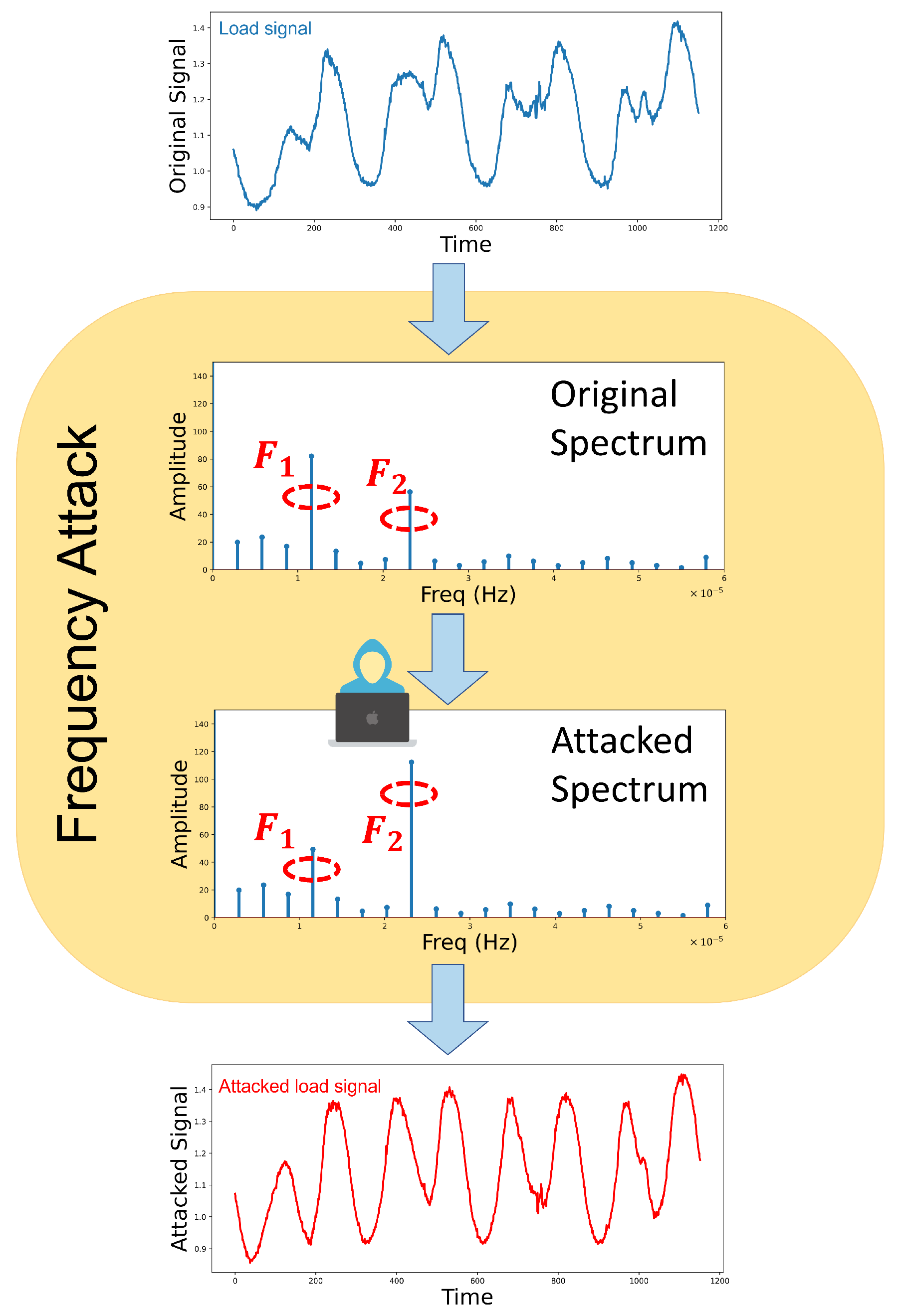
Figure 1. The schematic of the proposed FSA operation.
Energies 17 00868 g001
Figure 2. The one-year cleaned load profile [23].
Energies 17 00868 g002
Figure 3. The architecture of the deep LSTM model [23].
Energies 17 00868 g003
Figure 4. Snapshot of a selection of random DC-removed load data samples.
Energies 17 00868 g004
Figure 5. Distribution of dominant frequencies’ amplitudes ( Y F i H s) of healthy dataset.
Energies 17 00868 g005
Figure 6. Examples of the results of FSA on LSTM time-series inputs.
Energies 17 00868 g006
Figure 7. Case study islanded microgrid.
Energies 17 00868 g007
Figure 8. The schematic of a microgrid EMS under Frequency Spectrum Attack.
Energies 17 00868 g008
Figure 9. FSA results on P B and P G e n .
Energies 17 00868 g009
Figure 10. Frequency deviations in case study microgrid.
Energies 17 00868 g010
Figure 11. STD distribution of the healthy, FSA, and noise-attack inputs.
Energies 17 00868 g011
Figure 12. STD distribution of the healthy, FSA, and noise-attack transformed inputs.
Energies 17 00868 g012
Figure 13. Kurtosis.
Energies 17 00868 g013
Figure 14. Interquartile range.
Energies 17 00868 g014
Figure 15. Mean.
Figure 15. Mean.
Energies 17 00868 g015
Figure 16. The block diagram of the machine-learning-based attack detection.
Energies 17 00868 g016
Figure 17. Defence results on P B and P G e n .
Energies 17 00868 g017
Table 1. The Frequency Spectrum Attack performance.
ScenarioMean Absolute Error (MAE) Per
Recording [MWatt]
No attack0.046
Noise injection attack [25]0.079
Our proposed FSA0.135
Table 2. The correlation matrix for statistical measures.
STDKurtosisIQRMeanInput Label
STD10.8250.9310.0490.961
Kurtosis0.82510.756−0.0090.795
IQR0.9310.7561−0.0980.945
Mean0.049−0.009−0.0981−0.001
Input label0.9610.7950.945−0.0011
Table 3. Generalized Linear Model regression results.
CoefficientStandard
Error
z P > | z | [0.025–0.975]
@%95 CI
Intercept−0.66200.048−13.7500.000(−0.756, −0.568)
STD6.52430.13946.9020.000(6.252, 6.797)
Kurtosis0.05920.0105.8470.000(0.039, 0.079)
IQR3.50190.09038.9330.000(3.326, 3.678)
Mean0.12900.0492.6560.008(0.034, 0.224)
Table 4. Machine learning classification models’ performance with different feature sets.
ML ModelFeatures SetF1-ScoreAcc
Logistic RegressionF10.950.9676
Logistic RegressionF20.970.98
Logistic RegressionF30.9540.968
Logistic RegressionF40.970.98
Logistic RegressionF50.9720.981
Naive BayesF10.960.973
Naive BayesF20.9730.982
Naive BayesF30.9610.974
Naive BayesF40.9730.982
Naive BayesF50.9750.983
Random Forest (50, 10)F10.9570.97
Random Forest (50, 5)F20.9730.982
Random Forest (50, 20)F30.9630.975
Random Forest (50, 20)F40.9810.987
Random Forest (50, 10)F50.9780.985
Table 5. Effect of sampling coefficient α on MAEPR.
Defense ModelSampling RangeMAEPR
Defense 1 μ ± S E 0.058
Defense 2 μ ± 0.5 S E 0.054
Defense 3 μ ± 0.25 S E 0.053
Defense 4 μ ± 0.15 S E 0.054
Disclaimer/Publisher’s Note: The statements, opinions and data contained in all publications are solely those of the individual author(s) and contributor(s) and not of MDPI and/or the editor(s). MDPI and/or the editor(s) disclaim responsibility for any injury to people or property resulting from any ideas, methods, instructions or products referred to in the content.