Short-Term Forecast of Photovoltaic Solar Energy Production Using LSTM

Abstract

In recent times, renewable energy sources have gained considerable vitality due to their inexhaustible resources and the detrimental effects of fossil fuels, such as the impact of greenhouse gases on the planet. This article aims to be a supportive tool for the development of research in the field of artificial intelligence (AI), as it presents a solution for predicting photovoltaic energy production. The basis of the AI models is provided from two data sets, one for generated electrical power and another for meteorological data, related to the year 2017, which are freely available on the Energias de Portugal (EDP) Open Project website. The implemented AI models rely on long short-term memory (LSTM) neural networks, providing a forecast value for electrical energy with a 60-min horizon based on meteorological variables. The performance of the models is evaluated using the performance indicators MAE, RMSE, and R², for which favorable results were obtained, with particular emphasis on forecasts for the spring and summer seasons.

1. Introduction

With the development of modern society, there has also been a growing exploration and excessive use of fossil energy (coal, gas, and oil), which is responsible for 75% of greenhouse gas emissions. This has put significant pressure on the planet’s climate due to the effects such emissions generate. In addition to these environmental concerns, geopolitical constraints and dependence on other countries have led to renewable energy sources such as hydroelectric, wind, solar, and geothermal energy becoming more relevant in the proportion of individual energy sources used for electricity generation. Thus, in the short term, there is an intention to have an electricity sector based on renewable energy sources, as they do not produce any type of pollution. This offers fundamental aid in reducing emissions to mitigate global warming. Fossil fuels are considered only a transitional step toward this future vision [1].

One of the major challenges today in making the electrical grid dependent on renewable energy lies in the nature of climatic conditions, such as solar radiation, temperature, environment, and wind speed, which directly influence energy production and are difficult to predict. Photovoltaic energy forecasts are employed to ensure the efficient management of the electrical grid, as well as in energy trading operations, in which producers face penalties for deviations between production forecasts and actual output. Forecasting models for photovoltaic solar energy have traditionally been based on the mathematical modeling of physical components until recent advancements in artificial intelligence have enabled predictions through machine learning algorithms using representative records of historical photovoltaic production data [1].

The presence of artificial intelligence is continually growing, and as a result, there are currently numerous research efforts related to solar energy production using this technology. The authors [2], in their study, forecast energy production at photovoltaic solar plants using long short-term memory (LSTM) models and a back-propagation neural network (BPNN). The forecast was made for a 15-min horizon based on information from the previous hour. The research was conducted with real data from a station in Brazil, and it highlights the effectiveness of the LSTM model with four layers, showcasing low seasonal error rates. The authors concluded that LSTM outperforms BPNN by providing more accurate predictions. They emphasized the practical applicability of LSTM in hybrid energy production systems or microgrids, demonstrating the importance of accuracy in forecasting to avoid financial penalties and optimize the profitability of photovoltaic plants. An author [3] studied the performance of using LSTM, bidirectional LSTM (BiLSTM), and a temporal convolutional network (TCN) for predicting the power of a photovoltaic solar power plant at the Technical Support Centre of Rey Juan Carlos University (Madrid, Spain). They used one year of data from the plant sampled every 15 min to predict the corresponding power, efficiency, and voltage with a horizon of 15 min and 24 h. The TCN network showed better forecasting results compared to the other networks, and the BiLSTM showed better results compared to the LSTM in terms of the mean squared error (MSE) indicator. Authors [4] explored the use of LSTM models to predict solar energy generation. Their research focused on comparing independent LSTM models with hybrid models that combine LSTM with other techniques. The study used time series data to train and evaluate the models, applying metrics such as the root mean squared error (RMSE) to measure the accuracy of the predictions. The results indicate that pure LSTM models outperform other conventional machine learning approaches, especially in forecasting solar irradiance and photovoltaic power. However, hybrid models, despite requiring more training time, generally perform better in more complex scenarios. The article [5] discusses short-term (24-h) photovoltaic energy prediction using a combined regression-based method. This method aims to enhance energy prediction accuracy by combining five random forest (RF) prediction models with different parameters. A support vector machine (SVM) was used in conjunction with k-means clustering to further improve the method’s accuracy. To select the best hyperparameters for the five models, linear regression and support vector regression were used, with the least absolute shrinkage and selection operator (LASSO) and Ridge serving as regularization methods. The method outperformed the best RF model by 20% and achieved an improvement of 2% over the reference model, recurrent neural networks (RNNs), demonstrating that ensemble prediction strategies yield better accuracy than individual prediction models. Authors [6] used data from the Department of Systems Engineering and Automation at the University of the Basque Country. They implemented artificial neural networks (ANNs) to predict temperature and solar radiation. They also executed a hybrid control technique, JAYA-SMC, to predict, control, and search for the maximum power of photovoltaic panels and adjust the duty cycle of a single-ended primary-inductor converter (SEPIC) that powers a direct-current (DC) motor. This article indicates that having hidden layers provides a competitive advantage in predictive analysis. The central focus of the work [7] was the use of a learning-based, dual-stream neural network that combines convolutional neural networks (CNNs) and LSTM networks to predict solar energy production. CNN was employed to learn spatial patterns, while LSTM was incorporated for the extraction of temporal features. The spatial and temporal feature vectors were merged, followed by a self-attention mechanism (DSCLANet) to select optimal features for further processing through fully connected networks (DENSE). The network’s effectiveness was evaluated using real data, demonstrating a significant reduction in errors compared to recent methods. The importance of accurate solar energy generation prediction was emphasized, helping avoid penalties in energy markets. The authors acknowledged the complexity of DSCLANet, employing two architectures (LSTM and CNN) and expressing the intention to develop a unified architecture in the future. They also expressed an interest in exploring emerging technologies, such as probabilistic forecasting, incremental learning, and reinforcement learning, to further enhance solar energy predictions.

The current article aims to explore the applications of deep learning in the context of solar energy systems, specifically to predict photovoltaic energy production based on real data collected in Faro, Portugal, during the year 2017. For prediction, a recurrent neural network was used to extract temporal information, and fully connected layers were employed to make energy forecasts. Our main contributions are as follows:

• The prediction of photovoltaic solar energy over a 60-min horizon (with data collected every 1 min) using only meteorological variables;
• The construction of a model with a simple architecture utilizing LSTM layers and fully connected layers (DENSE);
• The evaluation of the prediction accuracy of the model for various values of model hyperparameters and different input variables;
• The training, validation, and testing of the model for various seasons of the year and a comparison of the results using performance indicators, namely mean absolute errors (MAEs), RMSE, and the coefficient of determination ($R^2$);
• A comparison of the model’s accuracy with other simple architectures (BiLSTM, gated recurrent units (GRUs), and an RNN) and hybrid architectures (CNN + LSTM).

Another important aspect is the focus on the Portuguese context, providing specific insights into photovoltaic energy production in Portugal, which is particularly relevant in optimizing local energy production.

This article is organized as follows. Section 2 introduces the essential concepts of artificial intelligence required for the prediction model and various performance indicators used in regression models. It also provides the details of the LSTM network used in this study. Section 3 provides a description of the data sets that served as the foundation for the implementation of the models. Section 4 addresses data processing to establish the basis for the prediction models, as well as identifying the optimal features for these models. All the steps involved in modeling the prediction models are also presented. Section 5 presents the results of the work, while Section 6 presents a comparison study between several forecasting models. Finally, in Section 7, the main conclusions are drawn.

2. State of the Art

Artificial intelligence (AI) is a field of computer science that focuses on creating computer systems capable of performing tasks that typically require human intelligence, such as visual perception and speech recognition. AI can be divided into various subfields, one of which utilizes large neural networks to learn and represent complex information.

Machine learning is a subfield of AI that specifically concentrates on developing algorithms with the ability to learn from provided data and make decisions based on observed patterns in that data. Instead of programming specific rules for a task, the system is trained with data, enabling it to learn how to perform the task automatically. Typically, these algorithms require structured input data that are pre-labeled, along with expected outputs, to train the system. Once trained, the algorithm can predict output variables (results) based on the provided inputs [8].

The algorithms that can be created in machine learning depend on the type of solution desired. Therefore, there are three main types of algorithms that can be employed: supervised learning, unsupervised learning, and reinforcement learning. Among these, supervised learning is the most commonly used in both machine learning and deep learning contexts [8].

Deep learning involves mathematical models implemented using an ANN with the aim of imitating the functioning of the human brain. Typically, it consists of an input layer, multiple hidden layers, and an output layer. In Figure 1a, an example of such a network is presented using fully connected layers (DENSE). The hidden layers in the network can consist of various neurons, as shown in Figure 1b. Neurons between each layer are connected via links. Each link has a weight and can receive a value from the neuron in the previous layer. Through activation functions such as the sigmoid function, hyperbolic tangent function, or rectified linear unit (ReLU), the value that goes to the next node is determined. This process is repeated until the final layer (output layer), where the final value is calculated. If the number of hidden layers in the ANN is at least two, then the network is called a deep neural network (DNN).

The more hidden layers there are in a DNN, the more complex the network becomes, potentially leading to an increase in its efficiency. In a structure of this kind, there must always be a compromise between the number of hidden layers and the requirement for what needs to be predicted. Increasing the complexity of the network beyond what is necessary causes the network to start exhibiting poor efficiency for non-existent data, making the choice of the number of hidden layers extremely important [9].

There are various types of network architectures used in deep learning, each designed for specific tasks. It is possible to follow the architecture of feedforward neural networks (FNPs), where information flows in a single direction, from input to output without cycles or feedback [10]. CNNs are designed to extract spatial features in data such as images, where they are highly effective in computer vision tasks [11]. RNNs allow for the handling of temporal data, featuring connections that form cycles and enabling information to be retained over time [12]. LSTM networks, an extension of RNNs, are designed to overcome the vanishing gradient problem and are particularly useful for capturing long-term dependencies in temporal sequences [13].

2.1. LSTM Network

Among the models used in deep learning, one that stands out is the LSTM artificial neural network. This network addresses the gradient problem of traditional RNN, which struggled to update weights at the beginning of sequences. With LSTM networks, it became possible to propagate information over long sequences using forget and update gates. In this way, at each moment in the sequence, data influence the decision to forget (approaching zero) or increment (adding to hidden layers) information.

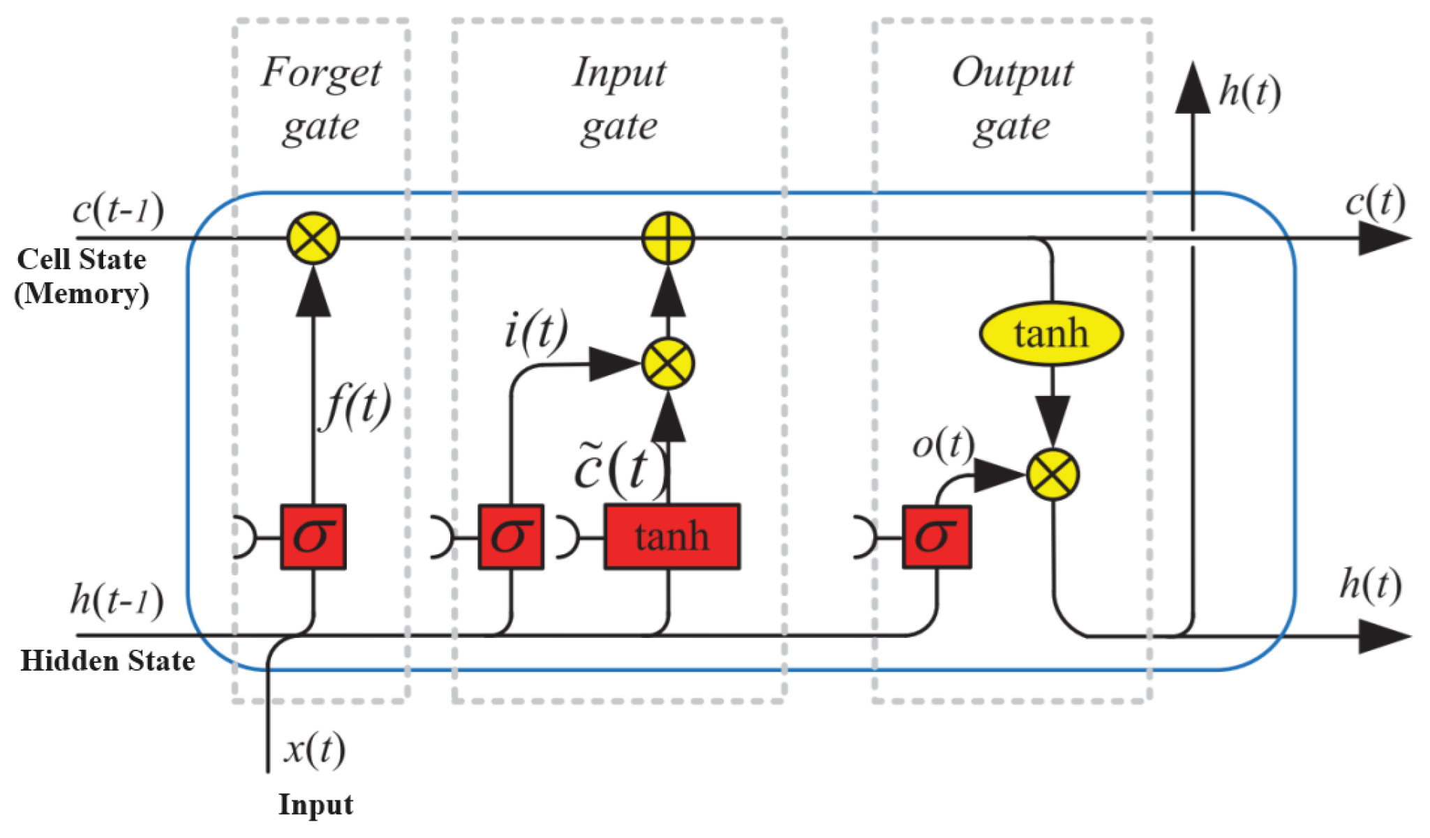
The fundamental idea behind the functioning of LSTM memory cells is the updating of the cell state, visualized as the horizontal line at the top of Figure 2, which is the central component responsible for the flow of information over time [14].

The LSTM cell has the ability to add or remove information from the cell state through structures known as gates. These gates are located in different neural layers of each cell and are composed of functions called sigmoid functions and a multiplication operation. The sigmoid function maps its inputs to output values in the range between 0 and 1, acting as a filter that blocks or lets through a certain component. A zero value at the sigmoid’s output means that the corresponding component will be blocked, while a value of one means that the component will be fully used.

Each LSTM cell has three gates to control and protect the cell state [14].

2.2. How an LSTM Cell Works

The first step in the LSTM process involves deciding which information from the past will be eliminated from the cell-state line (Figure 2). This decision is made through a layer called the forget gate, connected to a sigmoid layer with an input vector of $[h_{t-1},x_t]$ and an output between 0 and 1 for each value in the cell-state line from the previous state, $C_{t-1}$. A value of 1 means that the entire value will be retained, while a value of 0 means that the value will be completely discarded. Thus, the output of the forget gate function, denoted as $f_t$, is given in Equation (1) [14].

$$f_t=\sigma (W_f·[h_{t-1},x_t]+b_f)$$

(1)

The output of this layer updates the cell state by multiplying the $f_t$ function with the values resulting from the cell state line of the previous state.

The next step is to decide what new information will be stored in the cell state line, which is done in the input layer. The input layer consists of two layers: a sigmoid layer and a hyperbolic tangent (tanh) layer. The sigmoid layer decides which input values should be updated through the function $i_t$ shown in Equation (2). The hyperbolic tangent layer creates a vector of new values that can be added to the cell state line ${\tilde{C}}_t$, as shown in Equation (3) [14].

$$i_t=\sigma (W_i·[h_{t-1},x_t]+b_i)$$

(2)

$${\tilde{C}}_t=tanh(W_c·[h_{t-1},x_t]+b_c)$$

(3)

The functions $i_t$ and ${\tilde{C}}_t$ are combined through the multiplication operation that defines the scalar value to be introduced into the vector of probable values. This output is then applied to a summation with the output value from the previous layer, the forget gate, to update the cell-state row, which now becomes $C_t$ (Equation (4)).

$$C_t=f_t\ast C_{t-1}+i_t\ast {\tilde{C}}_t$$

(4)

Finally, there is an output layer consisting of a sigmoid layer (Equation (5)), which filters the input values, and a copy of the cell state $C_t$, which is applied to a hyperbolic tangent function. Both results are then applied to a multiplication operation that will determine the result of the hidden state row that moves on to the next cell (Equation (6)) [14].

$$o_t=\sigma (W_o·[h_{t-1},x_t]+b_o)$$

(5)

$$h_t=o_t·tanh\left(C_t\right)$$

(6)

2.3. Performance Indicators

There are several metrics that can be employed to evaluate the performance of a linear regression model. Some common indicators include MSE, RMSE, MAE, R², and MAPE [16].

MSE allows for the calculation of the average of the squared errors between predicted values (${\widehat{y}}_i$) and actual values ($y_i$) across a certain number of observations (n):

$$MSE=\frac{1}{n}\sum _{i=1}^n{(y_i-{\widehat{y}}_i)}^2$$

(7)

The RMSE (Equation (8)) is the square root of the MSE, and it provides a more intuitively interpretable measure of error since it is measured in the same units as the response variables. In both MSE and RMSE, a lower value indicates better model performance.

$$RMSE=\sqrt{MSE}$$

(8)

The MAE (Equation (9)) calculates the average of the absolute values of errors, and it is less sensitive to distant values (outliers) when compared to the MSE [15].

$$MAE=\frac{1}{n}\sum _{i=1}^n|y_i-{\widehat{y}}_i|$$

(9)

The R² (Equation (10)) is a statistical measure of how well the regression predictions approximate the actual data points.

$$R^2=1-\frac{{\sum }_{i=1}^n{(y_i-{\widehat{y}}_i)}^2}{{\sum }_{i=1}^n{(y_i-\overline{y})}^2}$$

(10)

The MAPE (Equation (11)) represents the average of the absolute percentage errors for each entry in a data set, assessing the accuracy of predicted quantities compared to actual quantities. A low MAPE indicates that predictions are close to observed values, while a high value suggests that predictions deviate significantly from observed values. Care should be taken with actual values close to zero, as they can cause the MAPE to diverge to infinity [17].

$$MAPE=\frac{1}{n}\sum _{i=1}^n\left(\frac{|y_i-{\widehat{y}}_i|}{|y_i|}\right)$$

(11)

3. Data Sets SunLAB Faro

The data sets that supported the construction, training, validation, and testing of the LSTM network were provided by the EDP group. EDP is a Portuguese energy production company that, through the EDP OPEN DATA initiative, shares and disseminates operational data from its assets openly to universities, researchers, and startups to support education and research in developing innovative solutions in renewable energy. This initiative aligns with the goal of moving towards a cleaner and more sustainable future [18].

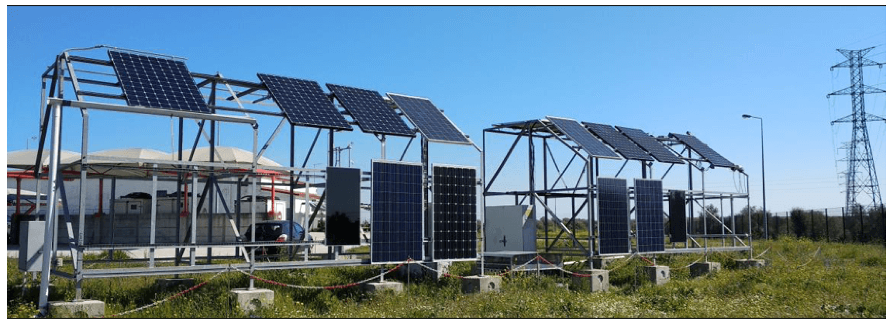
Within the EDP OPEN DATA initiative, there is a project named SunLAB (Figure 3), which conducts studies under real operating conditions in the field of photovoltaic production. This project helps explain the performance of different technologies in this area, providing support for decisions aimed at maximizing profitability in future investments. SunLAB facilitates the analysis and assessment of the viability of novel solutions, ideas, and technologies by encouraging the open exchange of operational data from EDP assets. This collaborative approach fosters innovation and the exploration of cleaner, more sustainable practices, potentially leading to the development of innovative solutions for the market.

The data used in this study were provided by the SunLAB project, and they consist of two data sets that separately present the production of photovoltaic modules from the SunLAB energy production station in Faro, as well as meteorological data from the same location for the year 2017. The data are organized in time series, acquired with a one-minute resolution and Coordinated Universal Time (UTC) timezone. The meteorological data set includes a daylight savings time correction, unlike the temperature and photovoltaic module production data, for which this correction is not present [18].

The photovoltaic module production data set comprises data from two different manufacturers (A and B), with each model having three orientations: vertical, optimal, and horizontal. The optimal orientation refers to the solar panel’s positioning to capture the maximum sunlight possible [19]. For each model, the provided data include the supplied power (W) and the panel temperature (°C).

The meteorological data set includes the following meteorological variables: ambient temperature (°C), indirect solar radiation (W/m²), direct solar radiation (W/m²), ultraviolet radiation (W/m²), wind speed (m/s), wind direction (°), precipitation (mm), and atmospheric pressure (hPa).

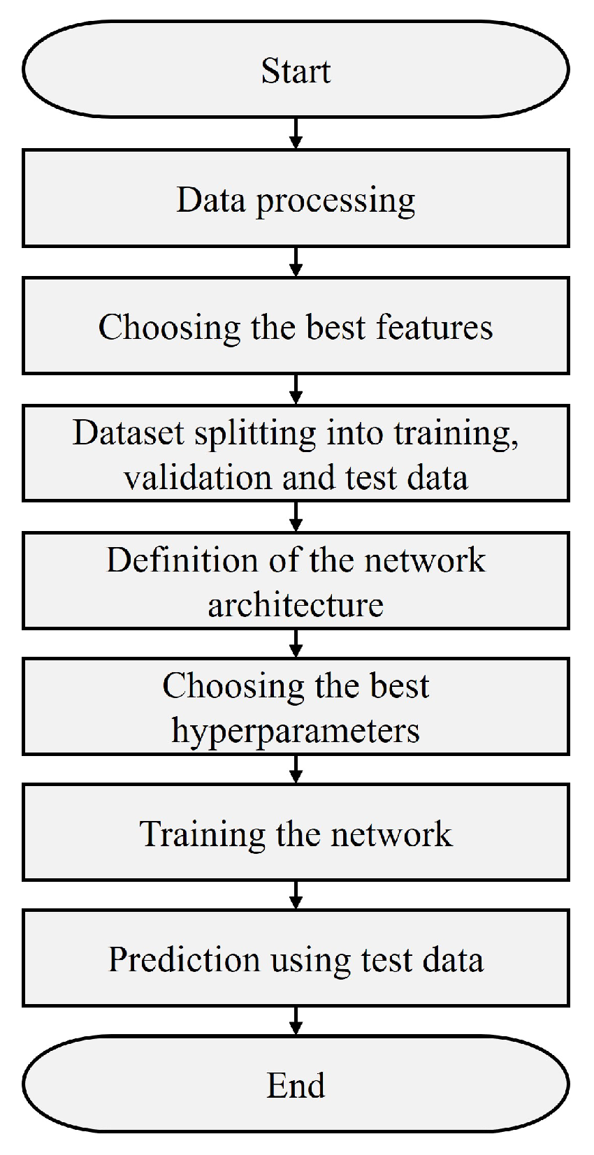
4. System Development

The goal of this work was to predict solar energy production with a 60-min horizon using meteorological data. The development of the system involved several steps (Figure 4). The first one was processing the data to determine which data should be considered for the model and which should be discarded. The selection of the best features representing the power generated via the solar panel was also crucial. Using too many features can slow down the process and result in inaccurate predictions. The data had to be divided into training, validation, and test sets. The training data was used to train the network, the validation data to evaluate the network’s generalization capability during training, and the test data to evaluate the network with unseen data after training. The network architecture consists of several LSTM layers and a DENSE layer, which is addressed later on. Choosing the hyperparameters for the neural network is also an important step. A network with a large size does not always yield good results, as will be seen in this section.

The system development was carried out in the Python programming language, version 3.7.16, using the Jupyter Notebook tool [20]. The Keras [21], TensorFlow [22], and Scikit-learn [23] libraries were used due to their good performance in implementing neural networks. To speed up network training, the NVIDIA RTX 4060 graphics card and the respective software, CUDA 11.2 and cuDNN 8.1, were employed.

4.1. Data Processing

4.1.1. Analyzing the Solar Energy Production Data Set

In the solar energy production data set, the module from manufacturer A in the optimal position was considered. After the data set was analyzed, it was found that there were missing power data, especially during the nighttime period. To address this gap, the missing data during the night were filled in with zero values, as there is no energy production during that time. Meanwhile, missing data during the daytime were filled in through interpolation. The minimum and maximum values were examined, and no outliers were found. The only observation was the presence of three power values near zero among much higher values. These values were replaced through interpolation.

4.1.2. Analyzing the Weather Station Data Set

Three outliers were identified in the ambient temperature and atmospheric pressure, and they were replaced using interpolation. No missing data were found in these variables.

4.1.3. Analysis after Integrating the Solar Energy Production and Weather Station Data Sets

After integrating the two data sets, it was found that there were missing power and panel temperature data on several days in the months of January, June, September, and November. All these days were excluded. Additionally, four data points were missing in all meteorological variables, and these were filled in using interpolation.

After the data processing, power and direct solar radiation curves were plotted, given their strong correlation. An example can be seen in Figure 5. It was noticed that, during daylight savings time, there was a constant deviation of approximately 1 h between these two variables. It was observed that one of the data sets had the daylight savings time correction, while the other did not. Therefore, the decision was made to remove the daylight savings time correction in order to eliminate this deviation. Furthermore, it was noted that, on 25 days between February and October, the maximum power of the solar panel was limited to around 180 W without a justifiable reason. Therefore, these days were also excluded.

4.2. Choosing the Best Features

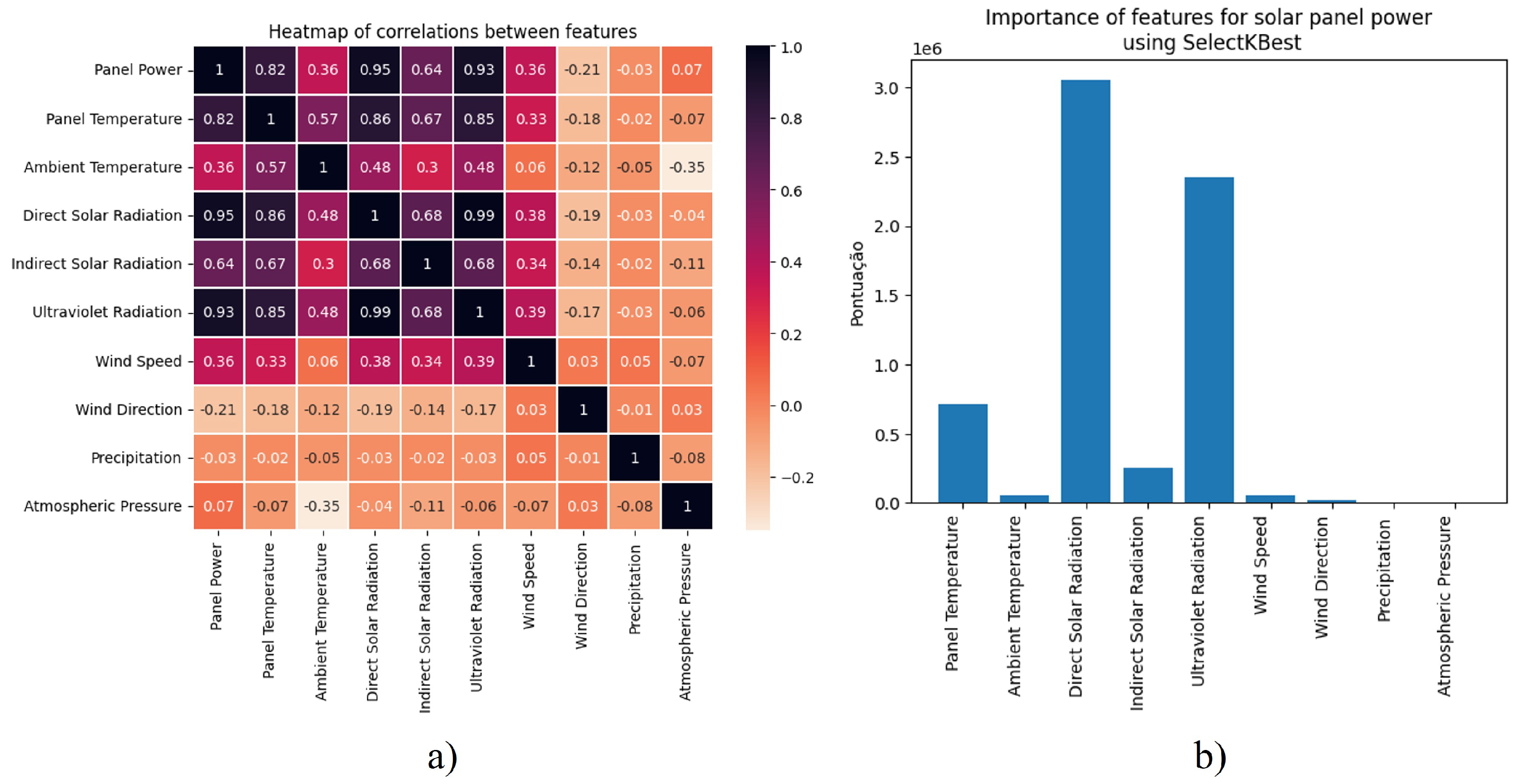
To identify the best features for the solar energy prediction model, we relied on the Pearson correlation matrix [24] and the SelectKBest method from scikit-learn [23], as shown in Figure 6a,b, respectively.

The Pearson correlation matrix measures the linear relationship between two quantitative variables, presenting values ranging from −1 (a perfect negative correlation) to +1 (a perfect positive correlation), reflecting the strength of a linear relationship between two sets of data. Values close to 0 indicate the absence of a linear relationship between the variables [24].

The SelectKBest method can be used to select the best features based on a statistical test. The univariate linear regression test “f_regression” was used, which returns the F-statistic and the p-value. Through this method, a bar chart was drawn in which a higher score indicates greater variable importance, as shown in Figure 6b [23].

By analyzing the charts in Figure 6, the top five variables that best represent the power generated via the solar system were selected: direct solar radiation, ultraviolet radiation, indirect solar radiation, wind speed, and ambient temperature. The temperature of the solar panel was not considered, ensuring that the solar energy production forecast depends exclusively on meteorological variables.

4.3. Data Set Division

The amount of daily solar radiation and other meteorological variables vary according to the season, as typically, solar exposure is higher during summer days compared to, for example, winter days [25]. Therefore, energy production forecasts were conducted for the four seasons of the year: winter, spring, summer, and autumn. The data set was divided into these four seasons, as presented in

Table 1. The time interval considered for each season.

Season	Considered Interval
Winter	1 January to 31 March
Spring	1 April to 30 June
Summer	1 July to 30 September
Autumn	1 October to 31 December

. We chose to consider a range between the first and last days of each month to simplify our implementation.

Each data set was split into training, validation, and test sets. The training and validation sets consist of the first 80% of the data for each data set, while the test set comprises the remaining 20%.

There are other approaches to data set splitting that can produce more reliable results, such as K-fold cross-validation. In this method, each data set is divided into k subsets (or “folds”), and the model is trained k times, using k−1 of these subsets as training data and the remaining subset as test data [26].

In [27], the author emphasized the importance of avoiding training a model with variables that have very different scales. Therefore, all variables in each data set were normalized using the “fit_transform” method of MinMaxScaler [23], ensuring that they fell within the range of 0 to 1. Normalizing the data ensured that all the variables had an equal impact during the model training.

4.4. Neural Network Architecture

For model training, the Adam optimizer [28] and the mean squared error (MSE) loss function were employed, a common choice for predictions involving LSTM [29].

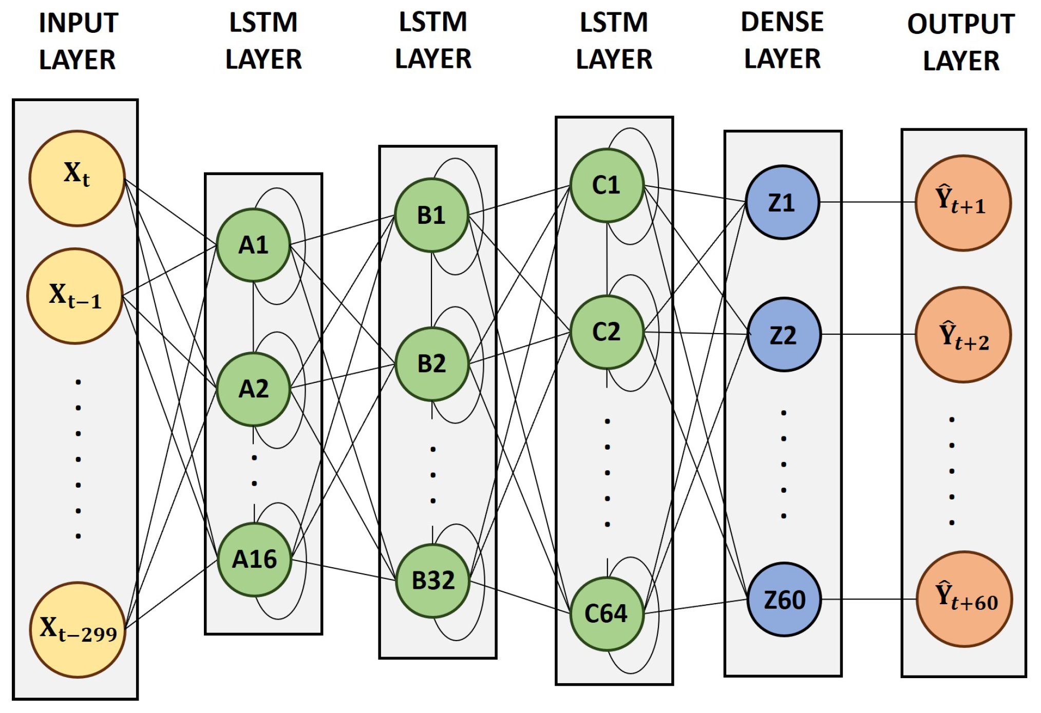
To prevent overfitting the LSTM network to the training data, dropout layers were added after the LSTM layers. Additionally, the EarlyStopping mechanism was implemented, which halts the training of the network if the loss function (MSE) does not decrease on the validation data over a certain number of epochs, as is defined in this section. Figure 7 depicts the architecture of the LSTM regression network used to predict solar energy production in each season of the year.

The network structure includes a sequence input layer composed of 300 values for each feature, representing values from the last 5 h. It is then followed by three hidden LSTM layers with 16, 32, and 64 neurons, respectively. After each LSTM layer, there is a dropout layer with a dropout percentage of 20%. The network structure concludes with a fully connected (DENSE) layer composed of 60 neurons, predicting the next 60 min of power.

4.5. Choosing the Best Hyperparameters

In

Table 2. Hyperparameters considered for the initial and final models.

	Initial Model	Final Model
Features	Direct Solar Radiation
	Indirect Solar Radiation
	Ultraviolet Radiation
	Ambient Temperature
	Wind Speed
Learning Rate	0.001	0.0001
Window Size	180	300
Prediction Window Size	60	60
Batch Size	128	128
Number of Training Epochs	350	350
Number of Epochs to Stop Training if validate loss does not decrease	100	100
Dropout Rate	0.2	0.2
Size and Number of LSTM Neurons	(64, 64, 64)	(16, 32, 64)
Size and Number of DENSE Neurons	60	60
DENSE Activation Function	Linear	ReLu
MAE	12.52	7.95
RMSE	28.37	18.97
R2	0.86	0.94

, hyperparameters and variables used in the initial and final models are presented. In the initial model, variables were chosen as described in Section 4.2, and hyperparameters were determined based on the results presented by the authors of the work [2] and through small experiments conducted using the Jupyter Notebook tool.

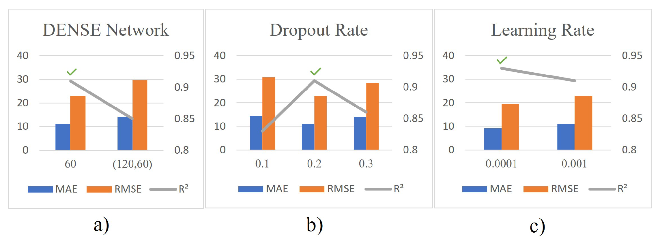
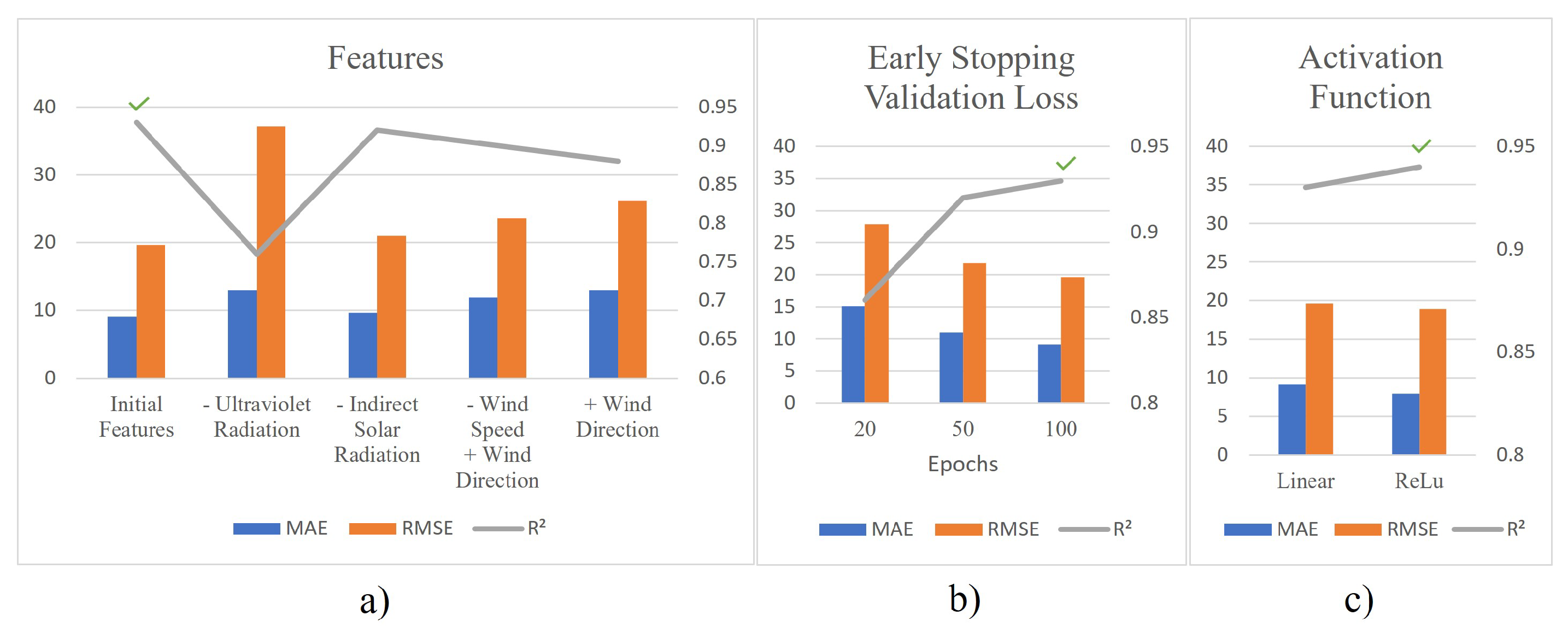
For the selection of hyperparameters for the final model, 20 models were trained with different configurations. For each model, performance indicators, namely MAE, RMSE, and R², were calculated based on test data and predictions. After the results were analyzed, as shown in Figure 8, Figure 9 and Figure 10, it was concluded that using a window size of 300 min, an LSTM network with three layers composed of 16, 32, and 64 neurons, and a learning rate of 0.0001 enabled the model to perform better.

The data set used to select the best model consisted of the first 10 days of the winter station-only data. Although it would be possible to obtain more accurate results using the entire data set for each season, this approach was not followed due to computer limitations, which would result in extended training times for each model. Despite not being used, there are online tools that provide faster model training, such as Google Colab [30].

5. Results

Four models were trained, one for each season of the year. The activation function chosen for the DENSE layer was Linear, as the use of the ReLU activation function did not yield good performance after the first model was trained. With the trained neural networks, it was possible to make power predictions with a horizon of 60 min using test data, i.e., data that the network had never seen. The results were analyzed for each season of the year, calculating the three performance indicators: MAE, RMSE, and R². The results are presented in

Table 3. Performance indicators for the prediction models of various seasons considering the test data using LSTM.

	Winter	Spring	Summer	Autumn
MAE	16.47	9.44	8.49	12.99
RMSE	31.18	19.76	18.03	30.78
R2	0.84	0.92	0.92	0.76

.

5.1. Interpretation of Performance Indicators

The winter network exhibited an MAE of 16.47, indicating an average absolute error of 16.47 units in the forecasts. The RMSE of 31.18 suggests considerable variation in errors, while an R² of 0.84 highlights that 84% of the power variation can be explained by the network. The spring network showed superior performance with an MAE of 9.44 and an RMSE of 19.76, indicating smaller average errors and less variation. An R² of 0.92 reveals a robust explanation of 92% of the variation in the test data. The summer network exhibited results similar to spring, with an MAE of 8.49, an RMSE of 18.03, and an R² of 0.92. Both seasonal networks efficiently explained the power variation. Finally, the autumn network showed slightly lower performance with an MAE of 12.99, an RMSE of 30.78, and an R² of 0.76. Although still a good fit, the autumn network showed slightly less explanation of the variation in the data compared to the spring and summer networks. In conclusion, the spring and summer networks stand out with superior performance, while the winter and autumn networks demonstrate satisfactory results, but with some differences in prediction accuracy and the ability to explain the variation in test data.

For each model, a training graph was generated during the network training, depicting the learning process of the network over epochs by showing the MSE values for both training data and validation data (Figure 11). Throughout the training of all models, a decrease in training errors (train loss) can be observed, confirming that the network’s learning process was successful. For the models of the spring and summer seasons (Figure 11b,c, respectively), the MSE for validation data is lower than the training data MSE, indicating that these models have a good generalization capability. The winter season model, shown in Figure 11a, exhibits an increasing validation loss with the progression of training epochs and was, therefore, stopped at around 100 epochs to prevent a decline in its generalizability. The autumn season model, depicted in Figure 11d, shows a slightly higher validation loss compared to the training data, but it remains relatively low, indicating good generalization as well.

5.2. Graphical Results for Forecasting Solar Energy Production

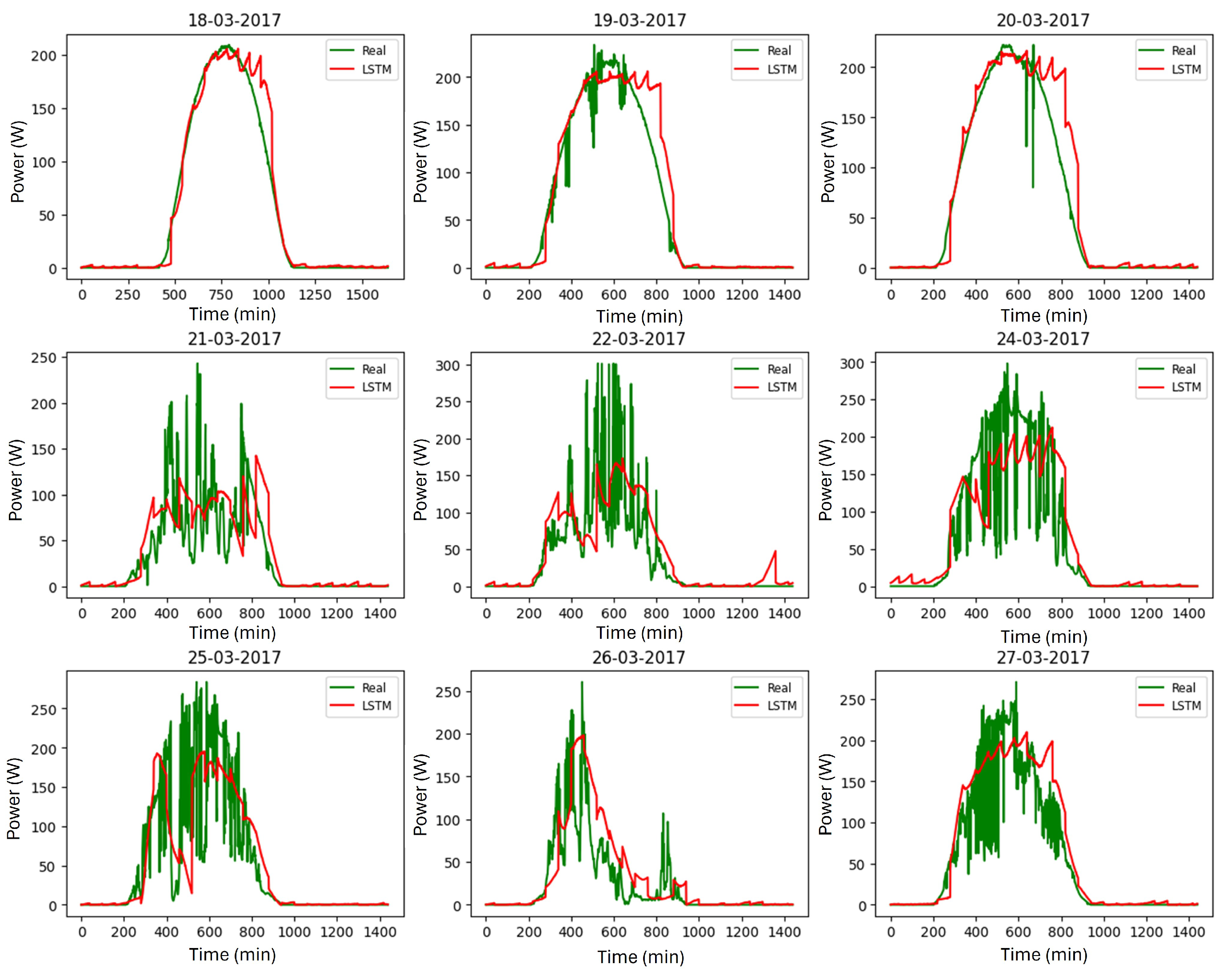
To evaluate the network’s performance, predictions of solar energy production were generated for several days that the network had never seen before (test data). In Figure 12, the prediction for the winter season between 18 March 2017 and 27 March 2017 is displayed. It was observed that the network can faithfully track the average value of the actual power. On days with significant power variation, between 21 March 2017 and 27 March 2017, the network accurately predicted the power waveform. The training data consisted mainly of days with high power variation, a typical characteristic of winter days [25]. Nevertheless, the network managed to predict energy production on days with lower power variation, showing a slight deviation between the predicted and actual power after reaching the maximum power.

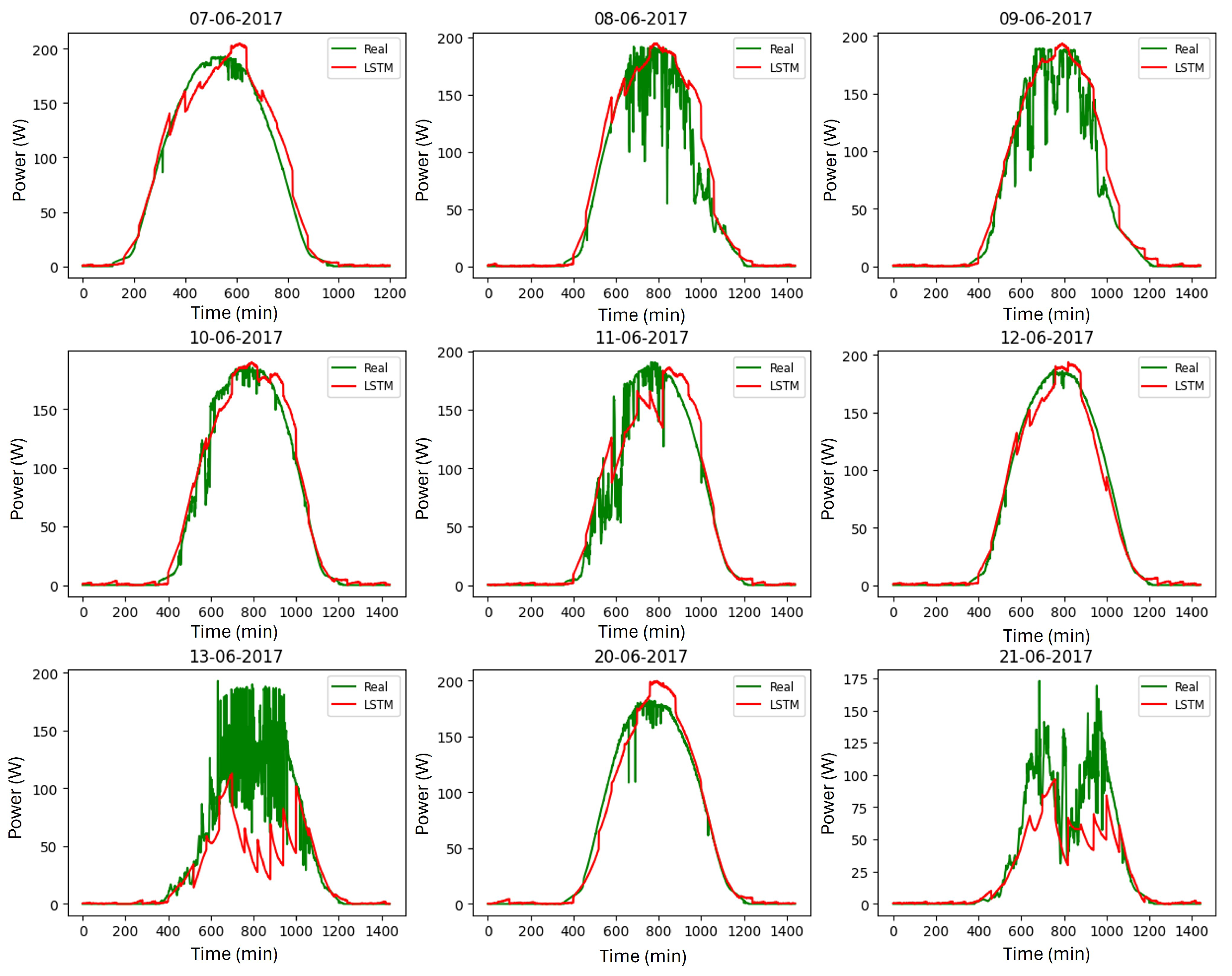
The prediction results for the autumn season, covering the period between 21 December 2017 and 29 December 2017, are presented in Figure 13. On days with low power variation, such as in the first three days, the prediction was quite accurate. On the days 24 December 2017 and 26 December 2017, there was a greater discrepancy between the actual and predicted values, but the network still managed to follow the same trend as the actual values. On the remaining days, the network closely tracked the average value of the actual power. The prediction results for the spring season, covering the period between 7 June 2017 and 21 June 2017, are presented in Figure 14. The prediction follows the average line of the actual power. On days with a higher power variation between 13 June 2017 and 21 June 2017, the network was also capable of accurately predicting energy production. The prediction results for the summer season, covering the period between 19 August 2017 and 29 August 2017, are presented in Figure 15. The prediction was very good, as it consistently followed the average line of the actual power on all days of the test data.

6. Comparison with Other Networks

The LSTM utilized in this work was compared with other networks, including BiLSTM, CNN, GRU, and RNN, each representing distinct approaches to applying neural networks for time series forecasting. The BiLSTM, GRU, and RNN networks have the same hyperparameters and architecture as the LSTM network. The CNN + LSTM network consists of the LSTM network from this work and a CNN network in parallel, in which the outputs are concatenated, and the prediction is made through the DENSE layer. The CNN network comprises three layers of one-dimensional convolution: (16, 5), (32, 3), and (64, 1) (number of kernels, kernel size).

The prediction results for each network for the test data are presented in

Table 4. Performance comparison of several models developed during the study.

Method	Season	MAE	RMSE	R2
BiLSTM	Winter	17.17	32.44	0.83
	Spring	9.31	19.22	0.91
	Summer	8.94	18.46	0.92
	Autumn	12.69	28.57	0.77
CNN	Winter	13.84	28.75	0.86
+LSTM	Spring	10.03	20.00	0.90
	Summer	12.12	19.74	0.88
	Autumn	12.31	27.50	0.75
GRU	Winter	14.27	30.42	0.85
	Spring	9.20	21.20	0.90
	Summer	7.98	17.13	0.93
	Autumn	11.05	26.87	0.78
RNN	Winter	15.71	30.78	0.86
	Spring	9.34	18.77	0.93
	Summer	8.44	15.90	0.94
	Autumn	11.99	27.31	0.80
LSTM	Winter	16.47	31.18	0.84
	Spring	9.44	19.76	0.92
	Summer	8.49	18.03	0.92
	Autumn	12.99	30.78	0.76

. For the BiLSTM method, an MAE ranging from 8.94 to 17.17 was observed, with lower values during the summer. Similarly, the RMSE ranged from 18.46 to 32.44, also showing lower values in the summer. The coefficient R² ranged from 0.77 to 0.92, with the maximum recorded during the summer. When the CNN method was analyzed, it was observed that the MAE and RMSE values were relatively lower during the summer, while the coefficient R² ranged from 0.75 to 0.90, reaching the highest value in the spring. The GRU method exhibited its best performance during the summer, with the lowest MAE 7.98 and RMSE 17.13 values. The coefficient R² ranged from 0.78 to 0.93, also being higher during the summer. Finally, the RNN method demonstrated its best results in the summer season, with lower values of MAE and RMSE. The coefficient R² ranged from 0.80 to 0.94, reaching its maximum during the summer.

The evaluated forecasting methods showed variable performance according to the season, with summer generally associated with more favorable prediction accuracy (lower values of MAE and RMSE and a higher R²). The GRU method stood out with the lowest mean absolute error during the summer, while the RNN method achieved the highest coefficient of determination R² during this season.

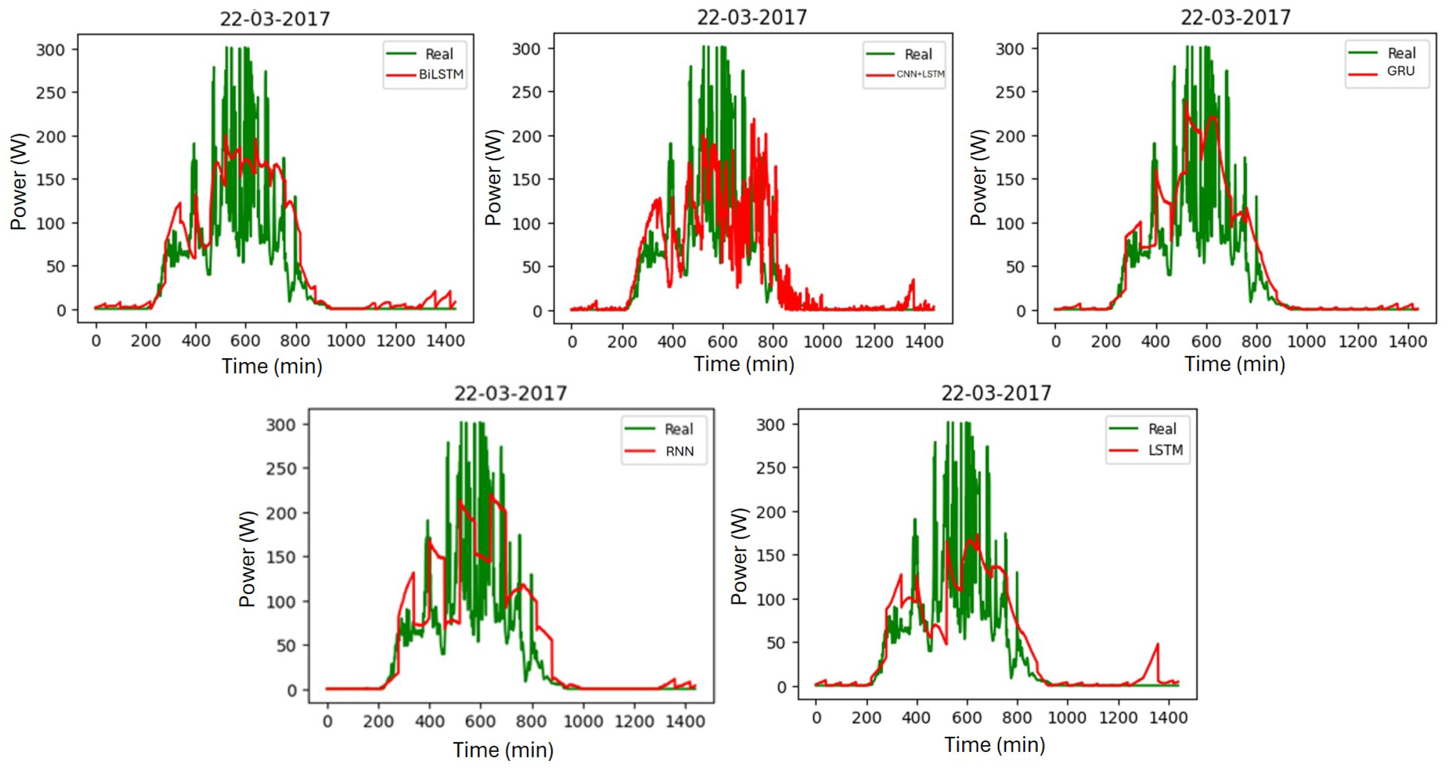
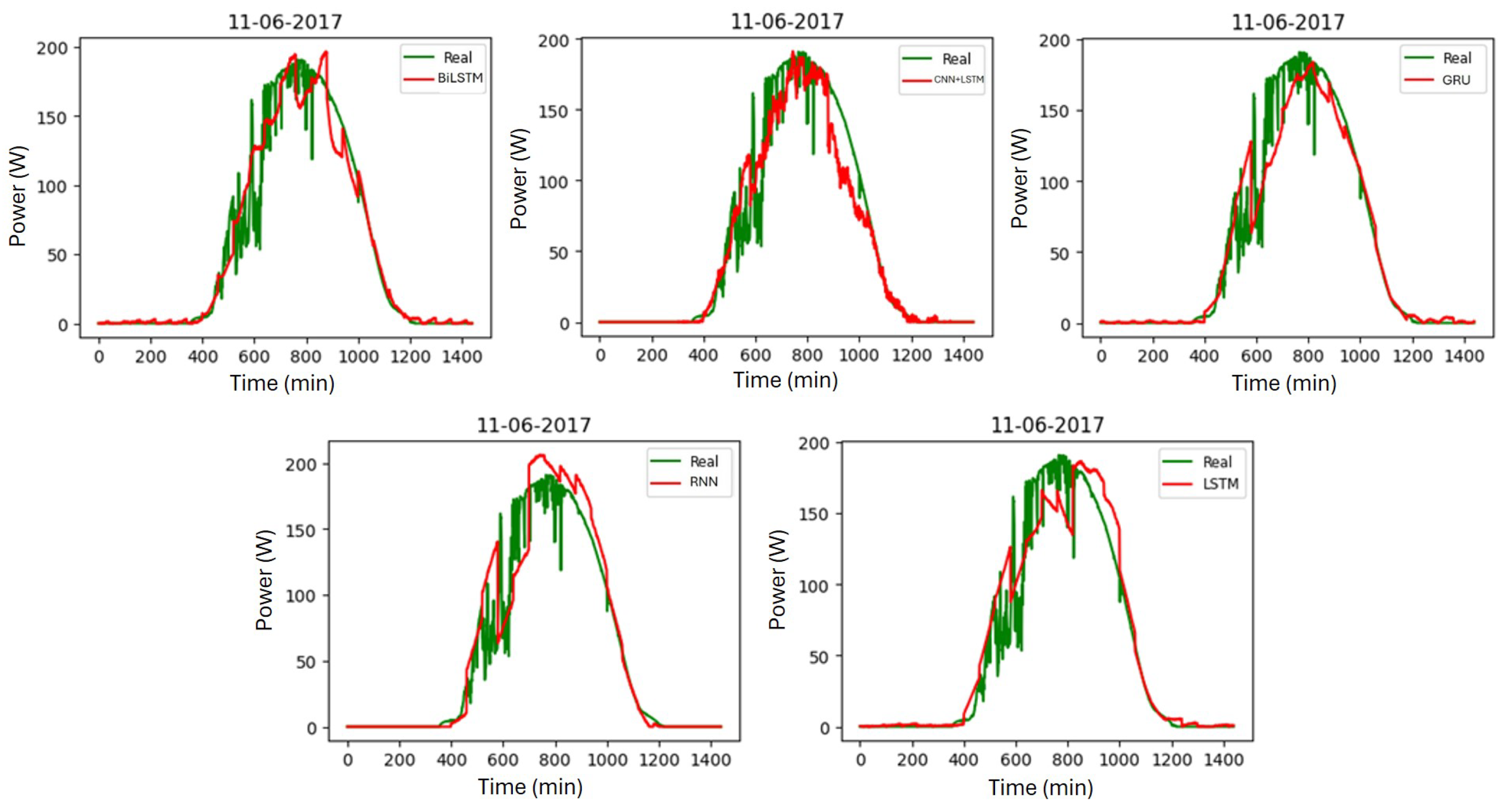
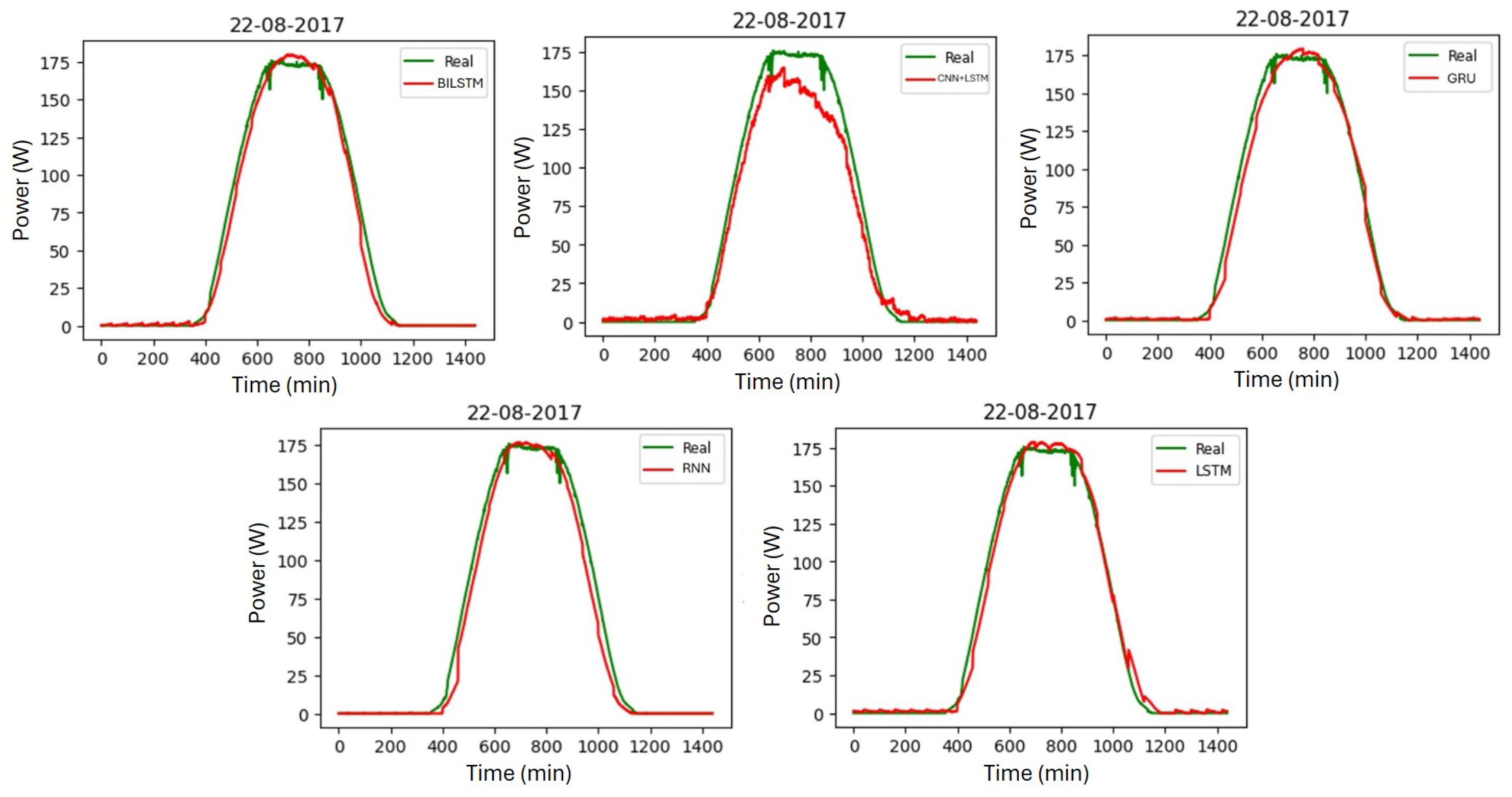
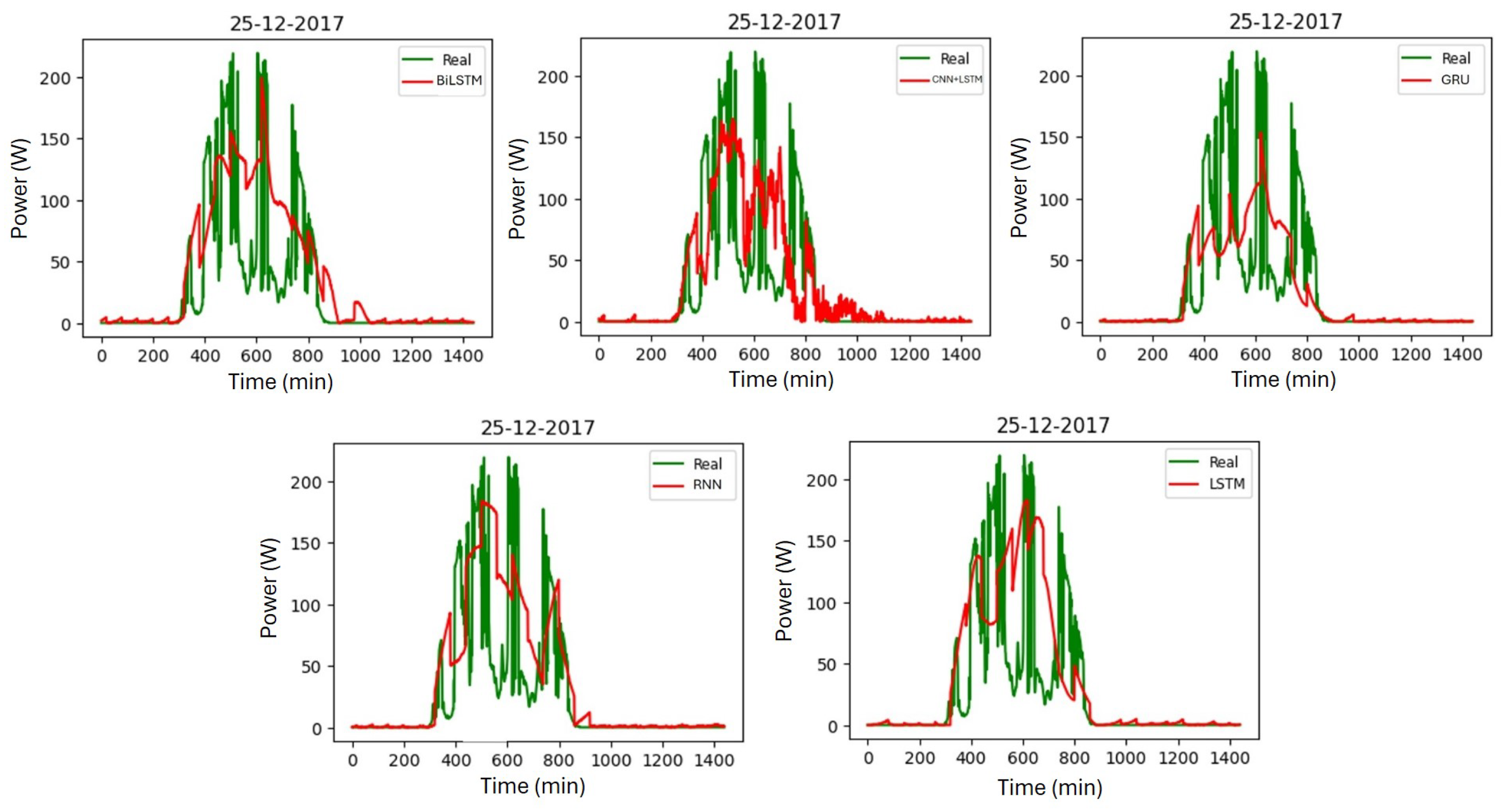
In Figure 16, Figure 17, Figure 18 and Figure 19, the results for one day of testing for the winter, spring, summer, and autumn seasons, respectively, are graphically presented. The CNN + LSTM network stands out, as there is a greater number of variations, while the other networks follow the average power value.

7. Conclusions

In Portugal, the use of renewable energies is increasingly prevalent today due to its significant potential for solar energy production [31]. In this context, it becomes crucial to anticipate the power that will be generated, allowing adjustments to the load and ensuring a better optimization of solar energy utilization.

By employing an LSTM network composed of only three layers, with 16, 32, and 64 neurons, respectively, it was possible to make predictions for solar energy production with a 60-min horizon. The exclusive use of meteorological variables has the advantage of allowing for the prediction of solar energy production without relying on the presence of the solar panel and all associated technology. This could be interesting to assess the feasibility of installing a solar panel in another location. The forecast could potentially yield even better results with a shorter horizon; however, this choice may not be as relevant, given the significant reduction in the forecast horizon. The models showed positive results, particularly standing out in the spring and summer seasons. The winter season also demonstrated satisfactory performance, followed by the autumn season. The main advantage of this network lies in its simplicity.

Looking ahead, future prospects could involve optimizing the hyperparameters of the models, taking into account the specific data set for each season. sunLAB has provided data since 2015, allowing for the inclusion of more information related to each season, which could result in a more refined adjustment of the network. Exploring more complex network architectures to improve generalization capabilities is a potential direction for future research.

References

1. Causes and Effects of Climate Change. Available online: https://www.un.org/en/climatechange/science/causes-effects-climate-change (accessed on 24 January 2024).
2. Dhaked, D.K.; Dadhich, S.; Birla, D. Power output forecasting of solar photovoltaic plant using LSTM. Green Energy Intell. Transp. 2023, 2, 100113. [Google Scholar] [CrossRef]
3. Rocha, H.R.; Fiorotti, R.; Fardin, J.F.; Garcia-Pereira, H.; Bouvier, Y.E.; Rodríguez-Lorente, A.; Yahyaoui, I. Application of AI for short-term pv generation forecast. Sensors 2023, 24, 85. [Google Scholar] [CrossRef]
4. Jailani, N.L.M.; Dhanasegaran, J.K.; Alkawsi, G.; Alkahtani, A.A.; Phing, C.C.; Baashar, Y.; Capretz, L.F.; Al-Shetwi, A.Q.; Tiong, S.K. Investigating the power of LSTM-based models in solar energy forecasting. Processes 2023, 11, 1382. [Google Scholar] [CrossRef]
5. Lateko, A.A.; Yang, H.T.; Huang, C.M. Short-term PV power forecasting using a regression-based ensemble method. Energies 2022, 15, 4171. [Google Scholar] [CrossRef]
6. Jlidi, M.; Hamidi, F.; Barambones, O.; Abbassi, R.; Jerbi, H.; Aoun, M.; Karami-Mollaee, A. An Artificial Neural Network for Solar Energy Prediction and Control Using Jaya-SMC. Electronics 2023, 12, 592. [Google Scholar] [CrossRef]
7. Alharkan, H.; Habib, S.; Islam, M. Solar Power Prediction Using Dual Stream CNN-LSTM Architecture. Sensors 2023, 23, 945. [Google Scholar] [CrossRef] [PubMed]
8. Mahesh, B. Machine learning algorithms-a review. Int. J. Sci. Res. (IJSR) 2020, 9, 381–386. [Google Scholar]
9. Jung, S.M.; Park, S.; Jung, S.W.; Hwang, E. Monthly electric load forecasting using transfer learning for smart cities. Sustainability 2020, 12, 6364. [Google Scholar] [CrossRef]
10. Svozil, D.; Kvasnicka, V.; Pospichal, J. Introduction to multi-layer feed-forward neural networks. Chemom. Intell. Lab. Syst. 1997, 39, 43–62. [Google Scholar] [CrossRef]
11. Albawi, S.; Mohammed, T.A.; Al-Zawi, S. Understanding of a convolutional neural network. In Proceedings of the 2017 International Conference on Engineering and Technology (ICET), Antalya, Turkey, 21–23 August 2017; pp. 1–6. [Google Scholar]
12. Lipton, Z.C.; Berkowitz, J.; Elkan, C. A critical review of recurrent neural networks for sequence learning. arXiv 2015, arXiv:1506.00019. [Google Scholar]
13. Chang, R.; Bai, L.; Hsu, C.H. Solar power generation prediction based on deep learning. Sustain. Energy Technol. Assess. 2021, 47, 101354. [Google Scholar] [CrossRef]
14. Colah, C. Understanding LSTM Networks. Available online: https://colah.github.io/posts/2015-08-Understanding-LSTMs/ (accessed on 4 February 2024).
15. Yu, Y.; Si, X.; Hu, C.; Zhang, J. A review of recurrent neural networks: LSTM cells and network architectures. Neural Comput. 2019, 31, 1235–1270. [Google Scholar] [CrossRef] [PubMed]
16. Agrawal, R. Know the Best Evaluation Metrics for Your Regression Model! Available online: https://www.analyticsvidhya.com/blog/2021/05/know-the-best-evaluation-metrics-for-your-regression-model/ (accessed on 20 December 2023).
17. de Myttenaere, A.; Golden, B.; Le Grand, B.; Rossi, F. Mean Absolute Percentage Error for regression models. Neurocomputing 2016, 192, 38–48. [Google Scholar] [CrossRef]
18. EDP Open Data. Available online: https://www.edp.com/en/innovation/open-data/data (accessed on 4 January 2024).
19. Mirzabekov, S. Method of orientation of solar panels of solar power plant. In Proceedings of the E3S Web of Conferences, Tashkent, Uzbekistan, 26–28 April 2023; EDP Sciences. Volume 401, p. 04018. [Google Scholar]
20. Randles, B.M.; Pasquetto, I.V.; Golshan, M.S.; Borgman, C.L. Using the Jupyter Notebook as a Tool for Open Science: An Empirical Study. In Proceedings of the 2017 ACM/IEEE Joint Conference on Digital Libraries (JCDL), Toronto, ON, Canada, 19–23 June 2017; pp. 1–2. [Google Scholar]
21. Arnold, T.B. kerasR: R Interface to the Keras Deep Learning Library. J. Open Source Softw. 2017, 2, 296. [Google Scholar] [CrossRef]
22. Pang, B.; Nijkamp, E.; Wu, Y.N. Deep learning with tensorflow: A review. J. Educ. Behav. Stat. 2020, 45, 227–248. [Google Scholar] [CrossRef]
23. Bisong, E. Building Machine Learning and Deep Learning Models on Google Cloud Platform; Springer: Berlin/Heidelberg, Germany, 2019. [Google Scholar]
24. Belorkar, A.; Guntuku, S.C.; Hora, S.; Kumar, A. Interactive Data Visualization with Python: Present Your Data as an Effective and Compelling Story; Packt Publishing Ltd.: Birmingham, UK, 2020. [Google Scholar]
25. Climate and Average Weather Year Round in Calendário Portugal. Available online: https://weatherspark.com/y/32466/Average-Weather-in-Calend%C3%A1rio-Portugal-Year-Round (accessed on 27 January 2024).
26. Anguita, D.; Ghelardoni, L.; Ghio, A.; Oneto, L.; Ridella, S. The ‘K’ in K-fold Cross Validation. In Proceedings of the ESANN, Bruges, Belgium, 25–27 April 2012; pp. 441–446. [Google Scholar]
27. Chollet, F. Deep Learning with Python, 2nd ed.; Manning: Shelter Island, NY, USA, 2021. [Google Scholar]
28. Kingma, D.; Ba, J. Adam: A Method for Stochastic Optimization. In Proceedings of the International Conference on Learning Representations (ICLR), San Diego, CA, USA, 7–9 May 2015. [Google Scholar]
29. Qing, X.; Niu, Y. Hourly day-ahead solar irradiance prediction using weather forecasts by LSTM. Energy 2018, 148, 461–468. [Google Scholar] [CrossRef]
30. Google Colab—Online Interactive Notebook Environment. Available online: https://colab.research.google.com/ (accessed on 12 February 2024).
31. Global Solar Atlas. Available online: https://globalsolaratlas.info/map (accessed on 5 February 2024).
Figure 1. (a) Neural network composed of an input layer, two fully connected hidden layers (DENSE), and an output layer. (b) Constitution of an artificial neuron.
Energies 17 02582 g001
Figure 2. Architecture of an LSTM cell [15].
Energies 17 02582 g002
Figure 3. Weather and solar energy production station of SunLab located in Faro, Portugal [18].
Energies 17 02582 g003
Figure 4. Block diagram of system development.
Energies 17 02582 g004
Figure 5. Power and direct solar radiation charts for 22–23 January 2017.
Energies 17 02582 g005
Figure 6. Choice of the best features for the model: (a) Pearson correlation matrix and (b) SelectKBest method from the scikit-learn library.
Energies 17 02582 g006
Figure 7. Architecture of the final model’s neural network without representing the dropout layers.
Energies 17 02582 g007
Figure 8. Variation in hyperparameters considering the initial setup and a window size of 300: (a) variation in the window size, (b) variation in the batch size, and (c) variation in the number of layers and neurons in the LSTM network.
Energies 17 02582 g008
Figure 9. Variation in hyperparameters considering the initial setup, a window size of 300, and LSTM layers with 16, 32, and 64 neurons: (a) variation in the number of layers and neurons in the DENSE network, (b) variation in the dropout rate, and (c) variation in the learning rate.
Energies 17 02582 g009
Figure 10. Variation in hyperparameters considering the initial setup, a window size of 300, LSTM layers with 16, 32, and 64 neurons, and a learning rate of 0.0001: (a) input variables (− means to remove, and + means to add), (b) variation in the number of epochs to stop training if the validation loss does not decrease, and (c) activation function used in the DENSE layer.
Energies 17 02582 g010
Figure 11. Evolution of the mean squared error (MSE) based on training data and validation data during the training of the network: (a) winter season, (b) spring season, (c) summer season, and (d) autumn season.
Energies 17 02582 g011
Figure 12. Power prediction for the first nine days of the test data during the winter season with a 60 min horizon.
Energies 17 02582 g012
Figure 13. Power prediction for the first nine days of the test data during the autumn season with a 60 min horizon.
Energies 17 02582 g013
Figure 14. Power prediction for the first nine days of the test data during the spring season with a 60 min horizon.
Energies 17 02582 g014
Figure 15. Power prediction for the first nine days of the test data during the summer season with a 60 min horizon.
Energies 17 02582 g015
Figure 16. Power forecast using BiLSTM, CNN + LSTM, GRU, RNN, and LSTM neural networks for one day of testing in the winter season.
Energies 17 02582 g016
Figure 17. Power forecast using BiLSTM, CNN + LSTM, GRU, RNN, and LSTM neural networks for one day of testing in the spring season.
Energies 17 02582 g017
Figure 18. Power forecast using BiLSTM, CNN + LSTM, GRU, RNN, and LSTM neural networks for one day of testing in the summer season.
Energies 17 02582 g018
Figure 19. Power forecast using BiLSTM, CNN + LSTM, GRU, RNN, and LSTM neural networks for one day of testing in the autumn season.
Energies 17 02582 g019