Rapid Design Method of Heavy-Loaded Propeller for Distributed Electric Propulsion Aircraft

Abstract

On Distributed Electric Propulsion (DEP) aircraft, the deployment of numerous high-lift propellers with small diameters on the wing’s leading edge significantly enhances lift during low-speed flight. The increase in the number of propellers leads to a decrease in diameter, which increases the disc loading. In this paper, a rapid design method applicable to heavy-loaded propellers is developed and does not require iterative calculations compared to traditional heavy-loaded propeller design methods, enabling rapid completion of the propeller design. The results of CFD computation show that the relative thrust error of the method proposed in this paper is within 5% for disc loading ranging from 600 Pa to 1400 Pa, features a high-accuracy design of propellers with required thrust, and high thrust coefficients are achieved within large advance ratio range.

1. Introduction

The demand for reducing carbon dioxide emissions in air transportation has led to a growing interest in aircraft equipped with electric propulsion systems. Distributed Electric Propulsion (DEP) is a kind of technology that uses multiple electric motors and propellers distributed across an aircraft’s wing or body to provide propulsion to improve aero-propulsion efficiency, reduce noise, and enhance aircraft performance.

There are two types of propellers installed on the wing of a DEP aircraft: cruise propellers on the wing tip and high-lift propellers on the leading or trailing edge of the wing. Wingtip-mounted propellers installed in a tractor configuration can decrease the wing-induced drag due to their ability to effectively weaken wingtip vortices [1]. The placement of several electric motors driving individual tractor propellers spaced along each wing helps to increase dynamic pressure, reduce stall speed, and eliminate the need for the placement of complex high-lift devices on the trailing edge of each wing, which are necessary for traditional aircraft [2]. Under the influence of propeller slipstream, the lift can increase significantly by 60%, though the propulsive efficiency decreases by 19% according to Beckers’ research [3]; the closer the propellers spaced spanwise, the lower the stall speed [3,4].

Using smaller-diameter propellers can generate higher propeller-induced velocities over the entire wing surface than using fewer propellers with the same total power [5]. For example, the propellers used for NASA’s X57 have been changed from the P2600T’s two propellers with a diameter of 1.78 m to 12 high-lift propellers with a diameter of 1.89 feet and 2 wingtip-mounted cruise propellers with a diameter of 5 feet [6,7]. Propellers with smaller diameters placed ahead of the wing’s leading edge are generally favored because they generate reduced thrust for an equivalent increase in axial velocity over the wing [8]. Moreover, propeller noise can be reduced if the propeller radius decreases [9]. The small propeller radius results in a heavy-loaded propeller.

To reduce the total power consumption of the DEP system, the required thrust of propellers spaced on the leading edge and tip of each wing is different [10], which increases the propeller design efforts.

The development of propeller design theory first originated from marine propeller design. In 1865, Rankine [11] developed a theory of marine propellers, which is the first theory related to propellers. Betz [12] and Goldstein [13] carried out propeller design research based on minimum energy loss. In 1948, Theodorsen [14] demonstrated that the Betz condition with minimum energy loss can also be applied to heavy disc loading. In 1979, Larrabee [15] proposed a new design method based on Betz conditions and light loading assumption, assuming that the axial velocity displacement relative to the axial flow velocity of the propeller is small. In 1983, Adkins et al. [16] improved the design methodology by eliminating the small angle approximation and some of the light loading approximations in classical propeller design theory and completed the design of medium loaded propeller by iterative computation. The work of the scholars mentioned above laid the foundation for modern propeller design theory.

In 2016, Traub et al. [17] proposed a simplified design method and compared its results with the Adkins and Liebeck method. The designed thrust for the compared propeller is 1000 N, with a blade radius of $3.048$ m. The results indicate that the proposed method and Adkins and Liebeck’s method yield similar shapes, with longer chord inboard and shorter chord outboard. The estimated pitch distributions of both methods are essentially identical. To conduct heavy-loaded propeller design for DEP aircraft, Patterson et al. [18,19] proposed a simple method for a high-lift propeller conceptual design method based on blade element momentum theory (BEMT). The high-lift propeller of NASA’s X57 (215N gross thrust at design condition) was designed based on this approach. However, due to the modification to the desired axial induction factor near the hub, this method will not produce exactly the desired results, and approximately 2–3 iterations are required for convergence, according to Patterson’s practice. Based on the blade element theory and the momentum theory, Fan et al. [20,21] proposed a rapid propeller inverse design method suitable for DEP aircraft, yet this method requires the prescribed circulation distribution of the blades. Xue et al. [22] proposed an inverse aerodynamic design for a DEP propeller based on the desired propeller slipstream. This method requires iterative execution to achieve the desired propeller that meets the requirements. For heavy-loaded propeller design for distributed electric propulsion aircraft, modifications are typically made based on the BEMT to meet design requirements through iterative design, therefore extending the time required for the design process.

This paper will first introduce the design method of a light-loaded propeller based on the Betz condition and then propose a rapid design method applicable to heavy-loaded propellers to improve the design accuracy with the required thrust. This new method eliminates the necessity for iterative computations across multiple design steps, ensuring rapid completion of the design. The design result is then verified by the CFD analysis, which proves the reliability of the design method proposed in this paper.

2. Materials and Methods

As shown in Figure 1, the propeller disc loading is defined as

$$dc=\frac{T}{A}=\frac{T}{\pi R_t^2}$$

(1)

where T is the propeller thrust, $R_t$ is the propeller tip radius and A is the propeller disc area.

There is no clear boundary between light-loaded propellers and heavy-loaded propellers. A light-loaded propeller means that the induced velocities(both in axial and tangential directions) are small relative to the magnitude of the freestream velocities. According to our design practice, when the blade loading is less than 200 Pa, it can be considered that the above requirement holds true.

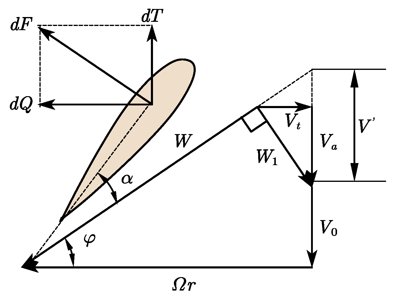
2.1. Design Method of Light Loaded Propeller Based on Betz Condition

Figure 2 shows the force analysis of the blade element under the light loading assumption. In Figure 2, $\alpha$ is the angle of attack of the blade element, $\phi$ is the actual inflow angle. W is the total velocity, $W_1$ is the induced velocity, $V_a$ is the axial-induced velocity, $V_t$ is the tangential-induced velocity, and $V^{\prime }$ is the axial velocity displacement. $dT$ is the thrust, and $dQ$ is the tangential force of the blade element.

Under the light loading assumption, the induced velocity $W_1$ is perpendicular to the total velocity W, and the $V_a$, $V_t$ and $\phi$ can be obtained as:

$$V_a=V^{\prime }{cos}^2\phi$$

(2)

$$V_t=V^{\prime }cos\phi sin\phi$$

(3)

$$tan\phi =\frac{V_0+V_a}{\Omega r-V_t}=\frac{V_0+V^{\prime }}{\Omega r}$$

(4)

According to vortex theory, the relationship between the circulation at the propeller disc and the tangential-induced velocity is

$$\Gamma =\frac{4\pi r}{N_b}Vt$$

(5)

and the thrust of the blade element:

$$dT=\rho \Gamma (r,V)(\Omega r-V_t)dr$$

(6)

By combining Equations (2)–(6), the blade element thrust can be obtained as:

$$dT=f\frac{4\pi r\rho }{N_{\mathrm{b}}}\left(V_0+V^{\prime }{cos}^2\phi \right)V^{\prime }{cos}^2\phi dr$$

(7)

where f is the Prandtl’s correction factor

$$f=\frac{2}{\pi }arccos{\mathrm{e}}^{-\frac{N_b(R-r)}{2rtan\phi }}$$

(8)

so the thrust of a single blade can be obtained by integrating Equation (7) from the hub to the tip as below:

$$T={\int }_{R_{hub}}^{R_{tip}}f\frac{4\pi r\rho }{N_b}\left(V_0+V^{\prime }{cos}^2\phi \right)V^{\prime }{cos}^2\phi dr$$

(9)

With the given flight altitude, the air density can be obtained from the International Standard Atmosphere (ISA) [23]. If the flight velocity $V_0$, rotational speed $\Omega$, number of propeller blades $N_b$, radius of propeller tip and hub are given, the blade element thrust will be determined by the axial velocity displacement by substituting Equation (4) and Equation (8) into Equation (7).

The distribution of axial velocity displacement $V^{\prime }$ along the radial direction of the blade should be constant so that the maximum efficiency of propeller can be achieved under the given thrust according to Betz condition [12,16], Therefore, the propeller thrust should be a function of the axial velocity displacement $V^{\prime }$. The axial velocity displacement can be obtained by solving Equation (9) with nonlinear algorithms such as Newton iteration.

For each section, $\phi$ can be obtained after the previously obtained axial velocity displacement is substituted into Equation (4), and the tangential-induced velocity $V_t$ can be obtained by Equation (3), then the optimal circulation distribution based on the light loading assumption can be obtained from Equation (5).

The blade element thrust $dT$ and torque $dQ$ are

$$dT=\frac{1}{2}\rho W^{2}b\left(c_{l}cos\phi -c_{d}sin\phi \right)dr$$

(10)

$$dQ=\frac{1}{2}\rho W^{2}b\Omega \left(c_{l}sin\phi +c_{d}cos\phi \right)rdr$$

(11)

where $c_l$ and $c_d$ are the lift and the drag coefficient of the airfoil, respectively, and the thrust and torque of a single blade under design conditions can be obtained by integrating Equations (10) and (11) from the hub to the tip.

The total velocity W and the induced velocity $W_1$ can be assumed to be perpendicular to each other under light loading assumption so that the relationship between the thrust and the axial velocity displacement on a given design point can be obtained. The axial velocity displacement can be derived based on the conclusion that the axial velocity displacement of each section is the same at the minimum energy loss [12], and the axial and tangential-induced velocities can be further calculated, and thus the design of the blade can be ultimately completed.

2.2. Rapid Design Method for Heavy Loaded Propellers

When the propeller thrust remains constant, the disc loading will increase if the propeller radius is reduced. In the method based on the Betz condition, it is necessary to ensure that the propeller disc loading is small to minimize the error resulting from the assumption that the induced velocity $W_1$ is perpendicular to the total velocity W. As indicated in Figure 3, $W_1$ and W are not perpendicular to each other as the disc loading increases, then Equations (2)–(4) cannot be derived. Therefore, the method based on the Betz condition cannot be used for heavy-loaded propeller design.

To solve this problem, a novel method applicable to heavy-loaded propeller design is proposed in this paper. The main idea of this method is to calculate the axial velocity displacement based on the optimal circulation distribution with finite blades, considering the position of the blade hub and establishing the relationship between induced velocity and propeller thrust. In this method, there is no need to consider the relationship between $W_1$ and W, thus avoiding the assumption of light disc loading.

According to the vortex theory, the relationship between circulation $\Gamma$ and tangential-induced velocity $V_t$ is

$$\Gamma =\frac{4\pi r}{N_b}{V}_t$$

(12)

The optimal circulation distribution considering the position of the propeller hub and the finite blades [24] is

$$\Gamma \left(r,V^{\prime }\right)=\left[{\Gamma }_{infinite}\left(r,V^{\prime }\right)+{\Gamma }_{infinite}\left(\frac{R_{hub}^2}{r},V^{\prime }\right)-{\Gamma }_{infinite}\left(R_{hub},V^{\prime }\right)\right]\ast F$$

(13)

where $R_{hub}$ is the radius of the propeller hub, and ${\Gamma }_{infinite}$ is the optimal circulation of an infinite span blade, which is defined as

$${\Gamma }_{infinite}\left(r,V^{\prime }\right)=\frac{2\pi V_0{V}^{\prime }}{2\pi n_s{N}_b}·\frac{x^2}{1+x^2}$$

(14)

where $n_s$ is the rotational velocity (rev/s) and x is the reciprocal of the local advance ratio,

$$x=\frac{2\pi n_{s}r}{V_0}$$

(15)

F in Equation (13) is the other form of the Prandtl’s correction factor,

$$F=\frac{2}{\pi }\mathrm{arc}cos\left(e^{-f}\right)$$

(16)

where

$$f=\frac{N_b}{2}\frac{R_{tip}-r}{R_{tip}}\frac{\sqrt{1+J^2}}{J}$$

(17)

and J is the advance ratio, i.e.,

$$J=\frac{V_0}{2\pi n_{s}R}$$

(18)

According to Equations (16) and (17), the Prandtl’s correction factor F at the blade tip is zero, and the optimal circulation at the blade tip is determined as $\Gamma =0$, resulting in a chord length of zero. To solve this problem, cubic splines are used to interpolate the radial section and circulation distribution of 5 sections near the blade tip, and the interpolation function is used to obtain the circulation at the blade tip.

The blade element thrust

$$dT=\rho \Gamma \left(r,V^{\prime }\right)\left(\Omega r-V_t\right)dr$$

(19)

and from Equation (12), we have

$$V_t=\frac{\Gamma \ast N_b}{4\pi r}$$

(20)

The Equations (19) and (20) are combined as follows:

$$dT=\rho \Gamma \left(r,V^{\prime }\right)\left(\Omega r-\frac{N_b\Gamma \left(r,V^{\prime }\right)}{4\pi r}\right)dr$$

(21)

and the propeller thrust can be calculated as

$$T={\int }_{R_{hub}}^{R_{tip}}\rho \Gamma \left(r,V^{\prime }\right)\left(\Omega r-\frac{N_b\Gamma \left(r,V^{\prime }\right)}{4\pi r}\right)dr=H\left(V^{\prime }\right)$$

(22)

As shown in Equation (22), with the given number of blades, blade tip radius, hub radius, rotational velocity, and air density, the propeller thrust is a function of the axial velocity displacement $V^{\prime }$, which can be solved through iterative computation for the required thrust.

Since we solve the axial velocity displacement $V^{\prime }$ from Equation (22), then the inflow angle $\phi$ between the incoming flow and the disc plane can be determined by

$$\phi =\mathrm{arc}tan\frac{V_0+V^{\prime }}{\Omega r}$$

(23)

The total velocity

$$W=\sqrt{{\left(V_0+V^{\prime }\right)}^2+{\left(\Omega r\right)}^2}-\frac{V_t}{cos\phi }$$

(24)

and the axial-induced velocity

$$V_a=V^{\prime }-V_{t}tan\phi$$

(25)

According to the Kutta–Joukowski theorem, the lift of the blade element

$$dL=\rho \Gamma \left(r\right)Wdr$$

(26)

and the lift of the blade element can also be written as:

$$dL=\frac{1}{2}\rho W^2{c}_{l}bdr$$

(27)

The Equations (26) and (27) are combined as follows:

$$\Gamma =\frac{1}{2}W{c}_{l}b$$

(28)

The pitch angle of the blade can be obtained as

$$\theta =\phi +\alpha$$

(29)

For a given airfoil, $\alpha$ is the angle of attack with a maximum lift-to-drag ratio. In this paper, XFOIL version 6.99 [25] is used to calculate the aerodynamic performance of airfoils.

After the blade design is completed, the thrust and torque of each blade element can be calculated based on parameters such as inflow angle, angle of attack, chord length, velocity, etc., according to Equations (10) and (11).

The summary of the rapid design process applicable to heavy-loaded propellers, based on the above derivation, can be outlined as follows:

• Give the design requirements, including specified thrust requirement T, flight speed $V_0$, number of blades $N_b$, rotational velocity $n_s$, tip radius $R_t$, hub radius $R_h$ and the atmospheric density $\rho$.
• Solve for the axial velocity displacement $V^{\prime }$ according to Equation (22).
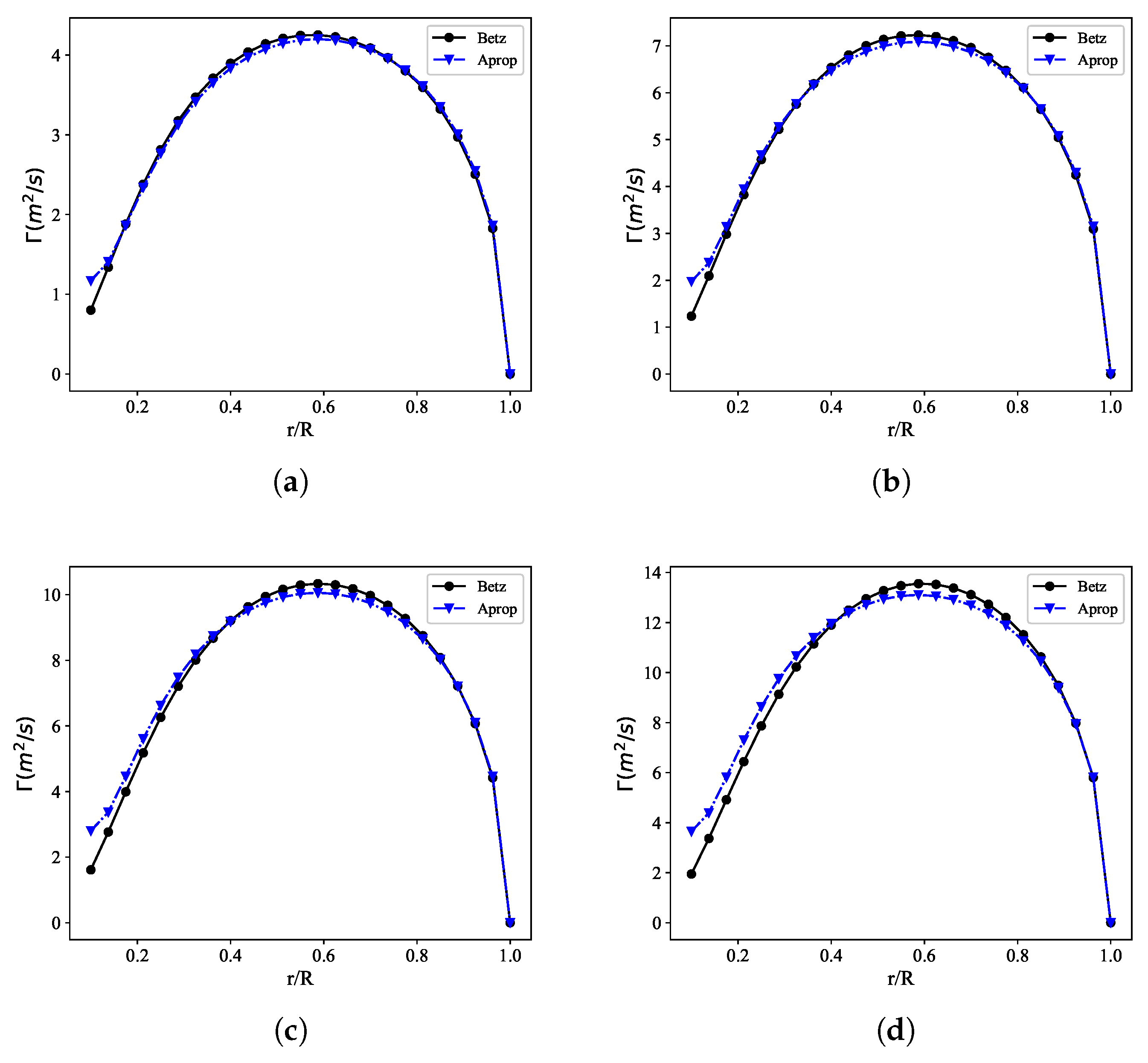
• Determine the optimal circulation distribution $\Gamma$ at each section according to Equation (13).
• Perform cubic spline interpolation on the circulation of sections other than the blade tip, and then perform extrapolation based on the obtained interpolation functions to obtain the circulation at the blade tip to avoid this circulation being zero.
• Determine the actual inflow angle $\phi$ at each section according to Equation (23).
• Obtain the tangential-induced velocity $V_t$ at each section according to Equation (20).
• Calculate the total velocity W at each section according to Equation (24)
• Assume a certain value for the lift coefficient at each section (selected based on the airfoil) and calculate the initial chord length b at each section according to Equation (28).
• Compute the aerodynamic characteristics of the given airfoil at a specified Reynolds number and Mach number using aerodynamic tools such as XFOIL [25] according to the chord length calculated in the previous step. Identify the optimum angle of attack $\alpha$ and its corresponding lift coefficient $c_l$.
• Substitute the $c_l$ obtained in step 9 into Equation (28) to update the chord length b.
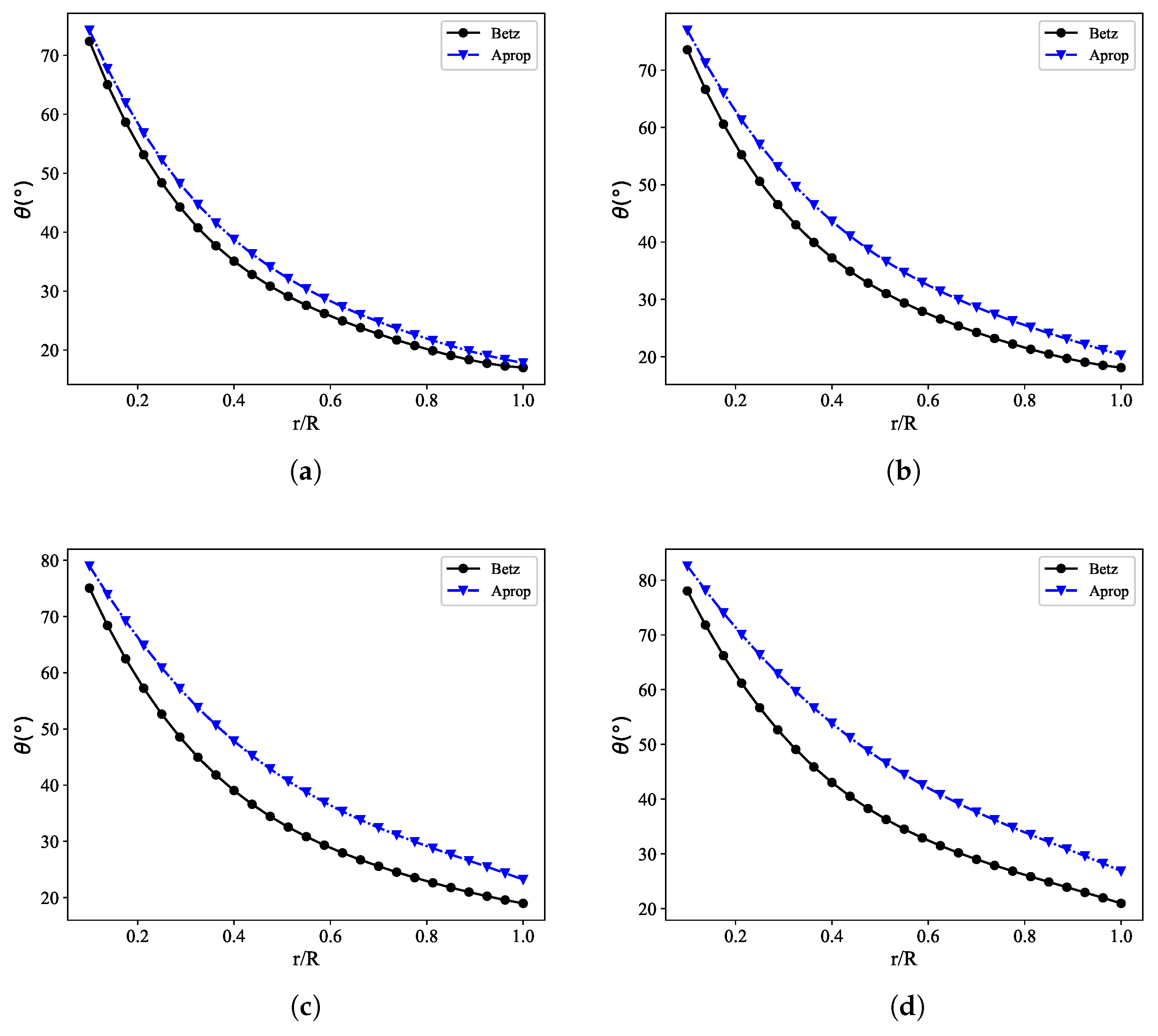
• Calculate the blade pitch angle $\theta$ at each section based on the optimum angle of attack $\alpha$ and inflow angle $\phi$ using Equation (29).
• Determine the airfoil, chord length b, and pitch angle $\theta$ at each section of the propeller by following the above steps, and then determine the geometry of the propeller with a specified number of blades.

The design of the heavy-loaded propeller meeting the specified thrust requirements can be accomplished by simply following the above steps in sequence. In comparison to Adkins’ method [16], which also does not rely on the light loading assumption, this method eliminates the need for iterative execution, hence enabling a rapid completion of the design.

The design method proposed in this paper (hereinafter referred to as Aprop) and that proposed by Adkins are both implemented as computer programs using the Julia language, and the two sets of programs share input-output functions. The aerodynamic performance calculations are conducted using XFOIL. Due to varying Reynolds numbers and Mach numbers for each section, aerodynamic performance calculations for each airfoil are carried out during each iteration. For the four design cases mentioned in Section 3 of this paper, the design method proposed in this paper takes an average of 23.3 s, while the Adkins method converges after an average of 4 iterations, taking an average time of 39.5 s. The time taken by Adkins’ method is 1.70 times that of the Aprop method. Most of the time consumed by both programs is spent performing airfoil performance calculations using XFOIL. Reducing the number of iterations can effectively decrease the overall computation time required. The number of iterations required by the Adkins’ method depends on the initial value of $\zeta$, which is the velocity displacement ratio, and $\zeta =\frac{V^{\prime }}{V_0}$. In this study, the initial value of $\zeta$ is set to 1.0.

The thrust and the torque of the propeller under the design condition can be calculated from Equations (30) and (31), where $dT$ and $dQ$ can be obtained from Equations (10) and (11).

$$T={\int }_{R_h}^{R_t}dT$$

(30)

$$Q={\int }_{R_h}^{R_t}dQ$$

(31)

Under any operating condition, the power of the propeller can be calculated by Equation (32), where Q is the torque, and $\Omega$ is the rotational velocity.

$$P=Q\Omega$$

(32)

The propeller efficiency can be calculated using Equation (33).

$$\eta =\frac{T{V}_0}{P}$$

(33)

3. Results and Discussion

In this section, propellers are designed using these two methods based on the given design conditions, and the blade geometry of the designed propellers is then compared. Later, the aerodynamic performance of the designed propellers, particularly the difference between the actual thrust and the required thrust, is compared using computational fluid dynamics (CFD) analysis.

3.1. Blade Geometry

To verify the effectiveness of the method proposed in this paper, the performance parameters, such as thrust and efficiency of the propeller designed by the method proposed in this paper and the propeller design method based on the Betz condition, are compared under different disc loadings.

The design parameters of the propeller are shown in

Table 1. Propeller design parameter.

${\mathit{V}}_0$	$\mathbf{\Omega }$	${\mathit{R}}_{\mathbf{tip}}$	${\mathit{N}}_{\mathit{b}}$	Airfoil	J
50 m/s	4500 RPM	0.5 m	2	S9000	0.67

, and the standard atmosphere at sea level is adopted. The propeller disc loading is obtained by changing the design thrust.

The blade circulation distribution under different disc loadings is shown in Figure 4. At the root of the blade, the circulation calculated by the design method proposed in this paper is higher—0.9 times larger than the Betz method when the disc loading is 1800 Pa. At the mid-span of the blade, to maintain the same total thrust, the circulation calculated by the Aprop method is smaller than that of the Betz method. Both methods yield the same circulation near the blade tip.

The axial velocity displacement obtained with different design methods is shown in

Table 2. Axial velocity displacement results of different methods.

Disc Load (Pa)	Betz (m/s)	Aprop (m/s)
600	7.38	19.47
1000	12.11	32.85
1400	16.83	46.63
1800	21.57	60.74

. The axial velocity displacement obtained by the Aprop method is larger under any disc loadings. According to Equation (24), the total velocity obtained by the Aprop method is greater when the inflow parameters are the same, and the chord length of the blades at each section obtained by the Aprop method is smaller when the circulation distribution is basically the same. The chord length distribution obtained by the three methods is shown in Figure 5.

Compared to the method based on the Betz condition, the chord length of the blade obtained by the Aprop method is longer at the blade root and tip but shorter in the middle of the blade.

According to Equation (23), the larger the axial velocity displacement, the greater the inflow angle, and the larger the corresponding pitch angle when the angle of attack is the same. The comparison of pitch angle distribution under different disc loadings is shown in Figure 6. Due to the fact that the difference in axial velocity displacement obtained by the three methods increases with the increase of disc loading, the difference in pitch angle also increases with the increase of disc loading.

3.2. Aerodynamic Performance

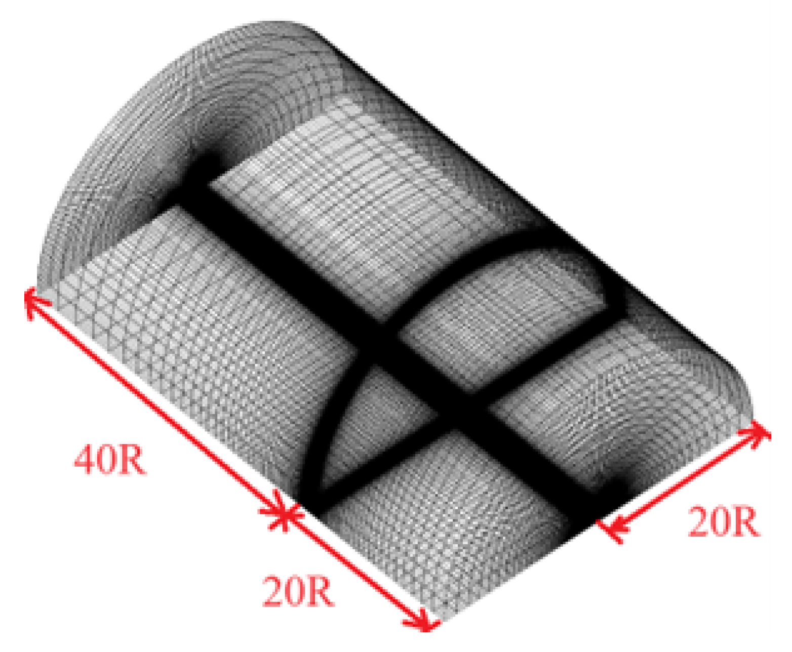
CFD analysis is introduced to validate whether the proposed design method in this paper can generate propellers that meet the tension requirements. Before the CFD analysis, mesh partitioning and mesh independence study were conducted to achieve accurate and reliable results while minimizing computational resources.

Mesh and CFD Setup

The flow around the blade can be considered to be a steady flow for verification of aerodynamic performance with CFD. To reduce the mesh size and improve computational efficiency, periodic mesh is used for the computation, i.e., for the two-blade propeller, only half of the complete mesh is generated, and rotating periodic boundary conditions are used for the computation. The mesh consists of two domains: the rotation domain and the stationary domain. These two domains form an interface via point overlap, thus avoiding errors caused by interpolation of physical quantities on both sides of the interface.

The distance between the mesh inlet and the disc plane is $20R$, the radius of the far-field surface is $20R$, and the distance between the mesh outlet and the disc plane is $40R$, where R is the propeller radius. Mesh topology is shown in Figure 7, and the two domains are shown in Figure 8.

In the rotation domain, a structured grid is adopted for the blade surface (Figure 9), with 111 spanwise grid points and 241 chordwise grid points. Unstructured meshes are adopted for the blade tip and hub. The boundary layer mesh of the blade (Figure 10) is generated using Pointwise’s T-Rex technique(Pointwise V18.0R1) [26] with the height of the first layer being $0.005$ mm, a normal growth rate being 1.2, and a maximum number of layers generated is 40. Unstructured mesh is generated for the rest of the rotation domain.

In the stationary domain, the upstream and downstream of the rotation domain are obtained by stretching the inlet and outlet of the rotation domain, respectively, which are prism meshes. The other parts in the far-field mesh are structured grids.

The flow field is calculated with ANSYS CFX 2020R1 with the multiple reference frames(MRF) model. MRF simulations are sufficient for thrust and torque prediction of an open propeller and can reduce the CPU time of rigid body motion simulations [27]. In the rotation domain, the flow around a propeller by assigning a constant rotational velocity while the solid structure of the propeller itself remains fixed [28,29,30,31].

The mesh size has a significant impact on the CFD results. In general, increasing the mesh size can improve the computation accuracy but also increase the computation time. The mesh independence is studied to balance the computation accuracy and time. The pitch angle at the root of the propeller blade is $63.3°$, at $75\%$ radius, it is $22.5°$, and at the blade tip, the pitch angle is $17.6°$. Without changing the mesh topology, a total of 4 meshes are generated by changing the number of mesh points on different mesh lines, numbered Mesh1 to Mesh4 according to the mesh size. In the four sets of meshes, the minimum mesh size within the rotating domain is 0.00486 mm for all, while the maximum mesh size decreases from 36.175 mm in Mesh1 to 25.462 mm in Mesh4. The minimum grid size within the rotating domain decreases from 4.147 mm in Mesh1 to 1.876 mm in Mesh4, while the maximum mesh size decreases from 2401.5 mm in Mesh1 to 1235.4 mm in Mesh4.

The mesh size and the CFD results of each mesh are shown in

Table 3. CFD results of different meshes.

Mesh	Mesh Size	Thrust (N)	Efficiency (%)
Mesh1	2,115,711	382.08	79.62
Mesh2	3,082,141	381.31	79.63
Mesh3	5,609,432	380.60	79.71
Mesh4	6,025,615	380.23	79.49

. Compared to the results obtained from Mesh4 results, the maximum difference in thrust among the other three meshes is $1.85$ N, which is $0.66\%$ of the thrust from Mesh4, and the maximum difference in efficiency is $0.23\%$, representing $0.29\%$ of the efficiency from Mesh4. The comparison of results indicates that altering the overall mesh quantity has minimal influence on the computed results. Therefore, Mesh2 will be used for the subsequent analysis of propeller performance.

3.3. Comparison of Aerodynamic Performance

The aerodynamic performance of the blade obtained by the different methods in the design state is shown in

Table 4. Propeller performance of different methods.

Disc Load (Pa)	Design Thrust (N)	Design Method	Thrust (N)	Efficiency (%)	Relative Thrust Error (%)
600	471.24	Betz	397.18	78.95	−15.67
		Adkins	408.33	81.19	−13.35
		Aprop	459.63	75.59	−2.42
1000	785.40	Betz	648.94	75.46	−17.33
		Adkins	655.57	77.55	−16.53
		Aprop	797.49	67.97	1.59
1400	1099.56	Betz	875.99	71.97	−20.36
		Adkins	857.34	73.59	−22.03
		Aprop	1069.46	58.39	−2.78
1800	1413.72	Betz	1066.36	68.41	−24.57
		Adkins	1053.84	69.74	−25.46
		Aprop	1318.43	49.12	−6.74

. To study the improvement of the Aprop method relative to the Adkins method, the computational data for the Adkins method is also presented in the table. The designed thrust is calculated based on the disc loading according to Equation (1), and the thrust and efficiency in columns 4 and 5 are the results from CFD analysis. The relative thrust error in Table 4 is defined as

$$te=\frac{T_a-T_r}{T_r}$$

(34)

where $T_a$ is the actual thrust of the propeller, and $T_r$ is the required thrust. The absolute value of the relative thrust error of the propeller designed by the Aprop method is within 5% for disc loading ranging from 600 Pa to 1400 Pa, and is 6.74% for 1800 Pa. The thrust of the propeller was designed based on the Betz condition and the Adkins’ method are below the required thrust. The comparison of relative thrust errors obtained by the three methods is shown in Figure 11.

Figure 12 shows the comparison of propeller thrust coefficient with advance ratio under different disc loadings. The Betz method shows a rapid decrease in the thrust coefficient with an increasing advance ratio under different disc loadings. With a small advance ratio, the thrust coefficient of the propellers designed by the Betz method is greater. After the advance ratio increases, the thrust coefficient of the propeller designed by the Aprop method decreases slowly, and the final thrust coefficient is greater than that designed by the Betz method. As shown in Figure 12, the thrust coefficient of propellers designed by Betz method reduce rapidly with the increase of advance ratio, and its adaptability to wide operating conditions is lower than that of the Aprop method.

The comparison of propeller efficiency under different disc loadings is shown in Figure 13. When the advance ratio is large (for example, greater than 0.9 under a disc loading of 600 Pa), the efficiency of the propeller designed based on the Aprop method is higher than the efficiency of the propeller designed based on the Betz method, and the efficiency difference between these two propellers becomes larger and larger as the advance ratio increases. When the advance ratio is small, the efficiency of the propeller designed based on the Betz method is higher, but the thrust of this propeller does not meet the design requirements. Overall, the maximum efficiency of the propeller designed based on the Aprop method is higher, and the efficiency decline is relatively smooth.

4. Conclusions

Based on the optimal circulation distribution of a finite number of blades, a novel design method applicable to heavy-loaded propellers is proposed, by which the axial velocity displacement is computed via the assumption of constant axial velocity displacement along the radial direction and the relationship between propeller thrust and the axial velocity displacement. In order to verify the design accuracy of this method, the aerodynamic performance of the propeller is analyzed with CFD and then compared to that of the propeller designed based on the Betz condition with the minimum energy loss under the light loading assumption.

The absolute value of the relative thrust error obtained by the design method proposed in this paper is within 5% for disc loading ranging from 600 Pa to 1400 Pa, and is 6.74% for a disc loading of 1800 Pa, indicating little variation with the disc loading. However, the absolute value of the relative thrust error obtained by the design method based on the Betz condition with the minimum energy loss is too large and increases with the increase of the disc loading.

The thrust coefficient of the propeller designed by the method proposed in this paper decreases slowly with the increase of the advance ratio, indicating its good performance under wide working conditions.

Compared to those obtained on the basis of the Betz condition with the minimum energy loss under the light loading assumption, the axial velocity displacement obtained by the design method proposed in this paper is larger, while the circulation distribution is basically the same. Hence, the blade chord length is shorter, and the pitch angle is larger.

After the circulation distribution is obtained by the method based on the Betz condition with the minimum energy loss under the light loading assumption, the thrust can be improved, and efficiency can be kept basically unchanged by amplifying the circulations in equal proportions and increasing the chord length without changing the pitch angle.

References

1. Sinnige, T.; van Arnhem, N.; Stokkermans, T.C.A.; Eitelberg, G.; Veldhuis, L.L.M. Wingtip-Mounted Propellers: Aerodynamic Analysis of Interaction Effects and Comparison with Conventional Layout. J. Aircr. 2018, 56, 295–312. [Google Scholar] [CrossRef]
2. Stoll, A.M.; Bevirt, J.B.; Moore, M.D.; Fredericks, W.J.; Borer, N.K. Drag Reduction Through Distributed Electric Propulsion. In Proceedings of the 14th AIAA Aviation Technology, Integration, and Operations Conference, Atlanta, GA, USA, 16–20 June 2014. [Google Scholar]
3. Firnhaber Beckers, M.; Schollenberger, M.; Lutz, T.; Bongen, D.; Radespiel, R.; Florenciano, J.L.; Funes-Sebastian, D.E. CFD Investigation of High-Lift Propeller Positions for a Distributed Propulsion System. In Proceedings of the AIAA AVIATION 2022 Forum, Chicago, IL, USA, 27 June–1 July 2022. [Google Scholar] [CrossRef]
4. Wu, J.; Gao, F.; Li, S.; Yang, F. Conceptual Design and Optimization of Distributed Electric Propulsion General Aviation Aircraft. Aerospace 2023, 10, 387. [Google Scholar] [CrossRef]
5. Moore, M.D.; Goodrich, K.H. High Speed Mobility through On-Demand Aviation. In Proceedings of the 2013 Aviation Technology, Integration, and Operations Conference, Los Angeles, CA, USA, 12–14 August 2013. [Google Scholar] [CrossRef]
6. Litherland, B.L.; Borer, N.K.; Zawodny, N.S. X-57 Maxwell High-Lift Propeller Testing and Model Development. In Proceedings of the AIAA Aviation 2021 Forum, Virtual Event, 2–6 August 2021. [Google Scholar] [CrossRef]
7. Yoo, S.; Duensing, J.C.; Deere, K.A.; Viken, J.K.; Frederick, M. Computational Analysis on the Effects of High-lift Propellers and Wing-tip Cruise Propellers on X-57. In Proceedings of the AIAA Aviation 2023 Forum, San Diego, CA, USA, 12–16 June 2023; p. 3382. [Google Scholar]
8. Borer, N.K.; Patterson, M.D. X-57 high-lift propeller control schedule development. In Proceedings of the AIAA Aviation 2020 Forum, Online, 15–19 June 2020; p. 3091. [Google Scholar]
9. Huang, Z.; Yao, H.; Lundbladh, A.; Davidson, L. Low-Noise Propeller Design for Quiet Electric Aircraft. In Proceedings of the AIAA Aviation 2020 Forum, Virtual Event, 15–19 June 2020. [Google Scholar] [CrossRef]
10. Keller, D. Towards higher aerodynamic efficiency of propeller-driven aircraft with distributed propulsion. CEAS Aeronaut. J. 2021, 12, 777–791. [Google Scholar] [CrossRef]
11. Rankine, W. On the mechanical principles of the action of propellers. Trans. Inst. Nav. Archit. 1865, 13, 13–30. [Google Scholar]
12. Betz, A. Schraubenpropeller mit geringstem Energieverlust. Mit einem Zusatz von l. Prandtl. Nachrichten Ges. Wiss. Gott. Math.-Phys. Kl. 1919, 1919, 193–217. [Google Scholar]
13. Goldstein, S. On the vortex theory of screw propellers. Proc. R. Soc. London Ser. A Contain. Pap. A Math. Phys. Character 1929, 123, 440–465. [Google Scholar]
14. Theodore, T. Theory of Propellers. Aeronaut. J. 1948, 52, 574. [Google Scholar] [CrossRef]
15. Larrabee, E.E. Practical Design of Minimum Induced Loss Propellers. SAE Trans. 1979, 88, 2053–2062. [Google Scholar]
16. Adkins, C.; Liebeck, R. Design of optimum propellers. In Proceedings of the 21st Aerospace Sciences Meeting, Reno, NV, USA, 10–13 January 1983; American Institute of Aeronautics and Astronautics: Reston, VA, USA, 1983. [Google Scholar] [CrossRef]
17. Traub, L.W. Simplified propeller analysis and design including effects of stall. Aeronaut. J. 2016, 120, 796–818. [Google Scholar] [CrossRef]
18. Patterson, M.D.; Borer, N.K.; German, B. A simple method for high-lift propeller conceptual design. In Proceedings of the 54th AIAA Aerospace Sciences Meeting, San Diego, CA, USA, 4–8 January 2016; p. 0770. [Google Scholar]
19. Patterson, M.D. Conceptual Design of High-Lift Propeller Systems for Small Electric Aircraft. Ph.D. Thesis, Georgia Institute of Technology, Atlanta, GA, USA, 2016. [Google Scholar]
20. Fan, Z.; Zhou, Z.; Zhu, X. A design method for propeller with arbitrary circulation distribution. J. Aerosp. Power 2019, 34, 434–441. [Google Scholar]
21. Wang, K.; Zhou, Z.; Fan, Z.; Guo, J. Aerodynamic design of tractor propeller for high-performance distributed electric propulsion aircraft. Chin. J. Aeronaut. 2021, 34, 20–35. [Google Scholar] [CrossRef]
22. Xue, C.; Zhou, Z. Inverse aerodynamic design for DEP propeller based on desired propeller slipstream. Aerosp. Sci. Technol. 2020, 102, 105820. [Google Scholar] [CrossRef]
23. Young, T.M. International Standard Atmosphere (ISA) Table. In Performance of the Jet Transport Airplane: Analysis Methods, Flight Operations and Regulations; John Wiley & Sons, Ltd.: Chichester, UK, 2017; pp. 583–590. [Google Scholar] [CrossRef]
24. Peng, P.; Yao, L.j. Prediction of Propeller Slipstream Influence Based on Optimal Circulation Distribution. J. Propuls. Technol. 2019, 40, 2692–2699. [Google Scholar] [CrossRef]
25. Drela, M. XFOIL: An Analysis and Design System for Low Reynolds Number Airfoils. In Low Reynolds Number Aerodynamics; Mueller, T.J., Ed.; Springer: Berlin, Heidelberg, 1989; pp. 1–12. [Google Scholar]
26. Cadence. Unstructured Viscous Boundary Layer Meshing: T-Rex. 2023. Available online: https://www.pointwise.com/doc/user-manual/grid/solve/unstructured-blocks/t-rex.html (accessed on 8 October 2023).
27. Bergmann, O.; Götten, F.; Braun, C.; Janser, F. Comparison and evaluation of blade element methods against RANS simulations and test data. CEAS Aeronaut. J. 2022, 13, 535–557. [Google Scholar] [CrossRef]
28. Siddiqi, Z.; Lee, J.W. Experimental and numerical study of novel Coanda-based unmanned aerial vehicle. J. Eng. Appl. Sci. 2022, 69, 1–19. [Google Scholar] [CrossRef]
29. Lopez, O.D.; Escobar, J.A.; Pérez, A.M. Computational Study of the Wake of a Quadcopter Propeller in Hover. In Proceedings of the 23rd AIAA Computational Fluid Dynamics Conference, Denver, CO, USA, 5–9 June 2017. [Google Scholar] [CrossRef]
30. Kutty, H.A.; Rajendran, P. 3D CFD Simulation and Experimental Validation of Small APC Slow Flyer Propeller Blade. Aerospace 2017, 4, 10. [Google Scholar] [CrossRef]
31. Stajuda, M.; Karczewski, M.; Obidowski, D.; Jóźwik, K. Development of a CFD model for propeller simulation. Mech. Mech. Eng. 2016, 20, 579–593. [Google Scholar]
Figure 1. Propeller disc.
Energies 17 00786 g001
Figure 2. Force analysis of blade element under light loading assumption.
Energies 17 00786 g002
Figure 3. Force analysis of heavy-loaded propeller blade element.
Energies 17 00786 g003
Figure 4. Comparison of circulation distribution. (a) Disc loading = 600 Pa. (b) Disc loading = 1000 Pa. (c) Disc loading = 1400 Pa. (d) Disc loading = 1800 Pa.
Energies 17 00786 g004
Figure 5. Comparison of chord distribution. (a) Disc loading = 600 Pa. (b) Disc loading = 1000 Pa. (c) Disc loading = 1400 Pa. (d) Disc loading = 1800 Pa.
Energies 17 00786 g005
Figure 6. Comparison of pitch angle distribution. (a) Disc loading = 600 Pa. (b) Disc loading = 1000 Pa. (c) Disc loading = 1400 Pa. (d) Disc loading = 1800 Pa.
Energies 17 00786 g006
Figure 7. Mesh topology.
Energies 17 00786 g007
Figure 8. Rotational and stationary domain.
Energies 17 00786 g008
Figure 9. Blade surface grid.
Energies 17 00786 g009
Figure 10. Boundary mesh.
Energies 17 00786 g010
Figure 11. Design thrust error of each method.
Energies 17 00786 g011
Figure 12. Comparison of thrust coefficient. (a) Disc loading = 600 Pa. (b) Disc loading = 1000 Pa. (c) Disc loading = 1400 Pa. (d) Disc loading = 1800 Pa.
Energies 17 00786 g012
Figure 13. Comparison of efficiency. (a) Disc loading = 600 Pa. (b) Disc loading = 1000 Pa. (c) Disc loading = 1400 Pa. (d) Disc loading = 1800 Pa.
Energies 17 00786 g013aEnergies 17 00786 g013b