Interval State Estimation of Electricity-Gas Systems Considering Measurement Correlations

Abstract

The popularization of electricity-gas systems leads to increasing demand for state management of systems. However, the existence of neglected measurement correlations brings uncertainties to the electricity-gas systems state estimation. In this paper, an interval state estimation method that considers measurement correlations existing in the electricity-gas systems is presented. We derive the linear measurement model for the electricity-gas systems through Taylor series expansion and estimate the measurement variance-covariance matrix with measurement correlations. The system parameter matrix and the measurement variance-covariance matrix containing measurement correlations are combined into an interval, and the interval state matrix considering measurement correlations is constructed. Then, the linear equations for the state estimation interval considering measurement correlations are established based on the measurement containing correlations and interval state matrix; as a result, the electricity-gas system state estimation model containing measurement correlations is established. In addition, a method for determining the range of state estimation intervals is proposed. Numerical tests on an integrated electricity-gas system comprising a 10-node natural gas network and IEEE 30-bus system indicate that the proposed approach has more advantages over the UT+KO approach in computation accuracy and computation efficiency.

1. Introduction

The popularization of electricity-gas systems leads to increasing demand for system state supervision, and electricity-gas system state estimation is becoming an important role of effective monitoring and control systems [1]. Most studies of state estimation assumed that the measurements follow the independent Gaussian distribution and ignored the correlations of the measurements. Nevertheless, this is not applicable in practice. Since measurement data is usually obtained by the data acquisition system and the same measurement equipment, every step from data acquisition may be affected by the same errors—after the superposition and propagation of these errors, there will be a certain correlation between the measurements [2]. The research shows that the long-term existence of measurement correlations may have adverse effects on the results of electricity-gas systems state estimation [3,4,5], such as the impact on the precision of state estimation in distribution systems [3], as well as the impact of bad data with measurement correlations on the measurement sets [4,5]. Thus, it is necessary to consider the existing measurement correlations in the state estimation of electricity-gas systems. However, in practice, the impact of these correlations on the system is hard to quantify. Therefore, we need to provide the uncertainty range of state variables induced by measurement correlations, and ensure that the state variables always exist in this range, for the sake of reducing the influence of measurement correlations on system safety and ensuring the stability and reliability of energy system.

Currently, there are relatively few studies considering the measurement correlations of the electricity-gas system; most focus on the study of the electricity system, and few involve both the measurement correlation of electricity system and natural gas system. As for the measurement correlations of electricity systems, the unscented transformation (UT) is regarded as an effective solution. For instance, a state estimation framework of electricity system based on UT for measurement correlations and measurements with incomplete time synchronization was developed in [6]. In [7,8,9], UT was employed to calculate the correlations between the measurements of the electricity system and the correlations between the voltage phasor, active and reactive power of the bus. These methods based on UT considered the measurement correlations of electricity systems, obtained the correlation between the measured values through symmetric sampling strategy, and then utilized the covariance to transfer the correlation. Although they had a certain tolerance for measurement correlations, they need to calculate the measurements independently and symmetrically, and are therefore mainly aimed at small-scale electricity systems. As the system size increases, the calculation efficiency will gradually decrease.

In addition to UT, some methods based on the Kalman filter were used to solve measurement correlations, including the Kalman filter (to predict the error covariance matrix) [10,11], and the point estimation method based on an extended Kalman filter [12]. In addition, the combination of untracked transform and Kalman filter has been used to detect bad data with measurement correlations [13]. These Kalman filter methods reduce the measurement correlations by filtering the measurement values, and the state estimation is therefore still based on the filtering and depends on the precise measurement values to a certain extent.

Furthermore, the measured data was modeled as multivariable time series to simulate the spatial correlation in [14,15]. Nevertheless, time series is only suitable for simulating the system state in the short term, and, because it is difficult to accurately describe long-term and fluctuating energy systems, such studies have not delved into the calculation of correlations. Apart from time series, some literatures combined least squares with point estimation to calculate the measurement correlations of electricity systems [16,17,18]. However, least squares is mainly used for linear calculations and is not very suitable for calculating nonlinear relationships in power systems. Although the correlations of load and input variables were considered in other studies, they mainly focus on pseudo-measurements and stochastic power flow calculation [19,20].

The above methods for considering the measurement correlations existing in the state estimation are mainly aimed at the electricity system. Of these methods considering the measurement correlations, the method based on UT obtained the correlation between the measured values through the symmetric sampling strategy, which is inefficient to solve. Although the Kalman filter method reduces the measurement correlation through filtering, the state estimation still depends on the accurate measurement value to a certain extent, and has low tolerance for measurement correlations. The time series is only suitable for simulating short-term system states, and the least squares method is not very suitable for nonlinear energy systems. Individual studies that considered correlation mainly focus on pseudo-measurements and stochastic power flow calculations. Therefore, these existing methods that considered measurement correlations in electricity systems still have some limitations, and current research rarely involves both electricity system and gas system.

To further effectively solve the state estimation of electricity-gas systems considering measurement correlations, an interval state estimation method is developed in this paper. Firstly, we derive the linear measurement model for the electricity-gas systems through Taylor series expansion and estimate the measurement variance-covariance matrix with measurement correlations. Subsequently, we combine the system parameter matrix with the measurement variance-covariance matrix containing measurement correlations into an interval to construct the interval state matrix considering measurement correlations. Then, the linear equations for the state estimation interval considering measurement correlations are established based on the measurement containing correlations and interval state matrix; as a result, the electricity-gas system state estimation model with measurement correlations is constructed. Finally, a method for determining the range of state estimation intervals is presented. By comparing the state estimation interval with the safe operating range of system, we can determine if the safe operating range of the system fully covers the state estimation interval, which helps the system administrators enhance situational awareness capabilities, and guides administrators to make effective adjustments as well as to control the energy system when needed. Compared with stochastic methods, the interval state estimation method does not require iterative calculations, and the obtained interval results are more stable, avoiding the randomness of the results. Nevertheless, stochastic methods rely on random selection and have randomness and uncertainty. For multiple calculations of the same case, the results may differ significantly, making it difficult to ensure the reliability of the obtained results range. An integrated electricity-gas system comprised of the 10-node natural gas network and IEEE 30-bus system is taken for numerical tests, and the estimated results of gas demand, pressure at nodes, voltage amplitude, and voltage angle in the integrated electricity-gas system are validated under different levels of measurement correlation, to attest the effectiveness of the proposed approach.

The main contributions of this paper are summarized as follows:

(1)

The derived linear model for measurements of electricity-gas systems transfers the nonlinear electricity-gas system model into the measurements-based linear model, describing the statistical characteristics of state variables in the nonlinear system through linear equations and converting them into measurements.

(2)

The constructed interval state matrix and the linear equations of state estimation interval consider the correlation between measurements in the electricity-gas system (including the correlation between pressure at node and gas mass flow in the gas network, the correlation between active power and reactive power in the electricity system), and establish the electricity-gas system state estimation model containing these correlations.

(3)

The proposed method for determining the range of state estimation interval allows the existence of measurement correlations, has a certain tolerance for measurement correlations, and provides the ideal distribution range of state variables under various measurement correlations.

The remainder of this paper is organized as follows. Section 2 gives the basic model and the linear measurement model for the electricity-gas systems. Section 3 gives the measurement variance-covariance matrix containing measurement correlations, and also establishes the interval state matrix and linear equations of state estimation interval. Section 4 presents a method for determining the range of state estimation intervals. Section 5 validates the effectiveness of the proposed method on an integrated electricity-gas system. Finally, some conclusions are drawn in Section 6.

2. The Linearized Model for Measuring Electricity-Gas Systems

This part mainly introduces the basic model of electricity-gas system, as well as the linear measurement model for the electricity-gas systems deduced by Taylor series expansion.

2.1. The Gas Pipeline System Model

The transmission of natural gas in a pipe exhibits slow dynamic characteristics, and the influence of temperature on the gas pipeline system can be ignored. It is generally considered that the temperature of natural gas in pipe is close to the ambient temperature, and the driving force of pressure causes natural gas to flow axially along a pipe, as shown in Figure 1.

The dynamic behavior of gas system is depicted via partial differential equations [21,22], and the state variables of natural gas flow mainly include pipeline pressure and gas flow. The dynamic behavior of natural gas system can be expressed as follows:

$$\frac{\mathsf{\partial }\left(\pi \right)}{\mathsf{\partial }t}+\frac{ZRT}{S}\cdot \frac{\mathsf{\partial }\left(\dot{G}\right)}{\mathsf{\partial }L}=0$$

(1a)

$$\frac{\mathsf{\partial }\left(\pi \right)}{\mathsf{\partial }L}+\frac{f\cdot ZRT\cdot \dot{G}\left|\dot{G}\right|}{2d\cdot S^2\cdot \pi }=0$$

(1b)

where $\dot{G}$ denotes the natural gas mass flow, $t$ denotes the time, $t=1,\dots ,N$, $\pi$ refers to the pressure, $Z$ is the gas compressibility factor, $R$ refers to ideal gas constant, $f$ is the friction coefficient, $T$ represents the average temperature of natural gas in the pipeline, $L$ is the pipeline length, $d$ represents the pipe inner diameter, $S$ refers to the pipeline cross-section area.

Since the natural gas system model is a set of partial differential equations, direct calculation is more complex. Therefore, we linearize the above partial differential equations. It is assumed that gas flows unidirectionally in pipelines, so the time step is set as $\mathsf{\Delta }t=T_n/N$, the spatial step is set as $\mathsf{\Delta }L=L/M$, then Equation (1) is rewritten as follows:

$$\frac{\mathsf{\Delta }{\pi }_{i+1}^t-\mathsf{\Delta }{\pi }_{i+1}^{t-1}}{\mathsf{\Delta }t}+\frac{ZRT}{S}\cdot \frac{\mathsf{\Delta }{\dot{G}}_{i+1}^t-\mathsf{\Delta }{\dot{G}}_i^t}{\mathsf{\Delta }L}=0$$

(2a)

$$\frac{\mathsf{\Delta }{\pi }_{i+1}^t-\mathsf{\Delta }{\pi }_i^t}{\mathsf{\Delta }L}+\frac{f\cdot ZRT\cdot {\dot{G}}_{st}}{2d\cdot S^2{\pi }_{st}}\cdot \frac{\mathsf{\Delta }{\dot{G}}_{i+1}^t+\mathsf{\Delta }{\dot{G}}_i^t}{2}=0, t=1,\dots ,N, i=1,\dots ,M-1$$

(2b)

where $\mathsf{\Delta }{\pi }_i^t$ and $\mathsf{\Delta }{\dot{G}}_i^t$ are the pressure and gas flow in the pipe; in length of $i$ at time $t$, $\mathsf{\Delta }{\pi }_{i+1}^t$ denotes the pressure and $\mathsf{\Delta }{\dot{G}}_{i+1}^t$ denotes gas flow in the pipe in length of $i+1$ at time $t$. ${\dot{G}}_{st}$ and ${\pi }_{st}$ represent gas flow and pressure of steady state operation, respectively.

Then, we take a matrix to express the relationship between the gas flow and pressure at the inlet of the pipe and the pressure and gas flow at the pipe outlet, and convert Equation (2) into the matrix form in Equation (3).

$$\left[\begin{array}{l}\mathsf{\Delta }{\pi }_{i+1}^t\\ \mathsf{\Delta }{\dot{G}}_{i+1}^t\end{array}\right]=A_g\left[\begin{array}{l}\frac{\mathsf{\Delta }{\pi }_{i+1}^{t-1}}{\mathsf{\Delta }t}+\frac{ZRT\cdot \mathsf{\Delta }{\dot{G}}_i^t}{S\cdot \mathsf{\Delta }L}\\ \frac{\mathsf{\Delta }{\pi }_i^t}{\mathsf{\Delta }L}-\frac{f\cdot ZRT\cdot {\dot{G}}_{st}\cdot \mathsf{\Delta }{\dot{G}}_i^t}{4d\cdot S^2{\pi }_{st}}\end{array}\right]$$

(3)

where input variables consist of pressure $\mathsf{\Delta }{\pi }_{i+1}^{t-1}$ in the pipe in length of $i+1$ at time $t-1$, gas flow $\mathsf{\Delta }{\dot{G}}_i^t$ in the pipe in length of $i$ at time $t$, pressure $\mathsf{\Delta }{\pi }_i^t$ in the pipeline in length of $i$ at time $t$. The output variables are composed of $\mathsf{\Delta }{\pi }_{i+1}^t$ and $\mathsf{\Delta }{\dot{G}}_{i+1}^t$. $A_g$ denotes network parameter matrix.

For a natural gas network, taking the length of the pipeline as the step, the change of pressure and the mass flow are expressed as:

$$\left[\begin{array}{l}\mathsf{\Delta }{\pi }_j^t\\ \mathsf{\Delta }{\dot{G}}_j^t\end{array}\right]=A_g\left[\begin{array}{l}\frac{\mathsf{\Delta }{\pi }_j^{t-1}}{\mathsf{\Delta }t}+\frac{ZRT\cdot \mathsf{\Delta }{\dot{G}}_i^t}{S\cdot L_{i,j}}\\ \frac{\mathsf{\Delta }{\pi }_i^t}{L_{i,j}}-\frac{f\cdot ZRT\cdot {\dot{G}}_{st}\cdot \mathsf{\Delta }{\dot{G}}_i^t}{4d{S}^2{\pi }_{st}}\end{array}\right] i,j\in \left\{1,\dots ,N_n\right\}$$

(4)

where $N_n$ is the number of node, $L_{i,j}$ is the pipeline length, $\mathsf{\Delta }{\pi }_j^{t-1}$ is the pipeline outlet pressure at node $j$ at time $t-1$, $\mathsf{\Delta }{\pi }_j^t$ is pipeline outlet pressure and $\mathsf{\Delta }{\dot{G}}_j^t$ is outlet gas flow. $\mathsf{\Delta }{\pi }_i^t$ is pipeline inlet pressure and $\mathsf{\Delta }{\dot{G}}_i^t$ is inlet gas flow. The network parameter matrix is expressed as Equation (5). The elements $A_{11}$, $A_{12}$, $A_{21}$, $A_{22}$ of $A$ are represented as below:

$$A_g=\left[\begin{array}{cc}{A}_{11}& A_{12}\\ A_{21}& A_{22}\end{array}\right]$$

(5a)

$$\left\{\begin{array}{l}{A}_{11}=f\cdot {\dot{G}}_{st}\cdot \mathsf{\Delta }t\cdot L_{i,j}^2/A_0\hfill \\ A_{12}=-4d\cdot S\cdot {\pi }_{st}\cdot \mathsf{\Delta }t\cdot L_{i,j}/A_0\hfill \\ A_{21}=-4d\cdot S^2\cdot {\pi }_{st}\cdot \mathsf{\Delta }t\cdot L_{i,j}/\left(ZRT\cdot A_0\right)\hfill \\ A_{22}=4d\cdot S^2\cdot {\pi }_{st}\cdot L_{i,j}^2/\left(ZRT\cdot A_0\right)\hfill \end{array}\right.$$

(5b)

$$A_0=f\cdot {\dot{G}}_{st}{L}_{i,j}^2-4d\cdot S\cdot {\pi }_{st}\cdot \mathsf{\Delta }t$$

(5c)

In a natural gas system, the gas flow at a node should satisfy the mass conservation constraint as:

$${\displaystyle \sum _{i\to }{\dot{G}}_{i,j}}-{\displaystyle \sum _{\to i}{\dot{G}}_{k,i}}+{\dot{G}}_i^{\mathit{load}}-{\dot{G}}_i^{\mathit{inject}}=0$$

(6)

where ${\displaystyle \sum _{i\to }{\dot{G}}_{i,j}}$ is the sum of gas flows from node $i$, ${\displaystyle \sum _{\to i}{\dot{G}}_{k,i}}$ means that the gas flows into $i$ from other nodes, ${\dot{G}}_i^{\mathit{inject}}$ represents the gas injection at node $i$, ${\dot{G}}_i^{\mathit{load}}$ is the gas load at node $i$.

2.2. The Electricity System Model

The electricity system model is represented as follows [23]:

$$P_i=\left(V_i^2-V_i{V}_j\cos {\theta }_{ij}\right)g_{ij}-V_i{V}_j\sin {\theta }_{ij}{b}_{ij}$$

(7)

$$Q_i=-\left(V_i^2-V_i{V}_j\cos {\theta }_{ij}\right)b_{ij}-V_i{V}_j\sin {\theta }_{ij}{g}_{ij}$$

(8)

where $Q_i$ represents the reactive power at bus $i$, $P_i$ denotes the active power at bus $i$, ${\theta }_{ij}$ denotes the voltage angle between bus $i$ and bus $j$, $V_i$ refers to the voltage magnitude at bus $i$, $b_{ij}$ refers to the susceptance, $g_{ij}$ represents the conductance.

In the integrated electricity-gas system, the general efficiency of gas-fired generators in converting natural gas into electric energy is stated as [24]:

$$H_i^g={\alpha }_i^g+{\beta }_i^g\cdot \mathsf{\Delta }{P}_i^g+{\gamma }_i^g{\left(\mathsf{\Delta }{P}_i^g\right)}^2$$

(9)

$$\mathsf{\Delta }{\dot{G}}_i^g=\frac{H_i^g}{GHV}$$

(10)

where $\mathsf{\Delta }{P}_i^g$ represents the electric energy generated by gas-fired generator, $H_i^g$ denotes the heat value of gas, $\mathsf{\Delta }{\dot{G}}_i^g$ represents the gas flow demand, $GHV$ denotes the gross heat value of gas, ${\alpha }_i^g$, ${\beta }_i^g$, and ${\gamma }_i^g$ refer to fuel coefficients.

2.3. The Derivation of Linear Measurement Model for the Electricity-Gas Systems

In this section, we use Taylor series expansion to derive the linear measurement model of electricity-gas systems, thereby further linearizing the nonlinear gas system model, enabling us to then obtain a model for measurement. Firstly, we write the independent variables in the natural gas system, namely, $\mathsf{\Delta }{\pi }_i^t$ and $\mathsf{\Delta }{\dot{G}}_i^t$ at node $i$ in the following function form:

$$\mathsf{\Delta }{\dot{G}}_i^t={\phi }_1^{-1}\left[{\phi }_1\left(\mathsf{\Delta }{\dot{G}}_i^t\right)\right]$$

(11a)

$$\mathsf{\Delta }{\pi }_i^t={\phi }_2^{-1}\left[{\phi }_2\left(\mathsf{\Delta }{\pi }_i^t\right)\right]$$

(11b)

Then, the outlet pressure $\mathsf{\Delta }{\pi }_j^t$ and outlet gas flow $\mathsf{\Delta }{\dot{G}}_j^t$ of the pipeline at node $j$ in Equation (4) are respectively written in the following form:

$$\mathsf{\Delta }{\pi }_j^t=A_{11}\left(\frac{\mathsf{\Delta }{\pi }_j^{t-1}}{\mathsf{\Delta }t}+\frac{ZRT\cdot \mathsf{\Delta }{\dot{G}}_i^t}{S\cdot L_{i,j}}\right)+A_{12}\left(\frac{\mathsf{\Delta }{\pi }_i^t}{L_{i,j}}-\frac{f\cdot ZRT\cdot {\dot{G}}_{st}\cdot \mathsf{\Delta }{\dot{G}}_i^t}{4d{S}^2{\pi }_{st}}\right)$$

(12a)

$$\mathsf{\Delta }{\dot{G}}_j^t=A_{21}\left(\frac{\mathsf{\Delta }{\pi }_j^{t-1}}{\mathsf{\Delta }t}+\frac{ZRT\cdot \mathsf{\Delta }{\dot{G}}_i^t}{S\cdot L_{i,j}}\right)+A_{22}\left(\frac{\mathsf{\Delta }{\pi }_i^t}{L_{i,j}}-\frac{f\cdot ZRT\cdot {\dot{G}}_{st}\cdot \mathsf{\Delta }{\dot{G}}_i^t}{4d{S}^2{\pi }_{st}}\right)$$

(12b)

Subsequently, we linearize $\mathsf{\Delta }{\pi }_j^t$, $\mathsf{\Delta }{\dot{G}}_i^t$, and $\mathsf{\Delta }{\pi }_i^t$ by Taylor series expansion, and obtain:

$${\alpha }_g={\left.\frac{\mathsf{\partial }\mathsf{\Delta }{\pi }_j^t}{\mathsf{\partial }\mathsf{\Delta }{\dot{G}}_i^t}\right|}_{\begin{array}{l}\mathsf{\Delta }{\dot{G}}_i^t=\mathsf{\Delta }{\dot{G}}_{i,0}^t\\ \mathsf{\Delta }{\pi }_i^t=\mathsf{\Delta }{\pi }_{i,0}^t\end{array}}=A_{11}\cdot \frac{ZRT}{S\cdot L_{i,j}}-A_{12}\cdot \frac{f\cdot ZRT\cdot {\dot{G}}_{st}}{4d\cdot S^2\cdot {\pi }_{st}}$$

(13)

$${\beta }_g={\left.\frac{\mathsf{\partial }\mathsf{\Delta }{\pi }_j^t}{\mathsf{\partial }\mathsf{\Delta }{\pi }_i^t}\right|}_{\begin{array}{l}\mathsf{\Delta }{\dot{G}}_i^t=\mathsf{\Delta }{\dot{G}}_{i,0}^t\\ \mathsf{\Delta }{\pi }_i^t=\mathsf{\Delta }{\pi }_{i,0}^t\end{array}}=A_{12}\cdot \frac{1}{L_{i,j}}$$

(14)

$$\mathsf{\Delta }{\dot{G}}_i^t-\mathsf{\Delta }{\dot{G}}_{i,0}^t\approx {\left.\frac{\mathsf{\partial }\mathsf{\Delta }{\dot{G}}_i^t}{\mathsf{\partial }{\phi }_1\left(\mathsf{\Delta }{\dot{G}}_i^t\right)}\right|}_{\mathsf{\Delta }{\dot{G}}_i^t=\mathsf{\Delta }{\dot{G}}_{i,0}^t}\left\{{\phi }_1\left(\mathsf{\Delta }{\dot{G}}_i^t\right)-{\phi }_1\left(\mathsf{\Delta }{\dot{G}}_{i,0}^t\right)\right\}$$

(15)

$$\mathsf{\Delta }{\pi }_i^t-\mathsf{\Delta }{\pi }_{i,0}^t\approx {\left.\frac{\mathsf{\partial }\mathsf{\Delta }{\pi }_i^t}{\mathsf{\partial }{\phi }_2\left(\mathsf{\Delta }{\pi }_i^t\right)}\right|}_{\mathsf{\Delta }{\pi }_i^t=\mathsf{\Delta }{\pi }_{i,0}^t}\left\{{\phi }_2\left(\mathsf{\Delta }{\pi }_i^t\right)-{\phi }_2\left(\mathsf{\Delta }{\pi }_{i,0}^t\right)\right\}$$

(16)

Then, we replace ${\phi }_1\left(\mathsf{\Delta }{\dot{G}}_i^t\right)$ with $\mathsf{\Delta }{\dot{G}}_i^t$ and ${\phi }_2\left(\mathsf{\Delta }{\pi }_i^t\right)$ with $\mathsf{\Delta }{\pi }_i^t$ to obtain the linearized model for measurement $\mathsf{\Delta }{\pi }_j^t$ with respect to variables $\mathsf{\Delta }{\dot{G}}_i^t$ and $\mathsf{\Delta }{\pi }_i^t$:

$$\mathsf{\Delta }{\pi }_j^t\approx {\alpha }_g\left(\mathsf{\Delta }{\dot{G}}_i^t-\mathsf{\Delta }{\dot{G}}_{i,0}^t\right)+{\beta }_g\left(\mathsf{\Delta }{\pi }_i^t-\mathsf{\Delta }{\pi }_{i,0}^t\right)+\mathsf{\Delta }{\pi }_{j,0}^t$$

(17)

where, we take ${\dot{G}}_{st}$ and ${\pi }_{st}$ in steady state as the initial values, expressed as $\mathsf{\Delta }{\pi }_{i,0}^t$ and $\mathsf{\Delta }{\dot{G}}_{i,0}^t$, respectively. $\mathsf{\Delta }{\pi }_{j,0}^t$ can be derived from Equations (12a), (13)–(15).

For the electricity system, the voltage amplitude $V$ and voltage angle ${\theta }_{ij}$ are represented in the following function form:

$$V={\varphi }_1^{-1}\left[{\varphi }_1\left(V\right)\right]$$

(18a)

$${\theta }_{ij}={\varphi }_2^{-1}\left[{\varphi }_2\left({\theta }_{ij}\right)\right]$$

(18b)

Then, we linearize the active power $P_i$ injected at bus $i$ via Taylor series expansion to obtain the linearized model for measurement $P_i$, with respect to voltage amplitude $V$ and voltage angle ${\theta }_{ij}$:

$$\begin{array}{l}{P}_i-P_{i,0}\approx {\left.\frac{\mathsf{\partial }{P}_i}{\mathsf{\partial }{V}_i{V}_j}\right|}_{\begin{array}{l}V=V_0\\ {\theta }_{i,j}={\theta }_{ij,0}\end{array}}\left(V_i{V}_j-V_{i,0}{V}_{j,0}\right)+{\left.\frac{\mathsf{\partial }{P}_i}{\mathsf{\partial }{\theta }_{ij}}\right|}_{\begin{array}{l}V=V_0\\ {\theta }_{i,j}={\theta }_{ij,0}\end{array}}\left({\theta }_{ij}-{\theta }_{ij,0}\right)\\ ={\left.\frac{\mathsf{\partial }{P}_i}{\mathsf{\partial }{V}_i{V}_j}\right|}_{\begin{array}{l}V=V_0\\ {\theta }_{i,j}={\theta }_{ij,0}\end{array}}\left\{{\left.\frac{\mathsf{\partial }{V}_i{V}_j}{\mathsf{\partial }{\varphi }_1\left(V_i\right)}\right|}_{V=V_0}\left\{{\varphi }_1\left(V_i\right)-{\varphi }_1\left(V_{i,0}\right)\right\}+{\left.\frac{\mathsf{\partial }{V}_i{V}_j}{\mathsf{\partial }{\varphi }_1\left(V_j\right)}\right|}_{V=V_0}\left\{{\varphi }_1\left(V_j\right)-{\varphi }_1\left(V_{j,0}\right)\right\}\right\}\\ +{\left.\frac{\mathsf{\partial }{P}_i}{\mathsf{\partial }{\theta }_{ij}}\right|}_{\begin{array}{l}V=V_0\\ {\theta }_{i,j}={\theta }_{ij,0}\end{array}}\left\{{\left.\frac{\mathsf{\partial }{\theta }_{ij}}{\mathsf{\partial }{\varphi }_2\left({\theta }_{ij}\right)}\right|}_{{\theta }_{ij}={\theta }_{ij,0}}\left\{{\varphi }_2\left({\theta }_{ij}\right)-{\varphi }_2\left({\theta }_{ij,0}\right)\right\}\right\}\end{array}$$

(19)

where we take voltage amplitude, as well as voltage angle at the balance node in electricity systems, as the initial values, denoted as $V_{i,0}$, $V_{j,0}$, and ${\theta }_{ij,0}$.

We define ${\alpha }_e$ and ${\beta }_e$ as:

$${\left.{\alpha }_e=\frac{\mathsf{\partial }{P}_i}{\mathsf{\partial }{V}_i{V}_j}\right|}_{\begin{array}{l}V=V_0\\ {\theta }_{i,j}={\theta }_{ij,0}\end{array}}$$

(20a)

$${\beta }_e={\left.\frac{\mathsf{\partial }{P}_i}{\mathsf{\partial }{\theta }_{ij}}\right|}_{\begin{array}{l}V=V_0\\ {\theta }_{i,j}={\theta }_{ij,0}\end{array}}$$

(20b)

Assuming that there is only one branch connection between bus $i$ and bus $j$, we replace ${\varphi }_1\left(V\right)$ with $V$ and ${\varphi }_2\left({\theta }_{ij}\right)$ with ${\theta }_{ij}$ to obtain a linearized model for measurement $P_i$ with respect to voltage amplitude $V$ and voltage angle ${\theta }_{ij}$:

$$P_i\approx {\alpha }_e\left(V_i{V}_j-V_{i,0}{V}_{j,0}\right)+{\beta }_e\left({\theta }_{ij}-{\theta }_{ij,0}\right)+P_{i,0}$$

(21)

It should be noted that Equations (19)–(21) represent the case where there is only one branch between bus $i$ and bus $j$. For other special cases with multiple branches, the flux increment needs to be summed.

3. The Construction of State Matrix and Linear Equations of State Estimation Interval Considering Measurement Correlations

In this section, we calculate the measurement variance-covariance matrix containing measurement correlations, and combine the system parameter matrix and measurement variance-covariance matrix into a unified framework to construct a state matrix considering measurement correlations, and construct the state estimation model of the electricity-gas systems containing measurement correlations.

3.1. The Calculation of Measurement Variance-Covariance Matrix with Measurement Correlations

We extend the gas flow $\mathsf{\Delta }{\dot{G}}_i^t$ and pressure $\mathsf{\Delta }{\pi }_i^t$ at pipeline inlet of the natural gas network to $\mathsf{\Delta }{\pi }_{i,k}^t$ and $\mathsf{\Delta }{\dot{G}}_{i,k}^t$ with the same mean and variance, as follows:

$$\mathsf{\Delta }{\pi }_{i,k}^t=\left\{\begin{array}{l}\mathsf{\Delta }{\overline{\pi }}_i^t+{\delta }_{\mathsf{\Delta }{\pi }_i^t}, if k=1\\ \mathsf{\Delta }{\overline{\pi }}_i^t-{\delta }_{\mathsf{\Delta }{\pi }_i^t}, if k=2\end{array}\right.$$

(22)

$$\mathsf{\Delta }{\dot{G}}_{i,k}^t=\left\{\begin{array}{l}\mathsf{\Delta }{\overline{\dot{G}}}_i^t+{\delta }_{\mathsf{\Delta }{\dot{G}}_i^t}, if k=1\\ \mathsf{\Delta }{\overline{\dot{G}}}_i^t-{\delta }_{\mathsf{\Delta }{\dot{G}}_i^t}, if k=2\end{array}\right.$$

(23)

where $\mathsf{\Delta }{\overline{\pi }}_i^t$ and $\mathsf{\Delta }{\overline{\dot{G}}}_i^t$ are the means of $\mathsf{\Delta }{\pi }_i^t$ and $\mathsf{\Delta }{\dot{G}}_i^t$, respectively, and ${\delta }_{\mathsf{\Delta }{\pi }_i^t}$ and ${\delta }_{\mathsf{\Delta }{\dot{G}}_i^t}$ are the standard deviations of $\mathsf{\Delta }{\pi }_i^t$ and $\mathsf{\Delta }{\dot{G}}_i^t$, respectively.

Then, we replace $\mathsf{\Delta }{\dot{G}}_i^t$ with $\mathsf{\Delta }{\dot{G}}_{i,k}^t$ and $\mathsf{\Delta }{\pi }_i^t$ with $\mathsf{\Delta }{\pi }_{i,k}^t$, and rewrite (15) as:

$$\mathsf{\Delta }{\pi }_{j,k}^t={\alpha }_g\left(\mathsf{\Delta }{\dot{G}}_{i,k}^t-\mathsf{\Delta }{\dot{G}}_{i,0}^t\right)+{\beta }_g\left(\mathsf{\Delta }{\pi }_{i,k}^t-\mathsf{\Delta }{\pi }_{i,0}^t\right)+\mathsf{\Delta }{\pi }_{j,0}^t$$

(24)

where $\mathsf{\Delta }{\pi }_{j,k}^t=\left\{\mathsf{\Delta }{\pi }_{j,1}^t,\mathsf{\Delta }{\pi }_{j,2}^t\right\}$; similarly, we also need to calculate the expanded $\mathsf{\Delta }{\dot{G}}_{j,k}^t$, and finally obtain $\mathsf{\Delta }{\dot{G}}_{j,k}^t=\left\{\mathsf{\Delta }{\dot{G}}_{j,1}^t,\mathsf{\Delta }{\dot{G}}_{j,2}^t\right\}$.

We select $N$ sets of experimental data and calculate the measurement variance-covariance matrix on the basis of an extended matrix:

$$\mathsf{\Delta }{\overline{\pi }}_j^t=E\left[\mathsf{\Delta }{\pi }_{j,k}^t\right]=\frac{1}{2N}{\displaystyle \sum _{n=1}^N{\displaystyle \sum _{k=1}^2\mathsf{\Delta }{\pi }_{j,k}^{t,\left(n\right)}}}$$

(25)

$$\mathsf{\Delta }{\overline{\dot{G}}}_j^t=E\left[\mathsf{\Delta }{\dot{G}}_{j,k}^t\right]=\frac{1}{2N}{\displaystyle \sum _{n=1}^N{\displaystyle \sum _{k=1}^2\mathsf{\Delta }{\dot{G}}_{j,k}^{t,\left(n\right)}}}$$

(26)

$${\sigma }_{\mathsf{\Delta }{\pi }_j^t}^2=\frac{1}{2N}{\displaystyle \sum _{n=1}^N{\displaystyle \sum _{k=1}^2\left[\left(\mathsf{\Delta }{\pi }_{j,k}^{t,\left(n\right)}-\mathsf{\Delta }{\overline{\pi }}_j^t\right){\left(\mathsf{\Delta }{\pi }_{j,k}^{t,\left(n\right)}-\mathsf{\Delta }{\overline{\pi }}_j^t\right)}^{{\rm T}}\right]}}$$

(27)

$${\sigma }_{\mathsf{\Delta }{\dot{G}}_j^t}^2=\frac{1}{2N}{\displaystyle \sum _{n=1}^N{\displaystyle \sum _{k=1}^2\left[\left(\mathsf{\Delta }{\dot{G}}_{j,k}^{t,\left(n\right)}-\mathsf{\Delta }{\overline{\dot{G}}}_{j,k}^t\right){\left(\mathsf{\Delta }{\dot{G}}_{j,k}^{t,\left(n\right)}-\mathsf{\Delta }{\overline{\dot{G}}}_{j,k}^t\right)}^{{\rm T}}\right]}}$$

(28)

where $\mathsf{\Delta }{\overline{\pi }}_j^t$ and $\mathsf{\Delta }{\overline{\dot{G}}}_j^t$ are the mean values of pressure and gas flow, respectively. ${\sigma }_{\mathsf{\Delta }{\pi }_j^t}^2$, ${\sigma }_{\mathsf{\Delta }{\dot{G}}_j^t}^2$ are variances of pressure and gas flow, respectively.

We further calculate the correlation parameters of gas network measurements. For the measurement variance-covariance matrix, the non-diagonal term corresponds to the value of the measurement correlations. We take the product of standard deviation of the measurements and the correlation coefficient between the measurements as measurement correlation parameters, as follows:

$${\mathit{Corr}}_{\mathsf{\Delta }{\pi }_j^t,\mathsf{\Delta }{\dot{G}}_j^t}={\sigma }_{\mathsf{\Delta }{\pi }_j^t}\cdot {\sigma }_{\mathsf{\Delta }{\dot{G}}_j^t}\cdot {\rho }_{\mathsf{\Delta }{\pi }_j^t,\mathsf{\Delta }{\dot{G}}_j^t}$$

(29)

$${\sum }_g=\left[\begin{array}{cc}{\sigma }_{\mathsf{\Delta }{\pi }_j^t}^2& {\mathit{Corr}}_{\mathsf{\Delta }{\pi }_j^t,\mathsf{\Delta }{\dot{G}}_j^t}\\ {\mathit{Corr}}_{\mathsf{\Delta }{\dot{G}}_j^t,\mathsf{\Delta }{\pi }_j^t}& {\sigma }_{\mathsf{\Delta }{\dot{G}}_j^t}^2\end{array}\right]$$

(30)

where ${\sigma }_{\mathsf{\Delta }{\pi }_j^t}$ is the standard deviation of $\mathsf{\Delta }{\pi }_j^t$, ${\sigma }_{\mathsf{\Delta }{\dot{G}}_j^t}$ is standard deviation of the outlet gas flow $\mathsf{\Delta }{\dot{G}}_j^t$, ${\rho }_{\mathsf{\Delta }{\pi }_j^t,\mathsf{\Delta }{\dot{G}}_j^t}$ is the correlation coefficient between the measurement $\mathsf{\Delta }{\pi }_j^t$ and $\mathsf{\Delta }{\dot{G}}_j^t$, ${\sum }_g$ is the measurement variance-covariance matrix in the gas system considering the measurement correlations.

Similar to the gas system, we extend voltage amplitude $V$ as well as voltage angle ${\theta }_{ij}$ in the electricity system to $V_{i,k}$, $V_{j,k}$, ${\theta }_{ij,k}$ with the same mean and variance, as follows:

$$V_{i,k}=\left\{\begin{array}{l}{\overline{V}}_i+{\delta }_{V_i}, if k=1\\ {\overline{V}}_i-{\delta }_{V_i}, if k=2\end{array}\right.$$

(31)

$$V_{j,k}=\left\{\begin{array}{l}{\overline{V}}_j+{\delta }_{V_j}, if k=1\\ {\overline{V}}_j-{\delta }_{V_j}, if k=2\end{array}\right.$$

(32)

$${\theta }_{ij,k}=\left\{\begin{array}{l}{\overline{\theta }}_{ij}+{\delta }_{{\theta }_{ij}}, if k=1\\ {\overline{\theta }}_{ij}-{\delta }_{{\theta }_{ij}}, if k=2\end{array}\right.$$

(33)

Furthermore, we assume that there is only one branch connection between bus $i$ and bus $j$; we replace $V_i$ with $V_{i,k}$, $V_j$ with $V_{j,k}$, and ${\theta }_{ij}$ with ${\theta }_{ij,k}$, and Equation (21) is rewritten as:

$$P_{i,k}={\alpha }_e\left(V_{i,k}{V}_{j,k}-V_{i,0}{V}_{j,0}\right)+{\beta }_e\left({\theta }_{ij,k}-{\theta }_{ij,0}\right)+P_{i,0}$$

(34)

where $P_{i,k}=\left\{P_{i,1},P_{i,2}\right\}$, Equation (34) represents the case where there is only one branch between bus $i$ and bus $j$; for other special cases where there are multiple branches, the flux increment needs to be summed. Similarly, we also need to calculate the expanded $Q_{i,k}$, and finally obtain $Q_{i,k}=\left\{Q_{i,1},Q_{i,2}\right\}$.

We calculate a measurement variance-covariance matrix of the electricity system as follows:

$${\overline{P}}_i=E\left[P_{i,k}\right]=\frac{1}{2N}{\displaystyle \sum _{n=1}^N{\displaystyle \sum _{k=1}^2{P}_{i,k}^{\left(n\right)}}}$$

(35)

$${\overline{Q}}_i=E\left[Q_{i,k}\right]=\frac{1}{2N}{\displaystyle \sum _{n=1}^N{\displaystyle \sum _{k=1}^2{Q}_{i,k}^{\left(n\right)}}}$$

(36)

$${\sigma }_{P_i}^2=\frac{1}{2N}{\displaystyle \sum _{n=1}^N{\displaystyle \sum _{k=1}^2\left[\left(P_{i,k}^{\left(n\right)}-\overline{P}\right){\left(P_{i,k}^{\left(n\right)}-{\overline{P}}_i\right)}^{{\rm T}}\right]}}$$

(37)

$${\sigma }_{Q_i}^2=\frac{1}{2N}{\displaystyle \sum _{n=1}^N{\displaystyle \sum _{k=1}^2\left[\left(Q_{i,k}^{\left(n\right)}-{\overline{Q}}_i\right){\left(Q_{i,k}^{\left(n\right)}-{\overline{Q}}_i\right)}^{{\rm T}}\right]}}$$

(38)

where ${\overline{P}}_i$ denotes mean value of active power and ${\overline{Q}}_i$ denotes mean value of reactive power, respectively; ${\sigma }_{P_i}^2$ is variance of active power, ${\sigma }_{Q_i}^2$ is variance of reactive power.

We then calculate measurement correlation parameters of electricity systems. For the electricity system measurement variance-covariance matrix, we take the product of standard deviation of measurement and correlation coefficient between measurements as the measurement correlation parameter, which is expressed as a non-diagonal term, as shown below:

$${\mathit{Corr}}_{P_i,Q_i}={\sigma }_{P_i}\cdot {\sigma }_{Q_i}\cdot {\rho }_{P_i,Q_i}$$

(39)

$${\sum }_e=\left[\begin{array}{cc}{\sigma }_{P_i}^2& {\mathit{Corr}}_{P_i,Q_i}\\ {\mathit{Corr}}_{Q_i,P_i}& {\sigma }_{Q_i}^2\end{array}\right]$$

(40)

where ${\sigma }_{P_i}$ is standard deviation of active power, ${\sigma }_{Q_i}$ is standard deviation of reactive power, ${\rho }_{P_i,Q_i}$ represents the correlation coefficient between measurements $P_i$ and $Q_i$, and ${\sum }_e$ represent the measurement variance-covariance matrix considering measurement correlations in electricity systems.

3.2. Constructing the State Matrix and Linear Equations of State Estimation Interval Considering Measurement Correlations

Considering the existence of measurement correlations, we combine the natural gas network parameter matrix $A_g$ in Equation (5) with the measurement variance-covariance matrix ${\sum }_g$ in Equation (30) into a framework through interval to further construct the state matrix ${\tilde{A}}_g$ considering the measurement correlations of natural gas network.

Firstly, we extend the natural gas network parameter matrix $A_g$ in Equation (5), as follows:

$$A_g^{*}=\left[\begin{array}{cc}{A}_g& \left(\begin{array}{cc}1& 0\\ 0& 1\end{array}\right)\\ \left(\begin{array}{cc}0& 0\\ 0& 0\end{array}\right)& \left(\begin{array}{cc}1& 0\\ 0& 1\end{array}\right)\end{array}\right]$$

(41)

where $A_g^{*}$ is the expanded natural gas network parameter matrix.

We represent the natural gas network state variables $\mathsf{\Delta }{\pi }_i^t$ and $\mathsf{\Delta }{\dot{G}}_i^t$ in Equation (4) as $X_g$, and include the measurement noise $e_{\mathsf{\Delta }{\pi }_j^t}$ and $e_{\mathsf{\Delta }{\dot{G}}_j^t}$ in $X_g$, as follows:

$$X_g=\left[\begin{array}{c}\frac{\mathsf{\Delta }{\pi }_{i+1}^{t-1}}{\mathsf{\Delta }t}+\frac{ZRT\cdot \mathsf{\Delta }{\dot{G}}_i^t}{S\cdot \mathsf{\Delta }L}\\ \frac{\mathsf{\Delta }{\pi }_i^t}{\mathsf{\Delta }L}-\frac{f\cdot ZRT\cdot {\dot{G}}_{st}\cdot \mathsf{\Delta }{\dot{G}}_i^t}{4d{S}^2{\pi }_{st}}\\ e_{\mathsf{\Delta }{\pi }_j^t}\\ e_{\mathsf{\Delta }{\dot{G}}_j^t}\end{array}\right]$$

(42)

where $e_{\mathsf{\Delta }{\pi }_j^t}$ and $e_{\mathsf{\Delta }{\dot{G}}_j^t}$ take the standard deviation of measurements $\mathsf{\Delta }{\pi }_j^t$ and $\mathsf{\Delta }{\dot{G}}_j^t$.

Then, we use $B_g^{*}$ to denote the measurements $\mathsf{\Delta }{\pi }_j^t$ and $\mathsf{\Delta }{\dot{G}}_j^t$, and extend the matrix as follows:

$$B_g^{*}=\left[\begin{array}{c}\mathsf{\Delta }{\pi }_j^t\\ \mathsf{\Delta }{\dot{G}}_j^t\\ e_{\mathsf{\Delta }{\pi }_j^t}\\ e_{\mathsf{\Delta }{\dot{G}}_j^t}\end{array}\right]$$

(43)

The relationship between extended gas network parameter matrix $A_g^{*}$, natural gas network state variable $X_g$, and measurement $B_g^{*}$ is established as follows:

$$\left[\begin{array}{cc}{A}_g& \left(\begin{array}{cc}1& 0\\ 0& 1\end{array}\right)\\ \left(\begin{array}{cc}0& 0\\ 0& 0\end{array}\right)& \left(\begin{array}{cc}1& 0\\ 0& 1\end{array}\right)\end{array}\right]\left[\begin{array}{c}\frac{\mathsf{\Delta }{\pi }_{i+1}^{t-1}}{\mathsf{\Delta }t}+\frac{ZRT\cdot \mathsf{\Delta }{\dot{G}}_i^t}{S\cdot \mathsf{\Delta }L}\\ \frac{\mathsf{\Delta }{\pi }_i^t}{\mathsf{\Delta }L}-\frac{f\cdot ZRT\cdot {\dot{G}}_{st}\cdot \mathsf{\Delta }{\dot{G}}_i^t}{4d{S}^2{\pi }_{st}}\\ e_{\mathsf{\Delta }{\pi }_j^t}\\ e_{\mathsf{\Delta }{\dot{G}}_j^t}\end{array}\right]=\left[\begin{array}{c}\mathsf{\Delta }{\pi }_j^t\\ \mathsf{\Delta }{\dot{G}}_j^t\\ e_{\mathsf{\Delta }{\pi }_j^t}\\ e_{\mathsf{\Delta }{\dot{G}}_j^t}\end{array}\right]$$

(44)

According to Equations (41)–(43), Equation (44) is further rewritten as:

$$A_g^{*}{X}_g=B_g^{*}$$

(45)

Furthermore, considering the computational dimension of the matrix and taking ${\sum }_g^{-1}\cdot \left[e_{\mathsf{\Delta }{\pi }_j^t};e_{\mathsf{\Delta }{\dot{G}}_j^t}\right]=\left[0;0\right]$ as the target for calculation, we extend the measurement variance-covariance matrix ${\sum }_g$ considering measurement correlations in Equation (30) as follows:

$${\delta }_g=\left[\begin{array}{cc}\left(\begin{array}{cc}1& 0\\ 0& 1\end{array}\right)& \left(\begin{array}{cc}1& 0\\ 0& 1\end{array}\right)\\ \left(\begin{array}{cc}0& 0\\ 0& 0\end{array}\right)& {\sum }_g^{-1}\end{array}\right]$$

(46)

where ${\delta }_g$ is the extended matrix with respect to ${\sum }_g$.

We take $s=\left[s_1,s_2,\dots ,s_n\right]$ to represent correlation factor, and $s_i\in \left\{\left.s_i\in ℝ\right|-1\le s_i\le 1\right\}$, $i=1,2,\dots ,n$. We combine expanded matrix $A_g^{*}$ and expanded measurement variance-covariance matrix ${\delta }_g$ considering measurement correlation into the interval, as follows:

$${\tilde{A}}_g=A_g^{*}+s{\delta }_g, {\tilde{A}}_g\in \left[{\tilde{A}}_g^{*}-{\delta }_g,{\tilde{A}}_g^{*}+{\delta }_g\right]$$

(47)

where ${\tilde{A}}_g$ denotes the natural gas system state matrix with measurement correlation.

We represent ${\tilde{A}}_g$ in Equation (47) as the interval $\left[{\tilde{A}}_g\right]$, where ${\tilde{A}}_g\in \left[{\underset{\_}{\tilde{A}}}_g,{\overline{\tilde{A}}}_g\right]$, we define $\left[{\tilde{A}}_g\right]$ as:

$$\left[{\tilde{A}}_g\right]=\left[{\underset{\_}{\tilde{A}}}_g,{\overline{\tilde{A}}}_g\right]=\left\{\left.{\tilde{A}}_g\in ℝ\right|{\underset{\_}{\tilde{A}}}_g\le {\tilde{A}}_g\le {\overline{\tilde{A}}}_g\right\}$$

(48)

where ${\underset{\_}{\tilde{A}}}_g$ is lower bound of interval $\left[{\tilde{A}}_g\right]$, ${\overline{\tilde{A}}}_g$ is upper bound of interval $\left[{\tilde{A}}_g\right]$.

Similarly, we rewrite the measurements $B_g^{*}$ containing the correlations of natural gas network measurements as interval $\left[B_g\right]$ and introduce $\mathsf{\Delta }{B}_g$ as follows:

$$B_g=B_g^{*}+s\mathsf{\Delta }{B}_g, B_g\in \left[B_g^{*}-\mathsf{\Delta }{B}_g,B_g^{*}+\mathsf{\Delta }{B}_g\right]$$

(49)

$$\mathsf{\Delta }{B}_g=\left[\begin{array}{c}{e}_{\mathsf{\Delta }{\pi }_j^t}\\ e_{\mathsf{\Delta }{\dot{G}}_j^t}\\ 0\\ 0\end{array}\right]$$

(50)

where $e_{\mathsf{\Delta }{\pi }_j^t}$ and $e_{\mathsf{\Delta }{\dot{G}}_j^t}$ take standard deviation of $\mathsf{\Delta }{\pi }_j^t$, $\mathsf{\Delta }{\dot{G}}_j^t$, respectively.

Then, the $X_g$ of the natural gas network is represented as interval $\left[X_g\right]$. Based on Equations (45)–(50), combined with Equations (45), (47) and (49), we can obtain the approximate linear equation of state estimation interval that considers measurement correlations of the natural gas network.

$$\left[A_g^{*}+s{\delta }_g\right]\left[X_g\right]\approx \left[B_g^{*}+s\mathsf{\Delta }{B}_g\right]$$

(51)

For electricity systems, the transformation of system model into equation form is given by [25]; active power $P_i$, reactive power $Q_i$, voltage amplitude $V$, and voltage angle $\theta$ are classified according to different bus types:

$$\left[\begin{array}{c}{P}_L\\ P_S\\ P_R\\ Q_L\\ Q_S\\ Q_R\end{array}\right]=\left[\begin{array}{cccccc}{A}_{11}& A_{12}& A_{13}& A_{14}& A_{15}& A_{16}\\ A_{21}& A_{22}& A_{23}& A_{24}& A_{25}& A_{26}\\ A_{31}& A_{32}& A_{33}& A_{34}& A_{35}& A_{36}\\ A_{41}& A_{42}& A_{43}& A_{44}& A_{45}& A_{46}\\ A_{51}& A_{52}& A_{53}& A_{54}& A_{55}& A_{56}\\ A_{61}& A_{62}& A_{63}& A_{64}& A_{65}& A_{66}\end{array}\right]\left[\begin{array}{c}{\theta }_L\\ {\theta }_S\\ {\theta }_R\\ V_L\\ V_S\\ V_R\end{array}\right]+\left[\begin{array}{c}{C}_1\\ C_2\\ C_3\\ C_4\\ C_5\\ C_6\end{array}\right]$$

(52)

$$\left\{\begin{array}{l}P={\left[\begin{array}{ccc}{P}_L^T& P_S^T& P_R^T\end{array}\right]}^T\\ Q={\left[\begin{array}{ccc}{Q}_L^T& Q_S^T& Q_R^T\end{array}\right]}^T\\ V={\left[\begin{array}{ccc}{V}_L^T& V_S^T& V_R^T\end{array}\right]}^T\\ \theta ={\left[\begin{array}{ccc}{\theta }_L^T& {\theta }_S^T& {\theta }_R^T\end{array}\right]}^T\end{array}\right.$$

(53)

where subscript $L$ denotes $PQ$ bus, subscript $S$ denotes $PV$ bus, subscript $R$ denotes $V\theta$ bus. $A_{ij}$ is the electricity system parameter matrix, $C_i$ is the constant term.

Considering the electricity system measurement correlations, the parameter matrix $A_{ij}$ is represented as $A_e$ and it is extended as:

$$A_e^{*}=\left[\begin{array}{cc}{A}_e& \left(\begin{array}{cc}1& 0\\ 0& 1\end{array}\right)\\ \left(\begin{array}{cc}0& 0\\ 0& 0\end{array}\right)& \left(\begin{array}{cc}1& 0\\ 0& 1\end{array}\right)\end{array}\right]$$

(54)

where $A_e^{*}$ refers to the expanded electricity system parameter matrix.

The $X_e$ is employed to represent the $V$ and $\theta$ of electricity system in Equation (52), and measurement noise $e_{P_i}$ and $e_{Q_i}$ are included as follows:

$$X_e=\left[\begin{array}{c}\theta \\ V\\ e_{P_i}\\ e_{Q_i}\end{array}\right]$$

(55)

where $e_{P_i}$ and $e_{Q_i}$ take the standard deviation of $P$ and $Q$, respectively.

Then, we use $B_e^{*}$ to represent the measurements $P$ and $Q$ in the electricity system, and extend the matrix as follows:

$$B_e^{*}=\left[\begin{array}{c}P\\ Q\\ e_{P_i}\\ e_{Q_i}\end{array}\right]$$

(56)

The relationship between the extended electricity system parameter matrix $A_e^{*}$, electricity system state variables $X_e$, and measurement $B_e^{*}$ is established as follows:

$$\left[\begin{array}{cc}{A}_e& \left(\begin{array}{cc}1& 0\\ 0& 1\end{array}\right)\\ \left(\begin{array}{cc}0& 0\\ 0& 0\end{array}\right)& \left(\begin{array}{cc}1& 0\\ 0& 1\end{array}\right)\end{array}\right]\left[\begin{array}{c}\theta \\ V\\ e_{P_i}\\ e_{Q_i}\end{array}\right]=\left[\begin{array}{c}P\\ Q\\ e_{P_i}\\ e_{Q_i}\end{array}\right]$$

(57)

We denote Equation (57) as:

$$A_e^{*}{X}_e=B_e^{*}$$

(58)

Then, considering the computational dimension of the matrix and taking ${\sum }_e^{-1}\cdot \left[e_{P_i};e_{Q_i}\right]=\left[0;0\right]$ as the target for calculation, we extend the measurement variance-covariance matrix ${\sum }_e$ considering measurement correlations in Equation (40) as follows:

$${\delta }_e=\left[\begin{array}{cc}\left(\begin{array}{cc}1& 0\\ 0& 1\end{array}\right)& \left(\begin{array}{cc}1& 0\\ 0& 1\end{array}\right)\\ \left(\begin{array}{cc}0& 0\\ 0& 0\end{array}\right)& {\sum }_e^{-1}\end{array}\right]$$

(59)

where ${\delta }_e$ is the expanded measurement variance-covariance matrix with regard to ${\sum }_e$.

Similar to gas systems, we combine expanded electricity system parameter matrix $A_e^{*}$ and the expanded measurement variance-covariance matrix ${\delta }_e$ considering measurement correlations in the interval, as follows:

$${\tilde{A}}_e=A_e^{*}+s{\delta }_e, {\tilde{A}}_e\in \left[{\tilde{A}}_e^{*}-{\delta }_e,{\tilde{A}}_e^{*}+{\delta }_e\right]$$

(60)

where ${\tilde{A}}_e$ is the electricity system state matrix containing measurement correlations.

We rewrite the measurement $B_e^{*}$ containing the measurement correlations of electricity system, and further express it via interval $\left[B_e\right]$, and introduce $\mathsf{\Delta }{B}_e$, as follows:

$$B_e=B_e^{*}+s\mathsf{\Delta }{B}_e, B_e\in \left[B_e^{*}-\mathsf{\Delta }{B}_e,B_e^{*}+\mathsf{\Delta }{B}_e\right]$$

(61)

$$\mathsf{\Delta }{B}_e=\left[\begin{array}{c}{e}_{P_i}\\ e_{Q_i}\\ 0\\ 0\end{array}\right]$$

(62)

where $e_{P_i}$ and $e_{Q_i}$ take the standard deviation of $P$ and $Q$, respectively.

We represent $X_e$ of electricity system as the interval $\left[X_e\right]$. According to Equations (58)–(61), the state estimation interval approximates linear equation; in considering measurement correlations of electricity systems, we can obtain:

$$\left[A_e^{*}+s{\delta }_e\right]\left[X_e\right]\approx \left[B_e^{*}+s\mathsf{\Delta }{B}_e\right]$$

(63)

4. Determining the Range of State Estimation Intervals with Measurement Correlations

In this section, we put forward an approach to determine the range of state estimation intervals containing measurement correlations. We represent the natural gas network state variables $X_g$ and the electricity system state variables $X_e$ as interval $\left[X\right]$, the gas system measurement $B_g$ as well as the electricity system measurement $B_e$ as electricity-gas system measurement $\left[B\right]$; and $A_g^{*}$ and $A_e^{*}$ as $A^{*}$, respectively. Combining Equations (51) and (63), the linear equation of state estimation interval considering electricity-gas system measurement correlations is stated as:

$$\left[A^{*}+s\delta \right]\left[X\right]\approx \left[B^{*}+s\mathsf{\Delta }B\right]$$

(64)

We define $U={\left(A^{*}\right)}^{-1}s\delta$ and multiply Equation (64) by ${\left(A^{*}\right)}^{-1}$ to obtain:

$$\left[X\right]+U\left[X\right]={\left(A^{*}\right)}^{-1}{B}^{*}+{\left(A^{*}\right)}^{-1}s\mathsf{\Delta }B$$

(65)

Then, we replace ${\left(A^{*}\right)}^{-1}{B}^{*}$ with $\tilde{X}$, and further define $\left[X\right]=\tilde{X}+s\mathsf{\Delta }X$, and Equation (65) is stated as:

$$\tilde{X}+s\mathsf{\Delta }X+U\left(\tilde{X}+s\mathsf{\Delta }X\right)=\tilde{X}+{\left(A^{*}\right)}^{-1}s\mathsf{\Delta }B$$

(66)

After simplification, we obtain:

$$s\mathsf{\Delta }{X}^{(k+1)}={\left({\tilde{A}}^{*}\right)}^{-1}\cdot s\mathsf{\Delta }B-U\tilde{X}-Us\mathsf{\Delta }{X}^{(k)}$$

(67)

The termination condition for iteration is set to:

$${‖\mathsf{\Delta }{X}^{(k+1)}‖}_{\infty }-{‖\mathsf{\Delta }{X}^{(k)}‖}_{\infty }<\epsilon , \epsilon >0$$

(68)

5. Case Studies

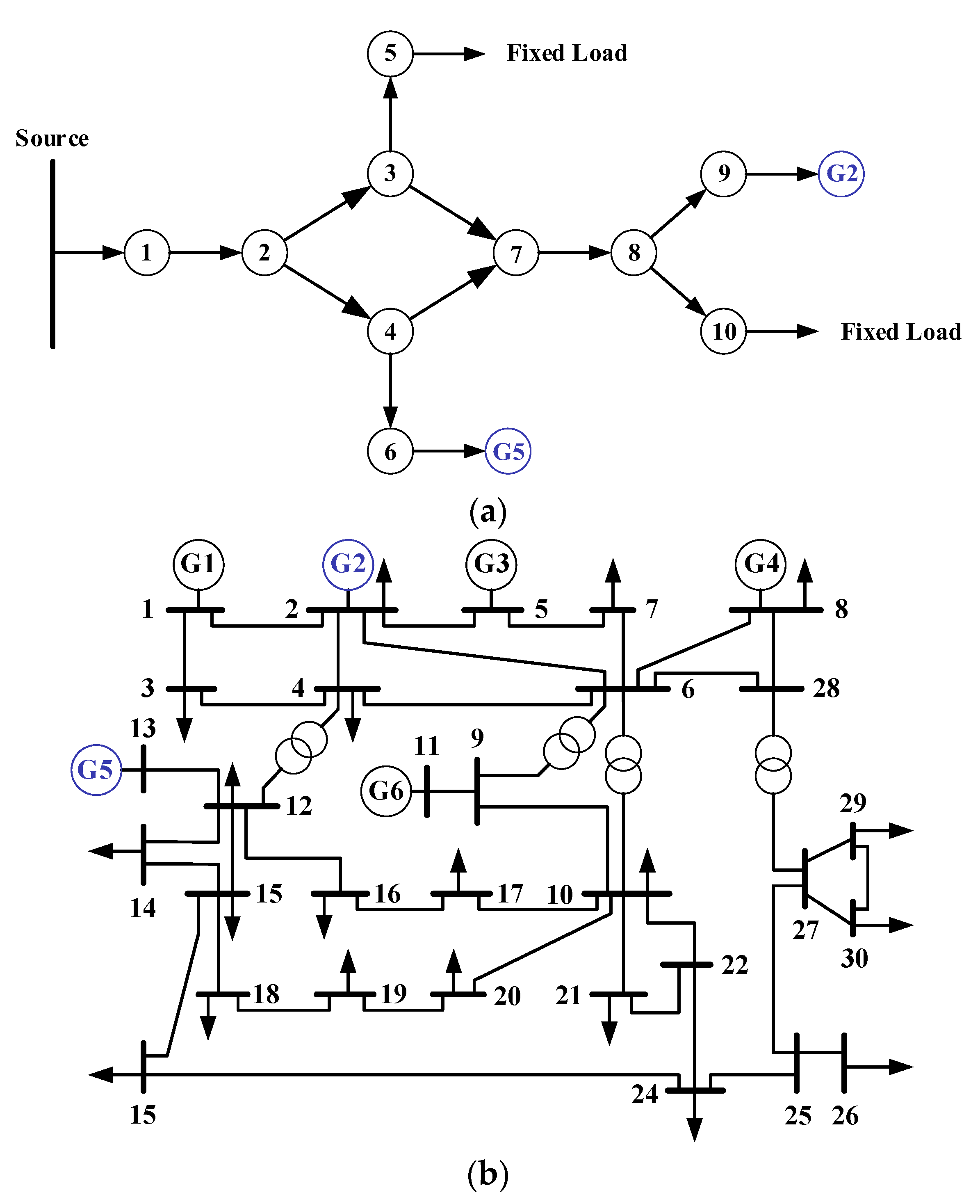
In the current experimental conditions, our method is validated on an integrated electricity-gas system shown in Figure 2, which is comprised of a 10-node natural gas network and the IEEE 30-bus system. In Figure 2, there are six generators in the electricity system, where G2, G5 are gas-fired generators. In the natural gas network, nodes five and ten are load nodes. Node six is connected to G5, and node nine is connected to G2.

Table 1. Natural gas operating parameters.

Term	Value	Term	Value	Term	Value
Z	0.9	R	500 J/(kg·K−1)	T	278 K

provides standard parameters of gas in the pipeline network,

Table 2. Node parameters of 10-node natural gas network.

Node	Gas Injection (kg/s)	Pressure (MPa)
5	−16.3	3.01
6	−11.8	3.04
9	−13.2	2.86
10	−18.7	2.93

gives the gas network parameters,

Table 3. 10-node natural gas network parameters.

Number	From	To	L (km)	f	d (m)	Mass Flow (kg/s)
1	1	2	10	0.01	0.5	60
2	2	3	20	0.012	0.4	34.6
3	2	4	15	0.011	0.45	25.4
4	3	5	10	0.01	0.5	16.3
5	3	7	15	0.011	0.45	18.3
6	4	6	10	0.01	0.5	11.8
7	4	7	20	0.012	0.4	13.6
8	7	8	5	0.01	0.4	31.9
9	8	9	5	0.01	0.4	13.2
10	8	10	5	0.01	0.4	18.7

shows the node parameters. The IEEE 30-bus system parameters are given by Matpower 4.0 [26]. We also simulate the integrated electricity-gas system to calculate the established state estimation model in MATLAB/Simulink (2021 version). MATLAB is an effective tool for simulating hybrid energy systems [27], which can, in combination with Matpower [28,29], be used to test and calculate the power flow of the power system. The widespread use of MATLAB in various energy system situations sufficiently demonstrates its effectiveness.

5.1. Case 1: The Correlation Coefficient ${\rho }_{\mathsf{\Delta }{\pi }_j^t,\mathsf{\Delta }{\dot{G}}_j^t}$ between Measurements $\mathsf{\Delta }{\pi }_j^t$ and $\mathsf{\Delta }{\dot{G}}_j^t$ and the Correlation Coefficient ${\rho }_{P_i,Q_i}$ between Measurements $P_i$ and $Q_i$ Are Set to 0.15

In this section, considering the existence of measurement correlations, our approach is used to estimate integrated electricity-gas system state. As shown in Figure 2, the natural gas network is connected to the electricity system through gas-fired generators G5 and G2 respectively, and nodes six and nine are supplied with gas by nodes four and eight respectively. Therefore, changes in gas flow at node six and node nine will result in changes in pressure of nodes four and eight. When gas demand of gas-fired generator G2 changes constantly, we track inlet pressure dynamic response of node 8. We set measurement correlation coefficients ${\rho }_{\mathsf{\Delta }{\pi }_j^t,\mathsf{\Delta }{\dot{G}}_j^t}$ and ${\rho }_{P_i,Q_i}$ in Equations (29) and (39) to 0.15, and set termination threshold $\epsilon$ in Equation (68) as $\epsilon ={10}^{-4}$. The gas flow of G2 at node 9 and pressure at node 8 are estimated with our method, and the results are compared with those of the Krawczyk operator (KO) interval method based on unscented transformation (UT). Krawczyk Operator (KO) is an iterative method that takes the interval vector obtained by the interval Gaussian elimination method as the initial value, and obtains the solution set of the interval linear equation by iterating the interval vector. The Krawczyk operator (KO) interval method based on unscented transformation (UT) mainly obtains the correlation between measurements through the symmetric sampling strategy of unscented transformation (UT), and describes and calculates the interval range where the correlation exists by using the Krawczyk operator (KO) interval method.

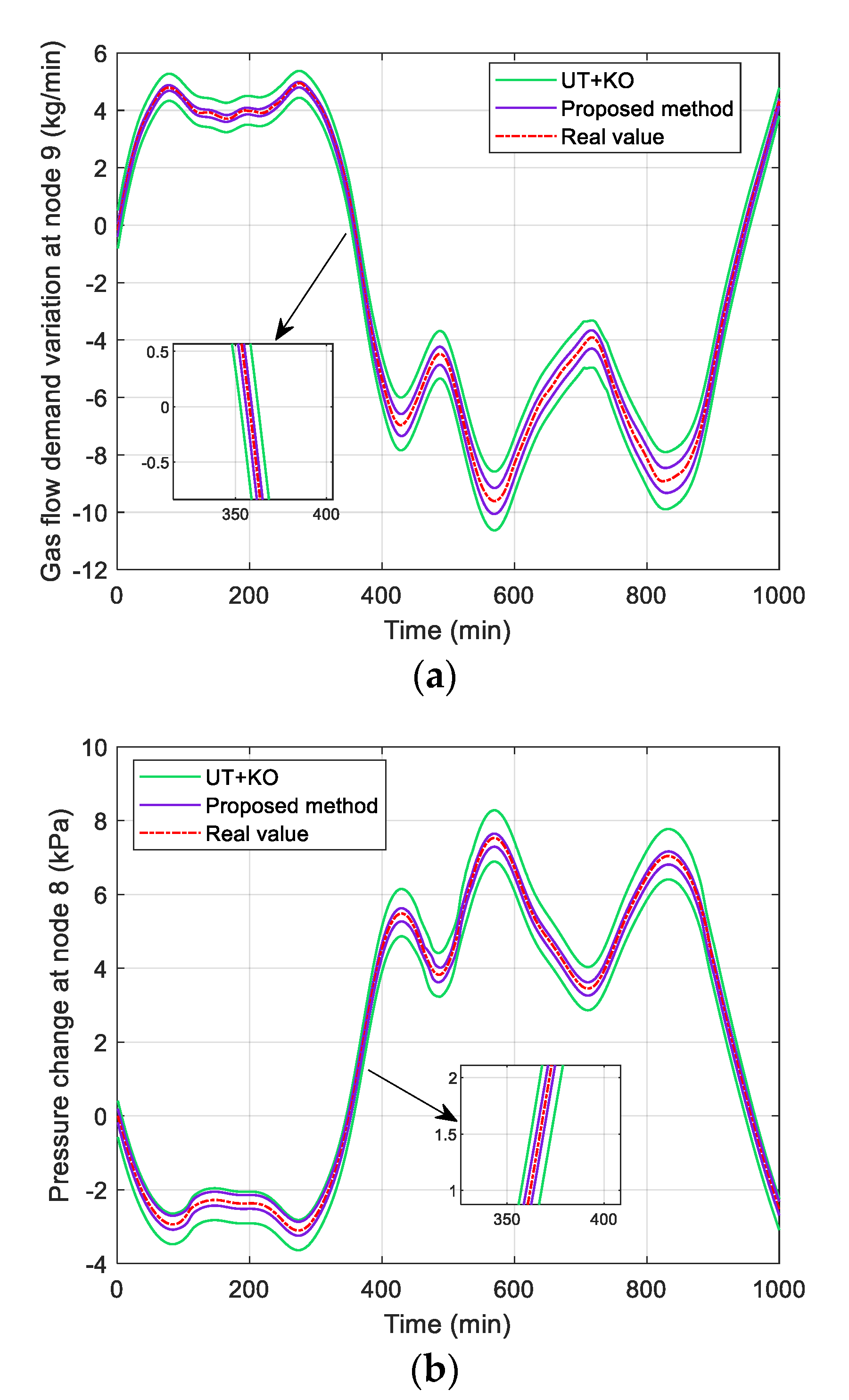
Figure 3 provides state estimation uncertainty ranges caused by measurement correlations obtained through the proposed method and UT+KO method. This paper mainly studies the slow change of natural gas flow. It can be intuitively seen that, compared with the UT+KO method, the interval boundary of the state variable of gas flow variation and pressure change given by the proposed method is more compact; while the interval upper boundary and lower boundary provided by the UT+KO method is far from real values, the interval range is larger. This is because UT requires independent calculation of measurements, and the KO interval method requires measurements to participate in multiple iterative operation. Multiple iterative operation of measurement interval at the same time will lead to the superposition and transmission of measurement correlations, which inevitably expands the interval range. These will easily exceed the operating limit of the system, thus losing the reference value.

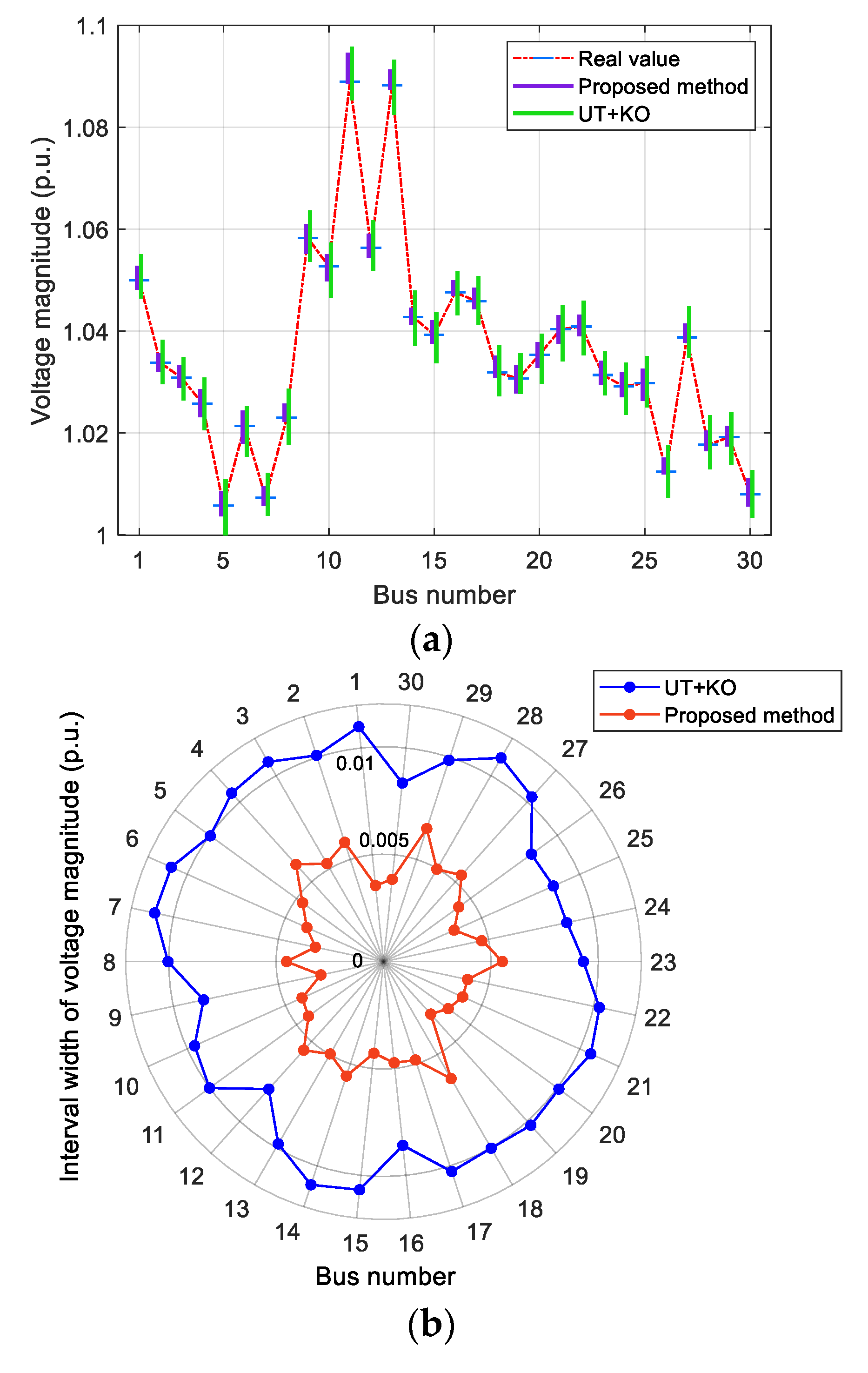
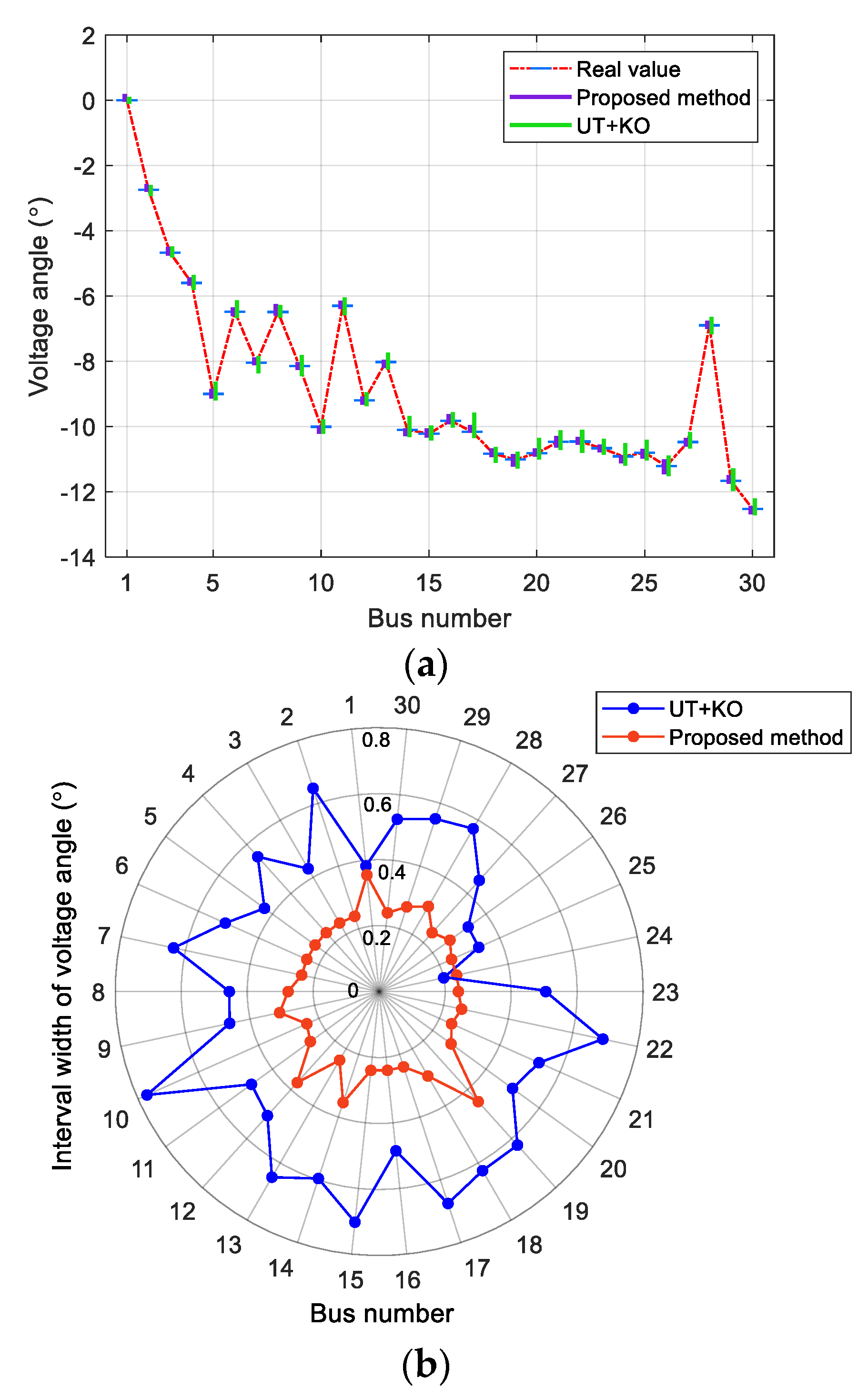
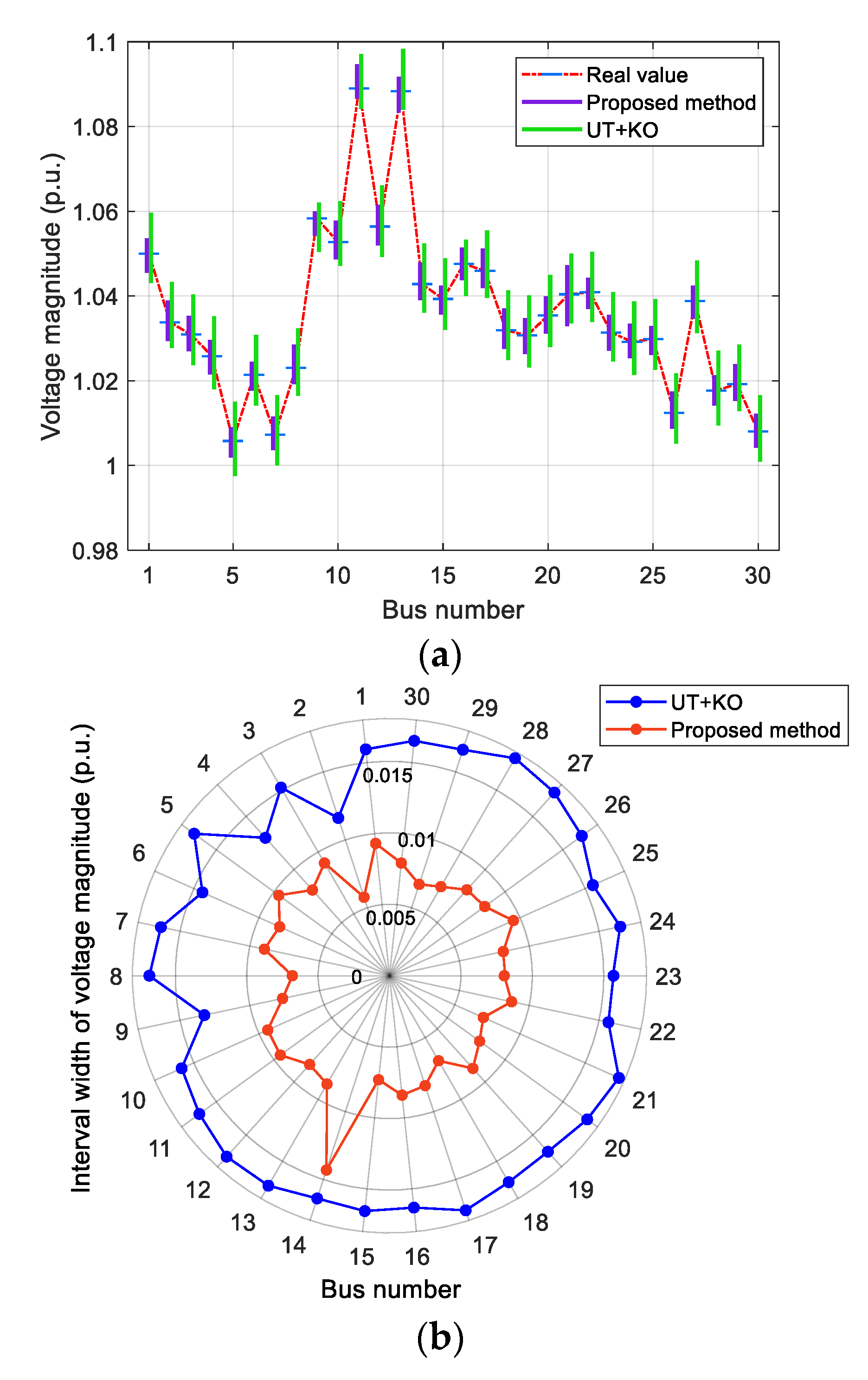
Then, the voltage magnitude and voltage angle of electricity system is estimated. Figure 4 and Figure 5 give voltage amplitude interval, voltage angle interval, and corresponding interval widths when the measurement correlation coefficient ${\rho }_{P_i,Q_i}=0.15$. In Figure 4a and Figure 5a, we use purple vertical lines to represent the voltage amplitude range obtained through the proposed method, green vertical lines to represent the results provided by the UT+KO method, and blue horizontal lines to represent the real value. In Figure 4b and Figure 5b, we highlight the voltage amplitude interval width and voltage angle interval width given by our method and UT+KO method in red and blue, respectively. Obviously, the upper boundary and lower boundary of interval obtained by our method are closer to real values, while interval range provided by the UT+KO method is larger, and the estimation results are somewhat conservative. This is mainly due to the superposition and transfer of measurement correlations of each measurement interval in the process of iterative calculation of multiple measurement intervals by the UT+KO method, which enlarges the interval and makes estimation results more conservative.

5.2. Case 2: The Correlation Coefficient ${\rho }_{\mathsf{\Delta }{\pi }_j^t,\mathsf{\Delta }{\dot{G}}_j^t}$ between Measurements $\mathsf{\Delta }{\pi }_j^t$ and $\mathsf{\Delta }{\dot{G}}_j^t$ and the Correlation Coefficient ${\rho }_{P_i,Q_i}$ between Measurements $P_i$ and $Q_i$ Are Set to 0.3

To further verify the effectiveness of our method at different measurement correlation levels, the measurement correlation coefficients ${\rho }_{\mathsf{\Delta }{\pi }_j^t,\mathsf{\Delta }{\dot{G}}_j^t}$ and ${\rho }_{P_i,Q_i}$ are set to 0.3, and the changes in gas flow demand and pressure at nodes are estimated, as shown in Figure 6.

In Figure 6, the estimated range of gas flow demand variation and pressure change at ${\rho }_{\mathsf{\Delta }{\pi }_j^t,\mathsf{\Delta }{\dot{G}}_j^t}=0.3$ is greater than that at ${\rho }_{\mathsf{\Delta }{\pi }_j^t,\mathsf{\Delta }{\dot{G}}_j^t}=0.15$ in Figure 3. The measurement correlation level therefore affects the estimation accuracy. When the measurement correlation is large, the upper bound and lower bound of estimation interval will deviate from the ideal state interval. Although state estimation interval range will increase as the measurement correlations increase, our method is superior to the UT+KO method.

Furthermore, we estimate the electricity system state when the measurement correlation coefficient ${\rho }_{P_i,Q_i}=0.3$; the results are shown in Figure 7 and Figure 8.

In Figure 7 and Figure 8, when measurement correlation coefficient ${\rho }_{P_i,Q_i}$ changes from 0.15 to 0.3, the estimated ranges of voltage magnitude and voltage angle expand. Both our method and the UT+KO method are affected to a certain extent, but the overall variation of our method is relatively small. This is because our method does not need to perform the iterative calculation of measurement interval at the same time, which avoids the accumulation and transmission of measurement correlations.

Furthermore, we evaluate the accuracy of results by using the following two indicators:

$$M_1=\frac{1}{n}{\displaystyle {\sum }_{i=1}^n\left({\overline{x}}_i-{\underset{\_}{x}}_i\right)}$$

(69)

$$M_2=\max \left({\overline{x}}_i-{\underset{\_}{x}}_i\right)$$

(70)

where ${\overline{x}}_i$ represents the upper boundary, and ${\underset{\_}{x}}_i$ represents the lower boundary of the interval variable, respectively. $M_1$ is the interval width average value, $M_2$ is the interval width maximum value. When $M_1$ and $M_2$ are smaller, accuracy is higher.

Table 4. Estimation accuracy (of the IEGS) of different measurement correlation coefficients.

Accuracy Indices		$\mathbf{The} \mathbf{Measurement} \mathbf{Correlation} \mathbf{Coefficients} {\mathit{\rho }}_{\mathit{\Delta }{\mathit{\pi }}_{\mathit{j}}^{\mathit{t}},\mathit{\Delta }{\dot{\mathit{G}}}_{\mathit{j}}^{\mathit{t}}}=0.15, {\mathit{\rho }}_{{\mathit{P}}_{\mathit{i}},{\mathit{Q}}_{\mathit{i}}}=0.15$		$\mathbf{The} \mathbf{Measurement} \mathbf{Correlation} \mathbf{Coefficients} {\mathit{\rho }}_{\mathit{\Delta }{\mathit{\pi }}_{\mathit{j}}^{\mathit{t}},\mathit{\Delta }{\dot{\mathit{G}}}_{\mathit{j}}^{\mathit{t}}}=0.3, {\mathit{\rho }}_{{\mathit{P}}_{\mathit{i}},{\mathit{Q}}_{\mathit{i}}}=0.3$
		${\mathit{M}}_1$	${\mathit{M}}_2$	${\mathit{M}}_1$	${\mathit{M}}_2$
Proposed method	Gas flow demand variation at node 9: $\mathsf{\Delta }{\dot{G}}_i^t$	0.3964	0.4541	0.5391	0.9308
UT+KO		0.8070	0.9681	1.2772	2.0476
Proposed method	Pressure change at node 8: $\mathsf{\Delta }{\pi }_i^t$	0.2749	0.3516	0.3704	0.6096
UT+KO		0.7523	0.7846	0.8961	1.3971
Proposed method	Voltage magnitude of IEEE 30-bus system: $V$	0.0046	0.0065	0.0084	0.0143
UT+KO		0.0099	0.0110	0.0161	0.0176
Proposed method	Voltage angle of IEEE 30-bus: ${\theta }_{ij}$	0.371	0.4486	0.4055	0.5495
UT+KO		0.527	0.7703	0.8143	1.0329

provides statistics for the estimation results of integrated electricity-gas system given by two methods, and provides the corresponding estimation accuracy indicators when the measurement correlation coefficient is 0.15 and 0.3, respectively. The results indicate that although estimation results accuracy decreases as the measurement correlation increases, the $M_1$ and $M_2$ indicators corresponding to the proposed method are smaller. This is mainly due to the accumulation of the measurement correlation of UT+KO method during the multiple iterative calculation of various measurement intervals, which enlarges interval range and reduces estimation results accuracy. In addition,

Table 5. IEGS computation time with different measurement correlation coefficients.

Method	Average Execution Time (s)
	$\mathbf{The} \mathbf{Measurement} \mathbf{Correlation} \mathbf{Coefficients} {\mathit{\rho }}_{\mathit{\Delta }{\mathit{\pi }}_{\mathit{j}}^{\mathit{t}},\mathit{\Delta }{\dot{\mathit{G}}}_{\mathit{j}}^{\mathit{t}}}=0.15, {\mathit{\rho }}_{{\mathit{P}}_{\mathit{i}},{\mathit{Q}}_{\mathit{i}}}=0.15$	$\mathbf{The} \mathbf{Measurement} \mathbf{Correlation} \mathbf{Coefficients} {\mathit{\rho }}_{\mathit{\Delta }{\mathit{\pi }}_{\mathit{j}}^{\mathit{t}},\mathit{\Delta }{\dot{\mathit{G}}}_{\mathit{j}}^{\mathit{t}}}=0.3, {\mathit{\rho }}_{{\mathit{P}}_{\mathit{i}},{\mathit{Q}}_{\mathit{i}}}=0.3$
Proposed method	2.68	3.41
UT+KO	43.59	54.37

provides the calculation time of our method and UT+KO method. It can be seen that when the measurement correlation coefficients are smaller, the average execution time is shorter. The UT+KO method uses multiple measurement intervals iterative calculation, so the calculation time is longer.

6. Conclusions

An interval state estimation method that considers the measurement correlations of electricity-gas systems is presented in this paper. The linear measurement model of electricity-gas systems is derived via Taylor series expansion, and the measurement variance-covariance matrix with measurement correlations is estimated. Then, the system parameter matrix and the measurement variance-covariance matrix with measurement correlations are combined into an interval, and the interval state matrix and linear equations of state estimation interval considering measurement correlations are constructed; as a result, the state estimation method for the electricity-gas system with measurement correlations is proposed. Finally, a method for determining state estimation interval range is presented. Comparing the state estimation interval with the safe operating limit range of the system will help system administrators to make effective judgments and effectively adjust electricity-gas systems. The numerical tests on an integrated electricity-gas system illustrate that our method outperforms the UT+KO method in terms of calculation accuracy and efficiency.

This paper quantifies and describes the measurement correlations of electricity-gas systems, but does not deeply consider the effects of measurement correlations on electricity-gas systems. In future work, we will further analyze the impacts of measurement correlations on electricity-gas systems, and will develop an adaptive interval state estimation method that dynamically adjusts the estimation process on the basis of real-time measurement data. This will improve the robustness and adaptability of interval state estimation, helping it to adapt to different working conditions and system changes.

References

1. Jiang, Y.; Ren, Z.; Yang, X. A steady-state energy flow analysis method for integrated natural gas and power systems based on topology decoupling. Appl. Energy 2022, 306, 118007. [Google Scholar] [CrossRef]
2. Aminifar, F.; Shahidehpour, M.; Fotuhi-Firuzabad, M. Power system dynamic state estimation with synchronized phasor measurements. IEEE Trans. Instrum. Meas. 2013, 63, 352–363. [Google Scholar] [CrossRef]
3. Muscas, C.; Pau, M.; Pegoraro, P.A. Effects of measurements and pseudomeasurements correlation in distribution system state estimation. IEEE Trans. Instrum. Meas. 2014, 63, 2813–2823. [Google Scholar] [CrossRef]
4. Santhosh, K.C.; Rajawat, K.; Chakrabarti, S. Robust distribution system state estimation with hybrid measurements. IET Gener. Transm. Distrib. 2020, 14, 3250–3259. [Google Scholar] [CrossRef]
5. Caro, E.; Conejo, A.J.; Minguez, R. Multiple bad data identification considering measurement dependencies. IEEE Trans. Power Syst. 2011, 26, 1953–1961. [Google Scholar] [CrossRef]
6. Zhao, J.; Wang, S.; Mili, L. A robust state estimation framework considering measurement correlations and imperfect synchronization. IEEE Trans. Power Syst. 2018, 33, 4604–4613. [Google Scholar] [CrossRef]
7. Singh, A.K.; Pal, B.C. Decentralized dynamic state estimation in power systems using unscented transformation. IEEE Trans. Power Syst. 2013, 29, 794–804. [Google Scholar] [CrossRef]
8. Caro, E.; Valverde, G. Impact of transformer correlations in state estimation using the unscented transformation. IEEE Trans. Power Syst. 2013, 29, 368–376. [Google Scholar] [CrossRef]
9. Zhao, J. Power system dynamic state estimation considering measurement correlations. IEEE Trans. Energy Conver. 2017, 32, 1630–1632. [Google Scholar] [CrossRef]
10. Zanni, L.; Le Boudec, J.Y.; Cherkaoui, R. A prediction-error covariance estimator for adaptive Kalman filtering in step-varying processes: Application to power-system state estimation. IEEE Trans. Contr. Syst. Technol. 2016, 25, 1683–1697. [Google Scholar] [CrossRef]
11. Lu, Z.; Gong, D.; Sun, Y. A New State Updating Approach in Power System Dynamic State Estimation Considering Correlated Measurements. In Proceedings of the 2017 Eighth International Conference on Intelligent Control and Information Processing (ICICIP), Hangzhou, China, 3–5 November 2017. [Google Scholar]
12. Lu, Z.; Wei, Z.; Sun, Y. Power system dynamic state estimation considering correlation of measurement error from PMU and SCADA. Concurr. Comp.-Pract. Exp. 2019, 31, e4726. [Google Scholar] [CrossRef]
13. Yang, Y.; Hu, W.; Min, Y. Projected unscented Kalman filter for dynamic state estimation and bad data detection in power system. In Proceedings of the 2017 Iet International Conference on Developments in Power System Protection, Copenhagen, Denmark, 31 March–3 April 2014. [Google Scholar]
14. Chakhchoukh, Y.; Vittal, V.; Heydt, G.T. PMU based state estimation by integrating correlation. IEEE Trans. Power Syst. 2013, 29, 617–626. [Google Scholar] [CrossRef]
15. Zhao, J.; Zhang, G.; Dong, Z.Y. Robust forecasting aided power system state estimation considering state correlations. IEEE Trans. Smart Grid. 2016, 9, 2658–2666. [Google Scholar] [CrossRef]
16. Chakhchoukh, Y.; Vittal, V.; Heydt, G.T. LTS-based robust hybrid SE integrating correlation. IEEE Trans. Power Syst. 2016, 32, 3127–3135. [Google Scholar] [CrossRef]
17. Lu, Z.; Yang, S.H.; Yang, S. Mixed measurement-based power system state estimation with measurement correlation. In 2016 Advances in Power and Energy Engineering: Proceedings of the 8th Asia-Pacific Power and Energy Engineering Conference; CRC Press: Boca Raton, FL, USA, 2016. [Google Scholar]
18. Caro, E.; Conejo, A.J.; Minguez, R. Power system state estimation considering measurement dependencies. IEEE Trans. Power Syst. 2009, 24, 1875–1885. [Google Scholar] [CrossRef]
19. Abedi, B.; Ghadimi, A.A.; Abolmasoumi, A.H. An improved TPM-based distribution network state estimation considering loads/DERs correlations. Electr. Eng. 2021, 103, 1541–1553. [Google Scholar] [CrossRef]
20. Valverde, G.; Saric, A.T.; Terzija, V. Stochastic monitoring of distribution networks including correlated input variables. IEEE Trans. Power Syst. 2012, 28, 246–255. [Google Scholar] [CrossRef]
21. Thorley, A.; Tiley, C.H.; Terzija, V. Unsteady and transient flow of compressible fluids in pipelines—A review of theoretical and some experimental studies. Int. J. Heat Fluid Flow. 1987, 8, 3–15. [Google Scholar] [CrossRef]
22. Osiadacz, A. Simulation of transient gas flows in networks. Int. J. Numer. Methods Fluids 1984, 4, 13–24. [Google Scholar] [CrossRef]
23. Abur, A.; Exposito, A.G.; Sun, Y. Power System State Estimation: Theory and Implementation; CRC Press: Boca Raton, FL, USA, 2004; pp. 79–93. [Google Scholar]
24. Sheikhi, A.; Bahrami, S.; Ranjbar, A.M. An autonomous demand response program for electricity and natural gas networks in smart energy hubs. Energy 2015, 89, 490–499. [Google Scholar] [CrossRef]
25. Liu, Y.; Wang, Y.; Zhang, N. A data-driven approach to linearize power flow equations considering measurement noise. IEEE Trans. Smart Grid. 2019, 11, 2576–2587. [Google Scholar] [CrossRef]
26. Zimmerman, R.D.; Murillo-Sánchez, C.E.; Thomas, R.J. MATPOWER: Steady-state operations, planning, and analysis tools for power systems research and education. IEEE Trans. Power Syst. 2010, 26, 12–19. [Google Scholar] [CrossRef]
27. Xu, X.; Jia, H.; Chiang, H.D. Dynamic modeling and interaction of hybrid natural gas and electricity supply system in microgrid. IEEE Trans. Power Syst. 2014, 30, 1212–1221. [Google Scholar] [CrossRef]
28. Xu, J.; Wu, Z.; Dou, X. An interval arithmetic-based state estimation for unbalanced active distribution networks. In Proceedings of the 2017 IEEE Power & Energy Society General Meeting, Chicago, IL, USA, 16–20 July 2017. [Google Scholar]
29. D’Antona, G. Power system static-state estimation with uncertain network parameters as input data. IEEE Trans. Instrum. Meas. 2016, 65, 2485–2494. [Google Scholar] [CrossRef]
Figure 1. Schematic diagram of natural gas flow inside the pipeline.
Energies 17 00755 g001
Figure 2. The integrated electricity-gas system comprising 10-node natural gas network and IEEE 30-bus system. (a) Topology of 10-node natural gas network; (b) Topology of IEEE 30-bus system.
Energies 17 00755 g002
Figure 3. State estimation interval bound of the natural gas system, considering the measurement correlation coefficient ρ Δ π j t , Δ G ˙ j t = 0.15 . (a) Gas flow demand variation; (b) Pressure change.
Energies 17 00755 g003
Figure 4. State estimation interval bound of IEEE 30-bus system with measurement correlation coefficient ρ P i , Q i = 0.15 . (a) Voltage magnitude; (b) Interval width of voltage magnitude.
Energies 17 00755 g004
Figure 5. State estimation interval bound of IEEE 30-bus system with measurement correlation coefficient ρ P i , Q i = 0.15 . (a) Voltage angle; (b) Interval width of voltage angle.
Energies 17 00755 g005
Figure 6. State estimation interval bound of natural gas system with measurement correlation coefficient ρ Δ π j t , Δ G ˙ j t = 0.3 . (a) Gas flow demand variation; (b) Pressure change.
Energies 17 00755 g006
Figure 7. State estimation interval bound of IEEE 30-bus system with measurement correlation coefficient ρ P i , Q i = 0.3 . (a) Voltage magnitude; (b) Interval width of voltage magnitude.
Energies 17 00755 g007
Figure 8. State estimation interval bound of IEEE 30-bus system with measurement correlation coefficient ρ P i , Q i = 0.3 . (a) Voltage angle; (b) Interval width of voltage angle.
Energies 17 00755 g008