Abstract
Supermarket refrigeration systems are integral to food security and the global economy. Their massive scale, characterized by numerous evaporators, remote condensers, miles of intricate piping, and high working pressure, frequently leads to problematic leaks. Such leaks can have severe consequences, impacting not only the profits of the supermarkets, but also the environment. With the advent of Industry 4.0 and machine learning techniques, data-driven automatic fault detection and diagnosis methods are becoming increasingly popular in managing supermarket refrigeration systems. This paper presents a novel leak-detection framework, explicitly designed for supermarket refrigeration systems. This framework is capable of identifying both slow and catastrophic leaks, each exhibiting unique behaviours. A noteworthy feature of the proposed solution is its independence from the refrigerant level in the receiver, which is a common dependency in many existing solutions for leak detection. Instead, it focuses on parameters that are universally present in supermarket refrigeration systems. The approach utilizes the categorical gradient boosting regression model and a thresholding algorithm, focusing on features that are sensitive to leaks as target features. These include the coefficient of performance, subcooling temperature, superheat temperature, mass flow rate, compression ratio, and energy consumption. In the case of slow leaks, only the coefficient of performance shows a response. However, for catastrophic leaks, all parameters except energy consumption demonstrate responses. This method detects slow leaks with an average F1 score of 0.92 within five days of occurrence. The catastrophic leak detection yields F1 scores of 0.7200 for the coefficient of performance, 1.0000 for the subcooling temperature, 0.4118 for the superheat temperature, 0.6957 for the mass flow rate, and 0.8824 for the compression ratio, respectively.
1. Introduction
In Canada, there are over 5000 large supermarkets, and each consumes about 5000 megawatt hours (MWh) of electricity annually. Cumulatively, their energy consumption approximates 25 terawatt hours (TWh) per year, which equates to the annual output of three large power plants [1,2]. This massive energy usage underscores the position of supermarkets as among the most energy-demanding types of commercial buildings [3].
Even though they meet the standard heating, ventilation, and air conditioning (HVAC) requirements, refrigeration systems in supermarkets are responsible for approximately half of their total energy consumption [3]. This level of usage translates to an annual energy cost of around $150,000 for refrigeration in a large supermarket. In terms of scale, these energy costs equate to nearly 1% of total supermarket sales. This is a significant expenditure, particularly considering the supermarket’s average net profit margin is also around 1%. Therefore, under standard operating conditions, a decrease in energy costs by 10% could potentially lead to an approximate 10% rise in profits [1]. Therefore, optimizing the refrigeration system has a significant positive impact on both the environment and the profitability of these businesses.
In 2018, Behfar et al. [4] comprehensively analysed common operating faults and equipment characteristics in supermarket refrigeration systems. Utilizing expert surveys, facility management system messages, service calls, and service records, their study revealed that refrigerant charge problems (leaks and overcharging) are the most common cause of equipment failure in supermarkets. Typically, a supermarket refrigeration system houses refrigerants between 3000 to 5000 lb in a closed circuit [4,5]. Annually, leak rates can average around 11%, spiking up to 30% in certain situations [6]. Leaks in refrigeration systems can originate from four distinct sources. The first type is a gradual leakage through components over time, which often remains undetected until the leak becomes substantial. The second type is catastrophic or physical damage, resulting in significant refrigerant losses within a short period. A third source of leaks can be the activation of pressure relief devices. Lastly, small but consistent losses may occur during routine maintenance, repair, and refrigerant recovery, contributing to the overall leakage [6]. These leaks in supermarkets lead to significant direct and hidden costs, including lost sales from perishable items, increased refrigerant expenses, compliance fines, higher energy consumption, food spoilage, and impacts on employee satisfaction and customer loyalty. Therefore, the economic impact of such outages can be much higher than the direct maintenance costs [7]. Apart from these economic losses, refrigerant leaks have a direct impact on the environment as well. While nearly all newly constructed supermarket stores have moved away from using Hydrofluorocarbons (HFCs), these still remain the predominant refrigerants in existing supermarkets [6]. HFCs pose a substantial environmental challenge, given their atmospheric lifespan, which can extend up to 14 years. Regulatory authorities worldwide have implemented stricter regulations regarding leak repair and store inspections in order to address this urgent issue. These new regulations encourage advanced monitoring techniques [8,9,10]. Moreover, considering the regulations for environmental protection and food safety, along with the costs associated with refrigerant loss, the early detection of leaks in supermarket refrigeration systems is critically important. As a result, research into refrigerant leakage has gained substantial attention.
With the advent of Industry 4.0 [11], fault detection and diagnosis (FDD) tasks, which were typically performed by humans, are being transformed into automatic fault detection and diagnosis (AFDD) through the use of data-driven methods. Although many AFDD methods have been developed for air conditioning and chillers [12,13,14], comparatively little attention has been paid to commercial supermarket refrigeration systems. While basic refrigeration cycles are similar, supermarket refrigeration systems and chillers differ in many aspects. AFDD methods for industrial systems typically function by monitoring specific performance indices or features that are sensitive to a particular fault. When a performance index significantly deviates from its expected value or exceeds a predetermined threshold, the AFDD method can detect the presence of a fault [15,16,17,18,19,20,21,22,23]. In other cases, it is addressed as a classification problem [24]. However, due to the limited availability of faulty data in real-world scenarios, a significant class imbalance exists when one tries to use the classification approach with actual data.
Utilizing power consumption as a sensitive feature is a prevalent approach in the AFDD solutions for detecting leaks in supermarket refrigeration systems. Fisera and Stluka [22] proposed an anomaly detection model using a regression-based approach that explored power consumption data that was fused with some additional sensor data. After being trained on non-faulty data, the model, upon encountering faulty data, produced prediction errors due to the disruption in the relationship between the input variables. Mavromatidis et al. [21] leveraged an Artificial Neural Network (ANN) to predict energy consumption, and used thresholds to detect faults. Srinivasan et al. [16] presented an approach to detect anomalous behaviours, including refrigerant leaks, by monitoring their energy signals alone. They employed a seasonal autoregressive integrated moving average (SARIMA) model and a regression model. They further incorporated additional sensors to reduce false positives, and they used the refrigerant level at the receiver for leak detection.
Aside from power consumption, a few studies have focused on using parameters that exhibit thermodynamic behaviour changes in a system, including variations in temperature, pressure, mass flow rate, and heat transfer rates. Yang et al. [25] employed Kalman Filter and Extended Kalman Filter techniques to generate residuals, which were then analysed to detect and isolate four types of sensor faults: drift, offset, freeze, and hard-over, specifically for two temperature sensors. The detection was conducted by comparing the residual to a predetermined threshold. A cumulative sum (CUSUM) method was used for residual evaluation to enhance the clarity of the residual deviation. In a subsequent study, Yang et al. [26] expanded on fault detection and isolation in supermarket refrigeration systems by introducing the Unknown Input Observer method, which is capable of detecting both sensor and parametric faults. While these studies did not explicitly focus on refrigerant leak detection, their approach to sensor fault detection and isolation could potentially be applied to leak detection in refrigerators. This depends on the specific characteristics of the leak and its impact on the sensors.
Assawamartbunlue and Brandemuehl [17] used the Refrigerant Leak Index (RLI) parameter for their study. They developed a probabilistic approach to detect refrigerant leakage in supermarket refrigeration systems. The authors created a belief network model that predicts the liquid volume fraction in the receiver, utilizing seven variables derived from measured data and the average temperatures of refrigeration cases. The RLI values, calculated from the difference between the predicted and observed liquid volume fractions, served as the target variable for leak detection. Moreover, they constructed an ANN model to make the technique faster and more practical for field implementation with small microcomputers. Their study provides a unique perspective on using probabilistic models and neural networks for leak detection in supermarket refrigeration systems. In a different study, Wichman and Braun [20] presented a decoupling-based diagnostic method for detecting faults, including refrigerant leaks in commercial coolers and freezers. This method uses decoupling features and parameters uniquely influenced by individual faults to manage multiple simultaneous faults. They used the difference between the superheat and subcooling temperature values as the undercharge faults’ decoupling feature. Their study explained the potential of this method for real-world applications, but also emphasized the need for further research to improve the decoupling of certain features, such as refrigerant charge problems, from other faults.
Behfar et al. [18] examined the potential of AFDD methods in supermarket systems. They evaluated two distinct AFDD methods: a rule-based method and a data-driven method. The rule-based method, originally developed for HVAC systems [27], exhibited sensitivity to certain faults, like a broken condenser fan and the first lighting fault scenario. However, it was less sensitive to undercharge fault scenarios. On the other hand, the data-driven method [21] effectively detected changes in energy consumption, but was less effective when input variables fluctuated significantly during normal operation. The authors suggested that future research could improve fault detection in supermarket refrigeration systems by combining data-driven methods with more detailed input data, such as pressure and temperature measurements and control modes. They also proposed weighing the diagnostic inputs to enhance the effectiveness of the AFDD methods. They provided valuable insights to improve AFDD methods for the detecting of leaks and other faults in supermarket refrigeration systems.
This paper introduces a novel leak detection framework that is explicitly tailored for supermarket refrigeration systems. The main contributions of this paper can be summarized as follows:
- A robust leak-detection framework designed for supermarket refrigeration systems: None of the existing solutions detect both slow and catastrophic leaks, which show two contrasting behaviours and should be treated differently.
- A framework that is independent from the refrigerant level sensor of the receiver tank: Most existing solutions rely on the refrigerant level sensor of the receiver tank, which is unavailable in most supermarkets. Instead, this proposed solution relies only on the thermodynamic properties and energy data available in any supermarket refrigeration system.
- Use of a false alarm mitigation mechanism: None of the existing solutions for leak detection in supermarket refrigeration systems have implemented a false alarm mitigation mechanism to improve accuracy, even during the transition of the system’s control modes.
The remainder of the paper is organized as follows. Section 2 gives brief background information on the proposed approach, and Section 3 describes the methodology followed for catastrophic and slow leak detection. Section 4 presents the results of the proposed algorithms using real-world data obtained from supermarkets in Canada. Finally, the conclusions are explained in Section 5.
2. Background
This paper presents a prediction-based anomaly detection model specifically designed to identify leaks in supermarket refrigeration systems. This section provides an overview of the relevant background information related to supermarket refrigeration systems and categorical gradient boosting regressors.
2.1. Supermarket Refrigeration Systems
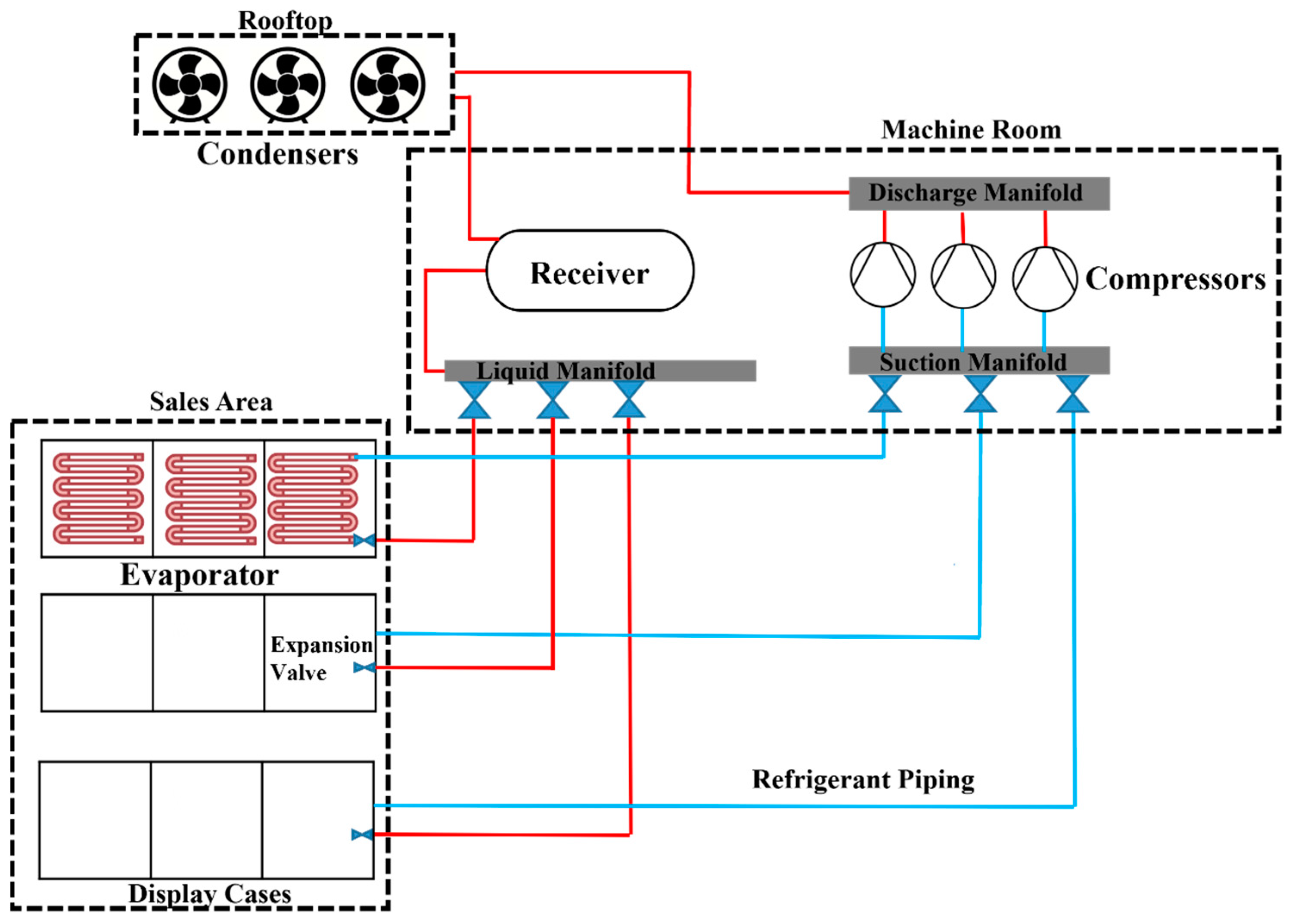
Supermarket refrigeration has become a vital aspect of modern society because it allows for preserving and storing perishable items, improving food safety, reducing food waste, and streamlining the supply chain. Figure 1 presents a schematic diagram of a typical supermarket refrigeration system comprising four primary components: the compressor, condenser, expansion valve, and evaporator [28,29,30]. The compressor and expansion valves are in the mechanical room, whereas the condenser is on the rooftop. Evaporators are found in display cases and walk-in coolers/freezers, where the internal temperatures vary according to the stored products. For instance, in medium-temperature display cases, beverage coolers and dairy cases are typically kept at around 2 °C, whereas low-temperature display cases need to retain frozen food at a temperature as low as −26 °C. The heat loads of multiple display cases are combined into one compressor/condenser system in order to maintain the desired temperature.

Figure 1.
Schematic diagram of a typical supermarket refrigeration system. Red represents the high-pressure side of the piping system, whereas blue indicates the low-pressure side.
The supermarket refrigeration cycle can be summarized as follows [29]:
- I.
- Activation signal from control system: The control system activates one or more compressors to begin the refrigeration cycle.
- II.
- Compressor intake: The compressors pull low-pressure evaporated refrigerant gas from a common suction line.
- III.
- Compression: The refrigerant gas is compressed, generating superheated, high-pressure gas.
- IV.
- Gas discharge: The condenser(s) receives the superheated gas from the compressors through a common discharge line.
- V.
- Condensation: The high-pressure gas rapidly loses heat while going through a phase change to become a high-pressure liquid refrigerant.
- VI.
- Refrigerant storage: The high-pressure liquid refrigerant is stored in a receiver.
- VII.
- Distribution: The liquid refrigerant enters the evaporators of multiple display cases.
- VIII.
- Expansion valve control: Each evaporator has a locally controlled expansion valve that controls the flow and pressure of the refrigerant.
- IX.
- Evaporation: As the liquid refrigerant turns into a gas, the evaporator coil cools, and the refrigeration cases cool.
- X.
- Individual System Pressure Regulation: Most supermarket systems have an individual suction pressure control valve for each system, so that each system can run at the pressure required to maintain its specific temperature setpoint.
- XI.
- Monitoring of pressure: The number of active compressors, or their operating speed, if variable, are controlled to maintain steady suction pressure (or, if enabled, float the pressure up to optimize energy).
Supermarket refrigeration systems exhibit complexity due to various factors influencing their design, operation, and maintenance. The key factors contributing to this complexity are the need to accommodate fluctuating load demands, the requirement for multiple temperature zones, the implementation of sophisticated control strategies and optimization techniques, and the challenges associated with regular maintenance and servicing.
2.2. Categorical Gradient Boosting Regressor
The categorical gradient boosting (CatBoost) algorithm [31] is an improved gradient decision tree version that can handle categorical features well. CatBoost has been used in various fields, including finance [32] and also to analyse time series data [33,34,35]. CatBoost uses decision trees as the base predictor and uses gradient boosting. The boosting approach sequentially combines many weak models that perform slightly better than a random chance method in order to create a robust predictive model using a greedy search. By fitting decision trees one after the other, each tree learns from the mistakes of its predecessors, thereby reducing errors. This process of adding new functions to existing ones continues until the selected loss function reaches a minimum, resulting in an optimized model. Unlike other gradient-boosting models, CatBoost employs oblivious trees in the decision tree-growing procedure. An oblivious tree is a type of decision tree where each level of the tree is based on a single feature, ensuring that every path through the tree uses the same features in the same order [36]. This uniformity allows for that calculation of the index of the leaf using bitwise operations. The use of oblivious trees not only simplifies the fitting process, making it more efficient on CPUs, but the consistent structure of the tree also acts as a form of regularization, helping to find an optimal solution and preventing the model from overfitting [31].
CatBoost distinguishes itself from other gradient-boosting algorithms through three unique features. Firstly, it employs ordered boosting, an innovative modification of traditional gradient boosting, to overcome the problem of target leakage. Secondly, the algorithm is designed to be applied to small datasets without leading to overfitting. Finally, CatBoost is particularly adept at handling categorical features, ensuring minimal information loss. This handling is typically accomplished during preprocessing, where original categorical variables are substituted with one or more numerical values.
3. Methodology
Modern supermarket refrigeration systems possess a plethora of probes to collect data, covering the entire refrigeration process from the compressor, condenser, and expansion valve to the display cases. The focus of this study is primarily on the typical sensor values that are common in most supermarket refrigeration systems. Most operational data in a typical supermarket refrigeration system is highly susceptible to external ambient temperature and humidity. Supermarket refrigeration systems function in various modes, leading to fluctuations in operational data as the system transitions between these conditions. For instance, there are regular defrosting cycles, changes in the state of the heat reclaim valve, and alternating split states in the condenser. Therefore, relying on raw sensor data values for anomaly detection can result in many false positives, as these operational mode changes can mimic or mask genuine anomalies [20]. Therefore, a prediction-based anomaly detection model incorporating these external factors has been developed to accurately identify true anomalies. The CatBoost regressor is chosen for time series prediction, due to its promising capabilities for short-term predictions, its robustness to outliers, its ability to capture non-linear relationships, and a reduced risk of overfitting. Moreover, the CatBoost regressor demonstrates better performance for this data than other similar models like XGboost and LightGBM. There are two major types of leaks that occur in supermarket refrigeration systems: catastrophic leaks and slow leaks. Separate algorithms have been developed to detect each type of leak under the umbrella of a single framework.
3.1. Data Preprocessing and Feature Engineering
The data for this study are collected from various supermarkets in Canada with HFC as the refrigerant. Due to the confidentiality reasons, the names of the supermarkets cannot be disclosed, and therefore code names such as Supermarket 1 and Supermarket 2 are used in this paper. Past leak events are identified through a comprehensive approach that combines analysing data, expert insights, service records, and customer complaints, effectively detecting slow and catastrophic leaks. The datasets are then carefully extracted from different supermarkets to include 3–6 months of data. These datasets are selected to have normal non-leak operational data before and after the leak event.
Typically, companies maintaining supermarket refrigeration systems manually analyse vast data streams from these systems to detect leaks. With domain expertise and references to the refrigeration literature [23,37,38], critical parameters for the proposed model are identified and listed in Table 1. However, the industrial dataset presented practical challenges. For instance, some stores have probes to gather specific parameters, while others do not. Additionally, some parameters have numerous missing values and noise, rendering them almost unusable. Using the available data and employing the thermodynamic library named CoolProp [39], a set of new features is created to gain insights into the thermodynamic behaviour of the system, as shown in Table 2.

Table 1.
Data collected from the supermarket refrigeration systems.
Table 2.
Newly calculated parameters using operational data.
The refrigerant level value at the receiver has not been used for any modelling, since it is not available in all supermarkets. Additionally, feature engineering techniques are employed to extract time series-specific features. These include lagged values, cyclic encoding of the hour of the day for daily seasonality, and cyclic encoding of the day of the week for weekly seasonality.
For each dataset, a partial correlation analysis is performed for each target parameter to select appropriate input features and mitigate the effect of multicollinearity. Autocorrelation function (ACF) and partial autocorrelation function (PACF) plots are analysed to determine the optimal number of lagged features required for the model. Figure 2a,b depict the ACF and PACF plots of an input feature, and Figure 2c,d show the ACF and PACF plots of a target feature, respectively. A significant autocorrelation is also observable at the 96th lagged value, corresponding to the same time on the previous day. Moreover, L2 regularization is used to prevent overfitting.
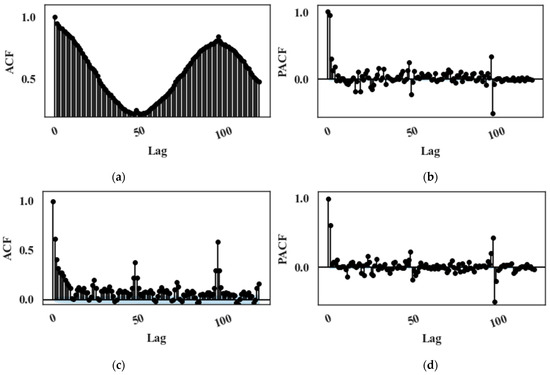
Figure 2.
(a) The ACF plot and (b) the PACF plot of down leg temperature (an input variable), (c) the ACF plot and (d) the PACF plot of mass flow rate (a target variable).
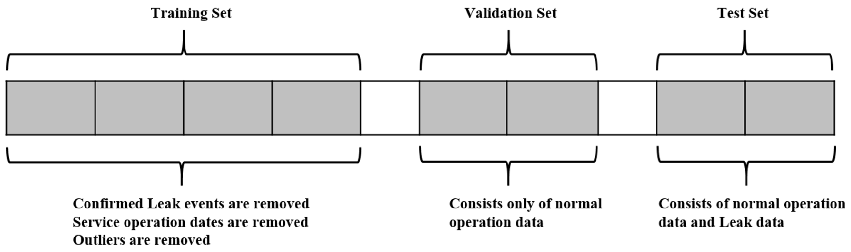
The leak events, service incidents, and other special events (e.g., power outages) are identified first for a given dataset. Then, the dataset is divided into training, validation, and test sets. Usually, a test set is selected to include a leak event. Therefore, only one month of data is used to detect catastrophic leaks, and, for slow leak detection, two months of data are selected in the test set. The training and validation sets are selected to include only normal (non-leak) operation data without outliers. Depending on the availability of data, two to three months of data are used for the training set, while fifteen to thirty days of data are used for the validation set. A gap is maintained between each set to stop the possibility of data leakage due to the use of the lagged values (Figure 3).

Figure 3.
Training, validation, and test set split strategy (not to the scale).
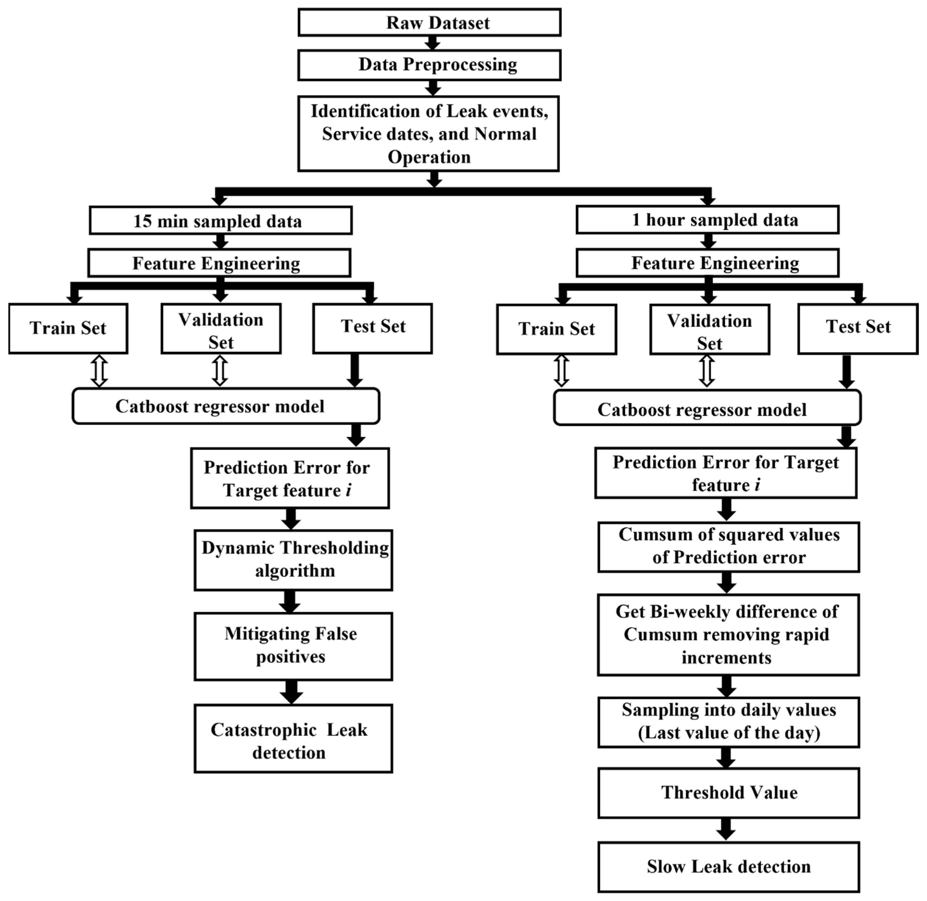
Earlier in-depth analyses were conducted by Tassou and Grace [23,37], and Cho et al. [40] investigated how various operational characteristics are affected by changes in the refrigerant levels, particularly in chillers and transcritical CO2 heat pumps, equipped with a flash tank. Their research indicated that the coefficient of performance (COP), superheat temperature, subcooling temperature, mass flow rate, compression ratio, and power consumption respond to the changes in the refrigerant level. Furthermore, Fisera and Stluka [22] emphasised the potential use of parameters like COP for system-level fault detection in supermarket refrigeration systems. Therefore, in this proposed solution, COP, superheat temperature, subcooling temperature, mass flow rate, compression ratio, and power consumption are selected as the target features when developing prediction models. Figure 4 shows the overall architecture of the proposed algorithm.

Figure 4.
Overall algorithm architecture for leak detection.
3.2. Catastrophic Leak Detection
Catastrophic leaks involve the rapid release of refrigerants from a refrigeration system, often due to equipment failure. Since the system loses a significant amount of refrigerant during a catastrophic leak event within a short period of time, there is a rapid fluctuation in system parameters. In modern supermarket systems, catastrophic leaks are rare, namely due to consistent and proactive maintenance. However, they are still possible due to their massive scale. This paper proposes a prediction-based anomaly detection algorithm to detect catastrophic leaks, using 15 min sampled data. A CatBoost regression model is used for prediction, and a novel non-parametric dynamic thresholding method is used for anomaly detection.
A CatBoost regression model is trained using non-leak data to accurately predict the target variable during normal operation. Lagged values of operational data (including temperature, pressure, energy, and calculated thermodynamic data), feature-engineered data to extract time-series information, system status changes, and both outdoor and indoor humidity and temperature values are compiled into a tabular format. This serves as input for the CatBoost regression model. Prediction error values are obtained in real-time and are fed into the anomaly detection algorithm. Due to the complexity of the system, these prediction error values always contain noise, and the anomaly detection algorithm must be capable of distinguishing anomalies from this noise. A non-parametric dynamic thresholding algorithm, proposed by Hundman, Kyle et al. [41], is used to detect these anomalies. This proposed algorithm comprises the following steps: (1) dynamic error thresholding and (2) false positive mitigation.
3.2.1. Dynamic Error Thresholding
At time step , a prediction error value is evaluated as , and the error series defined as , where symbolizes the length of past error values window applied to assess current errors.
Setting an appropriate threshold for the error value series is necessary to reliably identify anomalies. Initially, an exponentially weighted average technique is used to generate the smoothed error series; is used to get rid of the sharp spikes. Then, a set of potential threshold values is generated, as follows in Equation (1):
Each possible threshold is determined as shown in Equation (2):
here, represents the tolerance level of the threshold in terms of the number of standard deviations away from , generally ranging from 2 to 10. The optimal threshold is given by Equation (3):
where:
Once is identified, it allows for the most effective separation between normal and abnormal data. This approach also curtails any excessive bias towards the abnormal data, preventing overly eager behaviour. Finally, an anomaly score is assigned to all the values in in , which are above , to indicate the severity of the anomaly. The anomaly score () is calculated as in Equation (4):
3.2.2. Mitigating False Positives
Since the prediction error is noisy, there is a risk of having plenty of false positives. To deal with this issue, an extra vector is introduced, comprising the highest value from each anomalous subsequence, organized in a descending manner, that is,
The maximum smoothed error that is not classified as an anomaly is also added to the end of the vector, specifically . When incrementally traversing through the sequence, for each step within , is calculated using Equation (6), which denotes the percentage reduction between subsequent errors in :
Another threshold is designated as the expected minimum percentage decrease. If at any step , is surpassed by , then all the errors where and their corresponding anomaly sequences are affirmed as anomalies. Conversely, if and the same condition is applicable for all , the associated error sequences are re-categorized as normal. The accurate selection of the threshold ensures a clear differentiation between errors arising from regular noise within the stream and genuine anomalies that have occurred in the system.
3.3. Slow Leak Detection
Slow leaks are both the most common and the most challenging type of leak to detect. Such leaks do not significantly affect the operational characteristics or the efficiency of the system until a substantial amount of refrigerant has leaked out. Consequently, it requires a different approach to detect slow leaks. A proposed approach for slow leak detection involves a combination of empirical observations and predictive modelling. There is an observable shift in the partial correlation coefficient between the input variables (X) and the target variables (Y), as the system transitions from a non-leak state to a leaked state. The partial correlation coefficient is then calculated, taking into account any confounding variables, such as the indoor and outdoor temperature and humidity.
The CatBoost regression model is used to construct the predictive model , utilizing the 1 h sampled data, thus establishing the relationship during normal operations, where denotes the residual error. As the system enters a slow leak state, changes in the correlations between and result in the prediction error given in Equation (7):
The squared error is accumulated over time, forming the cumulative sum of squared errors () The bi-weekly rise () of the is computed from the hourly data, given in Equation (8), where represents the current hour and represents the hour exactly two weeks prior:
Gradient of and the rolling mean and the standard deviation of the gradient are calculated over a two-week window. Rapid increases in values are identified when . The amount of rapid increase and the bi-weekly sum of rapid increases are computed. The bi-weekly rise, which is due to gradual increases , is then calculated, as shown in Equation (9):
Finally, a new time series () is generated by resampling the data to daily intervals. This is completed by taking the final value of in each day. It focuses on the longer-term, more gradual changes in cumulative squared errors. The proposed detection strategy sets a threshold () for . Under normal operation, remains consistent without any trend, but with the onset of a slow leak, tends to increase. The slow leak detection criterion is thus: if , a slow leak is likely to be present. The selection of involves a trade-off between minimizing false positives and ensuring early detection of slow leaks.
3.4. Model Evaluation
3.4.1. Accuracy of Prediction Model during Non-Leak Operations
During the non-leak operation, the prediction model should be able to predict the modelled target parameter with a minimum prediction error. The mean absolute percentage error (MAPE) and the R2 Score are used to measure the performance of the prediction model (Equations (10) and (11)):
where:
- is the total number of data points;
- is the actual value for the observation;
- is the predicted value for the observation.
Furthermore, keeping the false alarm rate (FAR) to a minimum for the non-leak data is essential. This can be represented by the following equation, where FP stands for false positives, and TN represents true negatives:
3.4.2. Accuracy of the Anomaly Detection Model
To measure the performance and utility of the proposed anomaly detection model, TP, TN, FP, and FN are first calculated, providing fundamental insight into the model’s ability. Then, the precision, recall, and F1 Scores (Equations (13)–(15)) are calculated. Lastly, the time to detect the leak metric is crucial in assessing the model’s timeliness and efficiency in recognizing leaks, a factor of paramount importance in preventing substantial damage or loss.
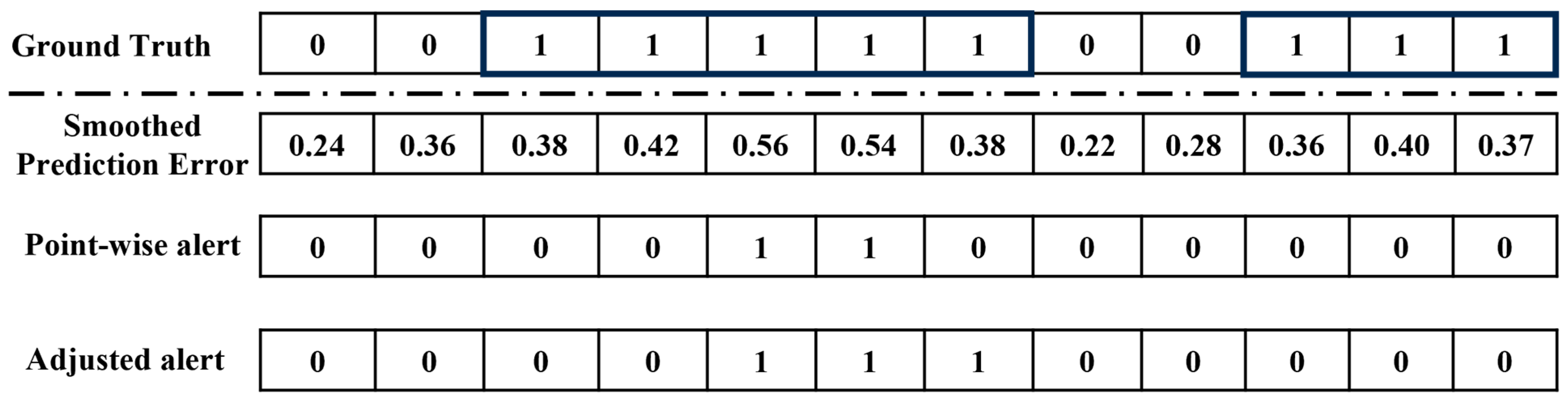
In the context of refrigeration leak detection, a leak is often an anomalous segment. When evaluating similar time-series anomaly detection models, the point adjustment protocols [42] are used; this is because the detection of the anomalous segment is the ultimate objective. For refrigeration leak detection specifically, the time of the leak event plays a crucial role. When calculating precision and recall, it is essential to penalise any delayed discoveries. Therefore, a modified point adjustment protocol is used in this study. All points within the anomalous region after the first successfully detected anomalous point are marked as successfully detected anomalous points, regardless of whether they were accurately captured by the model or not. An example of this protocol is shown in Figure 5, and 0.5 is used as the threshold. The first row represents the ground truth with 12 points, and, within the shaded square, two anomalous segments are highlighted. The second row displays the smoothed prediction error values. The third row presents the point-wise detector results with the specified threshold. Finally, the fourth row showcases the detector results after adjustment.
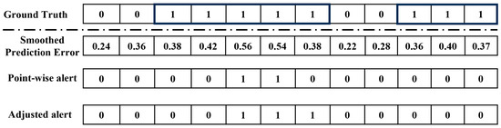
Figure 5.
Point adjustment protocol used in this study.
4. Results and Discussions
In this section, the proposed models to detect catastrophic leaks and slow leaks are evaluated with data obtained from real-world supermarket refrigeration systems. All the algorithms are tested in TensorFlow 2.10.1 with Python 3.10.9on a computer with a GPU of RTX 3070 and CPU 12th Gen Intel(R) i7-12700H 2.30 GHz.
4.1. Catastrophic Leak Detection Results
A single event that occurred in a Canadian supermarket is used to evaluate the proposed model for detecting catastrophic leaks. During this leak event, as depicted in Figure 6, the refrigerant level drops dramatically from 40% to 30% within just a few hours.
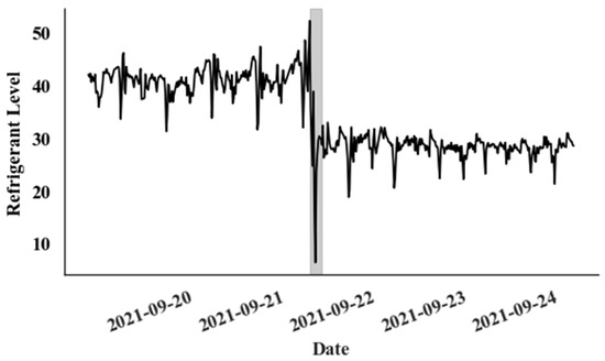
Figure 6.
Catastrophic leak event (Gray colour—Leak period).
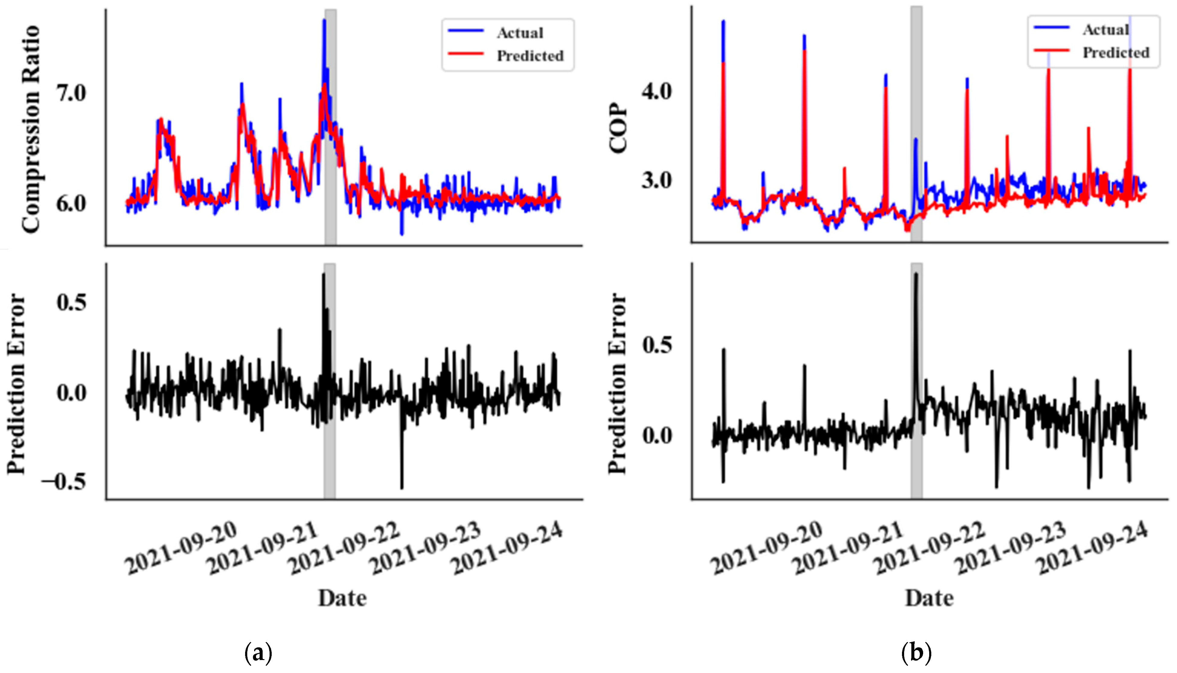
A 15 min sampling interval is used to accurately track the rapid changes in the parameters associated with a catastrophic leak event in Supermarket 1, Rack A. The training data span from 2 August 2021 to 1 September 2021, comprising 2633 data points. The validation set covers the period from 2 September 2021 to 16 September 2021, including 1404 data points, and the test set extends from 17 September 2021 to 16 October 2021, with 2340 data points. The dataset for this particular supermarket is available only from 2 August 2021, and the leak event occurred on 21 September 2021. Therefore, the size of the training set is relatively small. The behaviour of the CatBoost prediction model during the leak event is depicted in Figure 7. Notably, some parameters display a significant change in prediction error, a shift clearly distinct from random noise. But kW values show no significant change from the random noise. The primary distinction between random noise and error fluctuations due to the leak lies in the magnitude and width of the error values.

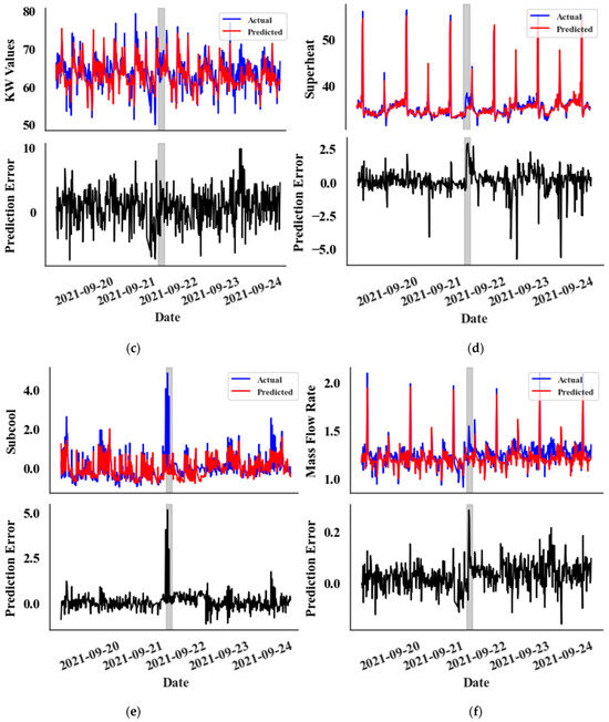
Figure 7.
Prediction vs. Actual data graphs (top) and Prediction Error graphs (bottom) for the test set, featuring the following: (a) Compression Ratio values, (b) COP values, (c) kW Values, (d) Superheat Temperature values, (e) Subcooling temperature values, and (f) Mass Flow Rate values. The leak event is zoomed in for detailed observation.
In the prediction error graphs (lower graphs), an anomaly is noticeable at the very onset of the leak in both the compression ratio (Figure 7a) and subcooling temperature (Figure 7e) metrics. However, the anomaly appears with a slight delay for all other features, except the kW value. Interestingly, the kW graph (Figure 7c) does not exhibit a clear distinction from random noise. This delayed anomaly detection impacts the overall timing of identifying abnormalities.
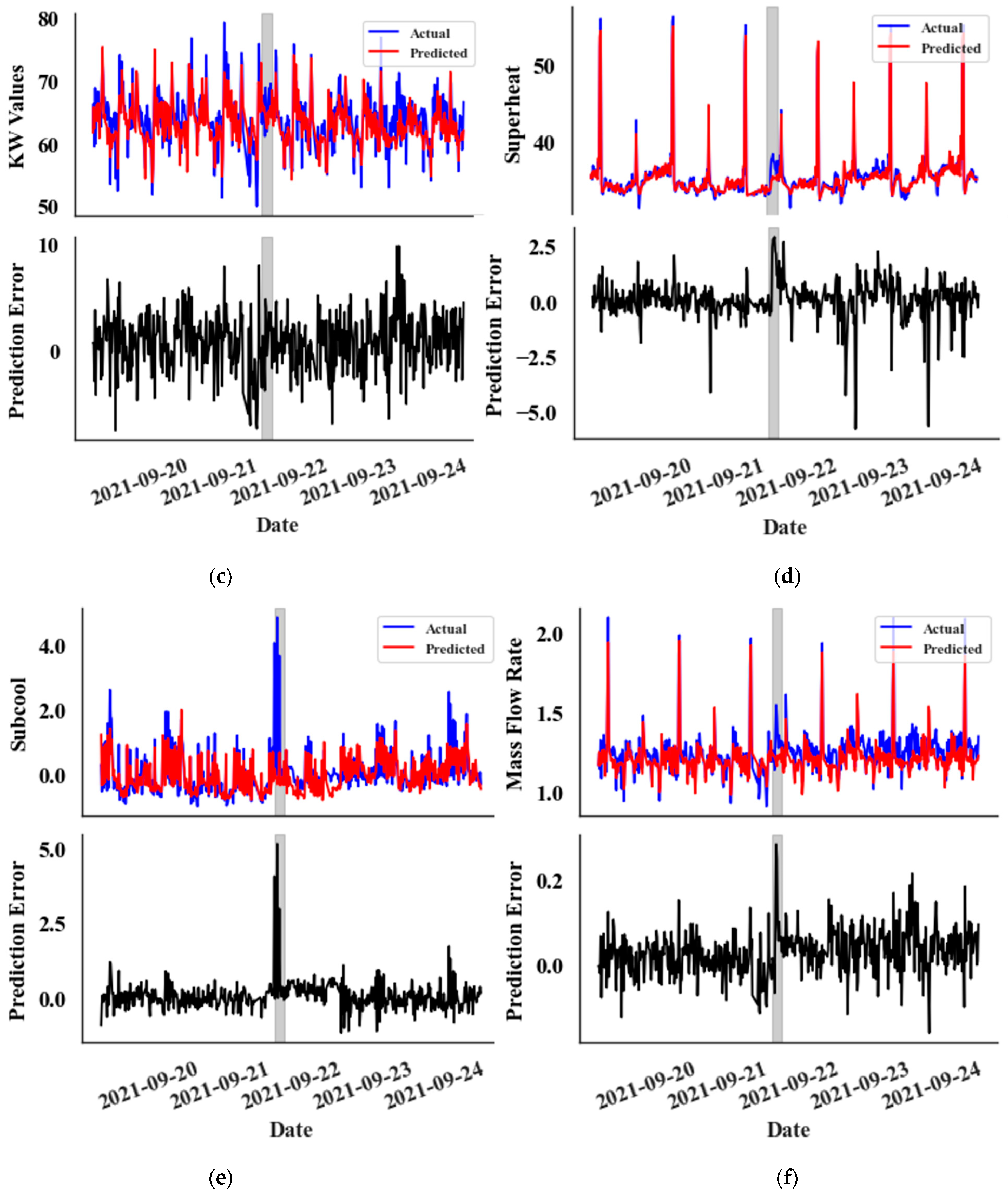
Upon generating predictions from the CatBoost regression model, prediction errors are fed into the nonparametric dynamic thresholding algorithm. This process helps to identify the anomalous points of selected target parameters. Subsequently, these identified anomalous points are superimposed on the graph, representing the refrigerant level values of the receiver. This allows for a clear assessment of the anomaly detection model’s performance (In Supermarket 1, the refrigerant level values at the receiver tank are available. They are not used in any of the modelling. This is used only for the clear visualization of the performance of the anomaly detection model). Figure 8 showcases the efficacy of the non-parametric dynamic thresholding algorithm when it is applied to a dataset containing a leak event before making the point adjustment. The red crosses on the graph signify instances where the model flagged an anomaly.
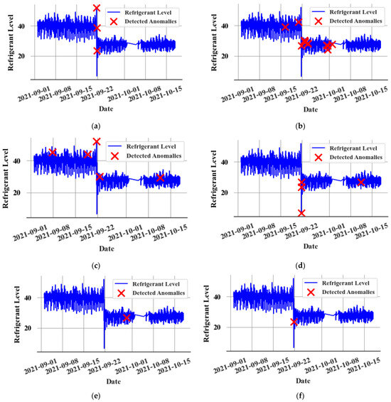
Figure 8.
Anomalies detected using dynamic threshold algorithm for the (a) Subcooling temperature values, (b) Superheat temperature values, (c) Compression Ratio values, (d) COP values, (e) kW values, and (f) Mass flow rate values for a leaking system before point adjustment.
Table 3 summarises the overall performance of the anomaly detection model for each target parameter after making the point adjustment.
Table 3.
Performance of the anomaly detection model.
In addition to promptly detecting a leak, the model should also be capable of minimizing false alarms during normal operations. A challenge of this approach is that the selected target values can be influenced by other faults, potentially complicating the analysis. Table 4 summarises the performance of both the anomaly detection model and the prediction model during a non-leak scenario. Subcooling temperature values are often close to zero, so the calculation of the MAPE value can be erroneous. For the non-leak evaluation, a dataset from the same supermarket (Supermarket 1, Rack A) is obtained for a period when no leak occurred in the store. The composition of the non-leak dataset for this evaluation is as follows: The training set spans from 1 July 2022 to 1 October 2022 and includes 8528 data points. The validation set, containing 1518 data points, extends from 2 October 2022 to 17 October 2022. Finally, the test set covers 17 October 2022 to 18 November 2022, comprising 2928 data points. Unlike the dataset for the leak event, the non-leak dataset is abundant, allowing for a training period that encompasses a full 3 months.
Table 4.
Performance of the prediction model and anomaly detection model for non-leak data.
4.2. Slow Leak Detection Results
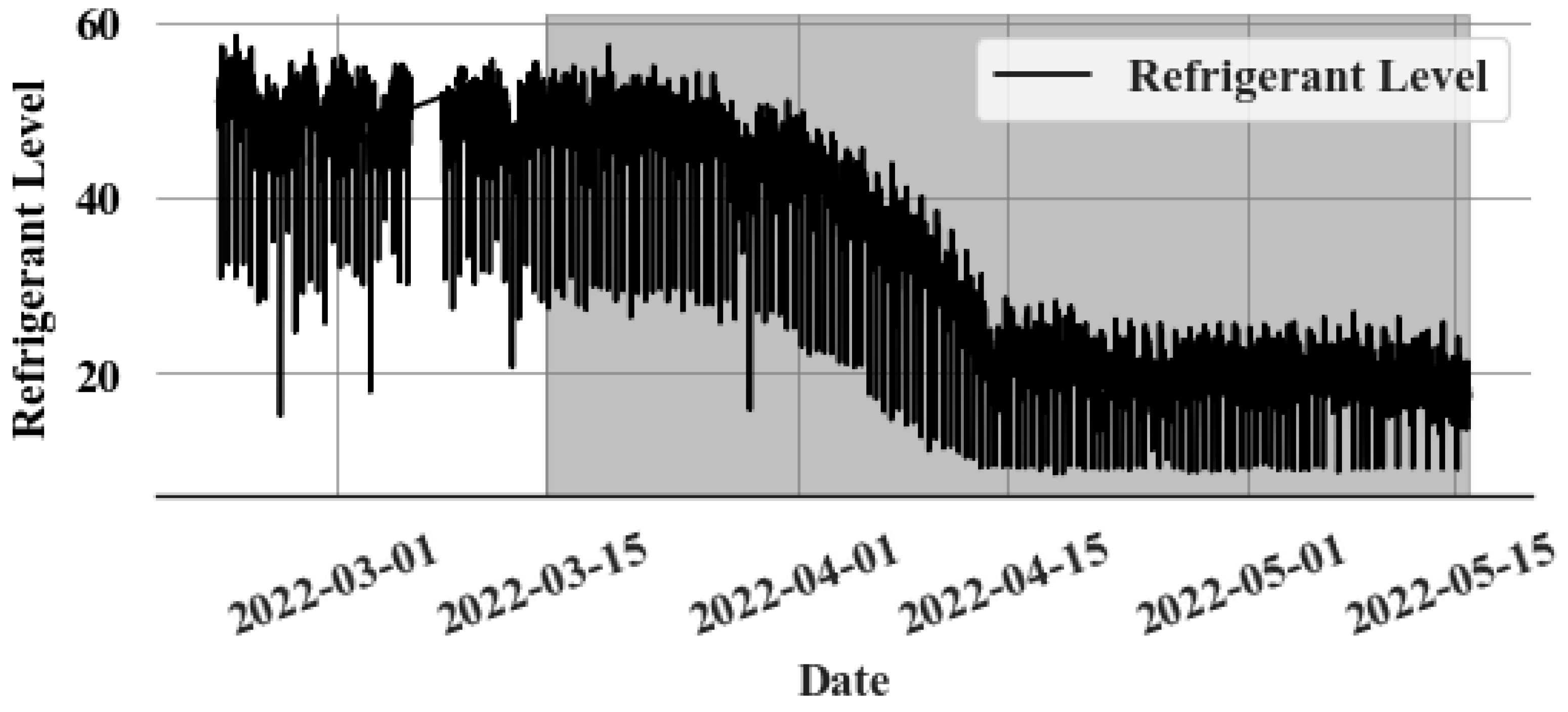
Three slow leak events in three supermarkets are analysed to validate the slow leak detection algorithm. A one-hour sampling window is used for the time series prediction model. Figure 9 shows an example of a slow leak. The leak started on 13 March and slowly expanded until May.

Figure 9.
Slow leak event (Gray colour—Leak period).
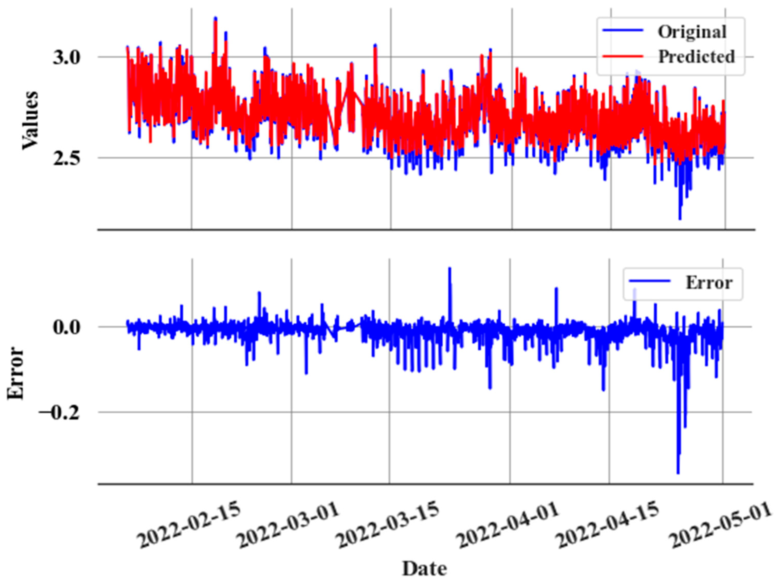
The CatBoost regressor is used to predict COP with data sampled every hour, using the operational data and feature-engineered values as explained in Section 3.3 as input variables. Figure 10 shows how COP exhibits a consistent gradual error at the start of the leak.

Figure 10.
Prediction and actual values during a slow leak (top), and prediction error (e) during a slow leak (bottom).
The cumulative sum of squared errors () is calculated to make the accumulation of gradual errors much more evident. Figure 11 shows the gradient change in the upon the leak’s commencement.
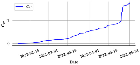
Figure 11.
Cumulative sum of the squared values of the prediction error.
As discussed in the previous section, the bi-weekly rise () of the cumulative sum is calculated from the graph, and the data is resampled on a daily basis by capturing the last value of each day. This graph clearly shows how many errors accumulated during that period. The focus is solely on the gradual, consistent errors (). Therefore, the rapid shifts in the cumulative sum graph are disregarded, with attention paid only to the gradual alterations. This helps to make the algorithm more robust against random noise. Figure 12 depicts the final bi-weekly difference in the cumulative sum graph, excluding rapid increments.
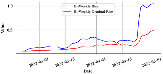
Figure 12.
Gradual cumulative sum change within two weeks, resampled into daily values.
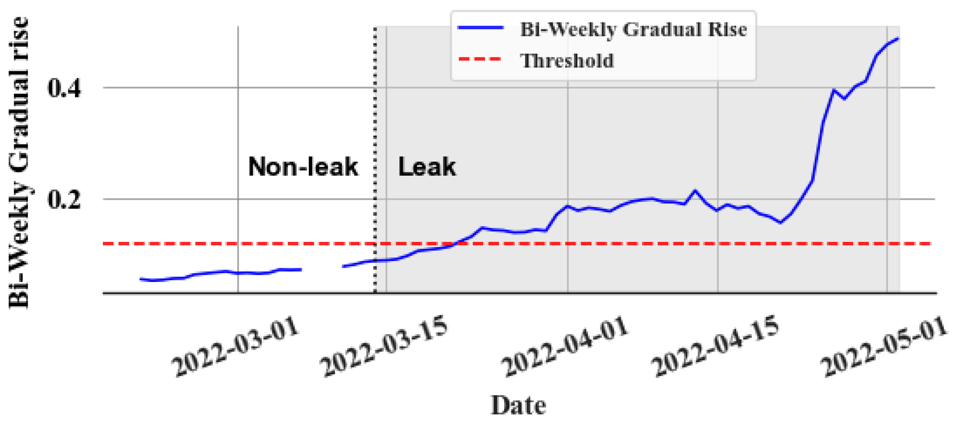
Figure 13 displays the bi-weekly gradual rise () values during a leak event, whereas Figure 14 presents the same during a non-leak event. A clear trend emerges in the values during a leak. Thus, leaks can be identified by establishing an appropriate threshold value. However, the model’s accuracy, as reflected in the mean absolute percentage error (MAPE), along with the goodness of fit indicated by the R2 value, significantly influences the error (e) values. This variation impacts the values, complicating the task of setting a uniform threshold for all stores due to differing accuracies and R2 values at various locations. To overcome this issue, an experimental method is implemented to determine a common ratio value, which can be consistently applied across all stores instead of a variable threshold. The objective of finding the ratio value is to find what multiple of the maximum value of the validation set (i.e., last known non-leak data) should be used. By identifying the optimal ratio, it can be multiplied with the maximum value from each store’s validation set in order to derive a store-specific threshold. In all non-leak cases, this ratio is calculated by dividing the maximum during the non-leak period by the maximum in the validation set. The chosen ratio value should surpass those observed in non-leak events to detect leaks early and effectively reduce false alarms. Experimentally, this value is determined to be 1.8. This approach is based on several key assumptions: First, the data distribution during non-leak periods remains consistent in both validation and test sets. Second, the model retains a high level of predictive accuracy. Lastly, the store’s refrigeration system should be a centralized direct expansion system. Any deviation from these assumptions brings into question the applicability of the 1.8 ratio, necessitating further investigation.
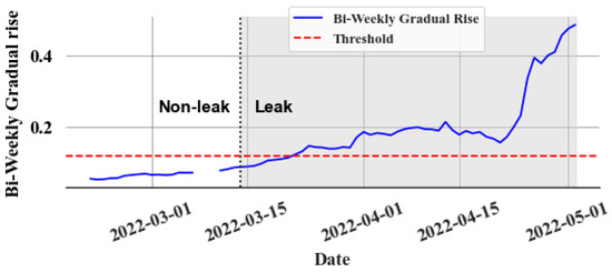
Figure 13.
Bi-weekly gradual rise during a leak event.
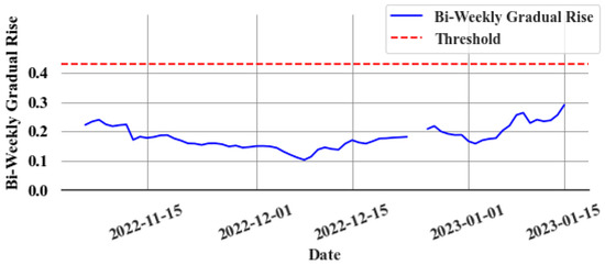
Figure 14.
Bi-weekly gradual rise during a non-leak event.
Figure 13 illustrates how the slow leak detection algorithm performs for the slow leak event depicted in Figure 9. The slow leak event, which commenced on 13 March 2022, continued undetected for over two months. The test set ranged from 1 March 2022 to 1 May 2022 in the experiment conducted. By employing the optimal threshold (0.126), the slow leak is detected within ten days in this example. Figure 14 displays the performance of the slow leak detection algorithm under non-leak conditions. The threshold value applied to the non-leak system is 0.4311. The bi-weekly difference in the gradually increasing cumulative sum does not surpass this threshold value.
The results of the slow leak detection algorithm can be summarised by testing it on three stores. Each performance metric is initially calculated individually for each store. Values are subsequently computed across all the stores in order to provide a sense of the algorithm’s overall efficacy. The same parameters are used on the healthy data for each store to evaluate the model’s performance during the non-leak period. Table 5 shows the information about the datasets used to evaluate slow leak detection, and Table 6 shows the average performance of the slow leak detection model considering all three datasets. Similarly, Table 7 and Table 8 show the datasets used to evaluate the model’s performance during the non-leak period and their performance. In Supermarket 3, Rack B, there was insufficient data with normal non-leak behaviour to train a model.
Table 5.
Description of the datasets with slow leak events that are used to evaluate the slow leak detection model.
Table 6.
Performance of the slow leak detection model.
Table 7.
Description of the datasets with non-leak data used to evaluate the prediction model.
Table 8.
Performance of the prediction model for non-leak data.
The exact names of supermarkets are not revealed; instead, code names such as Supermarket1 and Supermarket2 are used in this study.
5. Conclusions
This paper introduces a novel framework for detecting both catastrophic and slow leaks, as validated using real-world data from supermarket refrigeration systems in Canada. The main innovations of this research are as follows: First, the solution demonstrates exceptional effectiveness in detecting both slow and catastrophic leaks. Second, it operates independently of the refrigerant level sensor in the receiver tank, a common dependency in many other solutions. Third, the integration of false alarm mitigation techniques ensures a robust performance, even during transitions in control modes. In catastrophic leak scenarios, all targeted features, except for the kW values of the system rack, exhibit a sudden change in prediction error, clearly distinguishing them from random noise. For slow leaks, only the calculated coefficient of performance (COP) values display a gradual yet consistent prediction error, resulting from disrupted relationships between the input features. The proposed solution is capable of detecting a slow leak within an average of five days from its onset. In contrast, it typically takes technicians months to notice most refrigerant leaks. The dataset used for evaluation includes one catastrophic leak event and three slow leak events from different stores. Each leak detection algorithm’s performance was assessed based on its ability to reliably identify leaks with a minimal rate of false alarms. Future research will explore a deep learning-based approach in order to better capture complex non-linear relationships and enhance the anomaly detection strategy, aiming to improve accuracy and further reduce false alarms.
Author Contributions
Methodology, R.W., H.N. and C.Z.; Validation, R.W.; Formal analysis, R.W.; Investigation, R.W., H.N. and C.Z.; Writing—original draft, R.W.; Writing—review & editing, H.N., J.S. and A.S.; Supervision, J.S. and A.S.; Project administration, C.Z.; Funding acquisition, C.Z. and A.S. All authors have read and agreed to the published version of the manuscript.
Funding
The proposed research was funded by Mitacs Accelerate Grant and the Neelands Group.
Data Availability Statement
The raw data supporting the conclusions of this article will be made available by the authors on request.
Conflicts of Interest
H.N. and C.Z. were employed by Neelands Group Ltd. The remaining authors declare that the research was conducted in the absence of any commercial or financial relationships that could be construed as a potential conflict of interest. The authors declare that this study received funding from Neelands Group. The funder was not involved in the study design, collection, analysis, interpretation of data, the writing of this article or the decision to submit it for publication.
References
- Natural Resources Canada. Heads Up: Building Energy Efficiency–Volume 2, Issue 3 (March). 3 July 2018. Available online: https://natural-resources.canada.ca/energy-efficiency/buildings/energy-management-resources-buildings/heads-building-energy-efficiency-newsletter/heads-building-energy-efficiency-volume-2-issue-3-march/17356 (accessed on 25 July 2023).
- Natural Resources Canada. Survey of Commercial and Institutional Energy Use: Buildings 2009: Detailed Statistical Report, December, 2012; Natural Resources Canada: Ottawa, ON, Canada, 2012. [Google Scholar]
- EnergyStar. Energy Star Building Manual—Facility Type: Supermarkets and Grocery Stores. 2008. Available online: https://www.energystar.gov/sites/default/files/buildings/tools/EPA_BUM_CH11_Supermarkets.pdf (accessed on 26 July 2023).
- Behfar, A.; Yuill, D.; Yu, Y. Supermarket system characteristics and operating faults (RP-1615). Sci. Technol. Built Environ. 2018, 24, 1104–1113. [Google Scholar] [CrossRef]
- Walker, D.H. Development and demonstration of an advanced supermarket refrigeration/HVAC system. In Final Analysis Report; ORNL Subcontract Number 62X-SX363C; Foster-Miller, Inc.: Waltham, MA, USA, 2001; Volume 2451. [Google Scholar]
- Francis, C.; Maidment, G.; Davies, G. An investigation of refrigerant leakage in commercial refrigeration. Int. J. Refrig. 2017, 74, 12–21. [Google Scholar] [CrossRef]
- Cowan, D.; Gartshore, J.; Chaer, I.; Francis, C.; Maidment, G. REAL Zero–Reducing Refrigerant Emissions & Leakage-Feedback from the IOR Project. 2011. Available online: https://openresearch.lsbu.ac.uk/download/341ef7aa04d2bc160c57e2dd1ec55e8f4883eb20572c34090169160654631e8a/393472/IOR_ReducingRefrigerantEmissions.pdf (accessed on 17 August 2023).
- Heath, E.A. Amendment to the Montreal protocol on substances that deplete the ozone layer (Kigali amendment). Int. Leg. Mater. 2017, 56, 193–205. [Google Scholar] [CrossRef]
- Regulation (EU) No 517/2014 of the European Parliament and of the Council of 16 April 2014 on Fluorinated Greenhouse Gases and Repealing Regulation (EC) No 842/2006 Text with EEA Relevance. 2014; Volume 150. Available online: http://data.europa.eu/eli/reg/2014/517/oj/eng (accessed on 25 July 2023).
- Protection of Stratospheric Ozone: Revisions to the Refrigerant Management Program’s Extension to Substitutes. Federal Register. 11 March 2020. Available online: https://www.federalregister.gov/documents/2020/03/11/2020-04773/protection-of-stratospheric-ozone-revisions-to-the-refrigerant-management-programs-extension-to (accessed on 25 July 2023).
- Lasi, H.; Fettke, P.; Kemper, H.-G.; Feld, T.; Hoffmann, M. Industry 4.0. Bus. Inf. Syst. Eng. 2014, 6, 239–242. [Google Scholar] [CrossRef]
- Mirnaghi, M.S.; Haghighat, F. Fault detection and diagnosis of large-scale HVAC systems in buildings using data-driven methods: A comprehensive review. Energy Build. 2020, 229, 110492. [Google Scholar] [CrossRef]
- Verbert, K.; Babuška, R.; De Schutter, B. Combining knowledge and historical data for system-level fault diagnosis of HVAC systems. Eng. Appl. Artif. Intell. 2017, 59, 260–273. [Google Scholar] [CrossRef]
- Shen, C.; Zhang, H.; Meng, S.; Li, C. Augmented data driven self-attention deep learning method for imbalanced fault diagnosis of the HVAC chiller. Eng. Appl. Artif. Intell. 2023, 117, 105540. [Google Scholar] [CrossRef]
- Behfar, A.; Yuill, D.; Yu, Y. Automated fault detection and diagnosis methods for supermarket equipment (RP-1615). Sci. Technol. Built Environ. 2017, 23, 1253–1266. [Google Scholar] [CrossRef]
- Srinivasan, S.; Vasan, A.; Sarangan, V.; Sivasubramaniam, A. Bugs in the Freezer: Detecting Faults in Supermarket Refrigeration Systems Using Energy Signals. In Proceedings of the 2015 ACM Sixth International Conference on Future Energy Systems, Bangalore, India, 14–17 July 2015; ACM: New York, NY, USA, 2015; pp. 101–110. [Google Scholar] [CrossRef]
- Assawamartbunlue, K.; Brandemuehl, M. Refrigerant Leakage Detection and Diagnosis for a Distributed Refrigeration System. HVACR Res. 2006, 12, 389–405. [Google Scholar] [CrossRef]
- Behfar, A.; Yuill, D.; Yu, Y. Automated fault detection and diagnosis for supermarkets–method selection, replication, and applicability. Energy Build. 2019, 198, 520–527. [Google Scholar] [CrossRef]
- Sun, J.; Im, P.; Bae, Y.; Munk, J.; Kuruganti, T.; Fricke, B. Fault detection of low global warming potential refrigerant supermarket refrigeration system: Experimental investigation. Case Stud. Therm. Eng. 2021, 26, 101200. [Google Scholar] [CrossRef]
- Wichman, A.; Braun, J. Fault Detection and Diagnostics for Commercial Coolers and Freezers. HVACR Res. 2009, 15, 77–99. [Google Scholar] [CrossRef]
- Mavromatidis, G.; Acha, S.; Shah, N. Diagnostic tools of energy performance for supermarkets using Artificial Neural Network algorithms. Energy Build. 2013, 62, 304–314. [Google Scholar] [CrossRef]
- Fisera, R.; Stluka, P. Performance Monitoring of the Refrigeration System with Minimum Set of Sensors. Int. J. Electr. Comput. Eng. 2012, 6, 637–642. [Google Scholar]
- Tassou, S.A.; Grace, I.N. Fault diagnosis and refrigerant leak detection in vapour compression refrigeration systems. Int. J. Refrig. 2005, 28, 680–688. [Google Scholar] [CrossRef]
- Han, H.; Cao, Z.; Gu, B.; Ren, N. PCA-SVM-Based Automated Fault Detection and Diagnosis (AFDD) for Vapor-Compression Refrigeration Systems. HVACR Res. 2010, 16, 295–313. [Google Scholar] [CrossRef]
- Yang, Z.; Rasmussen, K.B.; Kieu, A.T.; Izadi-Zamanabadi, R. Fault Detection and Isolation for a Supermarket Refrigeration System–Part One: Kalman-Filter-Based Methods. IFAC Proc. Vol. 2011, 44, 13233–13238. [Google Scholar] [CrossRef]
- Yang, Z.; Rasmussen, K.B.; Kieu, A.T.; Izadi-Zamanabadi, R. Fault Detection and Isolation for a Supermarket Refrigeration System–Part Two: Unknown-Input-Observer Method and Its Extension. IFAC Proc. Vol. 2011, 44, 4238–4243. [Google Scholar] [CrossRef]
- Chen, B.; Braun, J.E. Simple rule-based methods for fault detection and diagnostics applied to packaged air conditioners/Discussion. ASHRAE Trans. 2001, 107, 847. [Google Scholar]
- Mota-Babiloni, A.; Navarro-Esbrí, J.; Barragán-Cervera, Á.; Molés, F.; Peris, B.; Verdú, G. Commercial refrigeration–An overview of current status. Int. J. Refrig. 2015, 57, 186–196. [Google Scholar] [CrossRef]
- Evans, J.A.; Foster, A.M. (Eds.) Sustainable Retail Refrigeration; Wiley Blackwell: Chichester, UK; Hoboken, NJ, USA, 2015. [Google Scholar]
- ICF Consulting. Revised Draft Analysis of U.S. Commercial Supermarket Refrigeration Systems; US Environmental Protection Agency EPA: Washington, DC, USA, 2005.
- Prokhorenkova, L.; Gusev, G.; Vorobev, A.; Dorogush, A.V.; Gulin, A. CatBoost: Unbiased boosting with categorical features. Adv. Neural Inf. Process. Syst. 2018, 31, 6638–6648. [Google Scholar]
- Jabeur, S.B.; Gharib, C.; Mefteh-Wali, S.; Arfi, W.B. CatBoost model and artificial intelligence techniques for corporate failure prediction. Technol. Forecast. Soc. Chang. 2021, 166, 120658. [Google Scholar] [CrossRef]
- Fan, J.; Wang, X.; Zhang, F.; Ma, X.; Wu, L. Predicting daily diffuse horizontal solar radiation in various climatic regions of China using support vector machine and tree-based soft computing models with local and extrinsic climatic data. J. Clean. Prod. 2020, 248, 119264. [Google Scholar] [CrossRef]
- Diao, L.; Niu, D.; Zang, Z.; Chen, C. Short-term Weather Forecast Based on Wavelet Denoising and Catboost. In Proceedings of the 2019 Chinese Control Conference (CCC), Guangzhou, China, 27–30 July 2019; pp. 3760–3764. [Google Scholar] [CrossRef]
- Hancock, J.T.; Khoshgoftaar, T.M. CatBoost for big data: An interdisciplinary review. J. Big Data 2020, 7, 94. [Google Scholar] [CrossRef] [PubMed]
- Kohavi, R. Bottom-up induction of oblivious read-once decision graphs. In Machine Learning: ECML-94; Bergadano, F., De Raedt, L., Eds.; Lecture Notes in Computer Science; Springer: Berlin/Heidelberg, Germany, 1994; Volume 784, pp. 154–169. [Google Scholar] [CrossRef]
- Grace, I.N.; Datta, D.; Tassou, S.A. Sensitivity of refrigeration system performance to charge levels and parameters for on-line leak detection. Appl. Therm. Eng. 2005, 25, 557–566. [Google Scholar] [CrossRef]
- Zeng, Y.; Chen, H.; Xu, C.; Cheng, Y.; Gong, Q. A hybrid deep forest approach for outlier detection and fault diagnosis of variable refrigerant flow system. Int. J. Refrig. 2020, 120, 104–118. [Google Scholar] [CrossRef]
- Bell, I.H.; Wronski, J.; Quoilin, S.; Lemort, V. Pure and Pseudo-pure Fluid Thermophysical Property Evaluation and the Open-Source Thermophysical Property Library CoolProp. Ind. Eng. Chem. Res. 2014, 53, 2498–2508. [Google Scholar] [CrossRef] [PubMed]
- Cho, H.; Ryu, C.; Kim, Y.; Kim, H.Y. Effects of refrigerant charge amount on the performance of a transcritical CO2 heat pump. Int. J. Refrig. 2005, 28, 1266–1273. [Google Scholar] [CrossRef]
- Hundman, K.; Constantinou, V.; Laporte, C.; Colwell, I.; Soderstrom, T. Detecting Spacecraft Anomalies Using LSTMs and Nonparametric Dynamic Thresholding. In Proceedings of the 24th ACM SIGKDD International Conference on Knowledge Discovery & Data Mining, London, UK, 19–23 August 2018; ACM: New York, NY, USA, 2018; pp. 387–395. [Google Scholar] [CrossRef]
- Xu, H.; Chen, W.; Zhao, N.; Li, Z.; Bu, J.; Li, Z.; Liu, Y.; Zhao, Y.; Pei, D.; Feng, Y.; et al. Unsupervised Anomaly Detection via Variational Auto-Encoder for Seasonal KPIs in Web Applications. In Proceedings of the 2018 World Wide Web Conference on World Wide Web-WWW’18, Lyon, France, 23–27 April 2018; ACM Press: New York, NY, USA, 2018; pp. 187–196. [Google Scholar] [CrossRef]


Disclaimer/Publisher’s Note: The statements, opinions and data contained in all publications are solely those of the individual author(s) and contributor(s) and not of MDPI and/or the editor(s). MDPI and/or the editor(s) disclaim responsibility for any injury to people or property resulting from any ideas, methods, instructions or products referred to in the content. |
© 2024 by the authors. Licensee MDPI, Basel, Switzerland. This article is an open access article distributed under the terms and conditions of the Creative Commons Attribution (CC BY) license (https://creativecommons.org/licenses/by/4.0/).