On SINDy Approach to Measure-Based Detection of Nonlinear Energy Flows in Power Grids with High Penetration Inverter-Based Renewables

Abstract

The complexity of modern power grids, caused by integrating renewable energy sources, especially inverter-based resources, presents a significant challenge to grid operation and planning, since linear models are unable to capture the complex nonlinear dynamics of power systems with coupled muti-scale dynamics, and it necessitate an alternative approach utilizing more advanced and data-driven algorithms to improve modeling accuracy and system optimization. This study employs the sparse identification of nonlinear dynamics method by leveraging compressed sensing and sparse modeling principles, offering robustness and the potential for generalization, allowing for identifying key dynamical features with relatively few measurements, and providing deeper theoretical understanding in the field of power system analysis. Taking advantage of the this method in recognizing the active terms (first and high order) in the system’s governing equation, this paper also introduces the novel Volterra-based nonlinearity index to characterize system-level nonlinearity. The distinction of dynamics into first-order linearizable terms, second-order nonlinear dynamics, and third-order noise is adopted to clearly show the intricacy of power systems. The findings demonstrate a fundamental shift in system dynamics as power sources transit to inverter-based resources, revealing system-level (second-order) nonlinearity compared to module-level (first order) nonlinearity in conventional synchronous generators. The proposed index quantifies nonlinear-to-linear relationships, enriching our comprehension of power system behavior and offering a tool for distinguishing between different nonlinearities and visualizing their distinct patterns through the profile of the proposed index.

1. Introduction

While machine learning algorithms and artificial intelligence have improved system analysis by overcoming the limitations of conventional models in capturing the intricate nonlinear dynamics of power systems, the incorporation of inverter-based energy resources (IBRs) with interconnected multi-scale dynamics requires a thorough analysis and characterization of the nonlinearity of the system [1,2,3,4]. The systemic nonlinearity conundrum is a central focus in power system operation due to the intricate dynamics within modern power grids [5]. As these grids increasingly incorporate diverse energy sources, including IBRs, conventional linear models fail to capture the complex web of nonlinear interactions, feedback loops, and emergent behaviors [6]. The recognition and comprehensive examination of system-level (second order) nonlinearity are paramount for safeguarding the resilience, stability, and efficiency of contemporary electrical grids.

Recent studies emphasized the transformative impact of IBR integration in power system dynamics. The work by Mishra et al. (2022) uncover the intrinsic nonlinearities within conventional power grids, highlighting the challenge of maintaining stability amid dynamic interactions among synchronous generators and intricate load profiles [7]. Ekomwenrenren et al. (2021) empirically demonstrate deviations from conventional linearized frequency control in IBR grids, revealing nuanced nonlinear frequency responses unique to these systems [8]. Orihara et al. (2021) delve into the pivotal dynamics of virtual inertia in IBR grids, offering insights into nonlinear control mechanisms [9]. Keyon et al. (2020) examine the impact of varying IBR penetration levels on power system dynamics, illustrating the transition from first-order to high-order behavior [10].

Understanding the distinctions between synchronous generators (SGs) and the interactions within systems that combine SGs and IBRs or rely exclusively on IBRs is vital for system operators [11]. The most significant impacts in power system analysis and management materialize in real-time operations, where precise mathematical system dynamics models are often unattainable [12].

Measurement-based methodologies, rooted in the observed data and supported by advanced monitoring technologies and data analytics, provide a solution for real-time decision support. These techniques empower grid operators to make informed decisions that ensure the continuity of electrical power systems’ stability and the reliability of evolving energy landscapes characterized by nonlinear dynamics and grid architectures [13].

There is potential for innovative approaches that extend and refine the SINDy paradigm, making it applicable and relevant across diverse domains [14,15]. Integrating sparsity methods in analyzing dynamical systems is a significant advancement, employing compressed sensing and sparse regression techniques to identify concise and accurate models representing the underlying nonlinear dynamics [16]. SINDy is a measure-based method specifically designed to discover governing equations or mathematical models from observed data.

The development and application of advanced modeling techniques, such as SINDy, are essential in understanding modern power systems’ higher-order dynamics and nuanced interdependencies [17]. Since its inception in 2016, the SINDy algorithm has been extensively adopted for model identification in diverse fields. It has demonstrated impressive efficacy by explicitly recognizing governing equations through sparse regression techniques, resulting in interpretable models that adeptly handle complexity. The development and adaptation of SINDy techniques provide the following benefits:

• Provide a novel avenue for understanding complex systems;
• Enrich our understanding of fundamental principles;
• Pave the way for groundbreaking applications and insight in various fields of study [18,19].

While the SINDy algorithm has found applications in various disciplines, its utilization in power system analysis has been limited, with only a handful of studies exploring its potential in this domain [20,21,22,23]. Notably, these investigations have predominantly focused on analyzing the broader power system and have primarily relied on first-order system models, as exemplified in a 2020 paper on power system applications [20].

This paper represents a significant contribution to the field, as it utilizes the SINDy method in power systems, investigating a diverse set of conditions, encompassing both abrupt changes (faults) and gradual changes (load variations). This approach ensures robustness and the potential for generalization, and it enables the identification of key dynamical features with relatively few measurements, enhancing our theoretical understanding of power system analysis. Leveraging this method to distinguish active terms, of both first and high order, in the system’s governing equation, the study introduces the Volterra-based nonlinearity index (VNI). This index characterizes system-level nonlinearity by distinguishing between first-order linearizable terms, second-order nonlinear dynamics, and third-order noise, providing a comprehensive understanding of power systems’ intricacies. The results show a fundamental shift in system dynamics as power sources transition to IBRs, revealing system-level nonlinearity compared to module-level nonlinearity in conventional generators. The proposed index quantifies nonlinear-to-linear relationships and enriches our comprehension of power system behavior, offering a valuable tool for distinguishing between different nonlinearities and visualizing their distinct patterns through the index’s profile.

The introduction of higher-order polynomial function libraries to model IBR integration represents a significant departure from traditional modeling approaches, reflecting the evolving needs of power grid analyses as renewable energies dominate. The findings pave the way for a better understanding of the intricacies of power systems and offer practical solutions for building more resilient and efficient grids.

The subsequent sections of this manuscript are organized as follows: Section 2 describes the developed SINDy method for power systems. Section 3 demonstrates the conducted study and the respective results followed by the introduction of the proposed index for system nonlinearity. The final segment comprises the concluding remarks, emphasizing the results’ significance and suggesting potential research directions for future studies.

2. SINDy Algorithm

In this section, we will delve into the mechanics of the SINDy framework, exploring its fundamental principles and methodologies to develop an algorithm that is suitable for power system analysis. We will begin by examining how SINDy leverages sparsity methods, compressed sensing, and sparse regression techniques to identify concise and accurate models for complex dynamical systems. We will dissect the critical steps of the SINDy approach, from data collection and constructing a library of candidate functions to sparse regression and model construction. Additionally, we will highlight the significance of sparsity in simplifying system dynamics and improving interpretability. Finally, we will introduce a three-section data analysis structure, which extends SINDy’s capabilities for enhanced data-driven research across diverse domains.

Analyses of nonlinear dynamics in electric power systems typically rely on a set of first-order ordinary differential equations that accommodate various scales, expressed as [24]:

$$\frac{du}{dt}=F\left(u,\beta ,\mathsf{\gamma }\right)$$

(1)

In this equation, $\beta$ and $\gamma$ denote two parameters representing independent inputs steering the system. These inputs encompass rapidly changing factors, such as active IBRs, and slowly changing elements, such as passive loads [24,25]. With a slight modification of the function F to incorporate passive loads ($\gamma$), the equation aligns with those characterizing general dissipative energy systems:

$$\frac{du}{dt}=F\left(u,\beta \right)$$

(2)

Here, u signifies the system states typically observable, and $\beta$ denotes the inputs actively driving the system [25].

Considering the voltage as the observable variable, the dynamics of a power system can be described using the following general form [26]:

$$\frac{dv\left(t\right)}{dt}=f\left(v\left(t\right)\right),$$

(3)

where $v\left(t\right)\in R^n$ represents the system’s voltage at time $t,$ and $f\left(v\right(t\left)\right)$ encompasses the dynamic constraints governing the system’s equations, including parameters, time dependence, and external forcing.

Integrating sparsity methods in analyzing dynamical systems has emerged as a significant advancement, employing compressed sensing and sparse regression techniques to identify concise and accurate models representing the underlying nonlinear dynamics [19]. SINDy is a measure-based method specifically designed to discover governing equations or mathematical models from observed data. The SINDy approach focuses on dynamical systems described using the Equation (3).

Leveraging recent progress in compressed sensing and sparse regression, the sparsity perspective enables the identification of the nonzero terms in $f$ without computationally demanding brute-force searches. 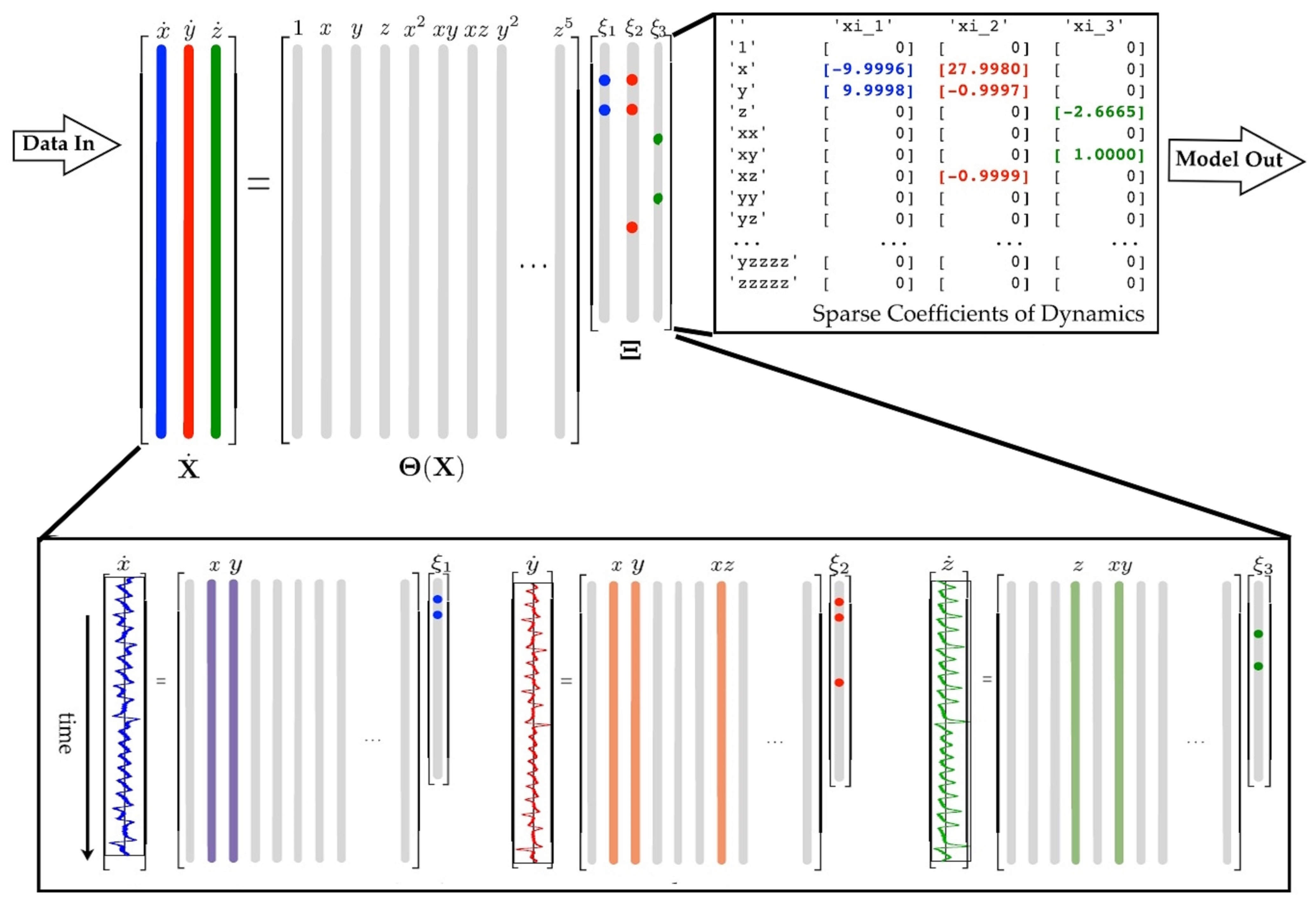Convex methods that scale well with Moore’s law allow for identifying sparse solutions with high probability, striking a balance between model complexity and accuracy, thereby avoiding overfitting the model to the available data [18]. An example case is illustrated in Figure 1 to demonstrate SINDy’s algorithm [7].

To determine the function $f$ from the available data, a time history of the system’s state, denoted as $v\left(t\right)$, is collected. The derivative of $v\left(t\right)$, denoted as $\dot{v}\left(t\right)$, is directly or numerically approximated. The data are sampled at various time instances, ${\{t}_1,t_2,\dots ,t_m$} and organized into $V$ and $\dot{V}$ matrices. The matrix $V$ is constructed as follows:

$$V={\left[\begin{array}{c}|\\ v\left(t_1\right),\\ |\end{array}\begin{array}{c}|\\ v\left(t_2\right)\\ |\end{array},\dots ,\begin{array}{c}|\\ v\left(t_m\right)\\ |\end{array}\right]}^T$$

(4)

and the matrix $\dot{V}$ is constructed as follows:

$$\dot{V}={\left[\begin{array}{c}|\\ \dot{v}\left(t_1\right)\\ |\end{array},\begin{array}{c}|\\ \dot{v}\left(t_2\right)\\ |\end{array},\dots ,\begin{array}{c}|\\ \dot{v}\left(t_m\right)\\ |\end{array}\right]}^T$$

(5)

The next step in the SINDy approach involves defining a library of candidate functions, denoted as $\Theta \left(V\right)$, where $V$ is the data matrix that contains the observed data points of the system variables [7]. The library is constructed by carefully selecting relevant nonlinear functions based on prior knowledge and theoretical considerations. These functions can include polynomials, trigonometric functions, exponentials, logarithmic functions, and other suitable nonlinear expressions [7].

$$\Theta \left(V\right)=\left[1,V,V^2,V^3,\dots ,cos\left(V\right),sin\left(V\right),\dots \right]$$

(6)

Higher-order polynomials are denoted as $V^2$, $V^3$, and so on. Each column in the $\Theta \left(V\right)$ matrix represents a candidate function for the right-hand side of the dynamical equation [7].

Assuming that only a few of these nonlinearities are active in each row of $f$, a sparse regression problem is formulated to determine the sparse vectors of coefficients,

$$\Xi =\left[\begin{array}{c}|\\ {\xi }_1\\ |\end{array},\begin{array}{c}|\\ {\xi }_2\\ |\end{array},\dots ,\begin{array}{c}|\\ {\xi }_n\\ |\end{array}\right]$$

(7)

which indicate the active nonlinearities. Mathematically, this can be expressed as follows:

$$\dot{V}=\Theta \left(V\right)\Xi .$$

(8)

Each column, ${\xi }_k$, of the $\Xi$ matrix corresponds to a sparse vector of coefficients that determines the active terms in the right-hand side of one of the row equations, $v_k=f\left(v\right)$ [7,19].

Given the data matrix $V$ and the library of candidate functions $\Theta \left(V\right)$, SINDy formulates the sparse regression problem as follows:

$$minimize{\left||\dot{V}-\Theta \left(V\right)\Xi |\right|}_2+\lambda {\left|\left|\Xi \right|\right|}_1$$

(9)

where $\Xi$ is the sparse vector of coefficients representing the importance or relevance of each term in the library, ${\left|\left|.\right|\right|}_2$ denotes the L2 norm, ${\left|\left|.\right|\right|}_1$ represents the L1 norm, and $\lambda$ is a regularization parameter that controls the trade-off between data fidelity and sparsity. The first term in Equation (9) ensures that the model predictions, obtained by multiplying $\Theta \left(V\right)$ with $\Xi$, are close to the observed data, while the second term encourages a sparse solution by promoting a minimal number of nonzero coefficients [7].

The sparsity principle is central to this approach, as it seeks to select a subset of functions from the candidate library that is most relevant to the system’s dynamics. By incorporating regularization techniques, such as L1 regularization (or the Lasso), the model achieves sparsity by encouraging the coefficients of irrelevant terms to be zero, thereby emphasizing the significant functions while minimizing the overall number of terms [18]. This strategy simplifies the representation of system dynamics, leading to improved interpretability and a more concise model.

Once the Ξ matrix is determined, a model for each row equation can be constructed using the library of candidate functions and the corresponding sparse coefficients. Specifically, the kth row equation, $v_k=f\left(v\right)$, can be expressed as follows:

$$v_k=\Theta \left(v\right){\xi }_k,$$

(10)

where $\Theta \left(v\right)$ is a vector of symbolic functions of the elements of v. It is important to note that $\Theta \left(v\right)$ differs from $\Theta \left(V\right)$ in that it represents symbolic functions of the state variables, unlike $\Theta \left(V\right)$, which represents a data matrix. Consequently, the overall representation of the system dynamics can be written as follows:

$$\dot{v}=f\left(v\right)={\Xi }^T\Theta \left(v\right)$$

(11)

Each column requires a separate optimization procedure to determine the sparse vector of coefficients, ${\xi }_k$, for the corresponding row equation. It is also possible to normalize the columns of $\Theta \left(V\right)$, particularly when the entries of $V$ are small.

SINDy has been extensively studied and validated in various scientific domains, showcasing its effectiveness in uncovering governing equations from data. However, the method has limitations. SINDy is sensitive to noise and requires careful model selection to balance sparsity and accuracy [27]. Its application to densely coupled dynamics poses challenges as disentangling individual contributions becomes difficult [28]. Furthermore, while SINDy captures dynamics from data, it does not explicitly incorporate physical constraints, necessitating additional techniques or prior knowledge incorporation to ensure compliance with fundamental principles [7,27]. Awareness of these limitations is essential for the effective and informed utilization of the SINDy method.

The proposed three-section data analysis structure represents a notable evolution in data analysis, particularly within the SINDy framework. This innovative structure introduces a novel third section that extends the conventional SINDy methodology, providing new avenues for enhanced data analysis. The initial two sections focus on identifying linearizable and nonlinear dynamics within the system [29]. The addition of the third section substantially enhances the overall data analysis process by categorizing and managing negligible data, often regarded as noise, which significantly improves the precision and accuracy of system modeling. This comprehensive approach enables a more profound understanding of intricate nonlinear behaviors, benefiting applications across diverse domains. The inclusion of the third section underscores the adaptability and versatility of the SINDy methodology, allowing for a more nuanced examination of complex system dynamics, which is a critical component of contemporary data-driven research.

The first section of the proposed data analysis framework plays a fundamental role in identifying and characterizing first-order impacts within the system. Its unique focus lies in evaluating the nonlinearities across nodes, with a particular emphasis on those that are trivial or readily linearizable. This systematic approach dissects the system dynamics to isolate elements that exhibit straightforward and manageable nonlinearities amenable to linear approximations. This categorization enhances the precision and tractability of the data analysis process, providing insights into complex system behaviors encompassing both linear and nonlinear components, particularly in applications spanning diverse domains, including power systems.

The second section within the outlined data analysis structure takes a central role in the comprehensive examination of system dynamics. It is dedicated to discerning and categorizing true nonlinearity, which differs significantly from the more straightforward and readily linearizable elements identified in the first section. True nonlinearity represents intricate and nontrivial characteristics that defy simple linearization, delving deep into complex system behaviors. Focusing on these inherently nonlinear dynamics offers profound insights into the intricate interdependencies and feedback loops characterizing real-world systems, transcending linear approximation constraints. This in-depth analysis is pivotal for understanding nonlinearity’s nuances across various domains, providing a foundation for a richer comprehension of system dynamics, particularly in the context of power systems and beyond.

The third section within the data analysis structure plays a role in isolating and addressing components of system dynamics categorized as negligible. These elements include tolerable errors, inherent noise, and other factors exerting minimal influence on the overall system behavior. While individually minor, their cumulative impact can introduce variations and perturbations in the system’s dynamics. However, by considering these factors within a dedicated section, they can be managed and refined effectively, enhancing the overall modeling accuracy of the system. This meticulous categorization offers a framework for researchers and system operators, allowing them to discern essential dynamics from negligible ones, ensuring a more accurate representation of system behavior. This process is fundamental for optimizing system models and is highly relevant to applications in various domains, with particular significance in power system analysis.

3. Demonstration Study

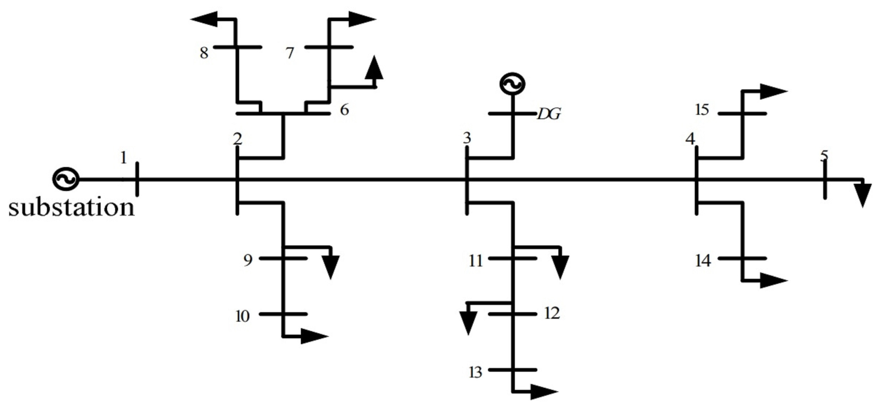
In this study on an IEEE 15-bus power grid, we employed the SINDy algorithm to analyze voltage waveforms and identify system dynamics under various complex operational scenarios. The choice of the experimental configuration was deliberate, aligning it with similar studies conducted by other researchers. The system architecture consists of 15 buses interconnected through branches representing power transmission lines, each with unique parameters and attributes governing power flow dynamics, as shown in Figure 2. Our discussion also encompasses the test scenarios, including abrupt changes and gradual load variations in the context of conventional SGs and IBRs at 50% and 100% integration. Our analysis serves as the foundation for introducing the Volterra-based nonlinearity index as a novel tool for assessing the order of nonlinearity in dynamic systems, offering significant insights into system dynamics.

3.1. Investigation Setup

The system architecture consists of 15 buses, representing distinct nodes within the power system network, and these buses are interconnected through branches that represent the power transmission lines. Each bus in the IEEE 15-bus system has a unique set of parameters and attributes and is connected to neighboring busses via branches characterized by specific impedance, which govern the dynamics of power flow among the interconnected buses.

Table 1. The implemented IEEE 15-bus-network configuration.

Line Index	From Bus	To Bus	r + xi (Ω)	Node Index	Pload + jQload (kW + kVAR)
1	1	2	1.53 + 1.778i	2	100 + j60
2	2	3	1.037 + 1.071i	3	90 + j40
3	3	4	1.224 + 1.428i	4	120 + j80
4	4	5	1.262 + 1.499i	5	60 + j30
5	5	9	1.176 + 1.335i	6	60 + j20
6	6	10	1.1 + 0.6188i	7	200 + j100
7	7	6	1.174 + 0.2351i	8	200 + j100
8	8	7	1.174 + 0.74i	9	60 + j20
9	9	8	1.174+ 0.74i	10	60 + j20
10	10	11	1.15+ 0.065i	11	45 + j30
11	11	12	1.274 + 1.522i	12	60 + j35
12	12	13	1.274 + 1.522i	13	60 + j35
13	13	14	1.075 + 1.522i	14	120 + j80
14	14	15	1.075+ 1.522i	15	60 + j10

provides a comprehensive overview of the network configuration and branch parameters of the IEEE 15-bus system.

This investigation explores a comprehensive set of power system conditions, encompassing both abrupt changes (faults) and gradual changes (load variations), in the context of conventional SGs and IBRs. The study encompasses three distinct scenarios, representing both single- and multi-dynamic systems. The first scenario examines a system solely supplied by a synchronous generator at Bus 1, with all other generators disconnected from the network. The second scenario incorporates the integration of an IBR at Bus 3, sharing the load demand equally with the synchronous generator at Bus 1. In the third scenario, the network is subjected to a 100% penetration of IBRs, where the demand is supplied by two IBRs located at Bus 1 and Bus 3. Each scenario spans 10 s, with the synchronous generators and IBRs initiated at $t=0\mathrm{s}$. At $t=3.3\mathrm{s}$, a three-phase-to-ground fault occurs at Bus 10, cleared after four cycles of the fundamental frequency (60 Hz). Furthermore, at $t=7\mathrm{s}$, a significant load is connected to Bus 14, only to be disconnected at $t=8\mathrm{s}$.

The SINDy algorithm, described in Algorithm 1, analyzed the acquired voltage waveforms, demonstrating promising system identification and modeling capabilities. Employing a refined computational approach, we consider essential parameters and algorithms to facilitate a comprehensive analysis. Careful consideration is given to the sampling rate (20,000 samples per second) and fundamental frequency (60 Hz) to ensure a high-fidelity representation of electrical phenomena. The simulation duration (10 s) and total sample count (200,000) are determined to capture temporal dynamics faithfully. By leveraging the Hilbert transform, converting voltage waveforms into complex numbers, and subsequent computation of instantaneous phase angles, we gain profound insight into the intricate behavior of the system.

Algorithm 1: The SINDy algorithm

Input:    Time history of the system’s state, denoted as v(t), where v(t)∈Rn.    Regularization parameter λ.    Library of candidate functions, Θ(V), where V is the data matrix that contains the observed data points of the system variables.    Step 1: Data Collection    Initialize empty matrices V and $\dot{V}$, where $\dot{V}$ represents the time derivatives of V.    For each time instance t in the set of time instances:    Collect data at time t and store it in v(t).    Compute the derivative of v(t) at time t, denoted as $\dot{v}$(t).    Append v(t) to the V matrix.    Append $\dot{v}$(t) to the $\dot{V}$ matrix.    Step 2: Construct Library of Candidate Functions    Initialize an empty list for the library of candidate functions.    For each candidate function in the set of candidate functions:    Compute the values of the candidate function using data matrix V.    Append the function values to the library.    Step 3: Sparse Regression    Initialize an empty list Ξ to store the sparse coefficient matrices for each variable.    For each system variable k:    Perform sparse regression using data matrices V, $\dot{V}$, the library Θ(V), and regularization parameter λ to obtain Ξk.    Sparse Regression Formulation:    The sparse regression problem for variable k can be expressed as follows:             $minimize{\left||\dot{V}-\Theta \left(V\right)\Xi |\right|}_2+\lambda {\left|\left|\Xi \right|\right|}_1$ where Ξk represents the sparse coefficient matrix for system variable k.    ${\left|\left|.\right|\right|}_2$ denotes the L2 norm.    ${\left|\left|.\right|\right|}_1$ represents the L1 norm.    λ is a regularization parameter that controls the trade-off between data fidelity and sparsity.    Step 4: Model Construction    Initialize an empty list for the models representing the system dynamics.    For each system variable k:    Construct the model for variable k using the library of candidate functions Θ(v) and the corresponding sparse coefficient Ξk.    Model Construction:    The model for system variable k can be expressed as follows:                 $v_k=\Theta \left(v\right){\xi }_k$ where Θ(v) is a vector of symbolic functions of the elements of v.    ${\xi }_k$ is the sparse vector of coefficients that determines the active terms in the system variable $v_k=f\left(v\right)$.    Output:    The list of models represents the system dynamics for each system variable, providing concise and accurate descriptions of the underlying nonlinear dynamics.

Furthermore, the simulation methodology incorporates the SINDy algorithm, wherein a polynomial library is constructed with up to a third-order polynomial and a regularization parameter (0.8). The ensuing coefficients derived from this process are then employed to solve the system’s ordinary differential equation, thus elucidating the underlying dynamics. Rigorous evaluation is conducted to assess the accuracy of the predicted slow dynamics and quantify the disparity between the identified fast dynamics and actual data.

Applying polynomial function libraries up to the third order in the context of inverter-based resources signifies a notable departure from traditional modeling approaches. In power grid modeling, mainly when dealing with inverter-based resources, these higher-order polynomial functions allow for a more intricate representation of the dynamic behavior within the system. Unlike first-order models that may oversimplify the interactions between various components, including polynomial functions up to the third order enables the capturing of nonlinearities and interactions characteristic of inverter-based resources. These functions provide a flexible framework to model the complex interplay between inverter controllers, grid conditions, and the response of renewable energy sources to changing environmental factors.

The application of these polynomial function libraries has theoretical and practical implications. Theoretically, it acknowledges the importance of capturing higher-order dynamics and interactions. It aligns with the principles of complex systems theory, emphasizing the significance of nonlinear dynamics and the emergence of complex behaviors in systems like power grids with significant inverter-based resource penetration. From a practical standpoint, this approach facilitates more accurate modeling, enabling grid operators and planners to understand better and predict the behavior of inverter-based resources. The practical advantages are particularly evident when renewable energy integration is critical. Through accommodating higher-order dynamics, these models enhance the ability to simulate, analyze, and optimize the grid’s performance, ultimately contributing to a more resilient and efficient power system.

Our investigation introduces a three-section data analysis structure, offering an enhanced approach to analyzing system dynamics. The initial two sections focus on identifying linear and nonlinear dynamics within the system, categorizing elements that are linearizable and those that are inherently nonlinear. The addition of the third section allows for managing negligible data components, ensuring improved modeling accuracy. This approach provides a more profound understanding of intricate nonlinear behaviors across various domains.

3.2. SG-Driven Power Grid Dynamic Identification

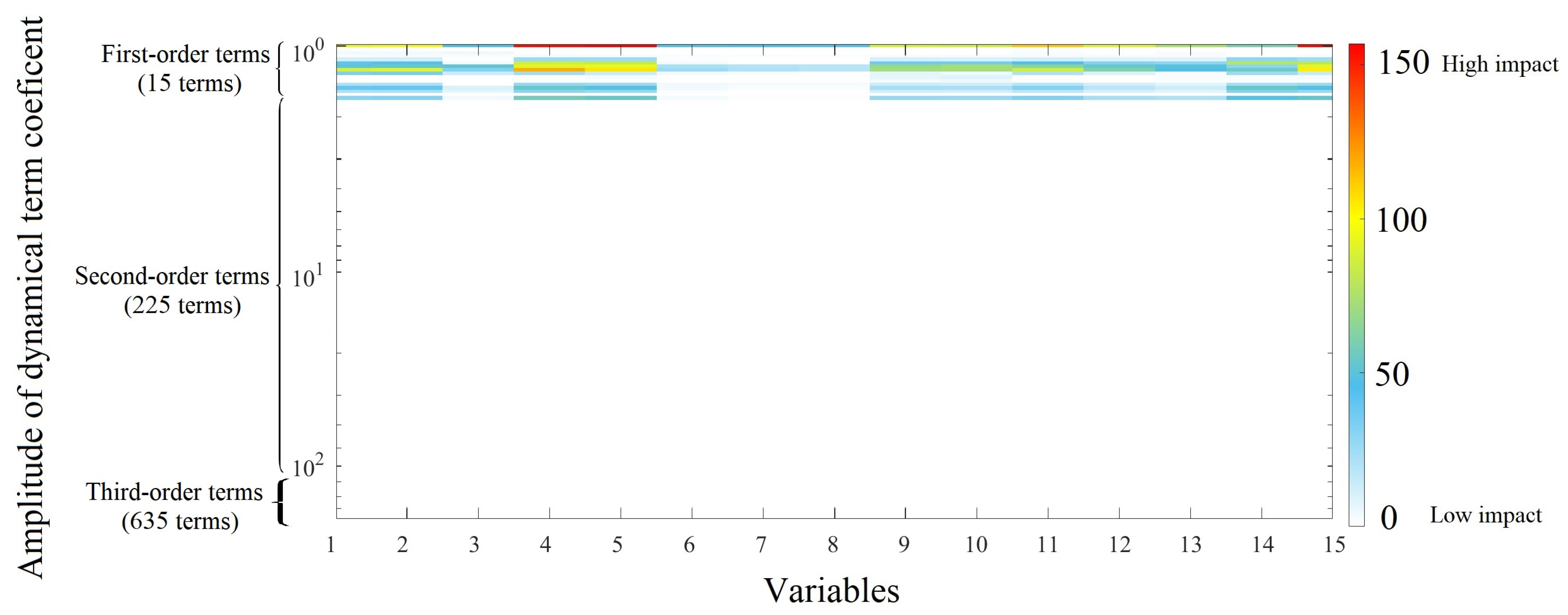
The study’s findings demonstrate that SINDy, with its utilization of voltage waveforms, successfully captures essential patterns and relationships within the electrical behavior of the power grid. The results highlight the potential of SINDy as a powerful tool for system identification and modeling in power systems. The results related to the SG model exhibit consistencies to foundation theories and findings from the other research. Our analysis highlights the dominance of first-order terms in the extensive 15-dimensional system. Second-order terms play minor roles, and third-order terms are close to zero, affirming the precision of our SINDy-based model with an impressively low error rate in capturing both short-term and long-term dynamics.

Figure 3 demonstrates that first-order terms dominate within the entire 15-dimensional system. In this case, the SG resources are modeled using the basic model. Second-order terms’ and third-order terms’ coefficients are negligible, approximated to zero using the MATLAB calculation.

The approximation of the system dynamics highlights the precision of the model estimated. The error between the actual data and the identified model’s approximation is impressively less than 0.001 percent, affirming the model’s accuracy in capturing both short-term and long-term dynamics.

To reduce the potential bias introduced by our choice of SG model, we replicated the investigation using a seventh-order SG model. This strategic adaptation allowed us to explore the impact of higher-order terms, primarily second-order terms, on the overall dynamics of the system. The result, presented in Figure 4, shows that the dynamics are still dominated by first-order terms where second-order-term coefficients are minimal, comprising less than 1 percent of the smallest first-order terms, and third-order term coefficients are even more negligible, approximated to zero using MATLAB (R2021a).

It is noteworthy that the appearance of second-order terms did not yield any significant effects, which aligns with the expectations set by current theoretical frameworks. The conventional understanding of power systems suggests that higher-order terms, particularly those that are second order, tend to play a relatively minor role in system behavior, especially when compared to the prominence of first-order terms. This observation underscores the consistency of our findings with established theoretical principles, reaffirming the accuracy and reliability of our analysis.

From a system analysis perspective, the prominence of the first-order terms in the analysis indicates that the nondiagonal eigenvalues of the system are nonvital. Consequently, the system does not exhibit considerable system-level interactions and can be characterized as linear or quasi-linear. This linearity suggests that the system is linearly stabilizable from a monitoring and control standpoint. Furthermore, the assertion extends to the system’s linearity, implying that the system response is proportional to the applied inputs and obeys the principle of superposition. This linearity facilitates the analysis and control design, allowing for the use of linear control strategies without resorting to nonlinear or complex control approaches. Furthermore, these dominant terms dictate the rate of decay or growth of disturbances, directly impacting system stability and reflecting the system’s ability to withstand disturbances and recover stability.

From a Fourier series analysis perspective, the dominance of first-order terms in the system underscores the critical influence of fundamental-frequency components on system dynamics. This prominence suggests that the system’s behavior is primarily characterized by these fundamental oscillations, with higher-order contributions playing a secondary role, resulting in the system exhibiting minimal harmonic distortion.

3.3. Dynamic Identification in IBR-Integrated Power Grid

Through conducting the investigations on the power system integrated with IBRs, this section navigates through these distinct nonlinear behaviors, grounded in the principles of complex systems theory and nonlinear dynamics, to offer valuable insights into the dynamic response of power grids with substantial IBR integration. The results embark on an exploration of the dynamic behavior of IBRs within a power grid, shedding light on the distinctive difference in the nature of nonlinear dynamics caused by IBRs and SGs. The nonlinearity in SGs is characterized as “module-level dynamic nonlinearity,” which is rooted in well-documented electromagnetic principles and iron core saturation effects, primarily influenced by the individual components of SGs. In contrast, the nonlinearity encountered in IBRs reveals a multifaceted character, encompassing both module and system-level nonlinearity. The latter, system-level nonlinearity, is a product of intricate interactions between diverse components, control algorithms, and the inherent variability of input sources, indicative of complex system dynamics.

The investigation will analyze two scenarios. The first scenario will conduct the test over the same IEEE 15-bus system that is supplied using both the basic SG model and IBR where each supplies 50% of the load demand. The second scenario will investigate the same power system under full penetration of IBRs, i.e., 100% of the load demands are supplied with IBRs.

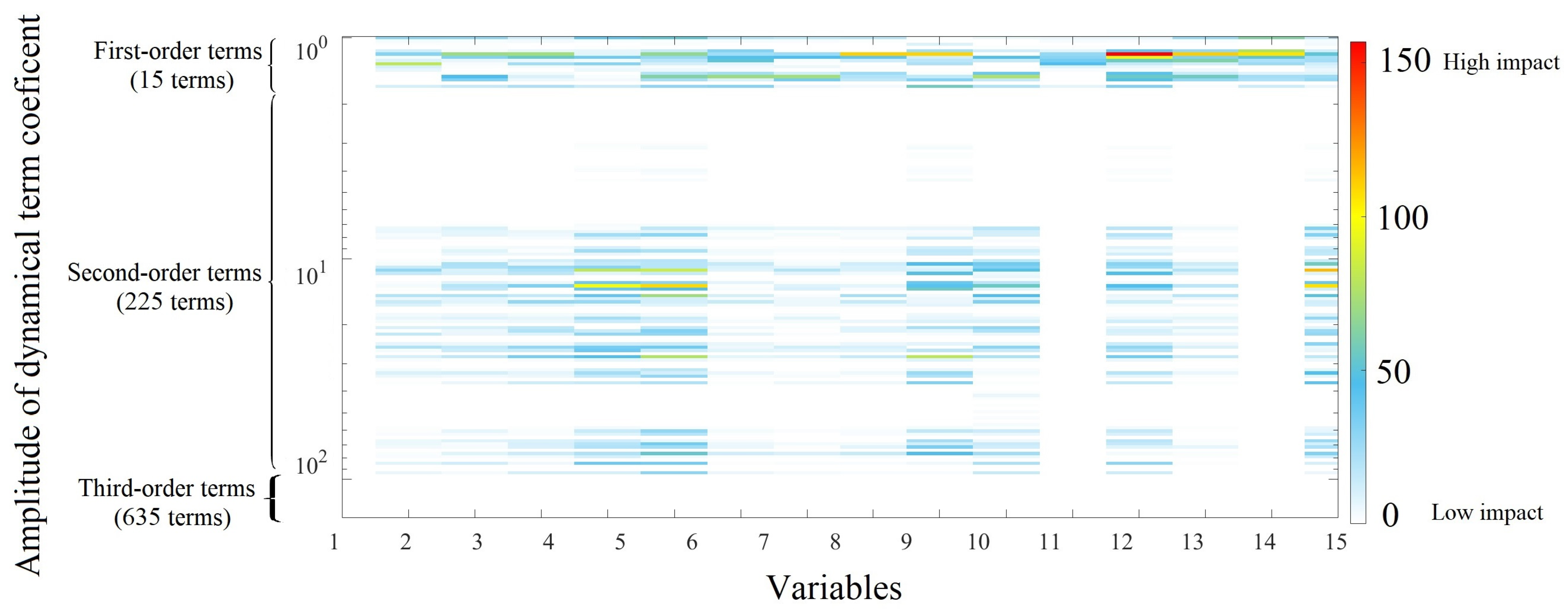
Through the first scenario with 50% integration of inverter-based resources into the power grid, equalizing their role with SGs in supplying load demands, the SINDy algorithm was used to identify the underlying dynamic with the measured data. As Figure 5 illustrates, it was found that the second-order terms become more effective in the dynamic model. The higher impact of the second-order terms will show that the data-based model, i.e., the underlying model within measurements, has a more nonlinearizable nature that shows itself in higher coefficient values for second-order terms. However, the third-order terms, representing the negligible data (noise) are still in the same condition.

The results unveil a noteworthy transformation in the power grid dynamics during our exploration of IBR integration. What becomes evident is not only the heightened influence of second-order terms (characterizing nonlinear dynamics) on the system’s overall behavior within all the individual buses but also the activation of more terms in the second-order region, thus highlighting the unmistakable imprint of system-level nonlinearity on outcomes. This intriguing shift underscores the intricate interplay of components in the network and the inherent variability in each source, collectively contributing to the observed system-level nonlinearity. In comparison to previous scenarios, this outcome signifies a fundamental difference, illuminating how power grids evolve when IBRs are introduced, revealing a dynamic that transcends more module dynamics and delves into the realm of complex, system-wide nonlinear interactions.

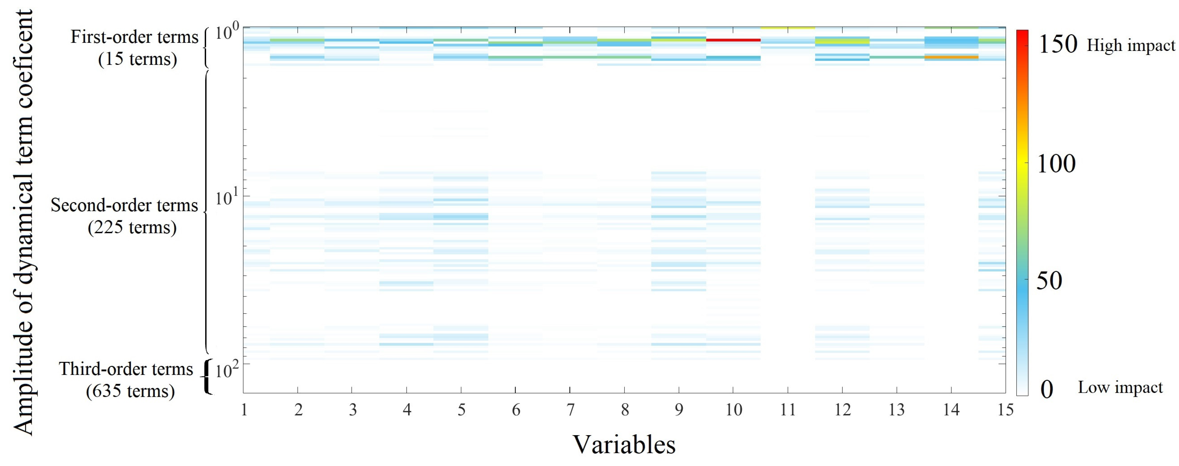
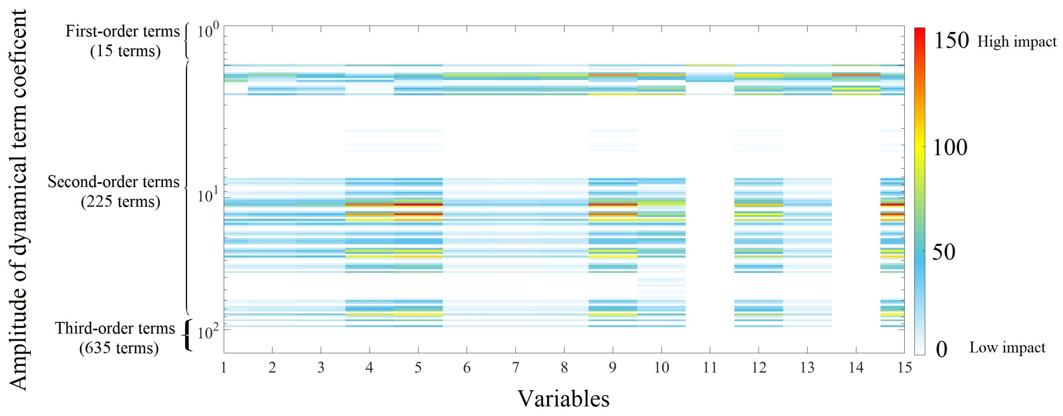
In the next scenario, where load demands were exclusively supplied by IBRs, our model identification analysis, as depicted in Figure 6, remarkably underscored the dominance of second-order terms. This shift in the composition of dominant terms is a pivotal result that merits in-depth discussion. The prominence of second-order terms in this context carries profound implications for understanding power grid dynamics.

This outcome indicates the profound impact of IBR-related nonlinearity on the power grid, highlighting the necessity for more nuanced modeling to represent these complex interactions accurately. The dominance of second-order terms indicates that these nonlinear behaviors have a substantial impact on the system’s dynamics. In the context of IBRs, it becomes evident that second-order terms play a key role in capturing and representing the system’s response to these nonlinear effects. This underscores the need to consider and model the nonlinearity introduced by IBRs explicitly, as first-order models may need to be revised to represent these intricate interactions.

Moreover, from a theoretical perspective, this result aligns with the established principles of nonlinear system dynamics. In complex systems, it is expected that we observe higher-order nonlinearities, especially when the interactions among system components are intricate. These second-order terms can arise due to a variety of reasons, including feedback mechanisms, nonlinear-component characteristics, and complex system interactions.

Furthermore, a noteworthy observation emerged when comparing the level of participation of second-order terms in the 100% penetration of IBRs to the 50% and 0-penetration scenarios. This comparison, presented in Figure 7, accentuated a significant shift, indicative of the substantial impact of variable interactions in contrast to the direct effects of individual variables on the system’s dynamics.

As observed, the analysis of the seventh-order SG model underscores the prevalence of first-order terms, indicative of linearizable dynamics within the measured data. The limited influence of high-order terms and noise in this model allows for their neglect without substantially affecting the model’s accuracy. Furthermore, the nonlinearity in this context is primarily associated with the individual buses connected to SG sources, suggesting a module-level nonlinearity.

In scenarios featuring 50% and 100% integration of IBRs, a notable increase in nonlinearity is evident, which is manifested as higher coefficients for second-order terms. It is worth noting that the integration of IBRs activates a greater number of terms, and these activated terms are not directly linked to the buses connected to IBR sources, indicating the emergence of system-level nonlinearity resulting from network interactions. The graphical representation vividly portrays the escalating nonlinearity and the increasing influence of second-order terms as IBR penetration rises from 50% to 100%, ultimately leading to the dominance of nonlinear dynamics in the overall system behavior.

From a system analysis perspective, when high-order terms dominate the dynamics, it implies a departure from the conventional understanding associated with the prominence of first-order terms. In this scenario, the system’s nondiagonal eigenvalues become vital indicators of system behavior. The dominance of high-order terms suggests increased complexity and nonlinearity in system dynamics, potentially leading to stronger system-level interactions and a departure from linear or quasi-linear behavior. Consequently, the eigenvalues associated with these high-order dynamics play a crucial role in determining system stability, with their characteristics influencing stability margins and critical clearing times. Understanding and analyzing these eigenvalues become imperative for assessing system stability and designing effective control strategies.

From a Fourier series analysis perspective, the dominance of high-order terms unveils a more intricate system response characterized by a broader range of frequency components, leading to a richer harmonic content in the system’s response. This phenomenon enriches the harmonic content within the system’s response, aligning with authors’ previous findings [30]. Such heightened complexity underscores the necessity for thorough frequency–domain analysis to comprehend the breadth of system behavior fully.

3.4. Volterra-Based Nonlinearity Index

In dynamic systems, the interplay between linear and nonlinear behaviors is a common phenomenon, and quantifying this nonlinearity holds paramount importance for comprehending system performance, facilitating effective control, and optimizing signal processing. In this study, the Volterra-based nonlinearity index (VNI) is introduced as a novel analytical instrument with the capacity to evaluate nonlinearity in dynamic systems quantitatively. This section not only introduces the fundamental concept of VNI but also explores its mathematical underpinnings. The VNI’s significance transcends this, as it enables the quantification of the nonlinear-to-linear relationship within dynamic systems, offering profound insights into the intricate dynamics at play. Moreover, the VNI’s versatility allows for the recognition of different types of nonlinearities and the quantification of the relative influences of system-level and module-level nonlinearity, further enhancing its utility in system analysis and modeling. Using the case studies conducted in this research, we showcase practical experiments employing VNI, revealing new discoveries regarding nonlinearity in the seventh-order SG model compared to IBRs. These discoveries highlight different patterns of nonlinearity and emphasize the importance of structural analysis in identifying their sources.

Since dynamic systems often exhibit a combination of linear and nonlinear behaviors, characterizing the extent of nonlinearity is pivotal in understanding system performance, control, and signal processing. To elucidate the impact of high-order terms and to highlight the effectiveness of the SINDy in capturing system dynamics, we introduce a novel index that assesses the influence of high-order dynamics. The VNI is an analytical tool designed to assess the level of nonlinearity in dynamic systems quantitatively. The VNI draws its foundation from the Volterra series [16], a powerful mathematical construction that dissects system responses into linear and higher-order nonlinear components, providing a systematic approach to nonlinear modeling and analysis [31].

VNI is expressed as the ratio of the energy (or magnitude) associated with the nonlinear components to the energy of the linear response within the Volterra series expansion. This formulation encapsulates the inherent nonlinearity of the system and the interplay between linear and nonlinear phenomena. Mathematically, VNI is defined as follows:

$$VNI=\frac{\sum _{k=1}^N\iint {\left|H_k\left({\tau }_1,{\tau }_2\right)\right|}^{2}d{\tau }_{1}d{\tau }_2}{{\left|H_0\right|}^2}$$

(12)

Here, N represents the selected order of the Volterra series, accommodating the analysis of a range of higher-order nonlinear terms. $H_k\left({\tau }_1,{\tau }_2\right)$ signifies the Volterra series coefficients on the kth order nonlinear terms, and ${\left|H_0\right|}^2$ represents the squared magnitude of the linear response.

A higher VNI value implies a greater prevalence of nonlinearity in the system. Consequently, VNI serves as a comprehensive gauge of the nonlinear-to-linear relationship within a dynamic system, contributing to a more profound understanding of the system’s dynamics and its suitability for specific applications.

It has to be noted that the application of machine learning approaches to the VNI introduces an exciting dimension in the realm of system analysis and modeling. VNI, when coupled with machine learning techniques, can unlock the potential to discern and differentiate various types of nonlinearities inherent within complex dynamic systems. Machine learning algorithms recognize patterns, relationships, and hidden structures within data, and, when applied to VNI data, they can extract nuanced distinctions in the system’s behavior. These distinctions manifest as different types of nonlinearities that are challenging to identify using conventional methods. This capability has significant implications for characterizing the complex behavior of systems with mixed linear and nonlinear components relying on measurement-based and real-time methods, as it can provide insights into how different nonlinear phenomena manifest and interact in the overall system response.

The VNI framework could be utilized in diverse applications across science and engineering disciplines. In control systems, it aids in assessing the stability and robustness of nonlinear control strategies, informing the choice of appropriate controllers. In communication systems, it provides insights into signal quality, especially in scenarios where nonlinear effects can degrade signal integrity. In physical and biological systems, VNI enables researchers to quantify and understand the nonlinear interactions underlying complex behaviors.

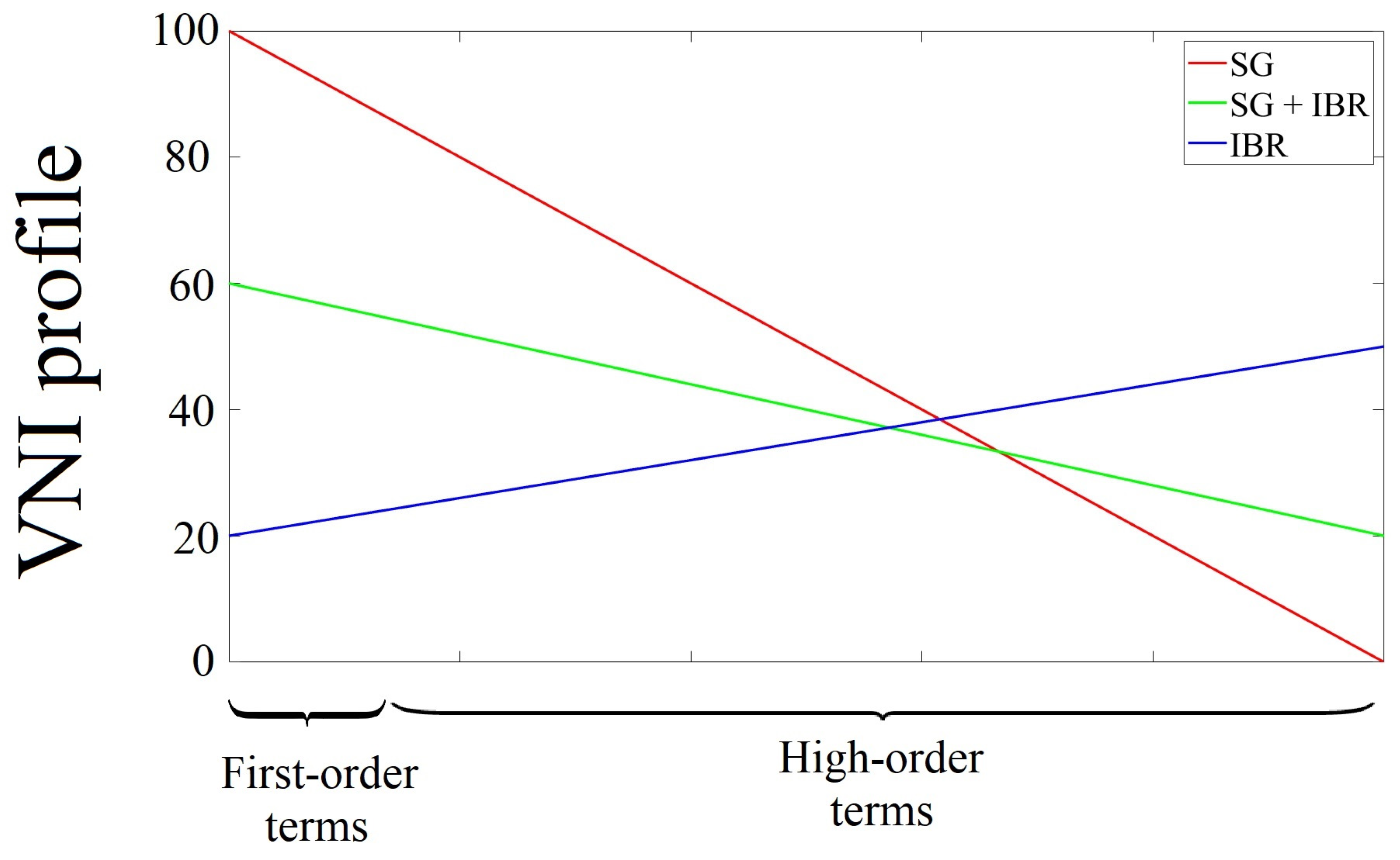
Applying the VNI and VNI profile to the case studies in our investigations, the VNI values for three scenarios in the system were supplied with seventh-order SGs, a combination of basic model SGs and IBRs, and the IBRs were calculated equal to 0.78, 0.54, 3.54, respectively.

To have a visual indicator of the extent of nonlinearity within the dynamic system the VNI profile, as a novel concept used to assess the linearity and nonlinearity within dynamic systems, particularly in system-level interactions is introduced. It is based on the proposed VNI, which quantitatively measures the level of nonlinearity within a dynamic system. The VNI profile associates a profile with the identified dynamics of the system, explicitly relating the slope of the profile, r, to the calculated VNI value through the following relation:

$$r=VNI-1$$

(13)

This relationship provides a means to classify the prevalence of either linearity or nonlinearity within the system. The calculation of the VNI profile for each case study serves to distinctly illustrate and visualize the distinctions in both the magnitude and character of nonlinearity between them. When the VNI profile exhibits a negative slope, it suggests that linearity dominates the system dynamics. In this scenario, the higher-order terms have less influence on the overall dynamics, indicating that the system’s behavior is primarily linear or that nonlinearity is confined to a module level. This means that linear relationships can predominantly explain the system’s response, and the impact of higher-order terms is limited.

Conversely, when the VNI profile shows a positive slope, it signifies the domination of nonlinearity within the system and suggests that the higher-order terms have a more significant impact on the overall dynamics. In such cases, nonlinearity is not confined to module-level interactions but extends to system-level interactions. Through analyzing this profile, researchers and engineers can understand whether linearity or nonlinearity predominates in a given system and whether the nonlinearity is confined to the module level or extends to system-level interactions. The estimated VNI profiles of the scenarios with seventh-order SGs, a combination of basic model SGs and IBRs, and the IBRs are presented in Figure 8.

4. Conclusions

This paper contributes to the field of power system analysis by employing the SINDy method, exploring a range of conditions, including abrupt faults and gradual load variations. This methodology ensures robustness, generalization potential, and the identification of key dynamical features utilizing voltage measurements, thereby advancing our theoretical understanding of power system analysis. Introducing the Volterra-based nonlinearity index in this paper, the study distinguishes first- and high-order active terms in the system’s governing equation. The VNI characterizes system-level nonlinearity through differentiating between first-order linearizable terms, second-order nonlinear dynamics, and third-order noise, providing a comprehensive grasp of power systems’ intricacies. The results showed a fundamental shift in system dynamics as power sources transition to IBRs, revealing system-level nonlinearity compared to module-level nonlinearity in conventional generators. The proposed index quantifies nonlinear-to-linear relationships, enriching our understanding of power system behavior and offering a valuable tool for discerning different nonlinearities and visualizing their distinct patterns through the index’s profile. The introduction of higher-order polynomial function libraries to model IBR integration marks a significant departure from traditional approaches, reflecting the evolving needs of power grid analysis as renewable energy takes center stage.

The relevance of the findings regarding the influence of dominant terms on system eigenvalues extends to established methodologies such as dynamic phasor modeling, state estimation, and optimal power flow. Dynamic phasor modeling, which approximates the dynamic behavior of power systems using phasor representations, relies on accurate characterization of system eigenvalues to capture transient stability and dynamic response. By understanding the impact of dominant terms on eigenvalues, dynamic phasor models can better simulate system behavior under varying operating conditions, enhancing stability assessment and control design. Similarly, in state estimation, accurate estimation of system states and parameters is crucial for real-time monitoring and control. Knowledge of dominant terms aids in refining state estimation algorithms, improving the accuracy of system state estimates, and enhancing situational awareness. Furthermore, in optimal power flow studies, where the objective is to optimize power system operation while satisfying operational constraints, considering system eigenvalues influenced by dominant terms enables a more precise assessment of system stability limits and helps identify optimal operating points that maximize efficiency and reliability.

The practical implications of these findings are substantial for power grid operators and planners. By utilizing the introduced VNI and the insights gained from the SINDy method, operators can better assess and manage the dynamic behavior of power systems. This knowledge enables more accurate predictions of system-level nonlinearity, helping to anticipate and address potential challenges associated with the transition from conventional generators to IBRs.

Additionally, the ability to quantify nonlinear-to-linear relationships through the proposed index offers a practical tool for optimizing grid performance. Grid operators can use this information to fine-tune control strategies, improve grid stability, and enhance operational efficiency. The departure from traditional modeling approaches, especially with the introduction of higher-order polynomial function libraries for IBR integration, reflects a forward-looking perspective that aligns with the evolving landscape of renewable energy. This shift provides practical solutions for building resilient and efficient grids capable of accommodating the increasing penetration of renewable energy sources.

The complexities of modern power systems demand ongoing research and development to refine our tools and approaches. Future investigations could further enhance our ability to detect and identify sources of oscillations in real-time, a crucial step towards ensuring the stability and reliability of our power grids.