A Fault Location Algorithm for Multi-Section Combined Transmission Lines Considering Unsynchronized Sampling

Abstract

This paper introduces a fault location technique for multi-section combined transmission lines, utilizing unsynchronized fault record data. The approach determines the intersection points of the voltage magnitudes computed using the fault current and voltage records of each terminal and the constant line parameters of each section. Finally, the real fault location is identified based on the calculated inverse angle of equivalent impedance. To evaluate the performance of the proposed algorithm, a three-section combined transmission line is constructed using the PSCAD/EMTDC software version 5.0.0, and various fault scenarios are simulated and tested employing the proposed algorithm. The results indicate that the proposed algorithm is applicable to various types of faults in a multi-section combined transmission line; the estimations are accurate.

1. Introduction

An overhead transmission line is typically used to send electricity from power stations to substations near consumers. However, the use of underground cables has become imperative and is mandated by the environmental constraints imposed on construction sites in urban areas. This has triggered the development of hybrid transmission systems that combine both overhead and underground lines. Precise fault location minimizes the time and expense associated with deploying crews to search for faults. The enhancement of customer service and ensuring that consumers experience minimal interruptions improve the power system performance and pinpoint weak or vulnerable points [1,2]. Moreover, accurate fault location enhances the availability and reliability of power systems [3]. As the constant line parameters of overhead and underground transmission lines differ significantly, the accuracies of homogenous transmission line fault location methods [4,5,6,7] must be re-examined. A fault location approach that considers the non-homogeneity of combined transmission lines is required. Furthermore, it is crucial to take into account the effects of the unsynchronized sampling resulting from varying record starting times in different fault recorders when implementing a multi-terminal fault location algorithm.

1.1. Literature Review

This section highlights promising fault location approaches for combined transmission lines. The existing algorithms are based on neural networks, traveling wave evaluations, and impedance characteristics.

The use of artificial neural networks for fault detection, classification, and localization is discussed in [8,9]. The model of [8] utilizes the phasors of the three-phase voltage and current as inputs. In contrast, the approach of [9] requires only instantaneous current data. Although both methods are very accurate, they are applicable to only homogeneous transmission lines. The reports in [10,11,12] used artificial neural networks to estimate the fault distances along combined transmission lines. These methods require two sequential steps. Initially, the faulted section is identified, followed by the estimation of the fault distance. The method of [10] uses a support vector machine to identify the faulted section. An adaptive network-based fuzzy inference system with four inputs is employed in [11] for fault location training. Report [12] presents a novel scheme that detects, classifies, and locates faults in two- and multi-terminal transmission lines. This scheme employs the fast-discrete orthogonal S-transform (FDOST) in conjunction with a support vector machine. The three-phase currents are measured at the line ends to derive the entropies of the FDOST coefficients; the coefficients are then input to a support vector regression module to detect the fault location. However, in all of the methods of [8,9,10,11,12], retraining is necessary when the system configuration changes substantially.

Traveling wave-based algorithms are more precise than impedance-based algorithms and are not affected by the source impedance, fault resistance, or power flow [13]. In many traveling wave methods, the high-frequency transients generated by faults are employed to accurately determine the fault locations. Despite these advantages, the algorithms are susceptible to noise, faults on other lines, the fault inception angle, reflected waves from other terminals, and equipment that lies beyond the relay and fault points [14]. Additionally, these methods do not deal well with faults close to the terminals [15]. A method that combined traveling wave analysis with samples of the high-frequency voltage transients generated by faults in two terminals is highlighted in [16]. This approach relies on wavelet analysis; the wave speed is irrelevant. The methods of [17,18,19] do not employ fault-generated high-frequency transients, rather using high-frequency fault-clearing transients to cope with problems. The method of [19] uses a single-ended approach to derive a fault location algorithm for combined transmission lines. Neither the overhead line data nor the cable parameters are required.

There are two types of fault location methods based on impedance: single-ended and multiple-ended. In the methods of [20,21], single-ended measurements are employed. The superposition principle is used to estimate the fault locations on a transmission line. In [22], ground distance protection was adapted to suit a cascaded transmission line consisting of overhead and submarine cables. Although communication is thus not required, algorithms that employ single-ended data may be inaccurate if the source impedances, fault inception angles and/or impedances, and loading conditions vary. The challenges associated with this single-ended method were addressed by employing two-terminal synchronized data provided by a Global Positioning System-based synchronous measuring unit [23,24,25]. The approaches of [26,27,28,29] ensure accurate fault location in the absence of synchronization. Although these methods are very accurate (regardless of the fault resistance), they are suitable for only homogeneous transmission lines. The method of [30] employs synchronized measurements for fault detection and location in a two-section line with both an overhead line and an underground power cable; it is essential to identify the fault type prior to pinpointing the fault location. Importantly, the method is specifically designed for use with two-section compound transmission lines; it does not handle more general multi-section compound lines. In [31], the applications of the algorithm are expanded to cover more than two sections. The algorithm initially assumes a fault in each section, and the fault locations are both determined. Ultimately, only the section that delivers a correct answer within the range of interest is identified as an actual fault. In [32], a novel method for fault identification is introduced. The approach is based on the rate of the change in voltage along a non-homogeneous line in a positive-sequence circuit. The faulted side is identified using a novel specific formula. Subsequently, the fault distance is calculated based on analysis of the identified fault section. Importantly, the methods of [31,32] both require synchronized measurement data. In [33], a fault location scheme devoid of parameters was introduced to estimate the location of faults on a hybrid transmission line, employing unsynchronized data; however, it considers only a two-section transmission line.

1.2. Our Motivation and Contributions

The inhomogeneity of combined underground/overhead transmission lines renders fault location techniques based on distributed parameters difficult regardless of whether single- or dual-ended applications are employed. Apart from the effects of fault resistance, single-ended methods do not handle variations in the positive-sequence impedance per unit length well; this parameter is critical when seeking to determine the fault location. Thus, the precision of traditional algorithms fluctuates considerably as the fault distance varies. Although several approaches seek to locate faults on multi-section combined transmission lines, most require high sampling rates or synchronized sampling, which are expensive and difficult to achieve in real-world applications. The main objective of this paper is the development of a fault location algorithm that addresses the abovementioned challenges. The process is divided into two stages. First, the intersection points between the voltage magnitudes, computed using the fault currents and voltages recorded at each terminal, are determined employing an incremental increase approach. Next, a real fault identification algorithm is applied to the identified intersection point. If this is not a real fault location, that point is rejected, and the process continues until a real fault is located. The proposed algorithm offers several advantages:

• Fault locations on combined transmission lines can be accurately estimated even when the fault record sampling data are not synchronized,
• The performance of the proposed algorithm remains accurate under various types of faults, fault resistances, fault inception angles, and sources of impedance variation,
• Faults are accurately located even if they lie very close to interconnection points,
• The proposed algorithm can be modified to accommodate different numbers of sections according to real-world applications.

The remainder of this study is organized as follows. In Section 2, the details of the proposed fault location algorithm are described. In Section 3, the estimated fault location for different fault conditions depending on different fault resistance, fault locations, fault types, and phase errors are presented. Section 4 concludes the study and mentions planned future work.

2. The Fault Location Algorithm

This section presents the principles and approaches utilized for fault location estimation on a combined transmission line with unsynchronized sampling consideration. To facilitate understanding in the subsequent section, a list of relevant acronyms and their definitions is provided in

Table 1. The relevant acronyms and their definitions.

Acronym	Units	Definition
cnt_max		Maximum iteration number
d	pu	Different voltage magnitude
F	km	Fault location
FDOST		Fast-discrete orthogonal S-transform
FPrev	km	Estimated fault location of the previous sample
F’	km	Voltage magnitude intersection point but not a real fault
LP1, LP2, L	km	Distance from the S terminal to points M and N and total length
M, N		Interconnection points on the combined transmission line
P1, P2, P3		Sections on the combined transmission line
VF, IF		Fault voltage and current
VMR1, IMR1, VNR1, INR1	pu	Positive-sequence voltage and current at the points of interconnection M and N computed based on R terminal data
VMS1, IMS1, VNS1, INS1	pu	Positive-sequence voltage and current at points M and N computed based on S terminal data
VS, IS, VR, IR	pu	Three-phase voltage and current at the S and R terminals
VS1, IS1, VR1, IR1	pu	Positive-sequence voltage and current at the S and R terminals
VXR, IXR	pu	Three-phase voltage and current at point X computed based on R terminal data
VXR1, IXR1	pu	Positive-sequence voltage and current at a specific point along the transmission line computed based on R terminal data
VXS, IXS	pu	Three-phase voltage and current at point X computed based on the S terminal data
VXS1, IXS1	pu	Positive-sequence voltage and current at a specific point along the transmission line computed based on S terminal data
X		Voltage magnitude computation point
x	pu	Distance from S terminal to point X
Y1, Y1_P1, Y1_P2, Y1_P3	pu	Positive-sequence admittance of the homogenous transmission line and sections P1, P2, and P3 of the combined transmission line
ZC1, Z C1_P1, Z C1_P2, Z C1_P3		Positive-sequence characteristic impedance of the homogenous transmission line and sections P1, P2, and P3 of the combined transmission line
Zeq		Equivalent impedance
Z1, Z1_P1, Z1_P2, Z1_P3	pu	Positive-sequence impedance of the homogenous transmission line and sections P1, P2, and P3 of the combined transmission line
${\mathsf{\gamma }}_1$, ${\mathsf{\gamma }}_{1\_\mathrm{P}1}$, ${\mathsf{\gamma }}_{1\_\mathrm{P}2}$, ${\mathsf{\gamma }}_{1\_\mathrm{P}3}$		Positive-sequence propagation constant of the homogenous transmission line and sections P1, P2, and P3 of the combined transmission line
α		Increasing rate
δ		Perturbation value
ε		Margin for phasor estimation error
${\mathsf{\phi }}_{\mathrm{IEZ}}$		Inverse angle of the equivalent impedance

.

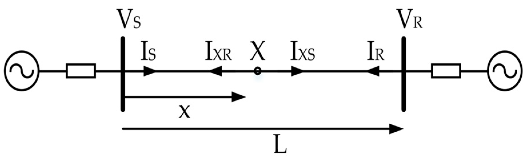
2.1. Voltages and Currents along the Homogenous Transmission Line

The single-line diagram in Figure 1 shows a homogenous transmission line of total distance L. V_S, I_S, V_R, and I_R are the three-phase voltage and current measurements at terminals S and R, respectively. V_S1, I_S1, V_R1, and I_R1 are the positive-sequence voltage and current components derived from V_S, I_S, V_R, and I_R by using symmetrical component transformation. The positive-sequence voltage and current along the transmission line at distance x from terminal S then can be computed based on the S and R terminal measurement data, as written in Equations (1) and (2) [34].

$$\left[\begin{array}{c}{\mathrm{V}}_{\mathrm{XS}1}\\ {\mathrm{I}}_{\mathrm{XS}1}\end{array}\right]=½\left[\begin{array}{cc}{\mathrm{e}}^{{\mathsf{\gamma }}_1\mathrm{x}}+{\mathrm{e}}^{-{\mathsf{\gamma }}_1\mathrm{x}}& -{\mathrm{Z}}_{\mathrm{C}1}({\mathrm{e}}^{{\mathsf{\gamma }}_1\mathrm{x}}-{\mathrm{e}}^{-{\mathsf{\gamma }}_1\mathrm{x}})\\ -1/{\mathrm{Z}}_{\mathrm{C}1}({\mathrm{e}}^{{\mathsf{\gamma }}_1\mathrm{x}}-{\mathrm{e}}^{-{\mathsf{\gamma }}_1\mathrm{x}})& {\mathrm{e}}^{{\mathsf{\gamma }}_1\mathrm{x}}+{\mathrm{e}}^{-{\mathsf{\gamma }}_1\mathrm{x}}\end{array}\right]\left[\begin{array}{c}{\mathrm{V}}_{\mathrm{S}1}\\ {\mathrm{I}}_{\mathrm{S}1}\end{array}\right],$$

(1)

$$\left[\begin{array}{c}{\mathrm{V}}_{\mathrm{XR}1}\\ {\mathrm{I}}_{\mathrm{XR}1}\end{array}\right]=½\left[\begin{array}{cc}{\mathrm{e}}^{{\mathsf{\gamma }}_1(\mathrm{L}-\mathrm{x})}+{\mathrm{e}}^{-{\mathsf{\gamma }}_1(\mathrm{L}-\mathrm{x})}& -{\mathrm{Z}}_{\mathrm{C}1}({\mathrm{e}}^{{\mathsf{\gamma }}_1(\mathrm{L}-\mathrm{x})}-{\mathrm{e}}^{-{\mathsf{\gamma }}_1(\mathrm{L}-\mathrm{x})})\\ -1/{\mathrm{Z}}_{\mathrm{C}1}({\mathrm{e}}^{{\mathsf{\gamma }}_1(\mathrm{L}-\mathrm{x})}-{\mathrm{e}}^{-{\mathsf{\gamma }}_1(\mathrm{L}-\mathrm{x})})& {\mathrm{e}}^{{\mathsf{\gamma }}_1\mathrm{x}}+{\mathrm{e}}^{-{\mathsf{\gamma }}_1(\mathrm{L}-\mathrm{x})}\end{array}\right]\left[\begin{array}{c}{\mathrm{V}}_{\mathrm{R}1}\\ {\mathrm{I}}_{\mathrm{R}1}\end{array}\right],$$

(2)

Z_C1 = $\sqrt{{\mathrm{Z}}_1/{\mathrm{Y}}_1}$ represents the positive-sequence characteristic impedance and ${\mathsf{\gamma }}_1$ = $\sqrt{{\mathrm{Y}}_1 \times {\mathrm{Z}}_1}$ is the positive-sequence propagation constant. Z₁ and Y₁ are the positive-sequence series impedance and shunt admittance of the transmission line.

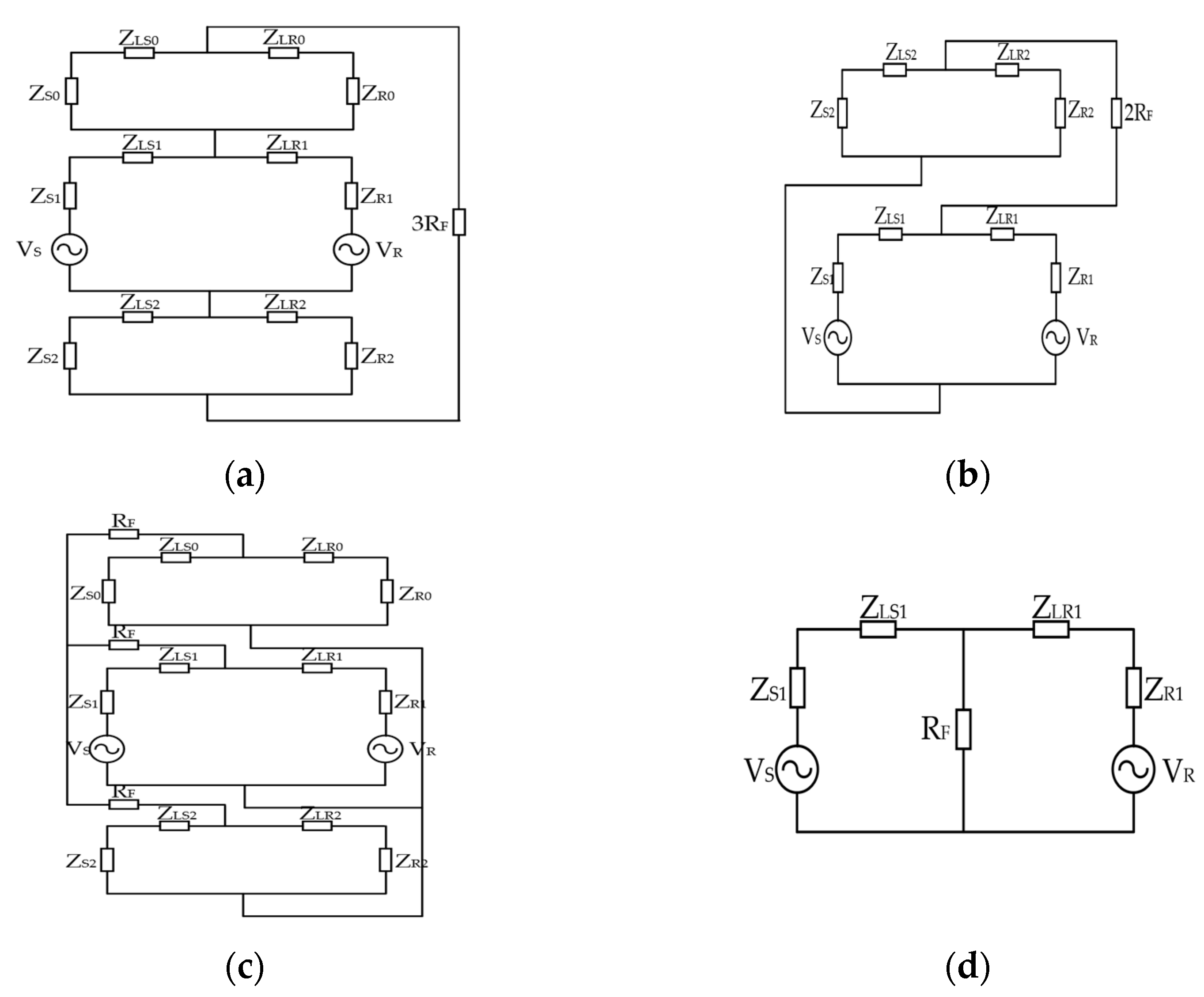
2.2. Voltages and Currents along the Three-Section Combined Transmission Line

In contrast to the homogeneous transmission line, where the voltage and current along the line can be calculated using the measurement data from each terminal, for an inhomogeneous line, these values can be computed solely based on the voltage and current at the nearest interconnection point. The voltage and current at the interconnection point are determined based on the voltage and current up to the terminal.

The single-line diagram in Figure 2 shows a three-section combined transmission line of total distance L. The transmission line is segmented into the three components P1, P2, and P3, where L_P1 and L_P2 are the lengths from terminal S to the interconnection points M and N. V_S, I_S, V_R, and I_R are the three-phase voltage and current measurements at terminals S and R, respectively. V_S1, I_S1, V_R1, and I_R1 are the positive-sequence voltage and current components derived from V_S, I_S, V_R, and I_R. The positive-sequence voltage and current along the transmission line at a specific point distance x from terminal S can then be computed based on the S and R terminal fault record data using Equations (3) and (4).

$$\left[\begin{array}{c}{\mathrm{V}}_{\mathrm{XS}1}\\ {\mathrm{I}}_{\mathrm{XS}1}\end{array}\right]=\left\{\begin{array}{c}½\left[\begin{array}{cc}{\mathrm{e}}^{{\mathsf{\gamma }}_{\mathrm{P}1}\mathrm{x}}+{\mathrm{e}}^{{-\mathsf{\gamma }}_{\mathrm{P}1}\mathrm{x}}& -{\mathrm{Z}}_{\mathrm{C}1\_\mathrm{P}1}({\mathrm{e}}^{{\mathsf{\gamma }}_{\mathrm{P}1}\mathrm{x}}-{\mathrm{e}}^{{-\mathsf{\gamma }}_{\mathrm{P}1}\mathrm{x}})\\ {-{1/\mathrm{Z}}_{\mathrm{C}1\_\mathrm{P}1}(\mathrm{e}}^{{\mathsf{\gamma }}_{\mathrm{P}1}\mathrm{x}}-{\mathrm{e}}^{{-\mathsf{\gamma }}_{\mathrm{P}1}\mathrm{x}})& {\mathrm{e}}^{{\mathsf{\gamma }}_{\mathrm{P}1}\mathrm{x}}+{\mathrm{e}}^{{-\mathsf{\gamma }}_{\mathrm{P}1}\mathrm{x}}\end{array}\right]\left[\begin{array}{c}{\mathrm{V}}_{\mathrm{S}1}\\ {\mathrm{I}}_{\mathrm{S}1}\end{array}\right] , \mathrm{if} (\mathrm{x} \le { \mathrm{L}}_{\mathrm{P}1}) \\ ½\left[\begin{array}{cc}{\mathrm{e}}^{{\mathsf{\gamma }}_{\mathrm{P}2}(\mathrm{x}-{\mathrm{L}}_{\mathrm{P}1})}+{\mathrm{e}}^{{-\mathsf{\gamma }}_{\mathrm{P}2}\left(\mathrm{x}-{\mathrm{L}}_{\mathrm{P}1}\right)}& -{\mathrm{Z}}_{\mathrm{C}1\_\mathrm{P}2}({\mathrm{e}}^{{\mathsf{\gamma }}_{\mathrm{P}2}(\mathrm{x}-{\mathrm{L}}_{\mathrm{P}1})}-{\mathrm{e}}^{{-\mathsf{\gamma }}_{\mathrm{P}2}\left(\mathrm{x}-{\mathrm{L}}_{\mathrm{P}1}\right)})\\ -{1/\mathrm{Z}}_{\mathrm{C}1\_\mathrm{P}2}({\mathrm{e}}^{{\mathsf{\gamma }}_{\mathrm{P}2}(\mathrm{x}-{\mathrm{L}}_{\mathrm{P}1})}-{\mathrm{e}}^{{-\mathsf{\gamma }}_{\mathrm{P}2}\left(\mathrm{x}-{\mathrm{L}}_{\mathrm{P}1}\right)})& {\mathrm{e}}^{{\mathsf{\gamma }}_{\mathrm{P}2}(\mathrm{x}-{\mathrm{L}}_{\mathrm{P}1})}+{\mathrm{e}}^{{-\mathsf{\gamma }}_{\mathrm{P}2}\left(\mathrm{x}-{\mathrm{L}}_{\mathrm{P}1}\right)}\end{array}\right]\left[\begin{array}{c}{\mathrm{V}}_{\mathrm{MS}1}\\ {\mathrm{I}}_{\mathrm{MS}1}\end{array}\right] , \mathrm{if} ({\mathrm{L}}_{\mathrm{P}1}< \mathrm{x} \le { \mathrm{L}}_{\mathrm{P}2})\\ ½\left[\begin{array}{cc}{\mathrm{e}}^{{\mathsf{\gamma }}_{\mathrm{P}3}(\mathrm{x}-{\mathrm{L}}_{\mathrm{P}2})}+{\mathrm{e}}^{{-\mathsf{\gamma }}_{\mathrm{P}3}\left(\mathrm{x}-{\mathrm{L}}_{\mathrm{P}2}\right)}& -{\mathrm{Z}}_{\mathrm{C}1\_\mathrm{P}3}({\mathrm{e}}^{{\mathsf{\gamma }}_{\mathrm{P}3}(\mathrm{x}-{\mathrm{L}}_{\mathrm{P}2})}-{\mathrm{e}}^{{-\mathsf{\gamma }}_{\mathrm{P}3}\left(\mathrm{x}-{\mathrm{L}}_{\mathrm{P}2}\right)})\\ -{1/\mathrm{Z}}_{\mathrm{C}1\_\mathrm{P}3}({\mathrm{e}}^{{\mathsf{\gamma }}_{\mathrm{P}3}(\mathrm{x}-{\mathrm{L}}_{\mathrm{P}2})}-{\mathrm{e}}^{{-\mathsf{\gamma }}_{\mathrm{P}3}\left(\mathrm{x}-{\mathrm{L}}_{\mathrm{P}2}\right)})& {\mathrm{e}}^{{\mathsf{\gamma }}_{\mathrm{P}3}(\mathrm{x}-{\mathrm{L}}_{\mathrm{P}2})}+{\mathrm{e}}^{{-\mathsf{\gamma }}_{\mathrm{P}3}\left(\mathrm{x}-{\mathrm{L}}_{\mathrm{P}2}\right)}\end{array}\right]\left[\begin{array}{c}{\mathrm{V}}_{\mathrm{NS}1}\\ {\mathrm{I}}_{\mathrm{NS}1}\end{array}\right] , \mathrm{if} ({\mathrm{L}}_{\mathrm{P}2 }< \mathrm{x} \le \mathrm{L}) \end{array}\right.$$

(3)

$$\left[\begin{array}{c} {\mathrm{V}}_{\mathrm{XR}1}\\ {\mathrm{V}}_{\mathrm{XR}1}\end{array}\right]=\left\{\begin{array}{c}½\left[\begin{array}{cc}{\mathrm{e}}^{{\mathsf{\gamma }}_{\mathrm{P}1}({\mathrm{L}}_{\mathrm{P}1}-\mathrm{x})}+{\mathrm{e}}^{{-\mathsf{\gamma }}_{\mathrm{P}1}({\mathrm{L}}_{\mathrm{P}1}-\mathrm{x})}& -{\mathrm{Z}}_{\mathrm{C}1\_\mathrm{P}1}({\mathrm{e}}^{{\mathsf{\gamma }}_{\mathrm{P}1}{(\mathrm{L}}_{\mathrm{P}1}-\mathrm{x})}-{\mathrm{e}}^{{-\mathsf{\gamma }}_{\mathrm{P}1}({\mathrm{L}}_{\mathrm{P}1}-\mathrm{x})})\\ -{1/\mathrm{Z}}_{\mathrm{C}1\_\mathrm{P}1}({\mathrm{e}}^{{\mathsf{\gamma }}_{\mathrm{P}1}({\mathrm{L}}_{\mathrm{P}1}-\mathrm{x})}-{\mathrm{e}}^{{-\mathsf{\gamma }}_{\mathrm{P}1}({\mathrm{L}}_{\mathrm{P}1}-\mathrm{x})})& {\mathrm{e}}^{{\mathsf{\gamma }}_{\mathrm{P}1}({\mathrm{L}}_{\mathrm{P}1}-\mathrm{x})}+{\mathrm{e}}^{{-\mathsf{\gamma }}_{\mathrm{P}1}({\mathrm{L}}_{\mathrm{P}1}-\mathrm{x})}\end{array}\right]\left[\begin{array}{c}{\mathrm{V}}_{\mathrm{MR}1}\\ {\mathrm{I}}_{\mathrm{MR}1}\end{array}\right] , \mathrm{if} (\mathrm{x} \le { \mathrm{L}}_{\mathrm{P}1}) \\ ½\left[\begin{array}{cc}{\mathrm{e}}^{{\mathsf{\gamma }}_{\mathrm{P}2}({\mathrm{L}}_{\mathrm{P}2}-\mathrm{x})}+{\mathrm{e}}^{{-\mathsf{\gamma }}_{\mathrm{P}2}({\mathrm{L}}_{\mathrm{P}2}-\mathrm{x})}& -{\mathrm{Z}}_{\mathrm{C}1\_\mathrm{P}2}({\mathrm{e}}^{{\mathsf{\gamma }}_{\mathrm{P}2}({\mathrm{L}}_{\mathrm{P}2}-\mathrm{x})}-{\mathrm{e}}^{{-\mathsf{\gamma }}_{\mathrm{P}2}({\mathrm{L}}_{\mathrm{P}2}-\mathrm{x})})\\ -{1/\mathrm{Z}}_{\mathrm{C}1\_\mathrm{P}2}({\mathrm{e}}^{{\mathsf{\gamma }}_{\mathrm{P}2}({\mathrm{L}}_{\mathrm{P}2}-\mathrm{x})}-{\mathrm{e}}^{{-\mathsf{\gamma }}_{\mathrm{P}2}({\mathrm{L}}_{\mathrm{P}2 }-\mathrm{x})})& {\mathrm{e}}^{{\mathsf{\gamma }}_{\mathrm{P}2}({\mathrm{L}}_{\mathrm{P}2}-\mathrm{x})}+{\mathrm{e}}^{{-\mathsf{\gamma }}_{\mathrm{P}2}({\mathrm{L}}_{\mathrm{P}2}-\mathrm{x})}\end{array}\right]\left[\begin{array}{c}{\mathrm{V}}_{\mathrm{NR}1}\\ {\mathrm{I}}_{\mathrm{NR}1}\end{array}\right] , \mathrm{if} ({\mathrm{L}}_{\mathrm{P}1 }< \mathrm{x} \le { \mathrm{L}}_{\mathrm{P}2})\\ ½\left[\begin{array}{cc}{\mathrm{e}}^{{\mathsf{\gamma }}_{\mathrm{P}3}\left(\mathrm{L}-\mathrm{x}\right)}+{\mathrm{e}}^{{-\mathsf{\gamma }}_{\mathrm{P}3}\left(\mathrm{L}-\mathrm{x}\right)}& -{\mathrm{Z}}_{\mathrm{C}1\_\mathrm{P}3}\left({\mathrm{e}}^{{\mathsf{\gamma }}_{\mathrm{P}3}(\mathrm{L}-\mathrm{x})}-{\mathrm{e}}^{{-\mathsf{\gamma }}_{\mathrm{P}3}\left(\mathrm{L}-\mathrm{x}\right)}\right)\\ -{1/\mathrm{Z}}_{\mathrm{C}1\_\mathrm{P}3}({\mathrm{e}}^{{\mathsf{\gamma }}_{\mathrm{P}3}\left(\mathrm{L}-\mathrm{x}\right)}-{\mathrm{e}}^{{-\mathsf{\gamma }}_{\mathrm{P}3}\left(\mathrm{L}-\mathrm{x}\right)})& {\mathrm{e}}^{{\mathsf{\gamma }}_{\mathrm{P}3}\left(\mathrm{L}-\mathrm{x}\right)}+{\mathrm{e}}^{{-\mathsf{\gamma }}_{\mathrm{P}3}\left(\mathrm{L}-\mathrm{x}\right)}\end{array}\right]\left[\begin{array}{c}{\mathrm{V}}_{\mathrm{R}1}\\ {\mathrm{I}}_{\mathrm{R}1}\end{array}\right] , \mathrm{if} ({\mathrm{L}}_{\mathrm{P}2 }< \mathrm{x} \le \mathrm{L}) \end{array}\right.$$

(4)

where V_XS1, I_XS1, V_XR1, and I_XR1 are the positive-sequence voltages and currents at a point along the line at distance x from terminal S. Similarly, V_MS1, I_MS1, V_NS1, I_NR1, V_MR1, I_MR1, V_NR1, and I_NR1 are the positive-sequence voltages and currents at the intersection points M and N, derived with the aid of Equations (5)–(8), respectively:

$$\left[\begin{array}{c}{\mathrm{V}}_{\mathrm{MS}1}\\ {\mathrm{I}}_{\mathrm{MS}1}\end{array}\right]=½\left[\begin{array}{cc}{\mathrm{e}}^{{\mathsf{\gamma }}_{\mathrm{P}1}{\mathrm{L}}_{\mathrm{P}1}}+{\mathrm{e}}^{{-\mathsf{\gamma }}_{\mathrm{P}1}{\mathrm{L}}_{\mathrm{P}1}}& -{\mathrm{Z}}_{\mathrm{C}1\_\mathrm{P}1}({\mathrm{e}}^{{\mathsf{\gamma }}_{\mathrm{P}1}{\mathrm{L}}_{\mathrm{P}1}}-{\mathrm{e}}^{{-\mathsf{\gamma }}_{\mathrm{P}1}{\mathrm{L}}_{\mathrm{P}1}})\\ -{1/\mathrm{Z}}_{\mathrm{C}1\_\mathrm{P}1}({\mathrm{e}}^{{\mathsf{\gamma }}_{\mathrm{P}1}{\mathrm{L}}_{\mathrm{P}1}}-{\mathrm{e}}^{-{\mathrm{L}}_{\mathrm{P}1}})& {\mathrm{e}}^{{\mathsf{\gamma }}_{\mathrm{P}1}{\mathrm{L}}_{\mathrm{P}1}}+{\mathrm{e}}^{{-\mathsf{\gamma }}_{\mathrm{P}1}{\mathrm{L}}_{\mathrm{P}1}}\end{array}\right]\left[\begin{array}{c}{\mathrm{V}}_{\mathrm{S}1}\\ {\mathrm{I}}_{\mathrm{S}1}\end{array}\right]$$

(5)

$$\left[\begin{array}{c}{\mathrm{V}}_{\mathrm{NS}1}\\ {\mathrm{I}}_{\mathrm{NS}1}\end{array}\right]=½\left[\begin{array}{cc}{\mathrm{e}}^{{\mathsf{\gamma }}_{\mathrm{P}2}{(\mathrm{L}}_{\mathrm{P}2}-{\mathrm{L}}_{\mathrm{P}1})}+{\mathrm{e}}^{{-\mathsf{\gamma }}_{\mathrm{P}2}{(\mathrm{L}}_{\mathrm{P}2}-{\mathrm{L}}_{\mathrm{P}1})}& -{\mathrm{Z}}_{\mathrm{C}1\_\mathrm{P}2}({\mathrm{e}}^{{\mathsf{\gamma }}_{\mathrm{P}2}{(\mathrm{L}}_{\mathrm{P}2}-{\mathrm{L}}_{\mathrm{P}1})}-{\mathrm{e}}^{{-\mathsf{\gamma }}_{\mathrm{P}2}{(\mathrm{L}}_{\mathrm{P}2}-{\mathrm{L}}_{\mathrm{P}1})})\\ -{1/\mathrm{Z}}_{\mathrm{C}1\_\mathrm{P}2}({\mathrm{e}}^{{\mathsf{\gamma }}_{\mathrm{P}2}{(\mathrm{L}}_{\mathrm{P}2}-{\mathrm{L}}_{\mathrm{P}1})}-{\mathrm{e}}^{{-\mathsf{\gamma }}_{\mathrm{P}2}{(\mathrm{L}}_{\mathrm{P}2}-{\mathrm{L}}_{\mathrm{P}1})})& {\mathrm{e}}^{{\mathsf{\gamma }}_{\mathrm{P}2}{(\mathrm{L}}_{\mathrm{P}2}-{\mathrm{L}}_{\mathrm{P}1})}+{\mathrm{e}}^{-{(\mathrm{L}}_{\mathrm{P}2}-{\mathrm{L}}_{\mathrm{P}1})}\end{array}\right]\left[\begin{array}{c}{\mathrm{V}}_{\mathrm{MS}1}\\ {\mathrm{I}}_{\mathrm{MS}1}\end{array}\right]$$

(6)

$$\left[\begin{array}{c}{\mathrm{V}}_{\mathrm{NR}1}\\ {\mathrm{I}}_{\mathrm{NR}1}\end{array}\right]=½\left[\begin{array}{cc}{\mathrm{e}}^{{\mathsf{\gamma }}_{\mathrm{P}3}(\mathrm{L}-{\mathrm{L}}_{\mathrm{P}2})}+{\mathrm{e}}^{{-\mathsf{\gamma }}_{\mathrm{P}3}(\mathrm{L}-{\mathrm{L}}_{\mathrm{P}2})}& -{\mathrm{Z}}_{\mathrm{C}1\_\mathrm{P}3}({\mathrm{e}}^{{\mathsf{\gamma }}_{\mathrm{P}3}(\mathrm{L}-{\mathrm{L}}_{\mathrm{P}2})}-{\mathrm{e}}^{{-\mathsf{\gamma }}_{\mathrm{P}3}(\mathrm{L}-{\mathrm{L}}_{\mathrm{P}2})})\\ -{1/\mathrm{Z}}_{\mathrm{C}1\_\mathrm{P}3}({\mathrm{e}}^{{\mathsf{\gamma }}_{\mathrm{P}3}(\mathrm{L}-{\mathrm{L}}_{\mathrm{P}2})}-{\mathrm{e}}^{{-\mathsf{\gamma }}_{\mathrm{P}3}(\mathrm{L}-{\mathrm{L}}_{\mathrm{P}2})})& {\mathrm{e}}^{{\mathsf{\gamma }}_{\mathrm{P}3}(\mathrm{L}-{\mathrm{L}}_{\mathrm{P}2})}+{\mathrm{e}}^{{-\mathsf{\gamma }}_{\mathrm{P}3}(\mathrm{L}-{\mathrm{L}}_{\mathrm{P}2})}\end{array}\right]\left[\begin{array}{c}{\mathrm{V}}_{\mathrm{R}1}\\ {\mathrm{I}}_{\mathrm{R}1}\end{array}\right]$$

(7)

$$\left[\begin{array}{c}{\mathrm{V}}_{\mathrm{MR}1}\\ {\mathrm{I}}_{\mathrm{MR}1}\end{array}\right]=½\left[\begin{array}{cc}{\mathrm{e}}^{{\mathsf{\gamma }}_{\mathrm{P}2}{(\mathrm{L}}_{\mathrm{P}2}-{\mathrm{L}}_{\mathrm{P}1})}+{\mathrm{e}}^{{-\mathsf{\gamma }}_{\mathrm{P}2}{(\mathrm{L}}_{\mathrm{P}2}-{\mathrm{L}}_{\mathrm{P}1})}& -{\mathrm{Z}}_{\mathrm{C}1\_\mathrm{P}2}({\mathrm{e}}^{{\mathsf{\gamma }}_{\mathrm{P}2}{(\mathrm{L}}_{\mathrm{P}2}-{\mathrm{L}}_{\mathrm{P}1})}-{\mathrm{e}}^{{-\mathsf{\gamma }}_{\mathrm{P}2}{(\mathrm{L}}_{\mathrm{P}2}-{\mathrm{L}}_{\mathrm{P}1})})\\ -{1/\mathrm{Z}}_{\mathrm{C}1\_\mathrm{P}2}({\mathrm{e}}^{{\mathsf{\gamma }}_{\mathrm{P}2}{(\mathrm{L}}_{\mathrm{P}2}-{\mathrm{L}}_{\mathrm{P}1})}-{\mathrm{e}}^{{-\mathsf{\gamma }}_{\mathrm{P}2}{(\mathrm{L}}_{\mathrm{P}2}-{\mathrm{L}}_{\mathrm{P}1})})& {\mathrm{e}}^{{\mathsf{\gamma }}_{\mathrm{P}2}{(\mathrm{L}}_{\mathrm{P}2}-{\mathrm{L}}_{\mathrm{P}1})}+{\mathrm{e}}^{{-\mathsf{\gamma }}_{\mathrm{P}2}{(\mathrm{L}}_{\mathrm{P}2}-{\mathrm{L}}_{\mathrm{P}1})}\end{array}\right]\left[\begin{array}{c}{\mathrm{V}}_{\mathrm{NR}1}\\ {\mathrm{I}}_{\mathrm{NR}1}\end{array}\right]$$

(8)

where Z_{C1_Pi} $=\sqrt{{\mathrm{Z}}_{1\_\mathrm{Pi}}/{\mathrm{Y}}_{1\_\mathrm{Pi}}}$ and ${\mathsf{\gamma }}_{1\_\mathrm{Pi}}$ = $\sqrt{{\mathrm{Y}}_{1\_\mathrm{Pi}}\times {\mathrm{Z}}_{1\_\mathrm{Pi}}}$ are the positive-sequence characteristic impedance and positive-sequence propagation constant of section Pi (where i = 1, 2, 3) of the transmission line. ${\mathrm{Z}}_{1\_\mathrm{Pi}}$ and Y_Pi are the positive-sequence impedance and admittance, respectively, of section Pi of the transmission line.

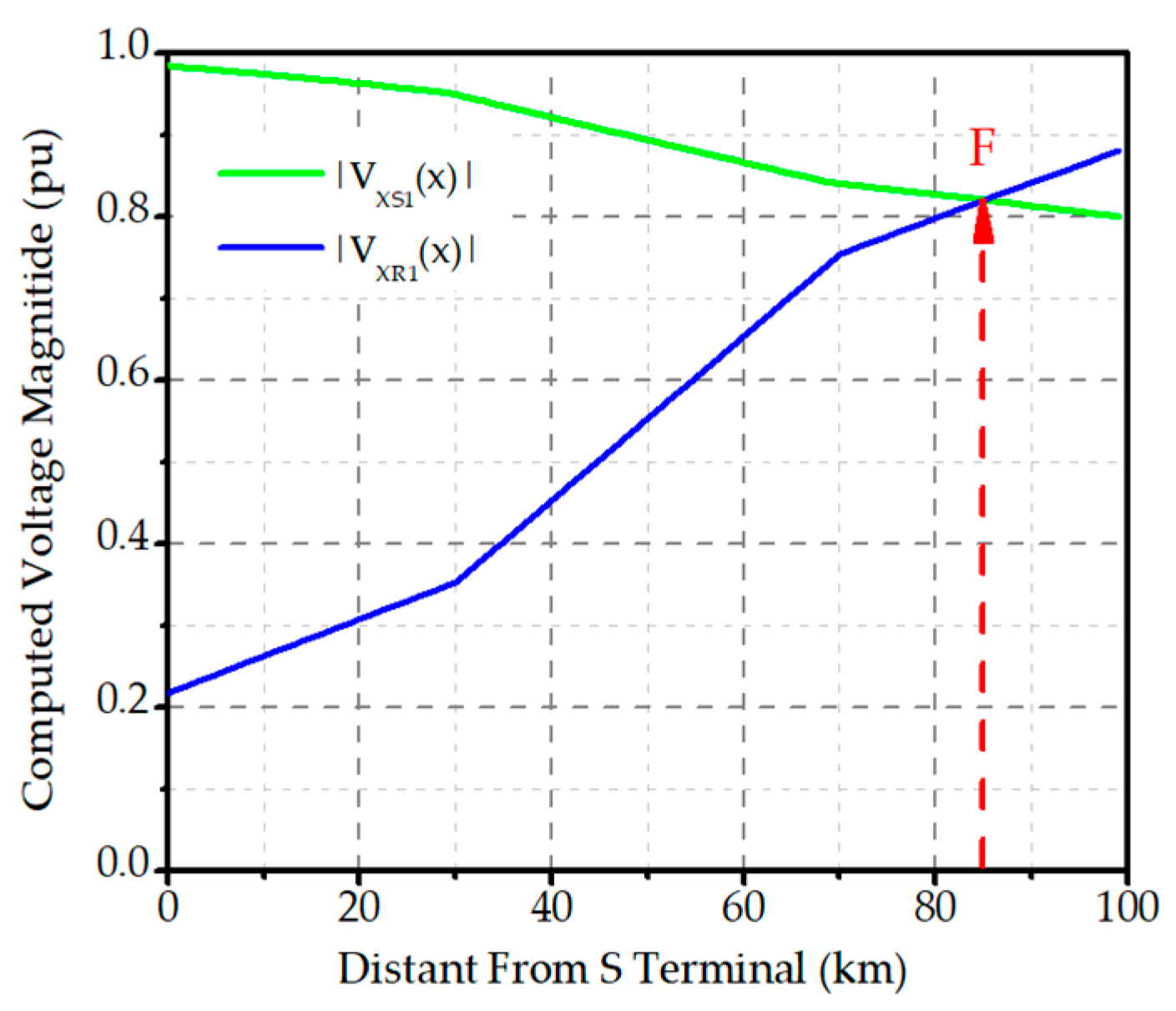
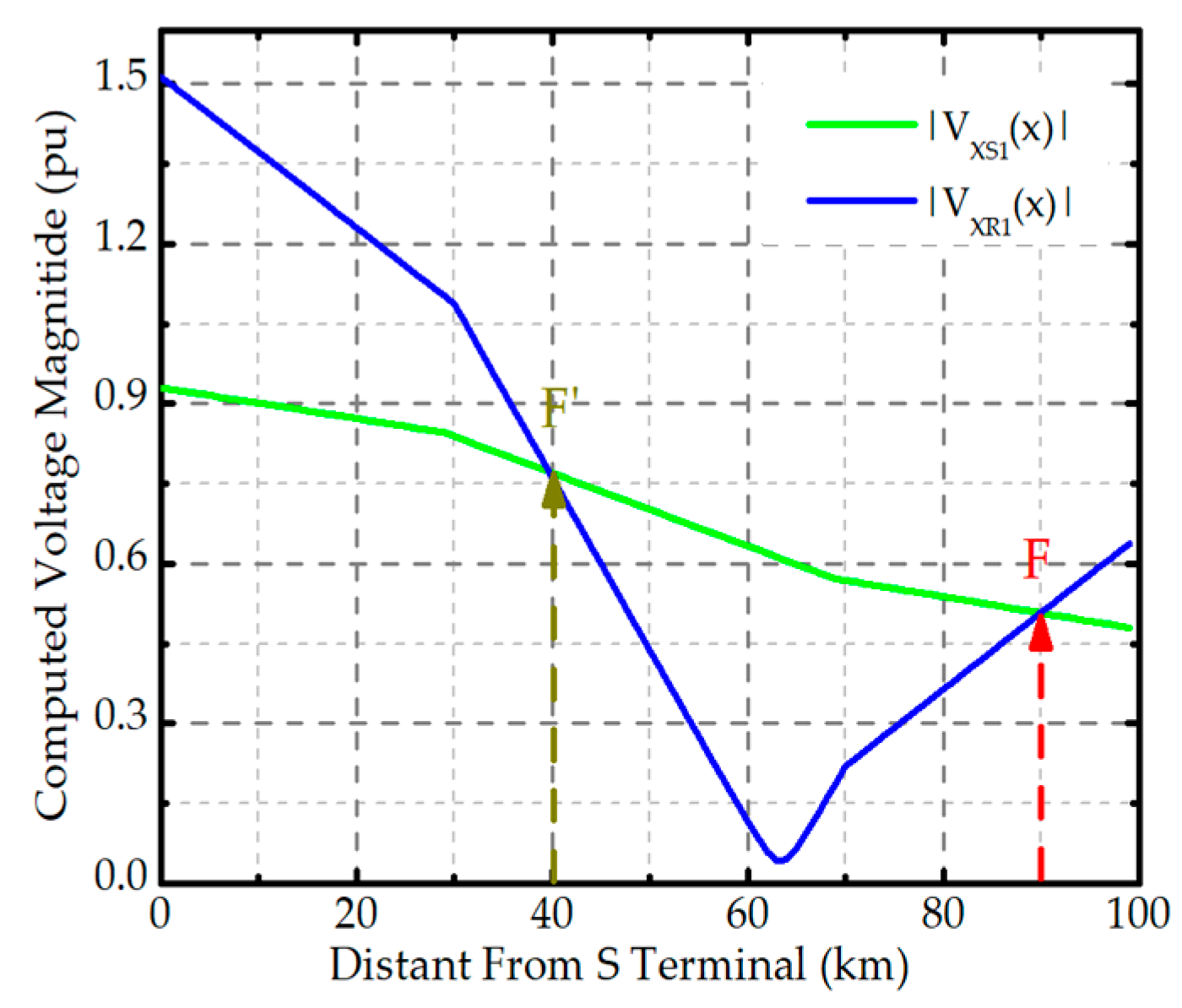
2.3. The Voltage Magnitude Intersection Points

As explained in the previous section, the voltage and current at a given point along the transmission line can be computed using the voltages and currents measured at the terminals with constant line parameters. Figure 3 indicates the magnitude of the computed voltage at various points along a three-section combined transmission line; these are derived from the data obtained at both terminals. At the fault locations, the magnitude of the computed voltage (${\mathrm{V}}_{\mathrm{XS}1}$, ${\mathrm{V}}_{\mathrm{XR}1}$) is identical. This can be written as:

$$\left|{\mathrm{V}}_{\mathrm{XS}1}(\mathrm{F})\right|=\left|{\mathrm{V}}_{\mathrm{XR}1}(\mathrm{F})\right|,$$

(9)

A point F on the transmission line that satisfies (9) is identified as a fault point. The algorithm commences by setting the initial location, x, to zero and subsequently determines the differences [the d(x) values] between the computed voltage magnitudes based on the measurements from both terminals. The calculation proceeds as follows in Equation (10):

$$\mathrm{d}(\mathrm{x})=\left|\left|{\mathrm{V}}_{\mathrm{XS}1}(\mathrm{x})\right|-\left|{\mathrm{V}}_{\mathrm{XR}1}(\mathrm{x})\right|\right|,$$

(10)

As combined transmission lines are inhomogeneous, fault point localization becomes challenging when employing the Newton–Raphson or modified secant method. We use an incremental increase method. Figure 3 indicates that the different value d(x) decreases as x moves closer to the intersection point. Therefore, the algorithm increases x as follows:

x = x + αd(x),

(11)

In order to generalize the increasing rate α to be applicable to different systems, the algorithm is conducted based on the per unit quantity. After evaluation with different values, the increasing rate in Appendix A was selected based on a balance between the convergence speed and accuracy.

This process continues until d(x) converges to the selected perturbation value δ, indicating that Equation (9) is proximity-satisfied. However, if the algorithm cannot find the intersection point (x exceeds 1 or the iteration number attains the maximum threshold), the result at the previous sample will be used instead.

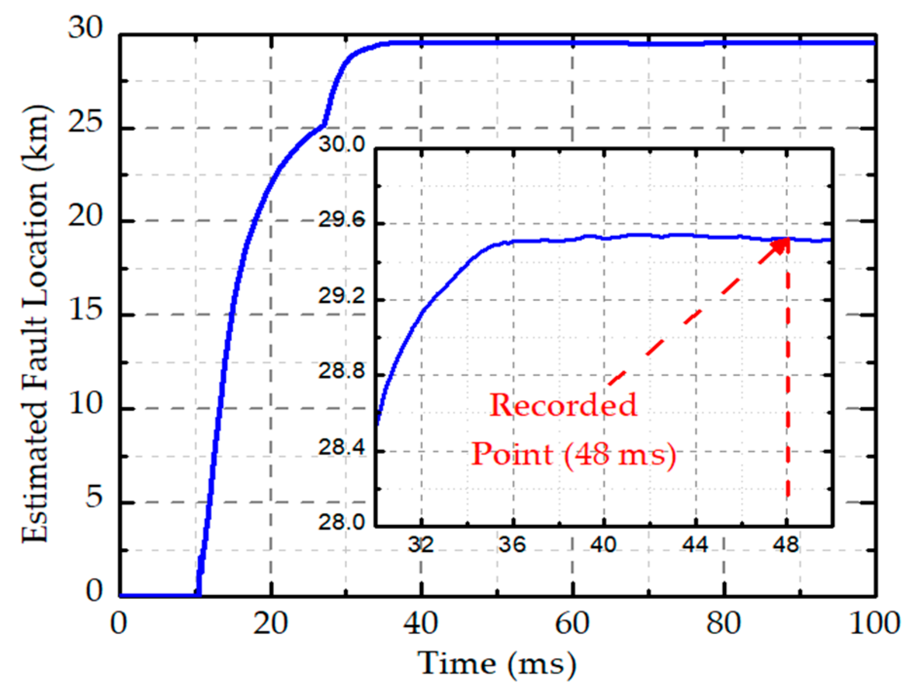
2.4. Real Fault Localization

If a fault occurs on a transmission line, all fault-crossing computations render either Equation (1) or (2) inaccurate, the exception being when the computation point is precisely aligned with the fault location F. This error can introduce a problem that leads to the satisfaction of Equation (9) at a point F’ other than the real fault location F, as illustrated in Figure 4. The consequence is the potential misidentification of the real fault location; a more accurate fault location identification algorithm is imperative.

To address this issue, this paper introduces a novel fault location identification algorithm based on the inverse angle of the equivalent impedance. This leverages insights into the inverse angle that enhance the precision and reliability of the fault localization. By integrating this algorithm into the iterative algorithm discussed in the previous section, spurious fault locations are systematically rejected, and the value of x is incrementally adjusted until the true fault location F is identified.

Figure 5a shows the interconnections between the sequence networks for single-phase-to-ground faults on the transmission line. Z_S0, Z_R0, Z_S1, Z_R1, Z_S2, and Z_R2 are the zero-positive- and zero-negative-sequence sending-end and receiving-end source impedances, respectively. Similarly, Z_LS0, Z_LR0, Z_LS1, Z_LR1, Z_LS2, and Z_LR2 are the zero-positive- and zero-negative-sequence transmission line impedances on the sending-end and receiving-end sides. V_S and V_R are the sending-end and receiving-end voltages and R_F the fault resistance. Figure 5b–d show the interconnections of the sequence networks for phase-to-phase, phase-to-phase-to-ground, and three-phase faults on the transmission line, respectively. From each network in Figure 5, the simplified network in Figure 6 can be derived.

Where Z_eq, the equivalent impedance, varies by the specific type of fault. Despite the distinctive characteristics of the fault types, all Z_eq values are inductive in nature. Using the equivalent network of Figure 6, the equivalent impedance Z_eq can be calculated as:

$${\mathrm{Z}}_{\mathrm{eq}}=\frac{{\mathrm{V}}_{\mathrm{F}}}{{\mathrm{I}}_{\mathrm{F}}},$$

(12)

where ${\mathrm{V}}_{\mathrm{F}}$ and ${\mathrm{I}}_{\mathrm{F}}$ are the positive-sequence voltage and current at the fault point. The phasor quantities can be computed using Equations (13) and (14), respectively:

$${\mathrm{V}}_{\mathrm{F}}={\mathrm{V}}_{\mathrm{XS}1}(\mathrm{x}),$$

(13)

$${\mathrm{I}}_{\mathrm{F}}={\mathrm{I}}_{\mathrm{XS}1}(\mathrm{F})+{\mathrm{I}}_{\mathrm{XR}1}(\mathrm{F})\times \frac{{\mathrm{V}}_{\mathrm{XS}1}(\mathrm{x})}{\left|{\mathrm{V}}_{\mathrm{XS}1}(\mathrm{x})\right|},$$

(14)

Finally, the inverse angle of the equivalent impedance ${\mathsf{\phi }}_{\mathrm{IEZ}}$ can be derived as:

$${\mathsf{\phi }}_{\mathrm{IEZ}}(\mathrm{x})=\mathrm{ang}\left(\left({\mathrm{I}}_{\mathrm{XS}1}(\mathrm{x}) +{\mathrm{I}}_{\mathrm{XR}1}(\mathrm{x}) \times \frac{{\mathrm{V}}_{\mathrm{XS}1}(\mathrm{x})}{\left|{\mathrm{V}}_{\mathrm{XS}1}(\mathrm{x})\right|}\right)\times { {\mathrm{V}}^{\prime }}_{\mathrm{XS}1}(\mathrm{x})\right),$$

(15)

where V′_XS1(x) is the complex conjugate of V_XS1(x) and ang() is the angle computation operator for the phasor quantity.

The inherently inductive characteristics of the equivalent impedance specifically position the inverse phase angle ${\mathsf{\phi }}_{\mathrm{IEZ}}$ on the complex plane. When the distance x yielded by the iterative method of the above section is an actual fault location, the inverse phase angle ${\mathsf{\phi }}_{\mathrm{IEZ}}$ falls within the fourth quadrant. Conversely, if x is not the location of a real fault, ${\mathsf{\phi }}_{\mathrm{IEZ}}$ lies outside the fourth quadrant. This distinctive behavior distinguishes real from misidentified faults. By analyzing the locations of the inverse phase angles on the complex plane, the misidentified fault locations reported by the voltage magnitude intersection point algorithm are rejected until the actual fault is identified.

The flowchart of our new fault location algorithm for combined transmission lines wherein sampling is unsynchronized is shown in Figure 7.

3. Simulation Results and Performance Evaluation

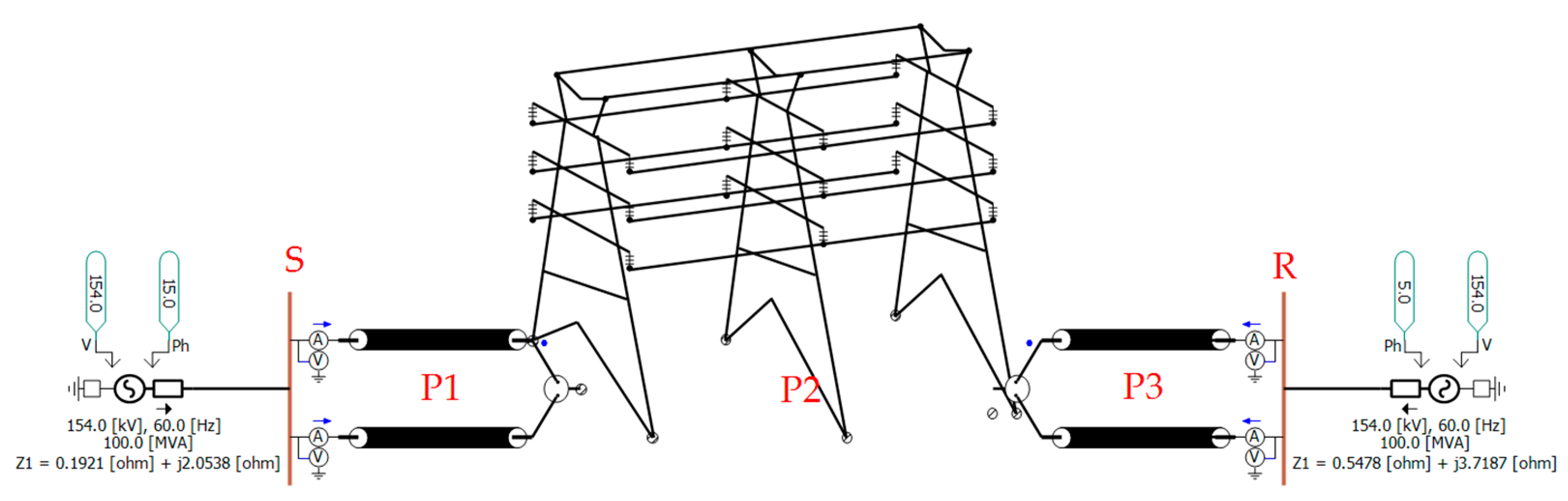
3.1. The Test Environment

To evaluate the performance of the presented technique, the 154 kV double-circuit, three-section combined transmission line shown in Figure 8 was simulated with the aid of PSCAD/EMTDC. The line is segmented into three parts: P1, P2, and P3. P1 and P3 are both 3-km long double-circuit underground cables; P2 is a 40 km long double-circuit overhead transmission line between P1 and P3. Overhead line transposition and underground cable cross-bonding were considered during the testing. The detailed model parameters can be found in Appendix B.

The double circuit was considered to be two independent single circuits; the new fault location technique could thus be applied to each line individually. The algorithm was implemented employing the user-defined model of PSCAD/EMTDC. The sampling frequency was 4800 Hz or 80 samples/cycle; the fundamental frequency was 60 Hz. The method of [35] was used to remove the decaying DC offset and to derive the fundamental phasors of each measured signal. The performance of the algorithm was assessed based on the error percentage:

$$\mathrm{E}\mathrm{r}\mathrm{r}\mathrm{o}\mathrm{r}(\mathrm{\%})=\frac{\left|\mathrm{Estimated} \mathrm{Fault} \mathrm{Location} - \mathrm{Actual} \mathrm{Fault} \mathrm{Location}\right|}{\mathrm{Total} \mathrm{Transmission} \mathrm{Line} \mathrm{Length}},$$

(16)

3.2. Case Studies

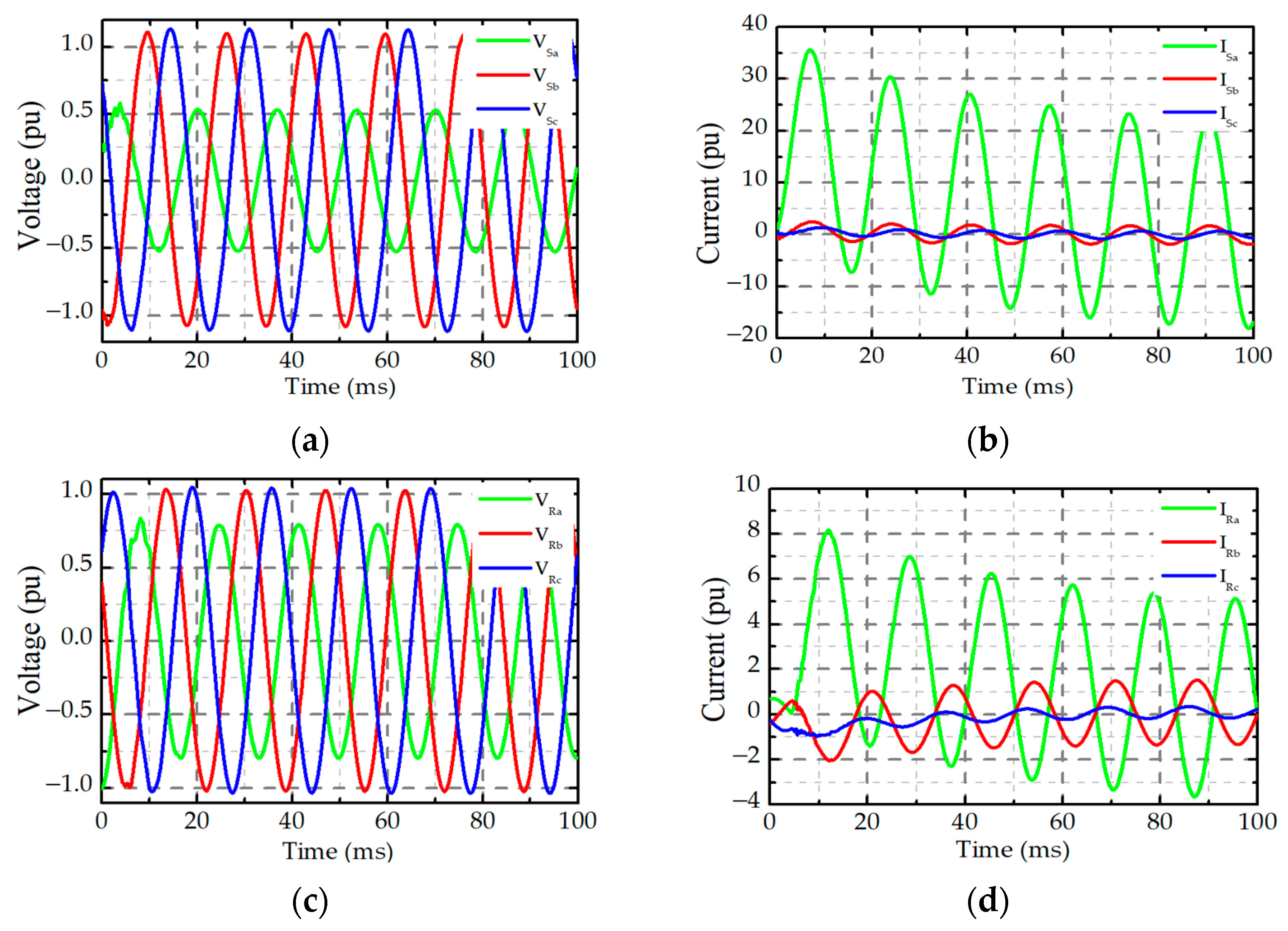
3.2.1. Influence of the Phasor Synchronization Error and Fault Types

Several simulations were performed using the new algorithm. We varied the fault types and resistance and the phasor synchronization errors. For example, Figure 9 shows the three-phase voltages and currents recorded at the S and R terminals assuming a single-phase-to-ground fault occurs at a 29.5 km distance from the S bus in the cable section, thus very close to the connection to the overhead transmission line (and the fault resistance is therefore 0 Ω). The phase error between the data recorded at both terminals is 90°.

By applying the presented approach with constrained parameters in Appendix A to the fault-recorded data in Figure 9, the estimated fault location result in Figure 10 is provided. It is evident in Figure 10 that the proposed algorithm is applicable for estimating the fault location on a multi-section combined transmission line with an acceptable convergence time, even though the recorded data from both terminals are not synchronized. The estimation error falls to below 1% within the first two cycles of the fault. After three cycles, the estimated error is 0.015%, corresponding to a common protective relay tripping time.

The full test results using single-phase-to-ground faults with different fault resistances and phasor synchronization angle errors are shown in

Table 2. Test data on single-phase-to-ground faults at different locations along the transmission line with variation in the fault resistance and phase errors.

Fault Resistance	Phase Error	10 km (P1)		50 km (P2)		80 km (P3)
(Ω)	(°)	Location (km)	Error (%)	Location (km)	Error (%)	Location (km)	Error (%)
0	0	9.992	0.008	49.995	0.005	79.976	0.024
	30	9.994	0.006	49.996	0.004	79.980	0.020
	60	9.995	0.005	49.995	0.005	79.984	0.016
	90	10.002	0.002	49.995	0.005	79.972	0.028
	180	10.023	0.023	50.012	0.012	79.996	0.004
30	0	9.656	0.344	49.859	0.141	79.668	0.332
	30	9.788	0.212	49.904	0.096	79.783	0.217
	60	9.930	0.070	49.891	0.109	79.886	0.114
	90	10.031	0.031	49.984	0.016	80.282	0.282
	180	10.468	0.468	50.135	0.135	79.902	0.098
50	0	9.310	0.690	49.686	0.314	79.401	0.599
	30	9.553	0.447	49.787	0.213	79.601	0.399
	60	9.836	0.164	49.892	0.108	79.813	0.187
	90	10.034	0.034	50.019	0.019	79.992	0.008
	180	9.378	0.623	50.381	0.381	79.683	0.317

. The fault resistance ranged from 0 to 50 Ω and the phasor synchronization error from 0 to 180°. Three different faults at distances of 10, 50, and 80 km from terminal S were created on the combined transmission line. The estimated fault locations were captured three cycles after the fault initialization. The estimation errors listed in Table 2 show that the errors for the same fault resistances were very similar, although the phasor synchronization angle errors and fault locations differed. This indicates that the algorithm is accurate; it is not affected by phasor synchronization errors. The smallest estimation error was less than 0.002% for a single-phase-to-ground fault with a fault resistance of 0 Ω 10 km from the S terminal. Although the estimation error increases as the fault resistance rises, the maximum error was only 0.623% for a single-phase-to-ground fault with a resistance of 50 Ω 10 km from the S terminal. Other fault locations exhibited the same lowest errors (0.004%) for 0 Ω fault resistances. The highest errors were 0.381 and 0.599% for fault resistances of 50 Ω 50 and 80 km from the S terminal, respectively. The fault resistance more significantly affects faults in underground cables than faults in overhead transmission lines, reflecting the effects of cross-bonding on fault location algorithms.

Testing was next expanded to include phase-to-phase, phase-to-phase-to-ground, and three-phase faults; we comprehensively evaluated how the new algorithm performed under various fault scenarios. The conditions used during the single-phase-to-ground fault tests were maintained (to ensure consistency).

Table 3. Test results for phase-to-phase faults at different locations along the transmission line with variation in the fault resistance and phase errors.

Fault Resistance	Phase Error	10 km (P1)		50 km (P2)		80 km (P3)
(Ω)	(°)	Location (km)	Error (%)	Location (km)	Error (%)	Location (km)	Error (%)
0	0	9.995	0.005	50.018	0.018	79.992	0.008
	30	10.009	0.009	50.018	0.018	79.991	0.009
	60	10.013	0.013	50.019	0.019	79.990	0.010
	90	10.019	0.019	50.020	0.020	79.994	0.006
	180	10.043	0.043	50.024	0.024	80.003	0.003
30	0	9.703	0.297	50.060	0.060	79.953	0.047
	30	9.775	0.225	50.096	0.096	80.017	0.017
	60	9.877	0.123	50.129	0.129	80.085	0.085
	90	9.919	0.081	50.144	0.144	80.139	0.139
	180	10.194	0.194	50.276	0.276	80.363	0.363
50	0	9.605	0.395	49.981	0.019	79.939	0.061
	30	9.771	0.229	50.050	0.050	80.064	0.064
	60	9.955	0.045	50.137	0.137	80.202	0.202
	90	10.020	0.020	50.171	0.171	80.315	0.315
	180	10.495	0.495	50.458	0.458	80.757	0.757

shows the performance of the algorithm when phase-to-phase faults develop. The estimation errors at different phase synchronization angle errors but at the same fault resistance are similar; however, the difference increases at higher fault resistances. The error variations at the various fault locations are similar. Specifically, the minimum estimation errors for faults at distances of 10, 50, and 80 km from the S terminal were 0.005, 0.018, and 0.003% and the maximum errors 0.495, 0.458, and 0.757%, respectively.

Table 4. Test results for phase-to-phase-to-ground faults at different locations along the transmission line with variation in the fault resistance and phase errors.

Fault Resistance	Phase Error	10 km (P1)		50 km (P2)		80 km (P3)
(Ω)	(°)	Location (km)	Error (%)	Location (km)	Error (%)	Location (km)	Error (%)
0	0	10.001	0.001	50.013	0.013	79.994	0.006
	30	10.020	0.020	50.014	0.014	79.998	0.002
	60	10.014	0.014	50.015	0.015	79.998	0.002
	90	10.016	0.016	50.016	0.016	79.998	0.002
	180	9.984	0.016	50.013	0.013	79.996	0.004
30	0	10.004	0.004	50.062	0.062	79.857	0.143
	30	10.052	0.052	50.077	0.077	79.890	0.110
	60	10.094	0.094	50.092	0.092	79.924	0.076
	90	10.125	0.125	50.105	0.105	79.955	0.045
	180	10.243	0.243	50.177	0.177	80.047	0.047
50	0	10.005	0.005	50.028	0.028	79.765	0.235
	30	10.086	0.086	50.061	0.061	79.832	0.168
	60	10.197	0.197	50.095	0.095	79.902	0.098
	90	10.233	0.233	50.124	0.124	79.963	0.037
	180	10.477	0.477	50.246	0.246	80.176	0.176

shows that the new algorithm performs well when phase-to-phase-to-ground faults develop under the described conditions. The algorithm accurately locates the faults; the minimum and maximum errors are 0.001 and 0.477%.

The response of the proposed algorithm to three-phase faults is shown in

Table 5. Test results for three-phase faults at different locations along the transmission line with variation in the fault resistance and phase errors.

Fault Resistance	Phase Error	10 km (P1)		50 km (P2)		80 km (P3)
(Ω)	(°)	Location (km)	Error (%)	Location (km)	Error (%)	Location (km)	Error (%)
0	0	9.816	0.184	49.697	0.303	80.112	0.112
	30	9.801	0.199	49.750	0.250	80.114	0.114
	60	9.791	0.209	49.753	0.247	80.113	0.113
	90	9.777	0.223	49.626	0.374	80.118	0.118
	180	9.721	0.279	49.458	0.542	80.118	0.118
30	0	9.845	0.155	49.846	0.154	79.731	0.269
	30	9.915	0.085	49.900	0.100	79.801	0.199
	60	9.989	0.011	49.961	0.039	79.869	0.131
	90	10.039	0.039	49.965	0.035	79.931	0.069
	180	10.235	0.235	50.207	0.207	80.188	0.188
50	0	9.710	0.290	49.705	0.295	79.610	0.390
	30	9.810	0.190	49.820	0.180	79.726	0.274
	60	9.958	0.042	49.943	0.057	79.847	0.153
	90	10.028	0.028	50.016	0.016	79.953	0.047
	180	10.334	0.334	50.372	0.372	80.362	0.362

. For a fault resistance of 0 Ω, a noticeable error (0.542%) occurs at the 50 km point of the overhead line when the input phase error is 180. As the fault resistance increases, the error becomes insignificant compared to the previous cases.

3.2.2. Influence of Fault Inception Angles

The proposed algorithm was also verified under various fault inception angles. In this case, single-phase-to-ground faults with different fault resistances and locations were simulated with fault inception angles varying from 0 to 180°. The testing results in

Table 6. Test results for single-phase-to-ground faults at different locations along the transmission line. The fault resistances and fault inception angles varied.

Fault Resistance	Fault Inception Angle	10 km (P1)		50 km (P2)		80 km (P3)
(Ω)	(°)	Location (km)	Error (%)	Location (km)	Error (%)	Location (km)	Error (%)
0	0	10.012	0.012	49.984	0.016	79.958	0.042
	30	9.970	0.030	49.991	0.009	79.958	0.042
	60	9.951	0.049	49.885	0.115	79.993	0.007
	90	9.938	0.062	49.974	0.026	79.862	0.138
	180	9.988	0.012	50.008	0.008	80.032	0.032
30	0	9.668	0.332	49.860	0.140	79.677	0.323
	30	9.419	0.581	49.946	0.054	79.411	0.589
	60	9.901	0.099	49.970	0.030	79.483	0.517
	90	10.027	0.027	49.906	0.094	79.803	0.197
	180	9.627	0.373	49.618	0.382	79.763	0.237
50	0	9.351	0.649	49.711	0.289	79.396	0.604
	30	9.171	0.829	49.753	0.247	79.533	0.467
	60	9.417	0.583	49.532	0.468	79.582	0.418
	90	9.417	0.583	49.596	0.404	79.495	0.505
	180	9.179	0.821	49.685	0.315	80.362	0.362

indicate that the proposed algorithm remains effective and unaffected by variation in the fault inception angles.

3.2.3. Influence of Source Impedance Variation

Moreover, the algorithm reliability was assessed by varying the source impedance.

Table 7. Test results for single-phase-to-ground faults along the transmission line. The source impedance varied.

Source S				Source R				10 km		50 km
Positive		Zero		Positive		Zero
R1	X1	R0	X0	R1	X1	R0	X0	Location (km)	Error (%)	Location (km)	Error (%)
(Ω)		(Ω)		(Ω)		(Ω)
0.1729	1.8484	0.8196	4.1749	0.4930	3.3468	2.0042	9.7779	10.135	0.135	49.983	0.017
0.2113	2.2592	1.0018	5.1027	0.6026	4.0906	2.4496	11.9507	10.105	0.105	50.001	0.001

demonstrates the test results for single-phase-to-ground faults at different locations along the transmission line with 0 Ω fault resistance. It can be seen that the proposed algorithm can estimate the fault location accurately with different source impedances.

3.2.4. Comparison of the Proposed Algorithm with the Algorithm in [31]

A comparison between the proposed algorithm and the algorithm in [31] is shown in

Table 8. Comparison results for single-phase-to-ground faults at different locations along the transmission line. The fault resistances and fault inception angles varied.

Fault Types	Fault Location	Proposed Algorithm		Algorithm in [31]
	(km)	Location (km)	Error (%)	Location (km)	Error (%)
Single-phase-to-ground	10	9.931	0.069	10.124	0.124
	50	49.991	0.009	49.992	0.008
	80	79.947	0.053	80.005	0.005
Phase-to-phase	10	9.845	0.155	10.253	0.253
	50	49.860	0.140	50.092	0.092
	80	79.783	0.217	79.857	0.143
Phase-to-phase-to ground	10	9.982	0.018	09.832	0.168
	50	49.970	0.030	50.020	0.020
	80	79.936	0.064	79.927	0.073
Three-phase	10	9.489	0.511	10.006	0.006
	50	49.499	0.501	49.987	0.013
	80	80.294	0.294	80.154	0.154

, which shows the estimation results and percentage error for different types of faults, a 10 Ω fault resistance, a 0° synchronous angle (synchronous measurements), and different fault locations. As seen from Table 8, the proposed algorithm achieves a similar accuracy compared to the algorithm in [31]. While the proposed algorithm may have a slower calculation speed, it is capable of handling unsynchronized sampling, a feature the algorithm presented in [31] lacks.

4. Conclusions

This paper presents a novel fault location estimation algorithm for a multi-section combined transmission line considering unsynchronized sampling. After the fault is detected, the fault waveforms for both terminals are collected. The proposed algorithm uses the voltage and current data to compute the voltage magnitudes at a specific point along the transmission line and subsequently compares them. If the magnitudes are found to be equal, the specific point is recognized as the intersection point. In cases of different magnitudes, the computation point is adjusted, and the process is iterated. Once an intersection point is determined, fault location identification is applied to check whether it is a valid fault. If not, the process moves to another point; otherwise, the fault location estimation process is considered complete. The simulation results show that the proposed algorithm was robust across various fault types and phase synchronization errors regardless of variation in the fault inception angle, fault resistance, and source impedance. The algorithm is practical; no more than three cycles of fault data are required.

As future work, the performance of proposed algorithm under nonlinear faults will be evaluated. Additionally, we plan to optimize the detection of the voltage magnitude intersection points to increase the effectiveness of the algorithm; thus, the algorithm will be suitable for online applications.

References

1. IEEE Std C37.114-2004; IEEE Guide for Determining Fault Location on AC Transmission and Distribution Lines. IEEE Power Engineering Society: Piscataway, NJ, USA, 2005; pp. 1–44.
2. Mazon, A.J.; Zamora, I.; Miñambres, J.F.; Zorrozua, M.A.; Barandiaran, J.J.; Sagastabeitia, K. A new approach to fault location in two-terminal transmission lines using artificial neural networks. Electr. Power Syst. Res. 2000, 56, 261–266. [Google Scholar] [CrossRef]
3. Rocha, S.A.; Mattos, T.G.; Cardoso, R.T.N.; Silveira, E.G. Applying Artificial Neural Networks and Nonlinear Optimization Techniques to Fault Location in Transmission Lines—Statistical Analysis. Energies 2022, 15, 4095. [Google Scholar] [CrossRef]
4. Stanojević, V.A.; Preston, G.; Terzija, V. Synchronised Measurements Based Algorithm for Long Transmission Line Fault Analysis. IEEE Trans. Smart Grid 2018, 9, 4448–4457. [Google Scholar] [CrossRef]
5. Kalita, K.; Anand, S.; Parida, S.K. A Novel Non-Iterative Fault Location Algorithm for Transmission Line With Unsynchronized Terminal. IEEE Trans. Power Deliv. 2021, 36, 1917–1920. [Google Scholar] [CrossRef]
6. Naidu, O.; Pradhan, A.K. A Traveling Wave-Based Fault Location Method Using Unsynchronized Current Measurements. IEEE Trans. Power Deliv. 2019, 34, 505–513. [Google Scholar] [CrossRef]
7. Carrión, D.; González, J.W.; Issac, I.A.; López, G.J. Optimal fault location in transmission lines using hybrid method. In Proceedings of the 2017 IEEE PES Innovative Smart Grid Technologies Conference—Latin America (ISGT Latin America), Quito, Ecuador, 20–22 September 2017. [Google Scholar]
8. Elnozahy, A.; Sayed, K.; Bahyeldin, M. Artificial Neural Network Based Fault Classification and Location for Transmission Lines. In Proceedings of the 2019 IEEE Conference on Power Electronics and Renewable Energy (CPERE), Aswan, Egypt, 23–25 October 2019. [Google Scholar]
9. Fahim, S.R.; Sarker, Y.; Islam, O.K.; Sarker, S.K.; Ishraque, M.F.; Das, S.K. An Intelligent Approach of Fault Classification and Localization of a Power Transmission Line. In Proceedings of the 2019 IEEE International Conference on Power, Electrical, and Electronics and Industrial Applications (PEEIACON), Dhaka, Bangladesh, 29 November–1 December 2019. [Google Scholar]
10. Livani, H.; Evrenosoglu, C.Y. A Machine Learning and Wavelet-Based Fault Location Method for Hybrid Transmission Lines. IEEE Trans. Smart Grid 2014, 5, 51–59. [Google Scholar] [CrossRef]
11. Sadeh, J.; Afradi, H. A new and accurate fault location algorithm for combined transmission lines using Adaptive Network-Based Fuzzy Inference System. Electr. Power Syst. Res. 2009, 79, 1538–1545. [Google Scholar] [CrossRef]
12. Patel, B. A new FDOST entropy based intelligent digital relaying for detection, classification and localization of faults on the hybrid transmission line. Electr. Power Syst. Res. 2018, 157, 39–47. [Google Scholar] [CrossRef]
13. Abur, A.; Magnago, F.H. Use of time delays between modal components in wavelet based fault location. Int. J. Electr. Power Energy Syst. 2000, 22, 397–403. [Google Scholar] [CrossRef]
14. Faybisovich, V.; Khoroshev, M.I. A Frequency domain double-ended method of fault location for transmission lines. In Proceedings of the 2008 IEEE/PES Transmission and Distribution Conference and Exposition, Chicago, IL, USA, 21–24 April 2008. [Google Scholar]
15. Styvaktakis, E.; Bollen, M.H.J.; Gu, I.Y.H. A fault location technique using high frequency fault clearing transients. IEEE Power Eng. Rev. 1999, 19, 58–60. [Google Scholar] [CrossRef]
16. Gilany, M.I.; Tag Eldin, E.S.M.; Abdel Aziz, M.M.; Ibrahim, D.K. Travelling Wave-Based Fault Location Scheme for Aged Underground Cable Combined with Overhead Line. Int. J. Emerg. Electr. 2005, 2. [Google Scholar] [CrossRef]
17. Li, Y.; Zhang, Y.; Ma, Z. Fault location method based on the periodicity of the transient voltage traveling wave. In Proceedings of the 2004 IEEE Region 10 Conference TENCON 2004, Chiang Mai, Thailand, 24 November 2004. [Google Scholar]
18. Jung, C.K.; Lee, J.B. Fault Location Using Wavelet Transform in Combined Transmission Systems. IFAC Proc. Vol. 2003, 36, 617–622. [Google Scholar] [CrossRef]
19. Niazy, I.; Sadeh, J. A new single ended fault location algorithm for combined transmission line considering fault clearing transients without using line parameters. Int. J. Electr. Power Energy Syst. 2013, 44, 816–823. [Google Scholar] [CrossRef]
20. Takagi, T.; Yamakoshi, Y.; Baba, J.; Uemura, K.; Sakaguchi, T. A New Algorithm of an Accurate Fault Location for EHV/UHV Transmission Lines: Part II—Laplace Transform Method. IEEE Trans. Power App. Syst. 1982, PAS-101, 564–573. [Google Scholar] [CrossRef]
21. Takagi, T.; Yamakoshi, Y.; Yamaura, M.; Kondow, R.; Matsushima, T. Development of a New Type Fault Locator Using the One-Terminal Voltage and Current Data. IEEE Trans. Power App. Syst. 1982, PER-2, 59–60. [Google Scholar]
22. Zahran, A.D.; Elkalashy, N.I.; Elsadd, M.A.; Kawady, T.A.; Taalab, A.-M.I. Improved ground distance protection for cascaded overhead-submarine cable transmission system. In Proceedings of the 2017 Nineteenth International Middle East Power Systems Conference (MEPCON), Cairo, Egypt, 19–21 December 2017. [Google Scholar]
23. Bukvisova, Z.; Orsagova, J.; Topolanek, D.; Toman, P. Two-Terminal Algorithm Analysis for Unsymmetrical Fault Location on 110 kV Lines. Energies 2019, 12, 1193. [Google Scholar] [CrossRef]
24. Kezunović, M.; Mrkić, J.; Peruničić, B. An accurate fault location algorithm using synchronized sampling. Electr. Power Syst. Res. 1994, 29, 161–169. [Google Scholar] [CrossRef]
25. Kezunovic, M.; Perunicic, B. Automated transmission line fault analysis using synchronized sampling at two ends. IEEE Trans. Power Syst. 1996, 11, 441–447. [Google Scholar] [CrossRef]
26. Dalcastagne, A.L.; Filho, S.N.; Zurn, H.H.; Seara, R. An Iterative Two-Terminal Fault-Location Method Based on Unsynchronized Phasors. IEEE Trans. Power Deliv. 2008, 23, 2318–2329. [Google Scholar] [CrossRef]
27. Yu, C.-S. An Unsynchronized Measurements Correction Method for Two-Terminal Fault-Location Problems. IEEE Trans. Power Deliv. 2010, 25, 1325–1333. [Google Scholar] [CrossRef]
28. Elsadd, M.A.; Abdelaziz, A.Y. Unsynchronized fault-location technique for two- and three-terminal transmission lines. Electr. Power Syst. Res. 2018, 158, 228–239. [Google Scholar] [CrossRef]
29. Lin, T.C.; Xu, Z.R.; Ouedraogo, F.B.; Lee, Y.J. A new fault location technique for three-terminal transmission grids using unsynchronized sampling. Int. J. Electr. Power Energy Syst. 2020, 123, 106229. [Google Scholar] [CrossRef]
30. Aziz, M.M.A.; Khalil Ibrahim, D.; Gilany, M. Fault location scheme for combined overhead line with underground power cable. Electr. Power Syst. Res. 2006, 76, 928–935. [Google Scholar]
31. Liu, C.-W.; Lin, T.-C.; Yu, C.-S.; Yang, J.-Z. A Fault Location Technique for Two-Terminal Multisection Compound Transmission Lines Using Synchronized Phasor Measurements. IEEE Trans. Smart Grid 2012, 3, 113–121. [Google Scholar] [CrossRef]
32. Elsadd, M.A.; Omar, H.A.; Adly, A.R.; Zobaa, A.F. Fault-Locator Scheme for Combined Taba-Aqaba Transmission System Based on New Faulted Segment Identification Method. IEEE Access 2023, 11, 104270–104284. [Google Scholar] [CrossRef]
33. Hashemian, S.M.; Hashemian, S.N.; Gholipour, M. Unsynchronized parameter free fault location scheme for hybrid transmission line. Electr. Power Syst. Res. 2021, 192, 106982. [Google Scholar] [CrossRef]
34. Jiang, J.A.; Yang, J.Z.; Lin, Y.H.; Liu, C.W.; Ma, J.C. An adaptive PMU based fault detection/location technique for transmission lines. I. IEEE Trans. Power Deliv. 2000, 15, 486–493. [Google Scholar] [CrossRef]
35. Guo, Y.; Kezunovic, M.; Chen, D. Simplified algorithms for removal of the effect of exponentially decaying DC-offset on the Fourier algorithm. IEEE Trans. Power Deliv. 2003, 18, 711–717. [Google Scholar]
Figure 1. A single-line diagram of a homogenous transmission line.
Energies 17 00703 g001
Figure 2. A single-line diagram of a three-section combined transmission line.
Energies 17 00703 g002
Figure 3. Computed voltage magnitudes along the transmission line based on the S and R terminal fault record data.
Energies 17 00703 g003
Figure 4. Computed voltage magnitudes along a transmission line based on S and R terminal fault record data when there are two intersection points.
Energies 17 00703 g004
Figure 5. Interconnections among the sequence networks for (a) a single-phase-to-ground fault; (b) a phase-to-phase fault; (c) a phase-to-phase-to-ground fault; and (d) a three-phase fault.
Energies 17 00703 g005
Figure 6. Equivalent interconnection network for different types of faults.
Energies 17 00703 g006
Figure 7. Flowchart of the fault location algorithm.
Energies 17 00703 g007
Figure 8. PSCAD/EMTDC three-section combined transmission line model.
Energies 17 00703 g008
Figure 9. Single-phase-to-ground fault records of (a) the voltage at the S terminal; (b) the current at the S terminal; (c) the voltage at the R terminal; (d) the current at the R terminal.
Energies 17 00703 g009
Figure 10. Localization of a single-phase-to-ground fault at 29.5 km distance from the S terminal.
Energies 17 00703 g010