Article

Modeling of a Biomass-Based Energy Production Case Study Using Flexible Inputs with the P-Graph Framework

1
Department of Computer Science and Systems Technology, University of Pannonia, 8200 Veszprém, Hungary
2
Department of Applied Sustainability, Albert Kázmér Faculty of Agricultural and Food Sciences, Széchenyi István University of Győr, 9026 Győr, Hungary
*
Author to whom correspondence should be addressed.
Energies 2024, 17(3), 687; https://doi.org/10.3390/en17030687
Submission received: 19 November 2023 / Revised: 17 January 2024 / Accepted: 26 January 2024 / Published: 31 January 2024
(This article belongs to the Special Issue Advanced Energy Generation Systems for Sustainable Development)

Abstract

:
In this work, a modeling technique utilizing the P-Graph framework was used for a case study involving biomass-based local energy production. In recent years, distributed energy systems gained attention. These systems aim to satisfy energy supply demands, support the local economy, decrease transportation needs and dependence on imports, and, in general, obtain a more sustainable energy production process. Designing such systems is a challenge, for which novel optimization approaches were developed to help decision making. Previous work used the P-Graph framework to optimize energy production in a small rural area, involving manure, intercrops, grass, and corn silage as inputs and fermenters. Biogas is produced in fermenters, and Combined Heat and Power (CHP) plants provide heat and electricity. A more recent result introduced the concept of operations with flexible inputs in the P-Graph framework. In this work, the concept of flexible inputs was applied to model fermenters in the original case study. A new implementation of the original decision problem was made both as a Mixed-Integer Linear Programming (MILP) model and as a purely P-Graph model by using the flexible input technique. Both approaches provided the same optimal solution, with a 31% larger profit than the fixed input model.

1. Introduction

Biomass utilization is increasingly popular due to its capability to decrease dependence on fossil fuels and promote sustainability. Agricultural side products and waste can be used with the appropriate technologies to produce energy, fuels, or other products. In practice, the availability of such types of biomass can be problematic since the supplies are not only scarce but distributed geographically, and seasonally and may also fluctuate [1]. Transportation can also be an issue, as the low energy density of the biomass itself may counter the economical incentive of its usage [2].
For these reasons, it can be a challenge to design production plans or whole supply chains involving biomass. A range of optimization methods, including mathematical programming approaches, metaheuristics, and combinatorial optimization methods, were utilized for these and similar purposes [3].
The P-Graph framework is a graph-based combinatorial modeling and optimization tool. An excellent overview of P-Graphs is given by [4]. A recent result was the technique of modeling operations with so-called flexible inputs [5]. This concept makes it possible to model operations having independent inputs and arbitrary linear constraints. Flexible inputs can be especially useful for modeling different types of biomass, which usually have distinct properties.
The main goal of this study is to provide a new P-Graph model using flexible inputs for solving biomass-based energy production problems, which is, to our best knowledge, unprecedented in the literature. This same problem specification was addressed by an equivalent MILP model formulation as well.
A former case study [6], with additional details in [7], targeted the incorporation of intercrops and other biomass types into biogas-based local heat and electricity production in a rural area. This case study was revisited and its model was reproduced as MILP and P-Graph models. The reason this case study was chosen is that it used a P-Graph model for optimization relying on a fixed input model for fermenter units. Therefore, in this problem instance, we can also demonstrate a comparison between the fixed and flexible input modeling techniques with our new models. This article is a direct continuation of our previous work [8]. In our previous work, we already published the results obtained from the MILP model. There were three steps in the development of the MILP model. These steps were distinguished for the sake of a fair comparison of the modeling techniques, as described later in this work. The final MILP model version uses flexible input fermenters.
Our current work completes the task by introducing a P-Graph model for the same problem specification, using flexible input fermenters. This P-Graph model is equivalent to the MILP model using flexible inputs. For the sake of completeness, both the MILP and P-Graph model formulations are presented here. We hope our models can serve as good starting points for designing more effective models, especially P-Graph approaches, for processes involving multiple inputs.
Since this work relies on a case study involving biomass-based energy production, a brief review is first given for this topic. Afterward, the literature on the P-Graph framework is detailed.

1.1. Biomass-Based Energy Supply

Utilizing the energy content of biomass is becoming more considered for producing heat and electricity, fuels, or other products. Besides being renewable and economically competitive, biomass has the potential to decrease dependence on fossil fuels [9]. Several technologies exist to convert biomass into energy or fuel, including simple combustion, gasification, pyrolysis, fermentation, and anaerobic digestion [10]. Most optimization models aim at either supply chains, involving resource management, transportation, production, and delivery, or only the conversion processes themselves in a single facility.
Due to the low energy density of many types of biomass, especially agricultural residues, biomass densification is an important step to make it economically feasible to be transported from the site of availability to the processing locations [11]. Optimization goals may be profit maximization or cost minimization subject to energy demands. Mathematical programming is a popular approach in designing supply chains [12], but combinations with other tools are also common. Ref. [13] used a Genetic Algorithm (GA) to obtain initial solutions and then mathematical programming for maximizing investment value for arbitrary potential biomass types and facilities. Ref. [14] proposed an MILP model assuming a given set of biomass types and processing locations. Their work accounted for both centralized and distributed process networks, which is another key decision. Some models proposed in the literature attempt to cover optimizing for more general supply chains [15]. A review of further case studies for biomass-based energy supply design was provided by [16]. In general, the computational complexity of a problem does not depend on how large the scope is, e.g., complete countries or a small rural area, but on the granularity of decisions in the model.
The conversion processes of biomass can also be optimized, but the resulting models are usually nonlinear and very complex. One option for this purpose is using mixed-integer nonlinear programming [17]. Some approaches combine mathematical programming with metaheuristics like GA [18]. These two examples focus only on hydrogen and power production. Energy supply optimization may also consider other renewable energy sources simultaneously, for example, solar power [19]. On the other hand, if optimization takes place for a supply chain, individual technologies are often simplified and considered as black box operations. More examples for optimizing biomass-based energy production can be found in [20].

1.2. P-Graph Framework

The Process Graph or P-Graph [21] is a directed bipartite graph used to model Process Network Synthesis (PNS) problems. It has two types of nodes: material nodes, which represent resources, and operating unit nodes, which represent any kind of production, transformation, transportation, or conversion from a set of input resources into a set of outputs. The solution structure of a P-Graph is a subset of nodes representing a potentially feasible system of operations, which ensures the production of all dedicated products. The P-Graph framework includes algorithms MSG [22], which generates the maximal solution structure, and SSG [23], which enumerates all solution structures.
The P-Graph captures the structure of a process network. It can be supplied with data like the flow rates, material costs, revenues, demands and supplies, operating unit costs, minimal and maximal production volumes, and objectives which together describe a complete optimization problem. The optimum can be determined by the Accelerated Branch and Bound (ABB) algorithm, which is specifically designed for P-Graphs [24]. The current implementation of ABB is available via the P-Graph Studio application [25]. The P-Graph framework is an alternative to commonly used optimization methods like mathematical programming models. A notable advantage is that ABB can produce not only a single but the N best solution structures regarding the objective. P-Graphs are also easier to visualize and understand.
A range of applications has been published that use P-Graphs for modeling, representation, and optimization, see, for example, a recent book of [4]. The scope of optimization can range from a single process or manufacturing plant to complete supply chains as in the work of [26]. The objective of synthesis is often profit maximization or cost minimization, but the methodology easily allows other objectives to be taken into account, including various indicators of sustainability [27].
In plant and supply chain design, heating and electricity requirements can be fulfilled using different sources, which can result in a complex optimization problem. With P-Graphs, it is easy to include new options to a model, for example, a new potential technology or an additional input resource [28].
The P-Graph framework can also be used in combination with other techniques. Ref. [29] used conventional mathematical programming with a P-Graph model for multiple biomass corridor synthesis. Another example from [30] used pinch analysis combined with P-Graphs to optimize pressure retarded osmosis membrane allocation. In particular, to account for the spatial distribution of biomass in supply chain design, ref. [31] used mathematical programming for determining spatial clusters, and then the P-Graph framework was used to optimize flows between clusters.
Although the P-Graph framework is naturally suitable for process design, it can be used to address a much wider range of optimization problems on its own, even those with a combinatorial nature. Examples include separation network synthesis [32], assembly line balancing [33], and workforce management [34].
Efforts have been made to extend the framework itself with additional tools for general usage, with possible software support [35]. Time-constrained PNS problems allow timing constraints [36], making it possible to address scheduling problems [37]. The multi-period modeling scheme allows the time span of a process network to be segmented to account for significant fluctuations of supplies, demands, and storage requirements [38].
The flexible input scheme is a recent extension of the framework by a generally applicable modeling technique [5]. This technique describes how ordinary P-Graph nodes can be used to model more complex operations involving multiple inputs that are basically independent but can be subject to restrictions. Provided that the connection of inputs and outputs and the constraints on their amounts can be described by linear constraints, the flexible input scheme offers a solution with the existing software and algorithms. This is in contrast with former approaches that required manual model generation using the initial P-Graph model. The flexible input scheme is a general technique for the P-Graph framework and can be used in any case study where input ratios are intended to be variable [39].
In our previous work [8], the case study involving biomass-based energy production in a small rural region published by [6] was revisited. The underlying data for the study can be found in the project report [7]. The motivation was to compare results using fixed input fermenter units as in the original study to flexible input models for fermenter units. An MILP model was used to demonstrate that flexible units perform better in terms of both model complexity and provided solutions.
Our present work provides a P-Graph model using a flexible input model for fermenters, for the same study. Besides demonstrating the applicability of the technique, a comparison of fixed and flexible models, and also MILP and P-Graph formulations, were made.

2. Materials and Methods

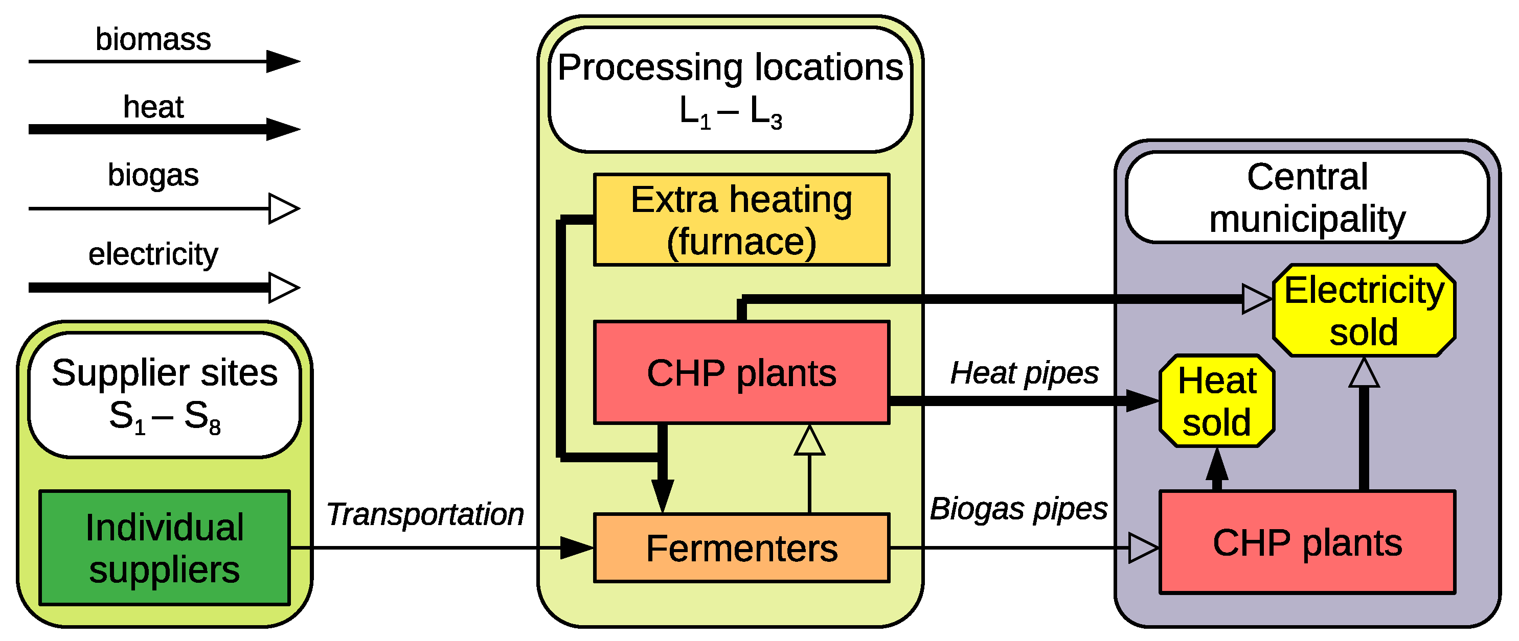
2.1. Problem Description

The goal of the original study was to produce heat and electricity from biomass in a small rural region around the town of Bad Zell (Austria). The supply chain is summarized in Figure 1.
Four types of biomass are available: animal manure, intercrops, grass, and corn silage. In fact, an objective of the original case study was to investigate the potential usage of intercrops.
There are dozens of individual agricultural suppliers for biomass. As a simplification, these are grouped into eight supplier sites. The available biomass is transported via trucks to one of the three possible processing locations. Biomass is transported as fresh matter, which means it is not dried first. This is acceptable due to the short distances.
Each location may host multiple fermenter units, which produce biogas (methane) from biomass, and multiple CHP plants. Biogas throughput is estimated based on the dry matter content of the fresh matter of each biomass type transported. Heat and biogas can be transferred via pipes to the central town, which can host additional CHP plants. Supporting infrastructure is also required: fermenters require heating, storage of biomass requires investing in a silo plate at each location, and electricity transfer requires a transformer. All purchased biomass and all produced biogas must be consumed inside the supply chain, no leftovers are allowed.
The optimization problem seeks to maximize profit from selling produced heat and electricity in the central town. It is assumed that all energy can be sold, there is no specific demand. The key decisions to be made are the locations, numbers, and sizes of the fermenter and CHP units, and they require supporting infrastructure to be invested into, and also determine material flows. A payoff period of 15 years was used in the original work.
Both fermenter and CHP units are available in different sizes: 80 kW, 160 kW, 250 kW, 500 kW. In the case of a CHP unit, the sizes denote electricity output. In the case of a fermenter unit, the size indicates that the fermenter can just supply a CHP unit of the same size with biogas if both work at full capacity. However, it is not required that the fermenter is actually connected to such a CHP plant, there can be any numbers and combinations of both, even with a partial utilization, as long as material balance for biogas is satisfied.
Fermenter inputs are a critical point in the model. The original case study assumed eight fixed input compositions for fermenters. These are shown in Table 1 along with total available amounts.
The exact method of selecting these fixed compositions was not available, although there was one explicitly mentioned restriction: manure usage must be at least 30%, due to a regulation. This is implicitly true if any of the fixed input compositions are used, but must be explicitly stated as a constraint when a flexible model is formulated.

2.2. Initial MILP Model

The main part of our work consists of an initial and a modified MILP model formulation and a P-Graph model formulation for the described problem. Symbols for sets, variables, and parameters are listed in Appendix A. Implementations and results are made available as Supplementary Materials.
The initial MILP model is now presented. The purpose of the initial MILP model was to reproduce results from the original case study, using fixed input fermenters. Constraints are listed below.
An important note: the key decision variables x k , m , l denoting fermenter utilization, and y k t o w n and y k , l denoting CHP plant utilization are not binary but integer variables, allowing multiple identical units.
Constraint (1) states that the fresh matter amounts b s , l , t o u t transported from suppliers to all locations l cannot exceed the total biomass availability B A V s , t at supplier s.
l L b s , l , t o u t B A V s , t s S , t T
The total of fresh matter amounts b s , l , t o u t transported to a location l is equal to the total of inputs b k , m , l , t i n of fermenters at that location, taking all sizes k and input compositions m into account. This is stated in Constraint (2).
s S b s , l , t o u t = k K , m M b k , m , l , t i n l L , t T
Constraint (3) calculates biogas production from input biomass types t, for all fermenters of size k, with input composition m, at location l. Two conditions must hold.
  • Ratio of inputs b k , m , l , t i n is determined by the input composition m. Constant B R m , t denotes the ratio for biomass type t in input composition m such that t T B R m , t = 1 .
  • The total amount g k , m , l of biogas is obtained as a sum for each input t. The factor T G t is used to convert fresh matter amounts to produce biogas amounts such that b k , m , l , t i n units of biomass type t yield a production of b k , m , l , t i n · T G t units of biogas.
g k , m , l · B R m , t · T G t t T B R m , t · T G t = b k , m , l , t i n · T G t k K , m M , l L , t T
Fermenter and CHP plant capacities are measured in full load working hours, of which F L H = 7800 is assumed a year. Fermenters of size k, composition m, at location l work for an equivalent of u k , m , l hours, although the exact distribution of load during the year is not considered in the model. For example, if a fermenter works at full, and another identical one at half capacity, then u k , m , l = 1.5 · F L H . In Constraint (4), coefficient W T B k converts the working capacity to biogas production depending only on equipment size.
u k , m , l F L H · W T B k = g k , m , l k K , m M , l L
Biogas material balance at each location captured by Constraint (5) means that all production g k , m , l is either transported to the town ( g l t r a n ) or consumed in place. Used working capacity of CHP plants of size k at location l is u k , l c h p .
k K , m M g k , m , l = g l t r a n + k K u k , l c h p F L H · W T B k l L
All biogas transported into the town are consumed by CHP plants. In Constraint (6), variable u k c h p , t o w n denotes working capacity of CHP plants of size k at the town.
l L g l t r a n = k K u k c h p , t o w n F L H · W T B k
Heat balance at each location l is established by Constraint (7). Heat is produced by CHP plants, calculated using the “working hours to heat” factor W T Q k , and extra heating q l e x t r a from a furnace. Heat is consumed by fermenters regarded by factor R E Q k , m or transported to the town, denoted by q l t r a n .
k K u k , l c h p · W T Q k + q l e x t r a = k K , m M u k , m , l F L H · R E Q k , m + q l t r a n l L
Heat pipes, if built, may carry heat from locations to the town. For each location l L to build a heat or biogas pipe from l to the town, P l P denotes the set of pipe sections that must be built. In short, our new formulation allows arbitrary pipe section requirements. In the original case study, there were 3 possible pipe sections: P 1 : from L 1 to town; P 2 : from L 2 to town; and P 3 : from L 3 to L 1 . Therefore, P L 1 = P 1 , P L 2 = P 2 , P L 3 = P 1 , P 3 .
Constraint (8) ensures that no more heat can be lost than being transported from any location l. Constraint (9) ensures that heat loss ( q p l o s s ) at a pipe section p is the sum of heat losses at that pipe section attributed to different locations ( q l , p l o s s ).
q l t r a n l L : p P l q l , p l o s s l L
q p l o s s = l P l q l , p l o s s p P
Heat loss q p l o s s at a pipe section is assumed to be proportional to pipe section length P S L p with a constant rate Q L . This is stated in Constraint (10). Binary variable z p q denotes whether the pipe section is built.
q p l o s s = z p q · P S L p · Q L p P
Constraint (11) states that the heat throughput to be sold is from direct production at the town, plus transported amounts, minus heat losses.
q s e l l = k K u k c h p , t o w n · W T Q k + l L q l t r a n l L , p P l q l , p l o s s
Electricity throughput e k s e l l to be sold is calculated separately for each CHP plant size k. Constraint (12) uses the constant factor W T E k to convert working capacity to electricity throughput.
e k s e l l = W T E k · u k c h p , t o w n + l L u k , l c h p k K
The following constraints state that if some investment is not made, and the represented infrastructure is not built (denoted by integer variables), then a corresponding activity cannot take place. If the investment is made, then there is still usually an upper bound. Due to implementation reasons, there are constants N i d for the maximum of identical equipment units at the same location or the town, and G M A X and Q M A X as an upper limit M for biogas and heat transportation.
For example, working capacity u k c h p , t o w n of CHP plants of size k at the town is, at maximum, the number of such plants ( y k t o w n ) times F L H . If a silo plate is built at a location ( z l s i l o ), then a maximum of N i d identical fermenters are allowed there ( x k , m , l ); otherwise, the maximum is 0.
u k c h p , t o w n y k t o w n · F L H k K
u k , l c h p y k , l · F L H k K , l L
u k , m , l x k , m , l · F L H k K
x k , m , l z l s i l o · N i d k K , m M , l L
y k t o w n z t r · N i d k K
y k , l z t r · N i d k K , l L
g l t r a n z l b g · G M A X l L
q l t r a n z l q · Q M A X l L
z p b g z l b g p P l
z p q z l q p P l
Annual income, calculated in Constraint (23), is from selling heat and electricity throughput. Due to regulations, the feed-in tariff P R k e for electricity depends on plant size k.
v i n = q s e l l · P R q + k K e k s e l l · P R k e
Investment costs are attributed to CHP plants, fermenters ( v i n v , f ), silo plates, the transformer, biogas pipes, and heat pipes. All investment costs are fixed, except that biogas and heat pipes also have costs proportional to length, and heat pipes do not have a fixed part. The investment costs are calculated in Constraint (24).
v o u t , i n v = k K , l L y k , l + k K y k t o w n · I N V k c h p + v i n v , f + l L z l s i l o · I N V s i l o + z t r · I N V t r + p P z p b g · I N V b g + p P z p b g · L E N p · I N V b g , p r o p + p P z p q · L E N p · I N V q , p r o p
Expenses are due to biomass purchase costs, biomass transportation with a fixed part and proportional to distance, silo operation, fermenter heating purchase, fermenter operation ( v o p , f ) and CHP plant operation, CHP plant electricity cost, and heat pipe electricity cost. These annual expenses are calculated in Constraint (25).
v o u t , o p = t T P R t · s , l b s , l , t o u t + s S , l L , t T b s , l , t o u t · T R t f i x + D I S T l , s · T R t p r o p + l L z l s i l o · O P s i l o + l L q l e x t r a · O P f , e x t r a + v o p , f + k K y k t o w n + k K , l L y k , l · O P k c h p + k K u k c h p , t o w n + k K , l L u k , l c h p · O P k c h p , e l + l L q l t r a n · O P p i p e , e l
Fermenter investment costs v i n v , f and operating costs v o p , f are calculated in Constraints (26) and (27) separately for better explaining model modifications.
v i n v , f = k K , m M , l L x k , m , l · I N V k , m f
v o p , f = k K , m M , l L x k , m , l · O P k f
A payback period of P B P = 15 years was used as in the original case study. The objective is the annual profit, which equals the revenues minus the annualized investment and operating costs.
max : v i n v o u t , i n v P B P v o u t , o p

2.3. Modified MILP Model with Flexible Inputs

The initial MILP model was modified to use fermenters with flexible inputs. The key change is that the fixed input compositions m M are not used, as each fermenter may have a variable input composition. To make it possible to have multiple such fermenters for the same size k and location l, a new identifier i is introduced instead of m. Constant N f is introduced as a practical maximum number of fermenters with flexible inputs of the same size and at a given location. For fermenters only, N f is a substitute of N i d for identical units. The identifier i runs over the set I = i : i Z , 1 i N f . The new binary variable denoting fermenter utilization (existence) is x k , i , l . Note that unlike the former x k , m , l , the new x k , i , l is binary, allowing a single fermenter. Therefore, there can be N f distinct fermenters with flexible inputs for any size k and location l.
As a consequence, heating demands and investment costs of fermenters are calculated based on the input amounts for each biomass type t instead of the fixed input composition m. Therefore, as shown later, parameters R E Q k , t and I N V k , t f are used instead of R E Q k , m and I N V k , m f .
Note that fermenters of different sizes k K are still distinguished in the new model as well. The reason is that costs for different sizes are rather unique, mainly due to economies of scale.
Constraint (2) is replaced by Constraint (29) as follows. Variable b k , i , l , t i n denotes the input of biomass type t into a single fermenter of size k, identifier i, at location l. The sum of inputs is the sum of delivered biomass amounts b s , l , t o u t .
s S b s , l , t o u t = k K , i I b k , i , l , t i n l L , t T
The new model allows a minimum ratio B R t m i n for all flexible fermenters, for any biomass type t. This is an example of the flexible input scheme allowing arbitrary linear constraints. In the original case study, the only such requirement was that there must be at least 30% manure. ( B R Manure m i n = 0.3 ). Constraint (30) formulates this requirement.
b k , i , l , t i n B R t m i n · t T b k , i , l , t i n k K , i I , l L , t T
The total biogas amount g k , i , l produced by a single fermenter is obtained as a sum for all input biomass types t. Constraint (31) is introduced, which replaces Constraint (3).
g k , i , l = t T b k , i , l , t i n · T G t k K , i I , l L
Fermenter working capacity u k , i , l is connected to biogas production by the factor W T B k . Constraint (32) is introduced, which is similar to the original Constraint (4), and replaces it.
u k , i , l F L H · W T B k = g k , i , l k K , i I , l L
Constraint (5) is replaced by Constraint (33) to express biogas balance at locations. The produced biogas is either transported to the town ( g l t r a n ) or consumed by local CHP plants.
k K , i I g k , i , l = g l t r a n + k K u k , l c h p F L H · W T B k l L
A similar replacement is done from Constraint (7) expressing heat balance at locations. A significant change is that the fermenter heating requirement is not based on working hours and parameter R E Q k , m for each input composition m. Heating requirement is instead assumed to be proportional to input amounts, expressed by the new parameter R E Q k , t for each biomass type t. The new Constraint (34) states that the amount generated by CHP plants plus the purchased extra heating is either consumed by fermenters or transported to the town.
k K u k , l c h p · W T Q k + q l e x t r a = k K , i I , t T b k , i , l , t i n · R E Q k , t + q l t r a n l L
The logical Constraint (16) expressing silo plate usage is also replaced by Constraint (35). The silo plate is needed if there is a fermenter at the location.
x k , i , l z l s i l o k K , i I , l L
Similarly, Constraint (27) is replaced by Constraint (36). The annual operating cost of any fermenter of size k is O P k f as in the initial model.
v o p , f = k K , i I , l L x k , i , l · O P k f
Fermenter investment costs are more difficult to formulate. A linear estimation is made based on the amounts b k , i , l , t i n , as for the heating requirement in Constraint (34). A new parameter I N V k , t f is introduced for the investment cost per unit amount of biomass type t consumed. The following is a possible estimation of the investment cost (not included as a constraint).
v i n v , f = k K , i I , l L , t T b k , i , l , t i n · I N V k , t f
The issue with Equation (37) is that the investment cost should not scale down if a fermenter is used below full capacity and consumes less. For this reason, the slack biogas amount g k , i , l s l a c k is also calculated for each fermenter, by a new Constraint (38). This slack is the amount that is actually not produced but would be if the fermenter was working at full capacity. Variable x k , i , l denotes whether the fermenter is built.
x k , i , l · W T B k = g k , i , l s l a c k + g k , i , l k K , i I , l L
Therefore, g k , i , l s l a c k + g k , i , l depends only on k, not on the inputs. Since the biogas production from t is b k , i , l , t i n · T G t , the value I N V k , t f , b g = I N V k , t f · T G t 1 expresses investment cost per unit biogas production.
The idea is to calculate the investment cost based on the slack as if it was the actual consumption of biomass type t with maximal I N V k , t f , b g . With this choice, the calculated investment cost is an upper bound of the actual one, being strict if the fermenter is used at full capacity, or if the fermenter only uses inputs t for which I N V k , t f , b g is maximal. Constraint (39) performs the aforementioned calculation of the fermenter investment costs.
v i n v , f = k K , i I , l L g k , i , l s l a c k · max t T I N V k , t f , b g + t T b k , i , l , t i n · I N V k , t f

2.4. P-Graph Model, Flexible Inputs
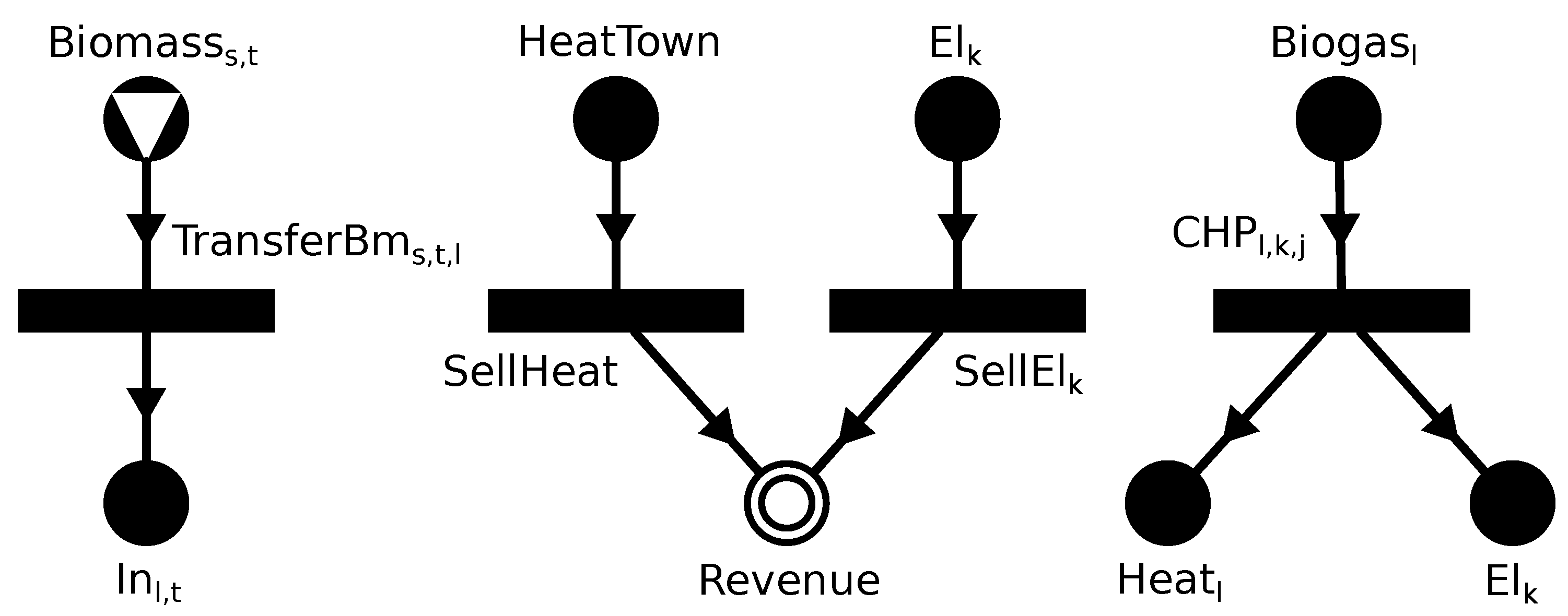
The maximal structure of the P-Graph model is too large to be depicted as a whole. Instead, operating unit nodes are detailed here. Node labels are listed in the nomenclature.
The raw material nodes are Biomass ̲ s , t for available biomass types t at suppliers s, and HeatPlus ̲ for extra heating. The single product node is Revenue ̲ . Subtracting costs of the network from the Revenue ̲ amount gives the objective.
Some operations, like material transfers or conversions, listed below, can be modeled by an operating unit with a single input material.
  • Operating units TransferBm ̲ s , t , l for biomass transfer are introduced for each supplier s, biomass type t, and location l. The single input material node is Biomass ̲ s , t , and the output is In ̲ l , t , which represents the input for fermenters.
  • Operating units BuyHeat ̲ l denote purchase of HeatPlus ̲ into the available heat Heat ̲ l for each location l.
  • Operating units TransferBg ̲ l denote transportation of available biogas Biogas ̲ l at each location l to the town, denoted by the BiogasTown ̲ node.
  • Operating units SellHeat ̲ and SellEl ̲ k for all sizes k denote selling energy. Their single inputs are HeatTown ̲ and El ̲ k , and the output is Revenue ̲ in all cases.
  • The CHP plant at location l, with size k, and identifier j is denoted by operating unit node CHP ̲ l , k , j . Since N i d identical plants are allowed, 1 j N i d . The single input is the available biogas Biogas ̲ l , and the two outputs are available heat Heat ̲ l and electricity El ̲ k .
  • The CHP plant at the town, with size k and identifier j is modeled similarly, by operating unit node CHPTown ̲ k , j . The single input is BiogasTown ̲ , and the two outputs are available heat HeatTown ̲ and electricity El ̲ k .
Figure 2 shows three of the aforementioned operations. In the final P-Graph model, individual nodes are introduced for each index set.
If an operating unit requires another operating unit to be present, it can be modeled by a logical constraint. The required operating unit produces a dummy capacity material, which is consumed by the depending operating unit. The exact amounts of the dummy capacity material are not important.
Logical constraints of this kind are applied to operating unit nodes representing investment into some equipment. Instances are listed below. Examples are shown in Figure 3.
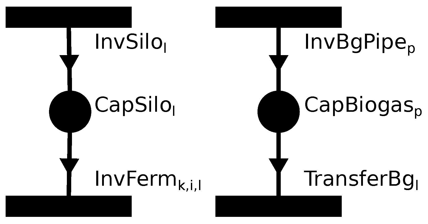
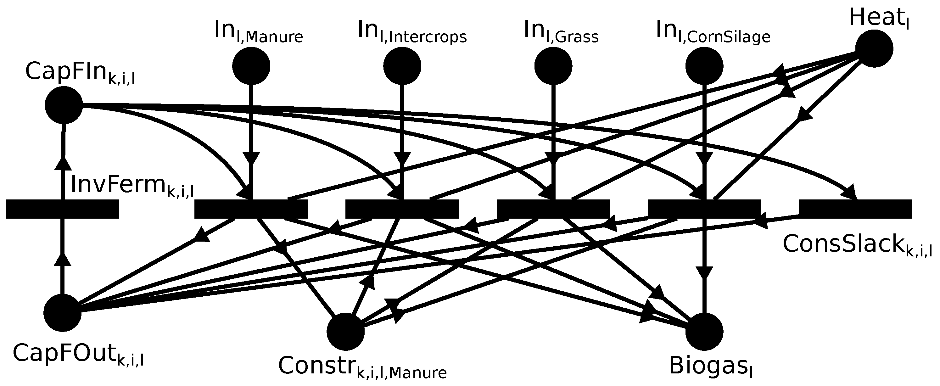
  • Investment into the fermenter of size k, identifier i, location l, is denoted by operating unit InvFerm ̲ k , i , l . It requires the silo plate, denoted by operating unit InvSilo ̲ l and dummy capacity material CapSilo ̲ l .
  • CHP plant operation for any size k and identifier j at the town ( CHP ̲ l , k , j ) or a location l ( CHPTown ̲ k , j ) requires the transformer, denoted by operating unit InvTr ̲ and capacity CapTr ̲ .
  • Biogas transfer from any location l denoted by operating unit TransferBg ̲ l across a pipe section p P l requires building that pipe section, denoted by operating unit InvBgPipe ̲ p and capacity CapBiogas ̲ p .
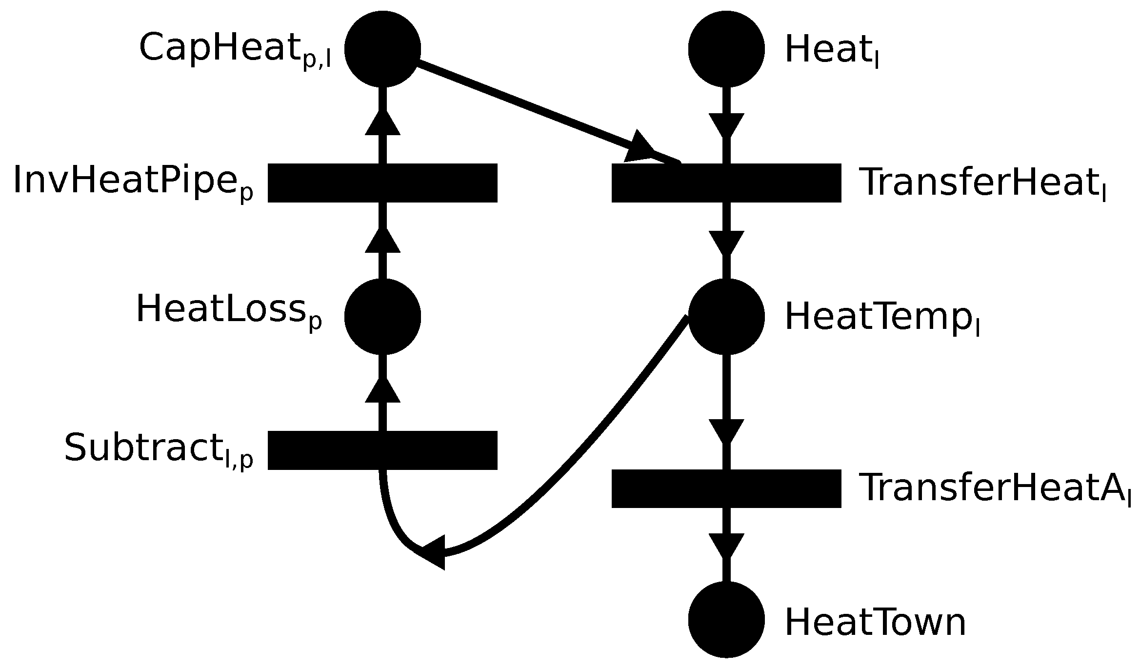
  • Heat transfer has the same rules as biogas transfer, but due to different heat loss and cost calculations, the implementation is different. TransferHeat ̲ l is the operating unit for heat transfer, and InvHeatPipe ̲ p is the operating unit for heat pipe investment, but there are distinct capacities CapHeat ̲ p , l for each l, p P l .
The model of the fermenters with flexible inputs is the most complex. It is shown in Figure 4, and is now detailed. The basic flexible input technique from [5] is involved, and is further extended.
The size k, identifier i (with 1 i N f ), and location l together identify a single fermenter unit. For all four biomass types t, namely: manure, intercrops, grass, and corn silage, operating unit node ConsFerm ̲ k , i , l , t represent consumption of input materials In ̲ l , t . Nodes ConsFerm ̲ k , i , l , t play the key role, in the following ways.
  • Input node Heat ̲ l represents the required fermenter heating, which depends on the amounts of each t with its specific flow rate.
  • The 30% minimum ratio of manure is ensured by a single logical material node Constr ̲ k , i , l , M a n u r e , produced by ConsFerm ̲ k , i , l , M a n u r e (second operating unit in Figure 4) with flow rate 7, and consumed by ConsFerm ̲ k , i , l , t for all other biomass types t with flow rate 3.
  • InvFerm ̲ k , i , l represents the investment into the fermenter, producing its full capacity CapFIn ̲ k , i , l , which is then consumed by each ConsFerm ̲ k , i , l , t , and also ConsSlack ̲ k , i , l . This structure is mirrored: CapFOut ̲ k , i , l is produced, which is an input to InvFerm ̲ k , i , l . This ensures that ConsSlack ̲ k , i , l consumes all the remaining capacity. Therefore, the investment cost can be calculated based on the amounts processed by ConsFerm ̲ k , i , l , t and ConsSlack ̲ k , i , l .
  • Biogas ̲ l is the output of all production except for the slack, with appropriate flow rates for each biomass type t.
The last remaining part is the calculation of heat loss, which is a fixed term in this model for each pipe section p P , but the required pipe sections p P l for a location l can be arbitrary. The model is shown in Figure 5. Nodes with indices l, p, or pair of l and p are introduced for each index l L , p P or pair of l L and p P l , respectively.
Heat transfer from Heat ̲ l does not immediately go into HeatTown ̲ but into a temporary material HeatTemp ̲ l of which only a part is forwarded to HeatTown ̲ . Some amount is subtracted by operating unit Subtract ̲ l , p into HeatLoss ̲ p representing heat loss amounts. This happens for each p P l . Finally, if a sufficient amount of HeatLoss ̲ p is present, operating unit InvHeatPipe ̲ p produces all dummy capacity materials CapHeat ̲ p , l for which p P l . Note that InvHeatPipe ̲ p also models investment into the heat pipe section p.
This part of the formulation is rather cumbersome. A future goal of our research is to find a simple technique for achieving a similar modeling goal.

3. Results

Model data were obtained from the original case study [6] and the corresponding project report [7]. Some of these data were not explicitly stated in these sources but were determined by inspecting the reported results. These sources also provide insight into using intercrops for biogas production.

3.1. Parameter Estimation

The modified model needs two new parameters not available from the original data: R E Q k , t and I N V k , t f , expressing fermenter heating requirement and investment cost.
In an effort to provide useful estimations for these parameters, multiple linear regression was performed based on the original R E Q k , m and I N V k , m f for the M = 8 known input compositions. Investment and heating costs are expressed as a linear function of input biomass amounts for each of the four biomass types t, without a constant term.
There were K = 4 possible sizes: 80 kW, 160 kW, 250 kW, 500 kW. In the case of fermenters, these power values are proportional to biogas production and, consequently, biomass consumption in both models. Since the heating requirement seems to almost perfectly scale linearly with plant size, a single instance of multiple linear regression was performed for all sizes k, and the obtained value was used for all sizes k. Therefore, R E Q k , t is a constant for all sizes k, only depending on biomass type t. Investment costs are significantly affected by the economies of scale, so the regression was made for each size k individually. Consequently, values of I N V k , t f depend on both k and t. The obtained values are shown in Table 2. For example, a fully utilized 160 kW fermenter has a heating requirement of 160 times 0.0412 MW and an investment cost of 55.95 EUR per each m3 of manure consumed.
Since the conversion factor T G t is significantly lower for manure than for any other t, the parameter I N V k , t f is maximal for manure, for all k. Therefore, manure is used for calculating investment costs for slack amounts in the modified model.
To verify the results, the values of R E Q k , t and I N V k , t f can be used to recalculate R E Q k , m and I N V k , m f in the initial MILP model for each fixed input composition m. The difference from the original values was between −7.8% and 6.5%, indicating that the estimation functions are acceptable. More importantly, this recalculation allows us to solve the initial and the modified MILP models on exactly the same data. All other parameter values not mentioned here can be found in the Supplementary Materials.

3.2. MILP Model Results

Three MILP model solutions were made.
  • Initial model (fixed inputs) with original data.
  • Initial model (fixed inputs) with recalculated R E Q k , m and I N V k , m f .
  • Modified model (flexible inputs) with estimated R E Q k , t and I N V k , t f .
All MILP models were written in GNU MathProg language, and GLPSOL was used as the MILP solver. The case study features L = 3 locations. N i d = 3 and N f = 2 were used in the models, which means, at most, three identical buildings, but two flexible fermenters at the same locations. This latter choice turned out to be sufficient.
The solution of the initial model with fixed inputs, detailed later, was compared to the results reported in the original case study. The annual profit of 234,544 EUR was obtained, while the original study reported 196,350 EUR. The difference is due to the different modeling of transportation costs of biomass, as it was ambiguously described and we could not reproduce it perfectly. The two fermenters are built at L 3 in the original study, but at L 1 in the reproduced MILP model, but they have the same inputs. Also, the study reported a solution using all CHP plants in the town, not at L 1 , where more fermenter heating was purchased. All other decisions and cost terms, for example, fermenter inputs, plant sizes, pipe and infrastructure utilization, and their costs in the model coincide. The initial model and its solution serve as a basis for comparison.
The solution of the initial model with the new, estimated data was compared to the solution with the original data to see how accurate the parameter estimations were. The two solutions have slightly different values for fermenter heating and investment costs (shown in Table 3). Otherwise, the exact same decisions were made, including fermenter and CHP plant selection and biomass transportation. This indicates that the estimations are accurate.
The second solution uses the initial MILP model with fixed inputs, and the third solution uses the modified MILP model with flexible inputs, while the model data are exactly the same, including the parameter estimations. This makes a fair comparison of the models possible.
The solutions are significantly different this time, as shown in Table 4. The larger search space of the modified model with flexible inputs results in a better utilization of resources. More biomass is used. The 500 kW fermenter with flexible inputs is more economical than the two 250 kW fermenters due to economies of scale. Despite the 80 kW extra throughput, the total investment costs are not much higher. On the other hand, the two 250 kW CHP plants were chosen instead of one 500 kW CHP plant, since the feed-in tariff for the larger plant is lower. Overall, the annual profit is 31.62% better. The model for flexible inputs is also smaller and faster to solve. The results suggest that it is better to use flexible inputs for optimization and designing fermenters based on the results, if such a workflow is possible, than using some fixed fermenter designs and optimizations assuming them. Note that a requirement for a flexible model is an accurate estimation of parameters depending on input composition. This particularly applies to heat requirements and investment costs in our case study. Inaccurate calculations of these may cause a reported solution to be inefficient or infeasible in reality. Since biomass sources can fluctuate, it is also advisable to rely on technologies that can handle input fluctuations by design.

3.3. P-Graph Results

The P-Graph problem formulation consists of not only the P-Graph, but also the data of the nodes and arcs, like flow rates, minimum and maximum usages, purchase costs, revenues, investment, and operating costs. These were determined according to the case study data, including the parameter estimations.
The formulation was generated using a Python script. This was used as a tool to programmatically construct the graph in the format excepted by the P-Graph solver. The generated P-Graph consists of 147 material nodes, 319 operating unit nodes, and 1144 arcs, with N f = 2 fermenters and N i d = 3 CHP plants of the same kind allowed.
The P-Graph solver used the ABB algorithm. The solver successfully finished in 413.45   s on a Dell Latitude E5470 laptop, with Intel i7.6600 CPU, and 16 GB RAM. The solver version was v2.0.3, running on Windows 10.
The P-Graph model formulation was proven to be a working alternative to MILP models. The exact same solution was obtained for the modified MILP model, indicating that the two approaches are equivalent. The higher computational time can be attributed to several differences. First, the ABB algorithm for P-Graphs has the advantage of naturally producing not only the best but the set of solution structures ordered by objective. These alternative solutions were not investigated in this work. The P-Graph model has some redundancy, by introducing fermenters and CHP plants of the same kind as duplicate components in the graph. This could possibly be mitigated if the P-Graph implementation allowed integer variables for operating units instead of a single binary variable which can only represent a single unit.
The P-Graph solver has an option to export an MILP model equivalent to the P-Graph model. This was done. The exported MILP model is different from the MILP models presented. In fact, it itself inherits the redundancy of the P-Graph formulation. This results in GLPSOL being unable to prove optimality in 1000 s, but another MILP solver, CBC, was able to conclude that the optimal solution in 19.99   s . Therefore, a strong MILP solver may outperform the ABB algorithm, indicating that redundancy may be handled better.
Nevertheless, the P-Graph framework was suitable for modeling and solving the case study as the modified MILP model with flexible inputs, although solution speed could be improved.

4. Conclusions

In this work, MILP and P-Graph models for a case study involving biomass-based energy production in a small rural area were presented. The main improvement compared to the originally published results was the usage of flexible inputs for modeling fermenter units. The original study involved several predetermined, fixed input compositions of fermenters to choose from. In contrast, the flexible models presented here allow the input compositions to be model variables, resulting in a wider search space and better solutions.
The original study was reproduced first as an MILP model with the original fixed inputs. Then, estimations were made for the fermenter heating requirement and investment cost parameters, which were necessary for any model with flexible inputs. Then, a modified MILP model allowing flexible inputs and a P-Graph model were developed.
The modified MILP model using flexible inputs outperformed the MILP model using fixed inputs. The profit was 31% higher, with better biomass utilization and with a model that is faster to solve. This shows that it is better to optimize for the input compositions and then design equipment based on the results, if possible, than assuming a set of fixed input compositions and optimizing based on them. The P-Graph model using the recently published technique of flexible inputs was able to provide the same optimal solution as the modified MILP model. However, the solver runtime is worse, possibly due to the ABB algorithm not handling redundancy well. Another reason is that ABB reports a set of solutions instead of a single optimal solution. A future direction of research could be the improvement of both the algorithmic framework for P-Graphs and the modeling techniques as well. For example, a more efficient technique for modeling heat pipes could likely be found.

Supplementary Materials

The following supporting information can be downloaded at: https://www.mdpi.com/article/10.3390/en17030687/s1. Data used in the case study, the source codes of all MILP and P-Graph models, and obtained results are attached as supplementary materials.

Author Contributions

Methodology, A.É.; supervision, I.H.; validation, I.H. and H.C.; writing—original draft preparation, A.É.; writing—review and editing I.H. and H.C. All authors have read and agreed to the published version of the manuscript.

Funding

This work has been implemented by the TKP2021-NVA-10 project with the support provided by the Ministry of Culture and Innovation of Hungary from the National Research, Development, and Innovation Fund, financed under the 2021 Thematic Excellence Programme funding scheme.

Data Availability Statement

Data are contained within the article and supplementary material.

Conflicts of Interest

The authors declare no conflict of interest. The funders had no role in the design of the study; in the collection, analyses, or interpretation of data; in the writing of the manuscript; or in the decision to publish the results.

Appendix A. Nomenclature

Appendix A.1. Sets

l L Set of (processing) locations.
k K Set of plant sizes.
m M Set of fixed fermenter input compositions (or mixtures).
p P Set of possible pipe sections between locations and/or the town.
p P l Set of required pipe sections for location l L . P l P
s S Set of suppliers.
t T Set of raw material (biomass) types.
i I Set of identifiers for distinct fermenters with flexible inputs. I = i : i Z , 1 i N f

Appendix A.2. Integer Variables

x k , i , l The fermenter with flexible inputs of size k, identifier i, at location l, is built.
x k , m , l Number of fermenter units of size k with input composition m built at location l.
y k t o w n Number of CHP plants of size k built in the town.
y k , l Number of CHP plants of size k built at location l.

Appendix A.3. Binary Variables

z l b g Produced biogas is transported from location l.
z p b g Biogas pipe is built between the endpoints of pipe section p.
z l q Produced heat is transported from location l.
z p q Heat pipe is built between the endpoints of pipe section p.
z l s i l o A silo plate is built at location l.
z t r A transformer is built.

Appendix A.4. Nonnegative Real Variables

b s , l , t o u t Amount of biomass type t (fresh matter) transported from supplier s to location l.
b k , i , l , t i n Amount of biomass type t (fresh matter) fed into the fermenter with flexible inputs of size k, identifier i, at location l.
b k , m , l , t i n Amount of biomass type t (fresh matter) fed into fermenters of size k with input composition m at location l.
e k s e l l Total electricity throughput to be sold, from CHP plants of size k.
g k , i , l Amount of biogas produced by the fermenter with flexible inputs of size k, identifier i, at location l.
g k , i , l s l a c k Slack amount of biogas corresponding to the fermenter with flexible inputs of size k, identifier i, at location l.
g k , m , l Amount of biogas produced by fermenters of size k with input composition m at location l.
g l t r a n Amount of biogas transported from location l to the town.
u k c h p , t o w n Working capacity spent by CHP plants of size k at the town.
u k , l c h p Working capacity spent by CHP plants of size k at location l.
u k , i , l Working capacity spent by the fermenter with flexible inputs of size k, identifier i, at location l.
u k , m , l Working capacity spent by fermenters of size k with input composition m at location l.
q l e x t r a Heating purchased for fermenters at location l.
q l t r a n Heat transported from location l to the town.
q p l o s s Heat loss during transportation at pipe section p.
q l , p l o s s Heat loss during transportation from location l to the town, attributed to pipe section p P l .
q s e l l Total heat sold.
v i n Total income per year.
v i n v , f Fermenter investment costs, annualized.
v o p , f Fermenter operating costs per year.
v o u t , i n v Total investment costs, annualized.
v o u t , o p Total operating costs, annualized.

Appendix A.5. Parameters

B A V s , t Available amount of biomass type t at supplier s.
B R m , t Ratio of biomass type t in the fermenter input composition m.
B R t m i n Minimum input ratio for biomass type t in each fermenter.
D I S T l , s Distance of location l from supplier s.
F L H Full load working hours during a year.
G M A X M value, constant upper limit for biogas transported.
I N V b g Fixed investment cost of a biogas pipe.
I N V b g , p r o p Investment cost of a biogas pipe proportional to length.
I N V q , p r o p Investment cost of a heat pipe proportional to length.
I N V k c h p Investment cost of a CHP plant of size k.
I N V k , m f Investment cost of a fermenter of size k with fixed input composition m.
I N V s i l o Investment cost of a silo plate at a location.
I N V t r Investment cost of the transformer.
I N V k , t f Fermenter investment cost per unit amount of biomass type t consumed, at full capacity, assuming a fermenter with flexible inputs of size k.
I N V k , t f , b g Fermenter investment cost per unit amount of biogas produced from biomass type t consumed, at full capacity, assuming a fermenter with flexible inputs of size k.
N f Number of identical fermenters with flexible inputs allowed.
N i d Maximum number of identical units at a location or the town.
O P k c h p Annual operating cost of a CHP plant of size k.
O P k c h p , e l Electricity cost of a CHP plant of size k per working capacity.
O P f , e x t r a Unit cost of fermenter heating.
O P k f Annual operating cost of a fermenter of size k.
O P p i p e , e l Electricity cost per unit of heat transported.
O P s i l o Annual operating cost of a silo plate.
P B P Payback period assumed, in years.
P S L p Length of pipe section p.
P R t Purchase price of biomass type t.
P R q Sell price of heat produced.
P R k e Sell price of electricity produced at a CHP plant of size k.
Q M A X M value, constant upper bound for heat transported.
Q L Constant rate of heat loss.
R E Q k , m Heating required by a fermenter of size k with composition m.
R E Q k , t Fermenter heating required per unit amount of biomass type t consumed, assuming a fermenter with flexible inputs of size k.
T G t Conversion factor from fresh matter amount of biomass type t to biogas amount.
T R t f i x Fixed transportation cost of biomass type t.
T R t p r o p Transportation cost of biomass type t, proportional to distance.
W B T k Conversion factor from working capacity of fermenters of size k to biogas amount produced.
W T Q k Conversion factor from working capacity of CHP plants of size k to heat produced.
W T E k Conversion factor from working capacity of CHP plants of size k to electricity produced.

Appendix A.6. P-Graph Material Nodes

All material nodes are intermediate material nodes unless otherwise noted.
Biomass ̲ s , t Raw material node. Available biomass type t at supplier s.
Biogas ̲ l Biogas available at location l.
BiogasTown ̲ Biogas available at the town.
CapBiogas ̲ p Dummy capacity for biogas pipe section p.
CapFIn ̲ k , i , l Capacity on the input side, for the fermenter with flexible inputs, of size k, identifier i, location l.
CapFOut ̲ k , i , l Capacity on the output side, for the fermenter with flexible inputs, of size k, identifier i, location l.
CapHeat ̲ p , l Dummy capacity for the heat pipe from l, to ensure heat loss at pipe section p P l .
CapSilo ̲ l Dummy capacity for the silo plate at location l.
CapTr ̲ Dummy capacity for the transformer.
Constr ̲ k , i , l , t Material for constraint on the minimum ratio of input biomass type t, for the fermenter with flexible inputs, of size k, identifier i, location l.
El ̲ k Electricity produced by CHP plants of size k.
HeatPlus ̲ Raw material node. Extra heating purchased for fermenters.
Heat ̲ l Heating available at location l.
HeatTown ̲ Heating available at the town.
HeatTemp ̲ l Heating transferred from location l.
HeatLoss ̲ p Heat loss at pipe section p.
In ̲ l , t Input biomass type t at location l.
Revenue ̲ Product node. Revenue from selling heating and electricity.

Appendix A.7. P-Graph Operating Unit Nodes

BuyHeat ̲ l Purchase of extra heat at location l.
CHP ̲ l , k , j CHP plant at location l, of size k, identifier j.
CHPTown ̲ k , j CHP plant at the town, of size k, identifier j.
ConsFerm ̲ k , i , l , t Fermenter with flexible inputs, of size k, identifier i, location l, consuming biomass type t.
ConsSlack ̲ k , i , l Fermenter with flexible inputs, of size k, identifier i, location l, consuming remaining free (slack) capacity.
InvSilo ̲ l Invesment into the silo plate at location l.
InvFerm ̲ k , i , l Invesment into the fermenter with flexible inputs, of size k, identifier i, location l.
InvSilo ̲ l Invesment into the silo plate at location l.
InvBgPipe ̲ p Invesment into the biogas pipe section p.
InvHeatPipe ̲ p Invesment into the heat pipe section p.
InvTr ̲ Invesment into the transformer.
TransferBm ̲ s , t , l Transfer of biomass type t from supplier s to location l.
TransferBg ̲ l Transfer of biogas from location l to the town.
TransferHeat ̲ l Transfer of heating from location l to the town.
TransferHeatA ̲ l Arrival of heating (after losses) from location l to the town.
SellEl ̲ k Selling electricity from CHP plants of size k.
SellHeat ̲ Selling heating.
Subtract ̲ l , p Logical operating unit for subtracting heat loss from location l across pipe section p.

References

  1. Ó Céileachair, D.; O’Shea, R.; Murphy, J.D.; Wall, D.M. The effect of seasonal biomass availability and energy demand on the operation of an on-farm biomethane plant. J. Clean. Prod. 2022, 368, 133129. [Google Scholar] [CrossRef]
  2. Searcy, E.; Flynn, P.; Ghafoori, E.; Kumar, A. The relative cost of biomass energy transport. Appl. Biochem. Biotechnol. 2007, 137, 639–652. [Google Scholar] [CrossRef] [PubMed]
  3. Sun, O.; Fan, N. A Review on Optimization Methods for Biomass Supply Chain: Models and Algorithms, Sustainable Issues, and Challenges and Opportunities. Process Integr. Optim. Sustain. 2020, 4, 203–226. [Google Scholar] [CrossRef]
  4. Friedler, F.; Ákos, O.; Losada, J.P. P-Graphs for Process Systems Engineering, 1st ed.; Springer: Cham, Switzerland, 2022. [Google Scholar] [CrossRef]
  5. Éles, A.; Heckl, I.; Cabezas, H. Modeling technique in the P-Graph framework for operating units with flexible input ratios. Cent. Eur. J. Oper. Res. 2021, 29, 463–489. [Google Scholar] [CrossRef]
  6. Niemetz, N.; Kettl, K.H.; Szerencsits, M.; Narodoslawsky, M. Economic and ecological potential assessment for biogas production based on intercrops. In Biogas, 1st ed.; InTech: Rijeka, Croatia, 2012; pp. 173–190. [Google Scholar] [CrossRef]
  7. Szerencsits, M. Ökocluster—Klima und Wasserschutz Durch Synergetische Biomassenutzung—Biogas aus Zwischenfrüchten, Rest- und Abfallstoffen ohne Verschärfung der Flächenkonkurrenz; Technical Report; Klima- und Energiefonds: Wien, Austria, 2011. [Google Scholar]
  8. Éles, A.; Heckl, I.; Cabezas, H. Modeling Renewable Energy Systems in Rural Areas with Flexible Operating Units. Chem. Eng. Trans. 2021, 88, 643–648. [Google Scholar] [CrossRef]
  9. McKendry, P. Energy production from biomass (part 1): Overview of biomass. Bioresour. Technol. 2002, 83, 37–46. [Google Scholar] [CrossRef]
  10. McKendry, P. Energy production from biomass (part 2): Conversion technologies. Bioresour. Technol. 2002, 83, 47–54. [Google Scholar] [CrossRef]
  11. Bajwa, D.S.; Peterson, T.; Sharma, N.; Shojaeiarani, J.; Bajwa, S.G. A review of densified solid biomass for energy production. Renew. Sustain. Energy Rev. 2018, 96, 296–305. [Google Scholar] [CrossRef]
  12. Ba, B.H.; Prins, C.; Prodhon, C. Models for optimization and performance evaluation of biomass supply chains: An Operations Research perspective. Renew. Energy 2016, 87, 977–989. [Google Scholar] [CrossRef]
  13. Rentizelas, A.A.; Tatsiopoulos, I.P.; Tolis, A. An optimization model for multi-biomass tri-generation energy supply. Biomass Bioenergy 2009, 33, 223–233. [Google Scholar] [CrossRef]
  14. Kim, J.; Realff, M.J.; Lee, J.H.; Whittaker, C.; Furtner, L. Design of biomass processing network for biofuel production using an MILP model. Biomass Bioenergy 2011, 35, 853–871. [Google Scholar] [CrossRef]
  15. Kalaitzidou, M.A.; Georgiadis, M.C.; Kopanos, G.M. A General Representation for the Modeling of Energy Supply Chains. Comput. Aided Chem. Eng. 2016, 38, 781–786. [Google Scholar] [CrossRef]
  16. Sharma, B.; Ingalls, R.G.; Jones, C.L.; Khanchi, A. Biomass supply chain design and analysis: Basis, overview, modeling, challenges, and future. Renew. Sustain. Energy Rev. 2013, 24, 608–627. [Google Scholar] [CrossRef]
  17. Martín, M.; Grossmann, I.E. Energy optimization of hydrogen production from lignocellulosic biomass. Comput. Chem. Eng. 2011, 35, 1798–1806. [Google Scholar] [CrossRef]
  18. Cao, Y.; Dhahad, H.A.; Hussen, H.M.; Anqi, A.E.; Farouk, N.; Issakhov, A. Development and tri-objective optimization of a novel biomass to power and hydrogen plant: A comparison of fueling with biomass gasification or biomass digestion. Energy 2022, 238, 122010. [Google Scholar] [CrossRef]
  19. Tilahun, F.B.; Bhandari, R.; Mamo, M. Design optimization of a hybrid solar-biomass plant to sustainably supply energy to industry: Methodology and case study. Energy 2021, 220, 119736. [Google Scholar] [CrossRef]
  20. Nemet, A.; Klemeš, J.J.; Duić, N.; Yan, J. Improving sustainability development in energy planning and optimisation. Appl. Energy 2016, 184, 1241–1245. [Google Scholar] [CrossRef]
  21. Friedler, F.; Tarjan, K.; Huang, Y.W.; Fan, L.T. Graph-Theoretic Approach to Process Synthesis: Axioms and Theorems. Chem. Eng. Sci. 1992, 47, 1973–1988. [Google Scholar] [CrossRef]
  22. Friedler, F.; Tarjan, K.; Huang, Y.W.; Fan, L.T. Graph-Theoretic Approach to Process Synthesis: Polynomial Algorithm for the Maximal Structure Generation. Comput. Chem. Eng. 1993, 17, 929–942. [Google Scholar] [CrossRef]
  23. Friedler, F.; Varga, J.B.; Fan, L.T. Decision-Mapping: A tool for consistent and complete decisions in process synthesis. Chem. Eng. Sci. 1995, 50, 1755–1768. [Google Scholar] [CrossRef]
  24. Friedler, F.; Varga, B.J.; Fehér, E.; Fan, L.T. Combinatorially Accelerated Branch-and-Bound Method for Solving the MIP Model of Process Network Synthesis. In State of the Art in Global Optimization; Floudas, C.A., Pardalos, P.M., Eds.; Kluwer Academic Publishers: Dordrecht, The Netherlands, 1996; pp. 609–626. [Google Scholar]
  25. P-Graph Official Website. Available online: http://www.p-graph.org (accessed on 27 July 2023).
  26. Lam, H.L. Extended P-graph applications in supply chain and Process Network Synthesis. Curr. Opin. Chem. Eng. 2013, 4, 475–486. [Google Scholar] [CrossRef]
  27. Lam, H.L.; Chong, K.H.; Tan, T.K.; Ponniah, G.D.; Tin, Y.T.; How, B.S. Debottlenecking of the Integrated Biomass Network with Sustainability Index. Chem. Eng. Trans. 2017, 61, 1615–1620. [Google Scholar] [CrossRef]
  28. Atkins, M.J.; Walmsley, T.G.; Ong, B.H.Y.; Walmsley, M.R.W.; Neale, J.R. Application of P-graph techniques for efficient use of wood processing residues in biorefineries. Chem. Eng. Trans. 2016, 52, 499–504. [Google Scholar] [CrossRef]
  29. How, B.S.; Hong, B.H.; Lam, H.L.; Friedler, F. Synthesis of multiple biomass corridor via decomposition approach: A P-graph application. J. Clean. Prod. 2016, 130, 45–57. [Google Scholar] [CrossRef]
  30. Safder, U.; Lim, J.Y.; How, B.S.; Ifaei, P.; Heo, S.; Yoo, C. Optimal configuration and economic analysis of PRO-retrofitted industrial networks for sustainable energy production and material recovery considering uncertainties: Bioethanol and sugar mill case study. Renew. Energy 2022, 182, 797–816. [Google Scholar] [CrossRef]
  31. Lam, H.L.; Varbanov, P.S.; Klemeš, J.J. Optimisation of regional energy supply chains utilising renewables: P-graph approach. Comput. Chem. Eng. 2010, 34, 782–792. [Google Scholar] [CrossRef]
  32. Heckl, I.; Friedler, F.; Fan, L.T. Solution of separation-network synthesis problems by the P-graph methodology. Comput. Chem. Eng. 2010, 34, 700–706. [Google Scholar] [CrossRef]
  33. Bartos, A.; Bertók, B. Production line balancing by P-graphs. Optim. Eng. 2020, 21, 567–584. [Google Scholar] [CrossRef]
  34. Aviso, K.B.; Chiu, A.S.F.; Demeterio, F.P.A.; Lucas, R.I.G.; Tseng, M.L.; Tan, R.R. Optimal human resource planning with P-graph for universities undergoing transition. J. Clean. Prod. 2019, 224, 811–822. [Google Scholar] [CrossRef]
  35. Bertók, B.; Bartos, A. Algorithmic Process Synthesis and Optimisation for Multiple Time Periods Including Waste Treatment: Latest Developments in P-graph Studio Software. Chem. Eng. Trans. 2018, 70, 97–102. [Google Scholar] [CrossRef]
  36. Kalauz, K.; Süle, Z.; Bertók, B.; Friedler, F.; Fan, L.T. Extending Process-Network Synthesis Algorithms with Time Bounds for Supply Network Design. Chem. Eng. Trans. 2012, 29, 259–264. [Google Scholar] [CrossRef]
  37. Frits, M.; Bertók, B. Process Scheduling by Synthesizing Time Constrained Process-Networks. Comput. Aided Chem. Eng. 2014, 33, 1345–1350. [Google Scholar] [CrossRef]
  38. Heckl, I.; Halász, L.; Szlama, A.; Cabezas, H.; Friedler, F. Modeling Multi-period Operations using the P-graph Methodology. Comput. Aided Chem. Eng. 2014, 33, 979–984. [Google Scholar] [CrossRef]
  39. Aviso, K.B.; Yu, K.D.; Lee, J.Y.; Tan, R.R. P-graph optimization of energy crisis response in Leontief systems with partial substitution. Clean. Eng. Technol. 2022, 9, 100510. [Google Scholar] [CrossRef]
Figure 1. Important locations, facilities, materials, and energy flows in the case study.
Energies 17 00687 g001
Figure 2. Simple operations modeled with one operating unit each having a single input.
Energies 17 00687 g002
Figure 3. Examples when the choice of an operating unit requires the choice of another operating unit. Investment in fermenters requires investing in the silo plate. Transferring biogas requires investing in a biogas pipe.
Energies 17 00687 g003
Figure 4. P-Graph model of a fermenter with flexible inputs, size k, identifier i, location l. The unlabeled operating units in the center are ConsFerm ̲ k , i , l , t for each biomass type t.
Energies 17 00687 g004
Figure 5. Heat loss model.
Energies 17 00687 g005
Table 1. The 8 input compositions for fermenters, with biomass availability (fresh matter).
BiomassAvailableMix1Mix2Mix3Mix4Mix5Mix6Mix7Mix8
Manure15,501 m330%30%50%50%75%75%75%100%
Intercrops5300 t 70%50%20% 25%15%
Grass2820 t 10% 10%
Corn silage2418 t70% 20%25%
Table 2. Obtained values for R E Q k , t in MW/kW/FM and I N V k , t f in EUR/FM, where FM is fresh matter unit of biomass input (m3 for manure, metric ton for other types).
REQ k , t INV k , t f
Biomass ( t )Any k k = 80 kW k = 160 kW k = 250 kW k = 500 kW
Manure0.041259.2955.9547.6747.19
Intercrops0.0353187.12152.03122.09103.17
Grass0.0158246.84196.98153.4888.59
Corn silage0.0416267.47210.54178.78134.87
Table 3. Comparison of the initial model solutions with original and estimated data.
Initial MILP Model DataFermenter HeatingInvestment Costs (Total)Objective
Original (first) 70.36 MW 2,715,790 EUR234,544 EUR
Estimated (second) 71.81 MW 2,737,360 EUR233,033 EUR
Table 4. Comparison of optimal solutions using fixed or flexible inputs. Heat sell price was 22.5 EUR and feed-in tariff for electricity was 205 EUR for small CHP plants and 185 EUR for 500 kW CHP plants per MWh.
Fixed Inputs (Second Solution)Flexible Inputs (Third Solution)
Fermenters250 kw at L 1 , inputs: Mix4
250 kw at L 1 , inputs: Mix7
500 kW at L 1 , inputs: 39:31:17:13
80 kW at L 1 , inputs: 100:0:0:0
CHP plants80 kW, at L 1
160 kW, 250 kW at the town
80 kW, at L 1
2 × 250 kW, at the town
CapacitiesFermenters at 98%Full
Revenueselectricity: 783,510 EUR/y
heating: 93,015 EUR/y
electricity: 927,420 EUR/y
heating: 105,300 EUR/y
Investments2,737,360 EUR2,770,220 EUR
Profit233,033 EUR/y306,711 EUR/y
Biomass usemanure: 100%, intercrops: 75%
grass: 84%, corn silage: 74%
manure, intercrops, grass: 100%
corn silage: 90%
Model size661 columns, 128 integers
16 are binary, solved in 3.9 s
301 columns, 56 integers
40 are binary, solved in 0.5 s
Disclaimer/Publisher’s Note: The statements, opinions and data contained in all publications are solely those of the individual author(s) and contributor(s) and not of MDPI and/or the editor(s). MDPI and/or the editor(s) disclaim responsibility for any injury to people or property resulting from any ideas, methods, instructions or products referred to in the content.

