Abstract
The transient responses of distributed energy resources (DERs) in a microgrid are dynamically correlated in spatial and temporal dimensions. Hence, the transient stability prediction in microgrids would require an effective modeling of time-varying correlations and the mining of spatial–temporal features of electrical data. This paper proposes a refined DER-level transient stability prediction method for microgrids considering the time-varying spatial–temporal correlations of DERs. First, the spatial–temporal dynamic correlation of DERs was extracted and modeled by an attention-based mechanism. Then, a spatial–temporal graph convolution network was proposed to predict the dynamics of unstable DERs and the instability severity trend in a microgrid. The TSP model consisted of three parts: (1) several stacked spatial–temporal convolution modules to simultaneously mine the spatial–temporal dynamic features of microgrids, (2) an unstable DER identification module to predict the microgrid system stability and identify unstable DERs, and (3) an instability severity trend prediction module for DERs in a microgrid. The test results on a realistic 16-bus 10-DER microgrid demonstrated that the proposed prediction method possessed the desirable reliability and interpretability and outperformed the state-of-the-art baselines in unstable DER identifications and DER instability severity trend predictions.
1. Introduction
With enhanced developments in power electronics technologies, microgrids can effectively integrate diverse distributed energy resources (DERs) and become a widely used alternative for mitigating energy crises [1]. However, under large disturbances, the power interaction of heterogeneous DERs with a fast response is complex, which may lead to irreversible transient instability in the microgrid in a very short time [2]. Thus, fast online transient stability prediction (TSP) has become an essential part of microgrid stable operations [3]. To ensure that the microgrid can restore stability within a short transient time scale, the TSP needs to provide refined and detailed DER-level evaluation information, such as the unstable DER identification and the DER’s instability severity trend prediction. These DER-level results can guide operators in designing and implementing fast, cost-effective emergency control strategies to prevent serious transient stability problems, such as unexpected off-grid DERs and microgrid collapses, which are difficult to achieve using traditional system-level TSP methods [4,5,6] that can only provide overall stability results.
When executing DER-level TSP, it is necessary to consider the impact of DER correlations on the transient stability. This is a difficult task to implement due to the following. (1) Due to the small radius of the microgrid, the response of DERs to the transient stability exhibits a time-varying correlation in the spatial dimension, depending on the disturbance location, load level, load location, etc. (2) The strong coupling of DERs could make the electrical time series of adjacent DERs dynamically correlated. In addition, due to changes in the operating point during the transient process, the time correlation is different between different time slices of the same DER.
In conclusion, the transient response of DERs has time-varying correlations in spatial and temporal dimensions. Additionally, these time-varying correlations further enhance the complexity and nonlinearity of transient behaviors. Therefore, it remains challenging to effectively extract time-varying spatial–temporal correlations and achieve the precise and refined DER-level TSP in microgrids.
The time-domain simulation and energy function method are the two main methods for performing the TSP in power systems. Among them, the time-domain simulation method simulates DERs through numerical calculations to accurately display the changes in each variable after disturbances [7,8]. However, the numerical calculation of this method is time consuming and usually can only be used for offline TSP. Instead of solving the differential state space equations, the energy function method determines the system’s stability from the perspective of energy [9,10,11]. However, with the complexity of microgrid structures, the energy function faces problems such as difficult construction, complex forms, conservative results, and poor model adaptability [1,11].
Compared with the traditional time-domain simulations and energy function methods, data-driven methods are among the most suitable alternatives for realizing fast and high accurate online TSP. Data-driven methods mainly include traditional machine learning (ML) and deep learning (DL). ML includes support vector machines (SVMs) [12,13,14,15], decision trees (DTs) [16,17,18], extreme learning machines (ELMs) [19,20], etc. These methods are model-free and can model complex electrical data. However, it is difficult to consider the spatial–temporal correlations, and the model performance is highly dependent on expert experience [21]. DL includes deep feedforward neural networks (DFNNs) [22], deep belief networks (DBNs) [11], convolutional neural networks (CNNs) [23], recurrent neural networks (RNNs) [24], long short-term memory (LSTM) [25], gated recurrent units (GRUs) [26], graph convolutional networks (GCNs), etc. According to the input features, DL-based TSP methods are divided into three categories: taking snapshots as the input, taking time series as the input, and combining spatial–temporal data as the input. Among them, FNN and DBN usually take snapshots as the input, and refs. [11,22] used individual snapshots of the power system dynamics as the input to realize the system-level TSP while ignoring the temporal correlations among consecutive system states, which could not mine the key features hidden behind electrical trajectories. The input of CNNs, RNNs, LSTM, and GRUs usually are time series, and refs. [23,24,25,26,27] used the electrical trajectories as the inputs, which could capture the trend in power system transients and provide a reasonable system-level TSP. However, these methods do not consider the intrinsic spatial DER correlations in TSP.
Graph convolution is an effective alternative for processing spatial–temporal signals, so that its input feature usually is spatial–temporal data. At present, there are mainly three methods for graph convolution for performing spatial–temporal extraction: (1) combining a GCN with LSTM or a GRU [28]; (2) modifying the traditional LSMT or GRU with a GCN [29]; and (3) adding standard convolution after a GCN for temporal extraction [30]. The first and second methods are widely known to be difficult to train and computationally heavy. Method three has complete convolutional structures and a better training effect, which has been successfully used to mine spatial–temporal information in the short-term voltage stability assessment and traffic flow forecasting [21,31].
In the TSP filed, refs. [28,32] proposed GCN-based TSP models, which effectively described the spatial information of synchronous generators (SGs) and extracted the spatial–temporal features. However, these methods could not model the time-varying spatial–temporal correlations of electrical data and were not tested in microgrids with multiple DERs. Thus, the accuracy and the reliability of these methods are still limited in microgrid studies where there are strong spatial–temporal dynamic correlations among DERs. Additionally, the aforementioned TSP methods only provided binary stability results at the system level, which could not meet the goal of providing refined source-level TSP.
Aimed at addressing the above-mentioned problems, this paper proposes a refined DER-level TSP method, considering the time-varying spatial–temporal correlations of microgrids based on a novel spatial–temporal GCN–TSP model. The rest of this paper is organized as follows. Firstly, the DER-level TSP problems are described and the causes of the time-varying spatial–temporal correlations of DERs in the transient stability are analyzed in Section 2. A time-varying spatial–temporal correlations extraction based on the attention mechanism is adopted in Section 3 to model and adaptively capture the correlations of DERs. On this basis, a DER-level TSP model is proposed. This TSP model consists of a spatial–temporal convolution module (GCN + standard convolutional network) to jointly extract the spatial–temporal features hidden in graph-structured electrical signals, an unstable DER identification module, and a transient instability severity trend prediction module to achieve refined DER-level TSP. In Section 4, the performance of the proposed method is tested and verified on a realistic 10-DER 16-bus microgrid. The conclusion is provided in Section 5.
2. Proposed Problem Description
This section describes the architecture of the microgrid studied in this paper. Then, the unstable DER identification problem and the instability severity trend prediction problem are introduced. Finally, the time-varying spatial–temporal correlations of microgrids are presented and analyzed.
2.1. Studied Microgrid Architecture
Microgrids can integrate diverse DERs for supplying local loads in grid-connected and islanded operations. According to their energy characteristics, solar and wind energy are generally connected to a microgrid by current-controlled inverters (CCIs), and energy storage batteries are generally connected to a microgrid by voltage-controlled inverters (VCIs) [2]. We assume in this paper that CCIs adopt PQ control and VCIs adopt virtual synchronous control. Figure 1 shows a 10 kV microgrid with 10 DERs and 16 buses. The proposed microgrid is a modified version of a DongAo microgrid [33] and CERTS microgrid [34,35]. Here, eight DERs represent the energy storage, which are connected to the microgrid using virtual synchronous generator (VSG) and two DERs represent solar PVs, which are connected to the microgrid using the PQ-controlled inverter. Each DER is controlled by a local micro-source controller (MC). The corresponding control system data are directly read in MCs and sent to the central controller (CC) for analysis and control [36].
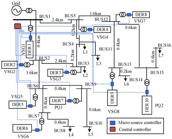
Figure 1.
The modified DongAo 10-DER 16-bus microgrid.
2.2. DER-Level TSP in Microgrids
Online TSP is an essential part of emergency control for maintaining the microgrid transient stability. The DER-level online TSP would provide comprehensive and diverse information for refined and optimized emergency control in microgrids. The specific objectives of devising the online TSP in this paper are listed as follows: (1) unstable DER identification and (2) DER’s instability severity trend prediction.
However, the transient responses of DERs are dynamically correlated in spatial and temporal dimensions, which should be considered in DER-level TSP to guarantee the prediction accuracy. This paper regards the microgrid shown in Figure 2 as an undirected graph for considering the spatial–temporal electrical data. We define the undirected graph in the time slot t as G = (Xt, E, A), where Xt is the set of all the channels detected by N VSGs, and the measured channels include the output active power P, output reactive power Q, output voltage amplitude V, and power angle δ. E is the connection relationship between each VSG. A is the adjacency matrix of G.
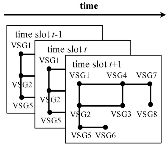
Figure 2.
The spatial–temporal graph structure for the microgrid data. Each VSG records the active power P, reactive power Q, voltage amplitude V, and power angle δ, which provide the input to the proposed model to realize the TSP.
- (1)
- Unstable DER Identification
In this paper, the graph signal for the unstable DER identification was a combination of post-fault time segments within 0.1 s and time segments within 0.1 s after the fault was cleared. The sampling frequency was 100 Hz. Thus, the time segments were 20 and the graph signal was given as X = [X1, X2, X3, …, X20], where Xt at any time slot t is expressed as follows.
The output feature shown in (2) is the transient status of the microgrid and each VSG. Here, the values of Ysys, YVSG1, YVSG2, …, YVSGN were either 0 or 1, where 1 is for the transient stability and 0 for the transient instability.
- (2)
- DER’s Instability Severity Trends Prediction
In this paper, the instability severity prediction was defined as, given G within τ time segments, to predict the transient instability severity trend of each VSG and the microgrid over the next ρ time segments. Both τ and ρ were 100 ms, and the sampling frequency was 100 Hz. Therefore, the time lengths of the input feature X and output feature Y were 10. The graph G signal was X = [X1, X2, X3, …, Xτ], where Xt on any time slot t is shown in (1) and the output feature is shown in (3).
Here, Yτ+t is expressed as follows.
where TSI is a transient stability index, which is widely used for the TSP to evaluate the degree of transient stability [37]. The calculation method of of the i-th VSG at time τ + t is shown in (5). is the power angle of the i-th VSG at time τ + t. The microgrid TSI at time τ + t is the minimum value of the TSIs of the VSGs.
2.3. Time-Varying Spatial–Temporal Dynamic Correlations
From the aforementioned introduction, time-varying spatial–temporal correlations should be incorporated into the deep learning (DL) model to improve the TSP accuracy. This part illustrates the characteristics of the time-varying spatial–temporal correlations.
- (1)
- Spatial Dynamic Correlations
During a stable operation, the correlation of DERs in the spatial dimension remains unchanged and is mainly determined by the electrical distance, load location, load level, etc. However, the spatial correlation of DERs will be changed in short-circuit faults or load level fluctuations. This means that DERs are dynamically correlated in the spatial dimension as the operating conditions are altered.
Figure 3 and Figure 4 show the spatial correlation of each VSG in the microgrid during stable and short-circuit fault states. The color of the line connecting the VSGs represents the correlation degree. As shown in Figure 3a, taking the main grid as the reference point, the VSGs automatically fall into three groups according to the electrical distance to the main grid. Figure 3b shows the power angle trajectories of the VSGs at this time, which verifies the accuracy of Figure 3a. When a short-circuit fault occurs near VSG4, the spatial correlation among the VSGs changes, and the correlation between VSG4 and VSG7, which are adjacent to the fault location, is greatly enhanced. Here, the VSGs fall into two groups: stable and unstable. Figure 4b shows the power angle trajectories of the VSGs under the fault condition. At this time, VSG3, 4, 7, and 8 represent an unstable group and VSG1, 2, 5, and 6 represent a stable group, which verifies the accuracy of Figure 4a.
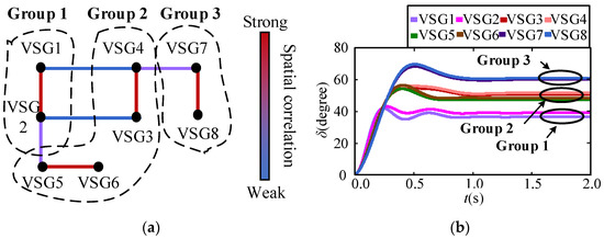
Figure 3.
Spatial correlation (a) and the power angle responses (b) of the microgrid under the normal state.

Figure 4.
Spatial correlation (a) and the power angle responses (b) of the microgrid when a short-circuit fault occurs near VSG4.
- (2)
- Temporal Dynamic Correlations
Figure 5 shows the temporal correlation of the time slots of the power angle trajectory in an unstable case, where tf is the fault moment and tc is the fault clearing moment. The power angle trend during the fault period is mainly determined by the stable operating point, fault depth, and fault duration. Thus, the contribution of point A to point C would be greater than that of point B to point C. The trend of the power angle after the fault is cleared is mainly determined by the operating point at the fault clearing time and the control dynamic of the VSG. Thus, the contribution of point A to point E would be smaller than that of point D to point E. In addition, the contribution of point A and point D for the transient stability is greater than the contribution of point B or point C, since points A and D represent the operating state of the VSG at the normal state and fault clearing moment, respectively.
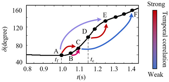
Figure 5.
Temporal correlation of the time slots of the VSG power angle trajectory in an unstable case.
In summary, the VSGs in microgrids are dynamically correlated in spatial–temporal dimensions, and the contributions of the different time slots to the transient stability are not uniform. The accuracy of DER-level TSP will deteriorate if one ignores these important interactions among DERs. Capturing and learning the complex dynamic correlations is critical to the performance of the DER-level TSP.
3. Overall Framework of the Proposed DER-Level TSP Method
The overall framework of the proposed DER-level TSP model is presented in Figure 6. It consists of m spatial–temporal convolution modules (STCMs) [21] to jointly extract the underlying time-varying spatial–temporal dynamic features of the VSGs, an unstable DER identification module (UDIM), and a DER instability severity trend prediction module (ISTPM) to achieve DER-level TSP. The detailed inner architecture and implementation process of the STCM, UDIM, and ISTPM will be explained as follows.
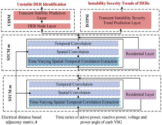
Figure 6.
Overall framework for the proposed DER-level TSP model.
3.1. STCM Architecture and Implementation Process
A STCM includes a time-varying spatial–temporal correlation extraction layer, a spatial convolution layer, and a temporal convolution layer. In addition, each STCM adopts a residential learning framework to avoid gradient disappearance and optimize the network training performance. The STCM architecture is shown in Figure 7.
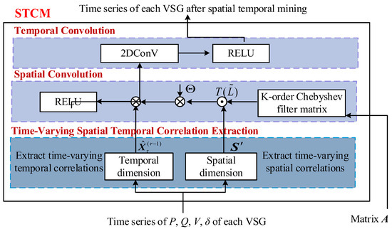
Figure 7.
STCM framework for the proposed DER-level TSP model.
- (1)
- Time-Varying Spatial–Temporal Correlation Extraction Layer
It is necessary to model the spatial information before extracting the time-varying spatial correlation. The adjacency matrix is a good solution for modeling the spatial topology in the DL model. Usually, the adjacency matrix is constructed by the connection distance. However, the electrical distance in microgrids can better reflect the correlations among DERs [28]. The electrical-distance-based adjacency matrix is calculated as follows.
First, we calculated the impedance matrix ZVSG of each VSG by (6), where Zii is the self-impedance of the i-th VSG and Zij is the mutual impedance from the i-th VSG to the j-th VSG. Then, we calculated the electrical distance EDij between any two VSGs by (7).
Finally, we normalized EDij as follows.
Thus, the adjacency matrix A based on the electrical distance is stated as follows.
- (a)
- Time-Varying Spatial Correlation Extraction
The attention mechanism proposed in [38] was adopted to capture the time-varying spatial correlations of the VSGs and adaptively assign the spatial weights among the VSGs. The calculation process is stated as follows.
Among them, is the time-varying spatial correlation matrix. is the graph data. T is the time segments. Vs, W1, W2, W3, and bs are the learning parameters of the neural network, . is the ReLU function. To ensure the fast convergence of the neural network, S was normalized by SoftMax to ensure the weights of a VSG node sum to 1.
where S′ is the output of this part. Finally, the spatial dynamic correlation matrix S′ was accompanied by the electrical distance-based adjacency matrix A to dynamically adjust the spatial weights between the VSGs in the spatial convolution layer.
- (b)
- Time-Varying Temporal Correlation Extraction
Similarly, the temporal attention mechanism was adopted to adaptively assign a correlation and importance to each time slot of the input time series. The calculation process is stated as follows.
where is the time-varying temporal correlation matrix. Vt, V1, V2, V3, and bt are the learning parameters of the neural network, . is the ReLU activation function. Similarly, the temporal attention matrix T was normalized by SoftMax.
Finally, the normalized time-varying temporal correlation matrix T′ was directly multiplied by the input X to obtain a new time series with the temporal dynamic features. is the output of this layer, which is stated as follows.
- (2)
- Spatial Convolutional Layer
The spatial convolution layer adopts a spectral domain-based graph convolution network (GCN) to mine the underlying time-varying spatial features between the VSGs [18]. The properties of the graph data were studied by calculating the eigenvalues and eigenvectors of the graph Laplacian matrix L. The mathematical representation of L is L = D − A, where D is the degree matrix of A. The normalized form of L is shown in (15), where IN is the identity matrix.
The eigenvalue decomposition expression of L is stated as follows.
where U is the Fourier basis, which is an orthogonal matrix. is the eigenvector.
We took the electrical graph data at time t as an example to perform the graph convolution. After the temporal correlation was extracted, the electrical graph signal was . Then the Fourier transform of the signal was . The essence of the GCN was to realize the graph convolution operation by replacing the classical convolution with the diagonal linear operator in the Fourier domain. Thus, using the kernel gθ to filter the electrical graph signal, the mathematical expression is stated as follows, where represents the graph convolution operation.
However, to obtain the Fourier basis, the direct eigenvalue decomposition was computationally expensive and the Chebyshev polynomials were applied to solve this problem. The approximate model for the Chebyshev polynomial is stated as follows.
In (18), , is the largest eigenvalue. K is the order of the Chebyshev polynomial. is a vector of the polynomial coefficients. Assuming that the graph electrical signal is filtered by C1 filters, then . The Chebyshev polynomial recursion is defined in (19), where .
The application of the approximate expansion of the Chebyshev polynomials to perform the graph convolution corresponded to using the kernel gθ to extract the information of the 0 to K − 1 order neighbor, i.e., the VSGs around each VSG in the graph. Each VSG was updated with the information of the 0 to K − 1 order neighbors, thereby mining the latent spatial features in the graph signal. To dynamically adjust the correlation between the VSGs, each order in the Chebyshev polynomial was combined with the time-varying spatial correlation matrix S′. The graph convolution calculation is stated in (20), where is the Hamiltonian product and the spatial convolutional layer adopts the ReLU function as the final activation function.
- (3)
- Temporal Convolutional Layer
After the spatial convolution layer captured the adjacent spatial information of each VSG, a temporal convolution layer was applied to filter the information of the adjacent temporal slots of each VSG and further extract the features in the temporal dimension. The temporal convolutional layer adopted the standard convolution. Its expression was , where * is the standard convolution operation and is the kernel parameter of the temporal convolutional layer. Assuming that was filtered using C2 filters, then . The convolution kernel size was (1, 3), that is, three time slots were combined for the convolution. Additionally, the stride was 1 and the padding was (0, 1). The activation function of the temporal convolutional layer was the ReLU function. Then, for signal , the overall formula of the spatial–temporal convolutional layer is as follows.
- (4)
- Residential Layer
The residential layer adopted the standard convolution for learning. The number of convolution filters of the residential layer was the same as that of the temporal convolution layer, i.e., C2, to ensure that the output of the residential layer had the same size as the output of the temporal convolutional layer. In addition, the convolutional kernel size was (1, 1) and the stride was (1, 1). Therefore, the size of the output of the residential layer was also (N, C2, T). Next, the output was transposed to (T, N, C2), which was activated using the ReLU function to ensure that the activation occurred at the channel dimension. Finally, the size of the output was (N, C2, T) and the output of m STCMs was the underlying feature of each VSG after spatial–temporal mining.
3.2. UDIM Architecture and the Implementation Process
The UDIM goal was to identify the unstable DERs and predict the system stability, which is a classification problem. The proposed UDIM consisted of a DER node layer and a transient stability prediction layer, as shown in Figure 8 and Figure 9. The DER node layer used a convolutional network to obtain the state of each VSG. The input size of the DER node layer was (N, C2, T), which was the output of m STCMs. The kernel size was (1, C2), the stride was (1, 1), and the filter number was 1. Thus, the convolution kernel rolled once for each VSG node to get the state of the node. The output size of the node layer was (N, 1).
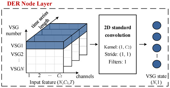
Figure 8.
DER node layer of the UDIM.
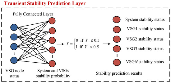
Figure 9.
Transient stability prediction layer of the UDIM.
3.3. ISTPM Architecture and the Implementation Process
The ISTPM goal was to predict the transient instability severity trend for the microgrid and each VSG, which is essentially a time series forecasting problem. The ISTPM implementation framework is shown in Figure 10.
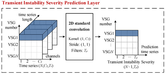
Figure 10.
Transient instability severity prediction layer of the ISTPM.
Here, we used a standard convolution layer to reduce the model parameters and improve the training effect. The ISTPM input size was (N, C2, Tτ), which was the signal X after m STCMs. The ISTPM output was . To make sure that the output result had the same dimension as that of the target, we assumed that the kernel size of this layer was (1, C2), the stride was (1, 1), and the number of filters was . Additionally, the activation function was ReLU. Thus, the instability severity trend of the VSGs and the microgrid over the next ρ time slots could be forecasted, which provide the instability ranking of the VSGs and the instability time.
4. Case Study
4.1. Simulation Setup and Dataset Generation
In this section, the modified DongAo microgrid, as shown in Figure 1, was used to verify the effectiveness and the accuracy of the proposed method. The detailed internal structures of the VSG and PQ can be found in [11].
- (1)
- Simulation Setup
The database was the basis for training the DL models. To generate the credible transient samples, this paper simulated various possible and reasonable operating transient scenarios. Corresponding numerical transient scenarios were conducted using the PSCAD/EMTDC platform v4.2.1. The simulation settings are stated as follows. (1) Nine typical load demands, including 80%, 85%, 90%, 95%, 100%, 105%, 110%, 115%, and 120% of the system-rated load power, were set up according to the system benchmark operation mode. The output power of the DERs was correspondingly changed. (2) Three-phase short-circuit faults were set on 16 buses, where the fault durations for simulating the possible transient cases included 0.1 s, 0.12 s, 0.14 s, 0.16 s, 0.18 s, and 0.2 s. (3) Considering the fault ride-through (FRT) setting, the VSG current saturation parameter was set to 1.5 and 2 times the rated current, and the PQ-controlled inverter was set to provide an active and reactive fault current, respectively. A total of 3456 transient scenarios were generated.
- (2)
- Dataset Generation
For the input features, we applied the procedure discussed in Section 2.2 to collect P, Q, V, and δ in the corresponding time segments from each transient scenario. For the output features, (1) we solved the UDI problem to determine the stability label of each transient scenario by the TSI value, which was calculated at the end of the simulation. Then, a total of 3456 UDI samples were generated. (2) For the ISTP problem, the output feature of each sample was the 0.1 s time segment after the corresponding input time segment. The previous and subsequent ISTP samples alternated for 10 ms. Then, for 3456 transient scenarios, a total of 317,952 ISTP samples were generated.
For traditional ML and DL, the general allocation ratio is 7:3 or 8:2 for the training and testing sets. In order to further accurately reflect the efficiency of the model, a more common partition ratio is 6:2:2 for the training set, validation set, and testing, which was used in this paper for the sample division. To ensure the learning performance of the neural network, we normalized the samples using z-score normalization. Accordingly, the dataset generation and preprocessing would be completed. The data processing and relevant model training and testing were conducted using Pytorch 1.11.0.
The model parameters were set as follows. In the STCMs, C1 was 64, K was 3, and C2 was 64; the number of STCMs m was 2. The iteration epoch was 50 and the learning rate was 0.001. For UDI, the loss function was cross entropy. For ISTP, the loss function was MSE.
4.2. Unstable DER Identification Performance
For the UDI problem, the model performance was evaluated as follows.
Table 1 shows the UDI performance for the proposed model, where the SVM, Naïve Bayes (NB), DBN, and spatial–temporal graph convolution network (STGCN) [23] were applied to the testing samples. The input time series of the above models were the same, but the traditional SVM, NB, and DBN methods did not contain the adjacency matrix.

Table 1.
Performance comparison of the different models in unstable DER identification.
The results showed that the proposed model achieved a 99.6% system stability prediction accuracy and a 99.0% unstable DER identification accuracy for the variable fault locations, load levels, and FRT settings. Additionally, the SVM and NB accuracies were not ideal. Specifically, the accuracy of SVM was only 60% in the unstable DER identification. Although the DBN provided a good performance in system stability prediction, the unstable DER identification accuracy was only 82.8% due to the lack of mining spatial features. The STGCN learned the spatial–temporal features and provided a performance that was better than those of the previous models. However, the STGCN could not learn the time-varying spatial–temporal correlations among the DERs; thus, its unstable DER identification accuracy was 96.3%, which was lower than that of the proposed model. The proposed model showed a superior TSP performance and captured the dynamic spatial–temporal features of the transient response.
Figure 11 shows the unstable DER identification results based on the proposed model when a fault occurred at buses 2 and 12. It can be seen that the proposed model provided accurate identification results for the unstable DERs, which was beneficial to make refined emergency control decisions after the fault.

Figure 11.
Unstable DER identification results. (a) A fault occurred at bus 2; (b) a fault occurred at bus 12.
4.3. Performance of the Instability Severity Trend Prediction
The model performance was evaluated for the instability severity trend prediction problem using the mean absolute error (MAE), root mean square error (RMSE), and mean absolute percentage error (MAPE), shown in (23)–(25). Here, and are the predicted and actual TSI values, respectively, at time τ + j in the i-th sample.
Table 2 shows the performances of the proposed model for the ISTP by applying LSTM, GRU, and STGCN on the testing samples. The input time segments were the same for all the above models, but the traditional time series models like LSTM and GRU did not contain the adjacency matrix. It can be seen that LSTM and GRUs could only mine temporal features, and their prediction performances were inferior to the STGCN, which learned the spatial–temporal features. In particular, the MAE, RMSE, and MAPE of LSTM and GRU were very large when predicting the instability severity trend of VSG4 (as shown in the table by the max MAE, max RMSE, and max MAPE). On the contrary, the STGCN and our proposed model, which incorporated the spatial features, had good prediction performances. However, the STGCN lacked the ability to learn the important time-varying spatial–temporal correlations of the DERs, thus the model performance was inferior to our proposed model.

Table 2.
Performance comparison of the different models in the instability severity trend prediction.
Since the operating data in the inverter control system could be directly collected from the MC, no additional online monitoring equipment was required at the inverter port for our proposed method. The response time was determined by the communication delay and the processing time of the proposed model. Refs. [39,40,41] have shown that in a centralized microgrid, the communication delay between MC and CC was at the millisecond level. In addition, the PC was configured as an Intel(R) Core (TM) i5-10400F CPU/16.00 GB RAM, Intel (China) Co., Beijing, China. Under this configuration, the UDI processing time of the proposed model was 20.85 ms and the ISTP processing time was 10.04 ms. The instability time scale of the transient stability problem of the microgrid was in the order of hundreds of milliseconds, and the fastest instability time among all the generated 3456 transient scenarios was 263 ms. Therefore, the response time of the model met the requirements of the TSP for microgrids.
In this paper, if the power angle varied between 90° and 360°, that is, the TSI was within 0 to 0.6, then, the VSG was in an emergency state. If the TSI was less than 0, the VSG was in an unstable state. Figure 12 shows the instability severity trend prediction results of the proposed model under stable and unstable samples. Figure 13 shows the predicted instability severity trends of all the VSGs when a fault occurred at buses 2 and 12. The solid line is the actual TSI, and the dotted line is the predicted TSI. It can be seen that the proposed model had a strong time series prediction capability, which precisely predicted the transient instability severity trends of all the VSGs. Thus, the proposed model provided a ranking of the instability severity and the instability time of each VSG. The proposed results can further help grid operators prioritize DERs as control objects in a refined emergency control strategy.

Figure 12.
ISTP performance; (a) stable case, (b) unstable case.
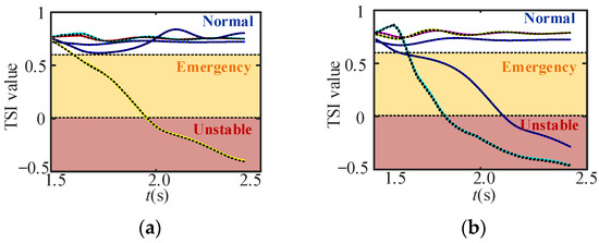
Figure 13.
ISTP performance of eight VSGs; (a) a fault at bus 2, (b) a fault at bus 12.
4.4. Effectiveness of Time-Varying Spatial–Temporal Correlations Extraction
- (1)
- Time-Varying Spatial Correlation Extraction
As mentioned above, the VSG reference power, load position, load level, and fault location are the influencing factors in spatial correlations. Therefore, this part set the output power of each VSG to 80 kW and assumed a fixed load quantity and access point to measure the effectiveness of the time-varying spatial correlation extraction. By changing the fault duration and location, a total of 7380 ISTP samples were generated. Then, we found the average of the matrix S′ for the generated test samples whose fault location was at bus 6 (fault near VSG5), as displayed in Figure 14a.
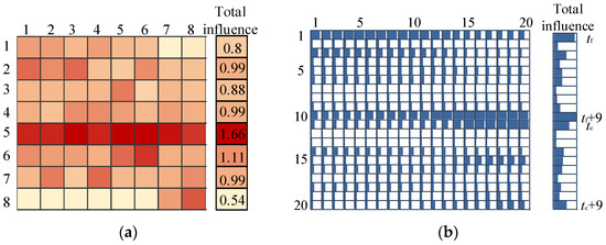
Figure 14.
Spatial and temporal dynamic correlation visualization. (a) Spatial dynamic correlation visualization; (b) temporal dynamic correlation visualization.
In Figure 14a, white represents a weak correlation and dark red represents a strong correlation. The color of the i-th row and j-th column represents the influence of the i-th VSG on the j-th VSG. The sum of the i-th column is 1. The sum of the i-th row reflects the total influence of the VSG on the transient stability. The total influence is tabulated in the right column of Figure 14a.
It can be seen that when the fault occurred near VSG5, the influence of VSG5 on the other VSGs and its total influence were the greatest. This was reasonable because VSG5 suffered the most from the disturbance and its power angle rose the fastest, which significantly affected the transient stability of the other VSGs. In addition, VSG8 was only correlated with VSG7. This was consistent with the actual situation since VSG8 was spatially close to VSG7 and apart from VSGs 1–6. Thus, the spatial dynamic correlation matrix effectively reflected the spatial dynamic correlation of the VSGs and signified the impact of each VSG on the transient stability.
- (2)
- Time-Varying Temporal Correlation Extraction
To visually verify the effectiveness of the time-varying temporal correlation extraction mechanism, this part averaged the matrix T′ of the UDI test samples and displayed the proportion of T′ in the form of a data bar, as shown in Figure 14b.
In the figure, the value in the i-th row and the j-th column represents the influence of the i-th time slot on the j-th time slot. The sum of the i-th row reflects the total contribution of the i-th time slot to stability.
Here, tf, tf + 9 (i.e., the last sampling point during the fault period), tc, and tc + 9 (i.e., the last sampling point after fault clearing) had the greatest impacts on the transient stability, which was reasonable because the values at tf reflected the operating point at the steady state. The values at tf + 9 were the sampled maximum or minimum values during the fault, which reflected the fault degree, and the values at tc reflected the operating point of the VSG after the fault was cleared. The values at tf + 9 reflected whether the VSG entered the power angle deceleration stage. In addition, the influence of tf on time slots 1–20 showed a descending trend and the influence of tf + 9, tc, and tc + 9 on time slots 1–20 increased gradually. This was reasonable since the transient response during the fault was mainly determined by the stable operating point and the fault degree. Additionally, the transient response once the fault was cleared was mainly determined by the operating point at the fault clearing moment and fault degree.
Accordingly, it can be concluded that T′ effectively reflected the dynamic correlation between the time slots and the contribution of each time slot to the transient stability.
4.5. Effectiveness of the Spatial–Temporal Convolution Module
To verify the STCM performance, the original data of the 3456 unstable DER identification samples, outputs of STCM 1, outputs of STCM 2, and outputs of the DER node layer were analyzed using t-distributed stochastic neighbor embedding (t-SNE) for the visualization of the feature extraction capability of each layer.
Figure 15 shows the t-SNE visualization results of the raw data, the output data of STCM 1, the output data of STCM 2, and the output data of the DER node layer. It can be seen that the stable and unstable samples in the original raw data were mixed. After passing them through STCM 1 and STCM 2, the distinction between the stable and unstable situations gradually increased. After the DER node layer, the stable samples and unstable samples were basically divided into two clusters in terms of location. This demonstrated the STCM’s excellent feature extraction capability for predicting the transient stability.

Figure 15.
t-SNE visualization of the data in each layer. (a) Visualization results of the raw data, (b) visualization results of the output data of STCM 1, (c) visualization results of the output data of STCM 2, (d) visualization results of the output data of the DER node layer.
4.6. Adaptive Testing in an Unknown Scenario
In this section, new transient scenarios were generated to verify the performance of the proposed model in unknown scenarios. The settings were as follows. The load level was set to 125% and the fault location, fault durations, and FRT strategy were the same as those in Section 4.1. For the unstable DER identification, a total of 384 samples were generated and a total of 35,328 samples were generated for the instability severity trend prediction. Using the model presented in Section 4.2 and Section 4.3, the performances in the unknown scenario were calculated and shown in Table 3 and Table 4.

Table 3.
Unstable DER identification performance in unknown scenarios.

Table 4.
Instability severity trend prediction performance in unknown scenarios.
Here, the proposed model still achieved a good prediction performance, which showed that the proposed model could well adapt to transient events which were not covered by the initial scenario.
5. Conclusions
The complex spatial–temporal dynamic correlations among DERs make it difficult to maintain the reliability and the accuracy of the DER-level transient analysis in microgrids. This paper proposed a novel DER-level transient stability prediction method, which was based on spatial–temporal graph convolution networks, to provide precise unstable DER identification and quantitative instability severity trends for DERs. The proposed model consisted of several stacked spatial–temporal convolution modules (STCMs), an unstable DER identification module (UDIM), and an instability severity trend prediction module (ISTPM). The stacked STCMs automatically extracted the time-varying spatial–temporal correlations and simultaneously learned the spatial–temporal transient features underlying the transient graph data of the DERs. The UDIM identified the unstable DERs and analyzed the microgrid stability. The ISTPM provided the instability severity trends of the DERs and gave the instability DER ranking and the instability time of the DERs. The test results showed that the proposed method greatly improved the DER-level TSP performance of microgrids under various fault locations, load levels, and fault ride-through settings. In addition, the time-varying spatial–temporal correlation extraction mechanism automatically captured and assigned dynamic correlations among the DERs, giving the model an interpretability advantage. These predicted results provided abundant information to achieve refined and cost-efficient emergency control in microgrids.
The occurrence probability of asymmetric faults was higher than that of the symmetric faults in practical applications. In the future, the transient stability prediction methods for microgrids under asymmetric disturbance or short-circuit faults need to be explored.
Author Contributions
Methodology, H.Z. and L.H. (Lili He); Project administration, L.H. (Lili He); Supervision, Y.P.; Resources, Z.S.; Supervision, Z.Z.; Supervision, L.H. (Liang Hu); Writing—original draft, H.Z. All authors have read and agreed to the published version of the manuscript.
Funding
This research was funded by National Natural Science Foundation of China under Grant 52125705, the fellowship of China Postdoctoral Science Foundation 2022M721082, and the National Natural Science Foundation of China under Grant 52107194.
Data Availability Statement
The data presented in this study are available on request from the corresponding author.
Conflicts of Interest
Authors Huimin Zhao, Zhixue Zhang and Liang Hu were employed by the company CRRC Zhuzhou Electric Locomotive Institute Co., Ltd. The remaining authors declare that the research was conducted in the absence of any commercial or financial relationships that could be construed as a potential conflict of interest.
References
- Kabalan, M.; Singh, P.; Niebur, D. Large Signal Lyapunov-Based Stability Studies in Microgrids: A Review. IEEE Trans. Smart Grid 2017, 8, 2287–2295. [Google Scholar] [CrossRef]
- Shen, C.; Shuai, Z.; Shen, Y.; Peng, Y.; Liu, X.; Li, Z.; Shen, Z.J. Transient Stability and Current Injection Design of Paralleled Current-Controlled VSCs and Virtual Synchronous Generators. IEEE Trans. Smart Grid 2021, 12, 1118–1134. [Google Scholar] [CrossRef]
- Huang, T.; Gao, S.; Xie, L. A Neural Lyapunov Approach to Transient Stability Assessment of Power Electronics-Interfaced Networked Microgrids. IEEE Trans. Smart Grid 2022, 13, 106–118. [Google Scholar] [CrossRef]
- Li, F.; Wang, Q.; Tang, Y.; Xu, Y.; Dang, J. Hybrid analytical and data-driven modeling based instance-transfer method for power system online transient stability assessment. CSEE J. Power Energy Syst. 2021; early access. [Google Scholar] [CrossRef]
- Li, X.; Yang, Z.; Guo, P.; Cheng, J. An Intelligent Transient Stability Assessment Framework with Continual Learning Ability. IEEE Trans. Industr. Inform. 2021, 17, 8131–8141. [Google Scholar] [CrossRef]
- Zhao, T.; Wang, J.; Lu, X.; Du, Y. Neural Lyapunov Control for Power System Transient Stability: A Deep Learning-Based Approach. IEEE Trans. Power Syst. 2022, 37, 955–966. [Google Scholar] [CrossRef]
- Pico, H.N.V.; Johnson, B.B. Transient Stability Assessment of Multi-Machine Multi-Converter Power Systems. IEEE Trans. Power Syst. 2019, 34, 3504–3514. [Google Scholar] [CrossRef]
- La Scala, M.; Sbrizzai, R.; Torelli, F.; Scarpellini, P. A tracking time domain simulator for real-time transient stability analysis. IEEE Trans. Power Syst. 1998, 13, 992–998. [Google Scholar] [CrossRef]
- Zhang, Y.; Xie, L. A Transient Stability Assessment Framework in Power Electronic-Interfaced Distribution Systems. IEEE Trans. Power Syst. 2016, 31, 5106–5114. [Google Scholar] [CrossRef]
- Alipoor, J.; Miura, Y.; Ise, T. Stability Assessment and Optimization Methods for Microgrid with Multiple VSG Units. IEEE Trans. Smart Grid 2018, 9, 1462–1471. [Google Scholar] [CrossRef]
- Zhao, H.; Peng, Y.; Shuai, Z.; Zhao, F.; Shen, X. Online transient stability prediction method of microgrid considering different distributed energy resources’ interaction under current saturation. CSEE J. Power Energy Syst. 2023; early access. [Google Scholar] [CrossRef]
- Wang, B.; Fang, B.; Wang, Y.; Liu, H.; Liu, Y. Power System Transient Stability Assessment Based on Big Data and the Core Vector Machine. IEEE Trans. Smart Grid 2016, 7, 2561–2570. [Google Scholar] [CrossRef]
- You, D.; Wang, K.; Ye, L.; Wu, J.; Huang, R. Transient stability assessment of power system using support vector machine with generator combinatorial trajectories inputs. Int. J. Electr. Power Energy Syst. 2013, 44, 318–325. [Google Scholar] [CrossRef]
- Moulin, L.S.; da Silva, A.P.A.; El-Sharkawi, M.A.; Marks, R.J. Support vector machines for transient stability analysis of large-scale power systems. IEEE Trans. Power Syst. 2004, 19, 818–825. [Google Scholar] [CrossRef]
- Gomez, F.R.; Rajapakse, A.D.; Annakkage, U.D.; Fernando, I.T. Support Vector Machine-Based Algorithm for Post-Fault Transient Stability Status Prediction Using Synchronized Measurements. IEEE Trans. Power Syst. 2011, 26, 1474–1483. [Google Scholar] [CrossRef]
- Amraee, T.; Ranjbar, S. Transient Instability Prediction Using Decision Tree Technique. IEEE Trans. Power Syst. 2013, 28, 3028–3037. [Google Scholar] [CrossRef]
- Sun, K.; Likhate, S.; Vittal, V.; Kolluri, V.S.; Mandal, S. An Online Dynamic Security Assessment Scheme Using Phasor Measurements and Decision Trees. IEEE Trans. Power Syst. 2007, 22, 1935–1943. [Google Scholar] [CrossRef]
- He, M.; Zhang, J.; Vittal, V. Robust Online Dynamic Security Assessment Using Adaptive Ensemble Decision-Tree Learning. IEEE Trans. Power Syst. 2013, 28, 4089–4098. [Google Scholar] [CrossRef]
- Xu, Y.; Dong, Z.Y.; Zhao, J.H.; Zhang, P.; Wong, K.P. A Reliable Intelligent System for Real-Time Dynamic Security Assessment of Power Systems. IEEE Trans. Power Syst. 2012, 27, 1253–1263. [Google Scholar] [CrossRef]
- Zhang, R.; Xu, Y.; Dong, Z.; Wong, K. Post-disturbance transient stability assessment of power systems by a self-adaptive intelligent system. IET Gener. Trasm. Dis. 2015, 9, 296–305. [Google Scholar] [CrossRef]
- Guo, S.; Lin, Y.; Feng, N.; Song, C.; Wan, H. Attention Based Spatial-Temporal Graph Convolutional Networks for Traffic Flow Forecasting. In Proceedings of the AAAI Conference on Artificial Intelligence, Honolulu, HI, USA, 27 January–1 February 2019; Volume 33, pp. 922–929. [Google Scholar]
- Yu, X.; Gao, F.; Ding, G. Deep Learning Based Transient Stability Assessment for Grid-Connected Inverter. In Proceedings of the 2018 IEEE International Power Electronics and Application Conference and Exposition (PEAC), Shenzhen, China, 4–7 November 2018; pp. 1–5. [Google Scholar]
- Zhu, L.; Hill, D.J.; Lu, C. Hierarchical Deep Learning Machine for Power System Online Transient Stability Prediction. IEEE Trans. Power Syst. 2020, 35, 2399–2411. [Google Scholar] [CrossRef]
- Bahbah, A.G.; Girgis, A.A. New method for generators’ angles and angular velocities prediction for transient stability assessment of multimachine power systems using recurrent artificial neural network. IEEE Trans. Power Syst. 2004, 19, 1015–1022. [Google Scholar] [CrossRef]
- Li, B.; Wu, J.; Hao, L.; Shao, M.; Zhang, R.; Zhao, W. Anti-Jitter and Refined Power System Transient Stability Assessment Based on Long-Short Term Memory Network. IEEE Access 2020, 8, 35231–35244. [Google Scholar] [CrossRef]
- Shen, Y.; Peng, Y.; Shuai, Z.; Zhou, Q.; Zhu, L.; Shen, Z.J. Hierarchical Time-Series Assessment and Control for Transient Stability Enhancement in Islanded Microgrids. IEEE Trans. Smart Grid 2023, 14, 3362–3374. [Google Scholar] [CrossRef]
- Yan, R.; Geng, G.; Jiang, Q.; Li, Y. Fast transient stability batch assessment using cascaded convolutional neural networks. IEEE Trans. Power Syst. 2019, 33, 3510–3520. [Google Scholar] [CrossRef]
- Huang, J.; Guan, L.; Su, Y.; Yao, H.; Guo, M.; Zhong, Z. Recurrent Graph Convolutional Network-Based Multi-Task Transient Stability Assessment Framework in Power System. IEEE Access 2020, 8, 93283–93296. [Google Scholar] [CrossRef]
- Seo, Y.; Michael, D.; Pierre, V.; Bresson, X. Structured sequence modeling with graph convolutional recurrent networks. arXiv 2016, arXiv:1612.07659. [Google Scholar]
- Yu, B.; Yin, H.; Zhu, Z. Spatio-Temporal Graph Convolutional Networks: A Deep Learning Framework for Traffic Forecasting. arXiv 2018, arXiv:1709.04875. [Google Scholar]
- Luo, Y.; Lu, C.; Zhu, L.; Song, J. Data-driven short-term voltage stability assessment based on spatial-temporal graph convolutional network. Int. J. Electr. Power Energy Syst. 2021, 130, 106753. [Google Scholar] [CrossRef]
- Zhu, L.; Wen, W.; Li, J.; Hu, Y. Integrated Data-Driven Power System Transient Stability Monitoring and Enhancement. IEEE Trans. Power Syst. 2023; early access. [Google Scholar] [CrossRef]
- Zhao, Z.; Yang, P.; Guerrero, J.M.; Xu, Z.; Green, T.C. Multiple-Time-Scales Hierarchical Frequency Stability Control Strategy of Medium-Voltage Isolated Microgrid. IEEE Trans. Power Electron. 2016, 31, 5974–5991. [Google Scholar] [CrossRef]
- Abdelgayed, T.S.; Morsi, W.G.; Sidhu, T.S. A New Approach for Fault Classification in Microgrids Using Optimal Wavelet Functions Matching Pursuit. IEEE Trans. Smart Grid 2018, 9, 4838–4846. [Google Scholar] [CrossRef]
- Chanda, S.; Srivastava, A.K. Defining and Enabling Resiliency of Electric Distribution Systems with Multiple Microgrids. IEEE Trans. Smart Grid 2016, 7, 2859–2868. [Google Scholar] [CrossRef]
- Kaur, A.; Kaushal, J.; Basak, P. A review on microgrid central controller. Renew. Sust. Energ. Rev. 2016, 55, 338–345. [Google Scholar] [CrossRef]
- Zhu, L.; Hill, D.J. Networked Time Series Shapelet Learning for Power System Transient Stability Assessment. IEEE Trans. Power Syst. 2022, 37, 416–428. [Google Scholar] [CrossRef]
- Feng, X.; Guo, J.; Qin, B.; Liu, T.; Liu, Y. Effective deep memory networks for distant supervised relation extraction. In Proceedings of the International Joint Conference on Artificial Intelligence (IJCAI), Melbourne, Australia, 19–25 August 2017; Volume 17, pp. 19–25. [Google Scholar]
- Díaz, N.L.; Luna, A.C.; Vasquez, J.C.; Guerrero, J.M. Centralized Control Architecture for Coordination of Distributed Renewable Generation and Energy Storage in Islanded AC Microgrids. IEEE Trans. Power Electron. 2017, 32, 5202–5213. [Google Scholar] [CrossRef]
- Utkarsh, K.; Srinivasan, D.; Trivedi, A.; Zhang, W.; Reindl, T. Distributed Model-Predictive Real-Time Optimal Operation of a Network of Smart Microgrids. IEEE Trans. Smart Grid 2019, 10, 2833–2845. [Google Scholar] [CrossRef]
- Setiawan, M.A.; Shahnia, F.; Rajakaruna, S.; Ghosh, A. ZigBee-Based Communication System for Data Transfer Within Future Microgrids. IEEE Trans. Smart Grid 2015, 6, 2343–2355. [Google Scholar] [CrossRef]
Disclaimer/Publisher’s Note: The statements, opinions and data contained in all publications are solely those of the individual author(s) and contributor(s) and not of MDPI and/or the editor(s). MDPI and/or the editor(s) disclaim responsibility for any injury to people or property resulting from any ideas, methods, instructions or products referred to in the content. |
© 2024 by the authors. Licensee MDPI, Basel, Switzerland. This article is an open access article distributed under the terms and conditions of the Creative Commons Attribution (CC BY) license (https://creativecommons.org/licenses/by/4.0/).