Powering Electricity Forecasting with Transfer Learning

Abstract

Accurate forecasting is one of the keys to the efficient use of the limited existing energy resources and plays an important role in sustainable development. While most of the current research has focused on energy price forecasting, very few studies have considered medium-term (monthly) electricity generation. This research aims to fill this gap by proposing a novel forecasting approach based on zero-shot transfer learning. Specifically, we train a Neural Basis Expansion Analysis for Time Series (NBEATS) model on a vast dataset comprising diverse time series data. Then, the trained model is applied to forecast electric power generation using zero-shot learning. The results show that the proposed method achieves a lower error than the benchmark deep learning and statistical methods, especially in backtesting. Furthermore, the proposed method provides vastly superior execution time as it does not require problem-specific training.

1. Introduction

Limited natural resources, coupled with an incessantly growing global demand for energy, have given rise to an unsustainable situation. As the world’s population continues to expand, the need for fuel and energy has skyrocketed. Of particular concern is the rapid rise in demand for electricity, in part driven by the widespread adoption of electric cars and other environmentally friendly alternatives. The limited capacity for electricity generation necessitates careful planning and efficient production to meet these escalating demands.

Efficiency in power distribution and utilization hinges upon the accurate forecasting of future supply and demand. The ability to forecast electricity generation accurately and in a timely manner enables utilities to maximize the utilization of available resources. As a result, forecasting electricity generation has become an imperative task in modern industrialized societies. However, the increasing integration of renewable energy sources into today’s power systems has introduced greater volatility into electricity generation. Despite an extensive body of literature dedicated to forecasting electricity prices, few recent studies have addressed the specific challenge of forecasting electricity generation. This research aims to fill this gap by proposing a novel approach to forecasting electric power generation based on transfer learning.

The existing approaches to energy forecasting can be grouped into three main categories: statistical, deep learning, and hybrid methods. Statistical methods employ autoregressive models to construct forecasts. While statistical methods are capable of producing accurate forecasts, they are slow to compute and require significant execution time. Deep learning approaches utilize a plethora of deep learning models to perform forecasts. While deep learning models have produced accurate results in some cases, they are not well-suited for energy-related forecasts due to the lack of data. It is well known that deep learning thrives with big data. Since time series data in energy domains are limited, it is not sufficient to fully train deep learning models. Finally, hybrid models combine two or more methods to design a multi-step forecasting model. While these approaches may work in special cases, they are difficult to generalize. Recently, transfer learning has shown immense potential to accelerate the training process and improve accuracy.

Transfer learning, a powerful technique for training deep learning models, has proven successful in various domains, such as computer vision, speech recognition, and large language models. However, its application within the context of electric power forecasting has been limited. In this paper, we propose a forecasting model based on transfer learning principles. In particular, we employ a hitherto unexplored approach based on zero-shot learning in order to achieve minimum execution time. Unlike traditional transfer learning paradigms, zero-shot learning does not require additional fine-tuning of the pretrained base model, which leads to a more efficient and flexible model. To implement our strategy, we utilize the Neural Basis Expansion Analysis for Time Series (NBEATS) model on a vast dataset comprising diverse time series data. The trained model is applied to forecast electric power generation using zero-shot learning.

Transfer learning has emerged to tackle the issue of effectively training deep learning models in the regime of limited data availability. The core idea of transfer learning is to pretrain a model on an extremely large dataset and then fine-tune the trained model on the specific task using an additional, smaller dataset. Since recurrent models that process data in a sequential manner are notoriously slow to train, they are not well suited for transfer learning. On the other hand, the NBEATS model consists of fully connected blocks with residual connections that are fast to train. Consequently, it is better suited for transfer learning than recurrent models.

By adopting a transfer learning approach, we leverage the knowledge and patterns extracted from different domains to enhance the accuracy and efficiency of forecasting electricity generation. This research seeks to explore the untapped potential of transfer learning in addressing the challenges posed by the volatile nature of modern power systems. In addition, by employing zero-shot learning, we are able to provide fast prediction with no context-specific training.

The main contributions of this research are as follows:

• Novel forecasting framework based on zero-shot transfer learning;
• Improved accuracy in forecasting electricity generation;
• Superior execution time.

The remainder of this paper is organized as follows: Section 2 provides an overview of the related work in electricity generation forecasting and transfer learning. Section 3 details the proposed forecasting model and the methodology employed. Section 4 discusses the results obtained from our experiments, and Section 5 concludes the paper with a summary of findings and suggestions for future research.

2. Literature

Time series forecasting in general and electricity forecasting in particular have attracted a tremendous amount of attention over the last decade [1]. The existing research related to power forecasting can be grouped into three categories: (1) statistical models, (2) deep learning models, and (3) hybrid models. Statistical approaches are based on autoregressive linear regression models. Deep learning models are based on various types of neural networks that employ a lookback window to produce forecasts. Hybrid models combine two or more methods to create a single forecast. Electricity forecasting can be further grouped into short-, medium-, and long-term forecasting, as well as univariate and multivariate forecasting.

2.1. Statistical Models

Traditional statistical techniques remain popular approaches to electricity forecasting. In most cases, the time series is modeled via an autoregressive linear regression model. The series’ past values (input) are employed to predict its future values (output). Least squares linear regression, maximum likelihood estimation, and autoregressive moving average methods are common methods for estimating model parameters. Recently, linear regression models with a large number of input features that employ regularization techniques have risen to prominence. The most commonly used regularization method is the least absolute shrinkage and selection operator (LASSO), which minimizes the $L_1$ norm of the feature vector, and has been shown to improve the model’s performance [2,3]. Another development has been the application of additional preprocessing techniques such as variance stabilizing transformations [4] and long-term seasonal components [5]. In addition, ensemble methods that combine multiple forecasts of the same model calibrated on different windows have also become popular [6]. Ensemble algorithms based on a statistical analysis of the forecast error, signal shape, and difference of derivatives in joint points have been used to forecast current and voltage time series [7]. Finally, we note that unlike financial time series forecasting, where generalized autoregressive conditional heteroskedastic (GARCH) models are ubiquitous, electricity forecasting is more accurate using the basic autoregressive (AR) and autoregressive integrated moving average (ARIMA) models [8,9].

2.2. Deep Learning Models

Deep learning is used extensively in time series forecasting. The main workhorse has been the recurrent neural network (RNN) and its extensions such as gated recurrent units (GRUs) and long short-term memory (LSTM) networks. The RNN model is designed specifically for sequence-to-sequence modeling, where the output in the next time step is based on the current input as well as the previous output [10]. A large number of studies have used LSTM, whose architecture is designed to reduce the issue of the vanishing gradient signal, as the core forecasting model with varying degrees of success [11,12,13].

Convolutional neural networks (CNNs) have also been employed in time series forecasting. Notably, the temporal convolutional network (TCN) has been a popular forecasting model in various applications, including electricity forecasting [14]. The TCN model consists of three main components: causal convolutions, dilated convolutions, and residual connections. More recently, pure deep learning models based on stacked fully connected layers have shown impressive results. The NBEATS model showed state-of-the-art performance on several well-known datasets, including M3, M4, and TOURISM competition datasets containing time series from diverse domains [15]. Its architecture employs backward and forward residual links and a very deep stack of fully connected layers. It has several desirable properties: being interpretable, applicable without modification to a wide array of target domains, and fast to train. A similar model, Neural Hierarchical Interpolation for Time Series Forecasting (NHiTS), showed even greater accuracy on a wide range of forecasting tasks, including electricity forecasting [16].

2.3. Hybrid Models

Over the last several years, there has been an explosion of hybrid forecasting models, which comprise at least two of the following five modules [1]:

• Decomposing data [17,18];
• Feature selection [19,20];
• Clustering data [21];
• One or more forecasting models whose predictions are combined [22,23];
• A heuristic optimization algorithm to either estimate the models or their hyperparameters [24].

By combining two or more different techniques, researchers aim to overcome the deficiencies of individual components. The drawbacks of hybrid approaches include increased computing time and increased model complexity, which hinders model interpretability.

2.4. Transfer Learning

There are several studies that employ transfer learning in energy forecasting. Existing methods use traditional transfer learning techniques, where a model is pretrained on external (source) data that are similar to the target data. Then, the target data are used to fine-tune the model [25,26,27,28,29]. In [25], the authors employed a conventional approach to transfer learning. First, a CNN model is pretrained on public data that are similar to the target data. Then, the last layers of the model are retrained using the target training data. A similar approach is employed in [26], where a model is pretrained using external data that are similar to the target data. Then, the target data are doubled via a generative adversarial network to increase the size of the target training data. Finally, the last layers of the model are retrained using the enlarged target data. Furthermore, in [27], the authors explored three different transfer learning strategies: (1) retraining only the last hidden layer, (2) using the pretrained model to initialize the weights of the final model, and (3) retraining the last hidden layer from scratch. Sequential transfer learning, where the time frame of the source data precedes that of the target data, was explored in [30].

Another approach to using transfer knowledge from external data is based on data augmentation. In [31], the authors propose a transfer learning approach called Hephaestus designed for cross-building energy forecasting. In this approach, the information from other buildings (source) is used together with the target building to train a forecasting model. Since both the source and target information is used simultaneously to train the model, this approach is akin to augmenting the training data. Other innovative approaches include chain transfer learning, where multiple models are trained in sequence. In [32], the authors use chain-based transfer learning to forecast several energy meters. In this approach, the first meter is trained traditionally using RNN. The model for the next meter starts the training process with the pretrained model from the first meter. The process continues in a chain-like manner.

2.5. Medium-Term Forecasting

Monthly energy forecasting has received considerably less attention than short-term forecasting. In particular, we found only one recent study [33] that provided multi-month forecasting using transfer learning. The majority of the existing studies produce forecasts over short-term horizons [34]: hourly [25,27,28] or daily [26,29,30,31]. Even in an expanded scope considering general deep learning techniques for energy forecasting, only a few studies were found to carry out monthly predictions. In [35], the authors compared the performance of LSTM to neural networks and CNN for monthly energy consumption prediction.

The review of the literature shows a lack of transfer learning methods based on zero-shot learning. Given the recent success of zero-shot learning [36], this offers a promising new avenue for research in energy forecasting. In addition, the literature analysis shows that existing models use only domain-related data to pretrain the models. We propose expanding the source data used in pretraining to include a wide range of time series from various domains. In this way, we expand the amount of available training data, which is crucial in building effective deep learning models [37].

3. Methodology

In this section, we provide details of the proposed approach to power forecasting. First, we present the underlying concepts, including transfer learning, meta-learning, and the NBEATS model. Then, we describe the use of transfer learning, together with the NBEATS model, to construct a zero-shot forecasting model.

3.1. Transfer Learning

Transfer learning is a machine learning technique where knowledge gained from solving one problem is applied to another related problem. Rather than starting from scratch, a pretrained model is used as a starting point, and its learned features are used to improve performance on a new task. More formally, transfer learning can be described in terms of domains and tasks. A domain $\mathcal{D}$ consists of a features space $\mathcal{X}$ and a marginal distribution $P\left(X\right)$, where $X=\{x_1,x_2,\dots ,x_n\}\in \mathcal{X}$. For a given domain $\mathcal{D}$, a task $\mathcal{T}$ consists of a label space $\mathcal{Y}$ and a predictive function $f:\mathcal{X}\to \mathcal{Y}$. The predictive function is used to assign labels to new instances of x, and it is learned from the training set $x_i\in X, y_i\in \mathcal{Y}$. Given source domain ${\mathcal{D}}_S$ and source task ${\mathcal{T}}_S$, a target domain ${\mathcal{D}}_T$, and target task ${\mathcal{T}}_T$, transfer learning aims to improve the learning of the target predictive function $f_T(·)$ using the knowledge of ${\mathcal{D}}_S$ and ${\mathcal{T}}_S$ [38].

In the context of neural networks, transfer learning is often used to fine-tune a general-purpose model trained on a large dataset to perform a new task with minimal additional training. It is employed in multiple applications. In image classification, a model that was pretrained on a large image dataset such as ImageNet can recognize various objects including cars, dogs, and trees. This pretrained model can be used as a starting point for a new image classification task. By leveraging the pretrained model’s knowledge of visual features, the model can quickly adapt to the new task and achieve better accuracy with fewer training data. Recently, transfer learning has been used successfully in natural language processing. Large language models such as generative pretrained transformer (GPT) and bidirectional encoder representations from transformers (BERT) are pretrained on a large corpus of text data, learning the contextual relationships between words, which can then be fine-tuned on specific downstream tasks such as sentiment analysis, question answering, or named entity recognition [39,40,41].

3.2. Meta-Learning

Meta-learning or learning-to-learn is a subfield of transfer learning that has recently risen to prominence. It is usually linked to being able to accumulate knowledge across tasks and quickly adapt the accumulated knowledge to the new task (task adaptation) [42]. The meta-learning process is divided into two stages: meta-training and meta-testing. During meta-training, a model is exposed to a diverse set of training tasks or domains. The model learns to extract relevant features, adapt its parameters, or develop strategies that can be generalized to new tasks. The goal is to learn a set of initial parameters or representations that are well-suited for a wide range of tasks.

In the context of time series, a meta-learning procedure can generally be viewed at two levels: the inner loop and the outer loop. The inner training loop operates within an individual meta-example or task $\mathcal{T}$ and represents the fast learning loop, improving over current $\mathcal{T}$ [43]. The outer loop operates across tasks and represents a slow learning loop. A task $\mathcal{T}$ includes task training data ${\mathcal{D}}_{\mathcal{T}}^{tr}$ and task validation data ${\mathcal{D}}_{\mathcal{T}}^{val}$, both optionally involving inputs, targets, and a task-specific loss: ${\mathcal{D}}_{\mathcal{T}}^{tr}:\{{\mathcal{X}}_{\mathcal{T}}^{tr},{\mathcal{Y}}_{\mathcal{T}}^{tr},{\mathcal{L}}_{\mathcal{T}}\},{\mathcal{D}}_{\mathcal{T}}^{val}:\{{\mathcal{X}}_{\mathcal{T}}^{val},{\mathcal{Y}}_{\mathcal{T}}^{val},{\mathcal{L}}_{\mathcal{T}}\}$. Accordingly, a meta-learning set-up can be defined by assuming a distribution $p\left(\mathcal{T}\right)$ over tasks, a predictor ${\mathcal{P}}_{\theta }$, and a meta-learner with meta-parameters $\varphi$. The objective is to design a meta-learner that can generalize well on a new task by appropriately choosing the predictor’s task-adaptive parameters $\theta$ after observing ${\mathcal{D}}_{\mathcal{T}}^{tr}$ [43].

The best-case scenario in meta-learning is zero-shot learning, where the model is not trained on the target dataset. Zero-shot learning is the model’s ability to make predictions using unseen data, without having specifically trained on them. In the case of time series forecasting, there are often not enough data to train a model even using transfer learning. Therefore, zero-shot learning offers a viable approach to applying deep learning to time series forecasting.

3.3. NBEATS

The Neural Basis Expansion Analysis for Time Series is a powerful deep learning model designed for time series forecasting that has demonstrated outstanding performance on several competition benchmarks [15]. It is a framework that combines interpretable components with neural networks to capture and forecast complex temporal patterns. NBEATS decomposes the time series into a set of basis functions and combines them to make accurate predictions.

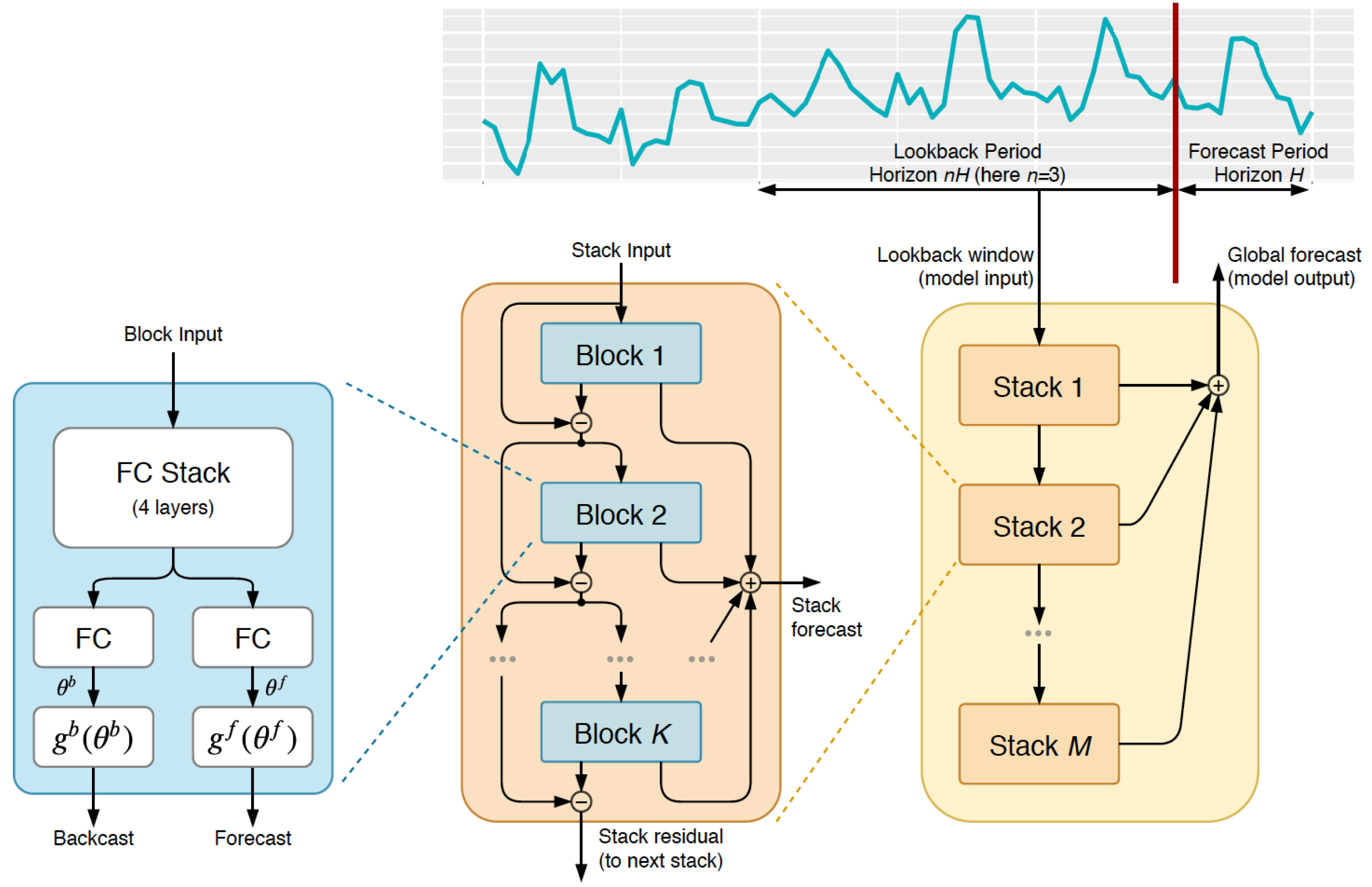
As shown in Figure 1, the NBEATS model consists of a sequence of stacks, where each stack contains K blocks that are connected by a doubly residual architecture. A given block l has one input ${\mathbf{x}}_l$ and two outputs: the backcast ${\widehat{\mathbf{x}}}_l$ and the partial forecast ${\widehat{\mathbf{y}}}_l$. In the initial block, we set ${\mathbf{x}}_1\equiv \mathbf{x}$, where $\mathbf{x}$ denotes the model-level input. We define the k-th fully connected layer in the l-th block, having ReLU non-linearity, weights ${\mathbf{W}}_k$, bias ${\mathbf{b}}_k$, and input ${\mathbf{h}}_{l,k-1}$, as ${\mathrm{FC}}_k\left({\mathbf{h}}_{l,k-1}\right)\equiv \mathrm{ReLU}({\mathbf{W}}_k{\mathbf{h}}_{l,k-1}+{\mathbf{b}}_k)$. In the configuration that shares all the learnable parameters across blocks, NBEATS is described as follows [15,43]:

$$\begin{array}{c}\hfill {\mathbf{h}}_{l,1}={\mathrm{FC}}_1\left({\mathbf{x}}_l\right),{\mathbf{h}}_{l,k}={\mathrm{FC}}_k\left({\mathbf{h}}_{l,k-1}\right),k=2\dots K;\\ \hfill {\widehat{\mathbf{x}}}_l={\mathbf{Q}}_l{\mathbf{h}}_{l,K},{\widehat{\mathbf{y}}}_l={\mathbf{G}}_l{\mathbf{h}}_{l,K},\end{array}$$

(1)

where $\mathbf{Q}$ and $\mathbf{G}$ are linear operators. The model hyperparameters are learned by minimizing a suitable loss function such as symmetric mean absolute percentage error over multiple time series. Finally, the doubly residual architecture is described by the following recursion:

$${\mathbf{x}}_l={\mathbf{x}}_{l-1}-{\widehat{\mathbf{x}}}_{l-1},\widehat{\mathbf{y}}=\sum _{l=1}^L{\widehat{\mathbf{y}}}_l.$$

(2)

3.4. Transfer Learning with NBEATS

In this section, we describe our proposed approach based on zero-shot learning, which has hitherto not been applied in the context of electricity forecasting. To implement our framework, we employ transfer learning together with NBEATS to construct a zero-shot forecasting model. In particular, we construct two separate models based on NBEATS using different base training sets. The first model is trained based on the M3 dataset [44], which consists of 1399 monthly series. The dataset includes time series from various fields such as finance, economics, and industry and is used widely in forecasting research. The original dataset contained about 3000 series with different frequencies—monthly, quarterly, and yearly—and was used in the M3 competition to evaluate and compare different statistical and forecasting methods. The second model is trained based on a larger M4 dataset [45], which contains 47,992 monthly series. The original dataset consists of over 100,000 time series from diverse domains and various frequencies. It was designed for the M4 competition, a prominent event in the forecasting community aimed at advancing and comparing forecasting methods. The dataset is notable for its scale and variety, providing a major resource for developing and testing both traditional and modern forecasting models.

The trained models are used directly to forecast power generation without any additional training, i.e., zero-shot forecast. The model and training settings are given in

Table 1. NBEATS hyperparameter settings.

Parameter	Values
IN LEN	30
OUT LEN	4
NUM STACKS	20
NUM BLOCKS	1
NUM LAYERS	2
LAYER WIDTH	136
COEFFS DIM	11
LR	$1\times {10}^{-3}$
BATCH SIZE	1024
MAX SAMPLES PER TS	50
NUM EPOCHS	20

. The model employs a lookback window with a size of 30 months and a forecast window of 4 months during the training. Note that even though the model is trained to forecast 4 months ahead, it can forecast for longer periods recursively. The choice of the hyper-parameters in Table 1 is based on the recommendations of the authors in the original NBEATS paper [15]. In particular, the input length 30 is calculated as approximately 7× the output length. The authors of the original NBEATS model recommend an input length in the range between 2× and 7× of the output length. The model is implemented using the Darts package [46].

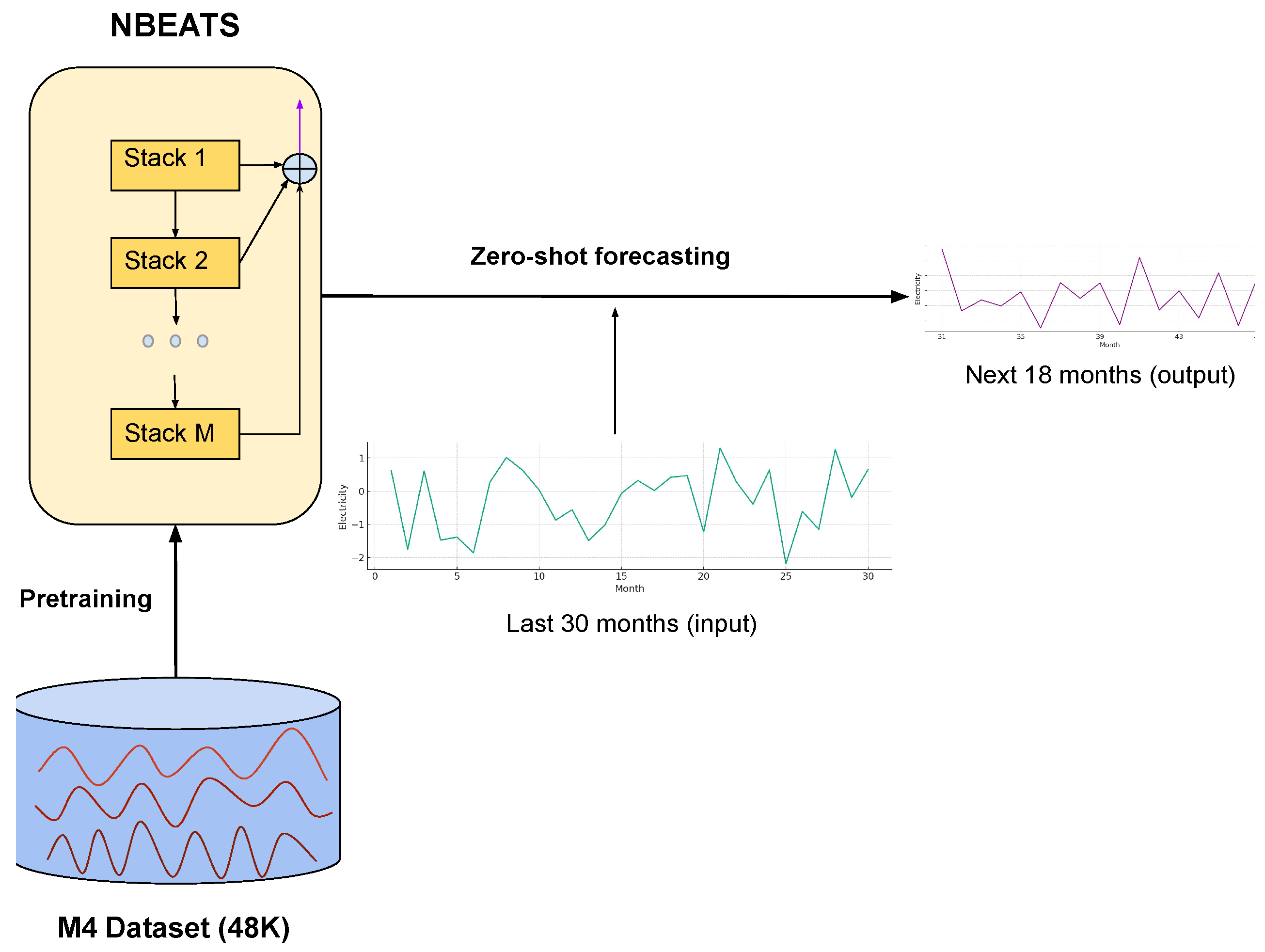
The proposed framework is illustrated in Figure 2. The NBEATS model is pretrained on a large dataset consisting of 48K monthly time-series obtained from a variety of domains. The pretrained model is used to perform forecasts directly on the unseen electricity input data. Unlike the traditional transfer learning paradigms, the proposed zero-shot approach does not require any additional fine-tuning of the pretrained model resulting in a more efficient forecasting model.

4. Experimental Results

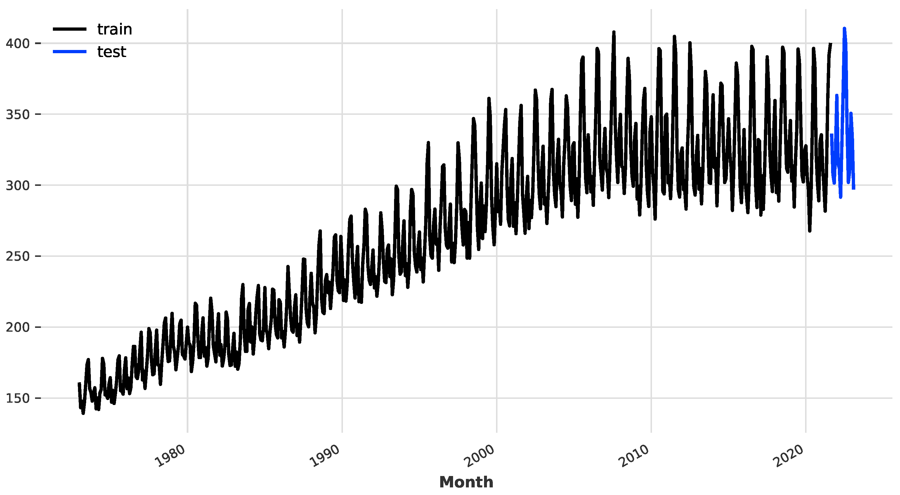
To evaluate the effectiveness of the proposed model, we compare it to several standard deep learning and statistical models. Specifically, we consider the RNN, GRU, LSTM, ARIMA, TCN, and XGBoost models. The dataset used for the experiment is the total monthly electricity production in the US from January 1973 to February 2023. As shown in Figure 3, the time series is split into training and testing sets, where the last 18 months are allocated as the testing set. The complete code for the numerical experiments is provided on GitHub at https://github.com/group-automorphism/zero-shot-energy-forecast.(accessed on January 12 2024).

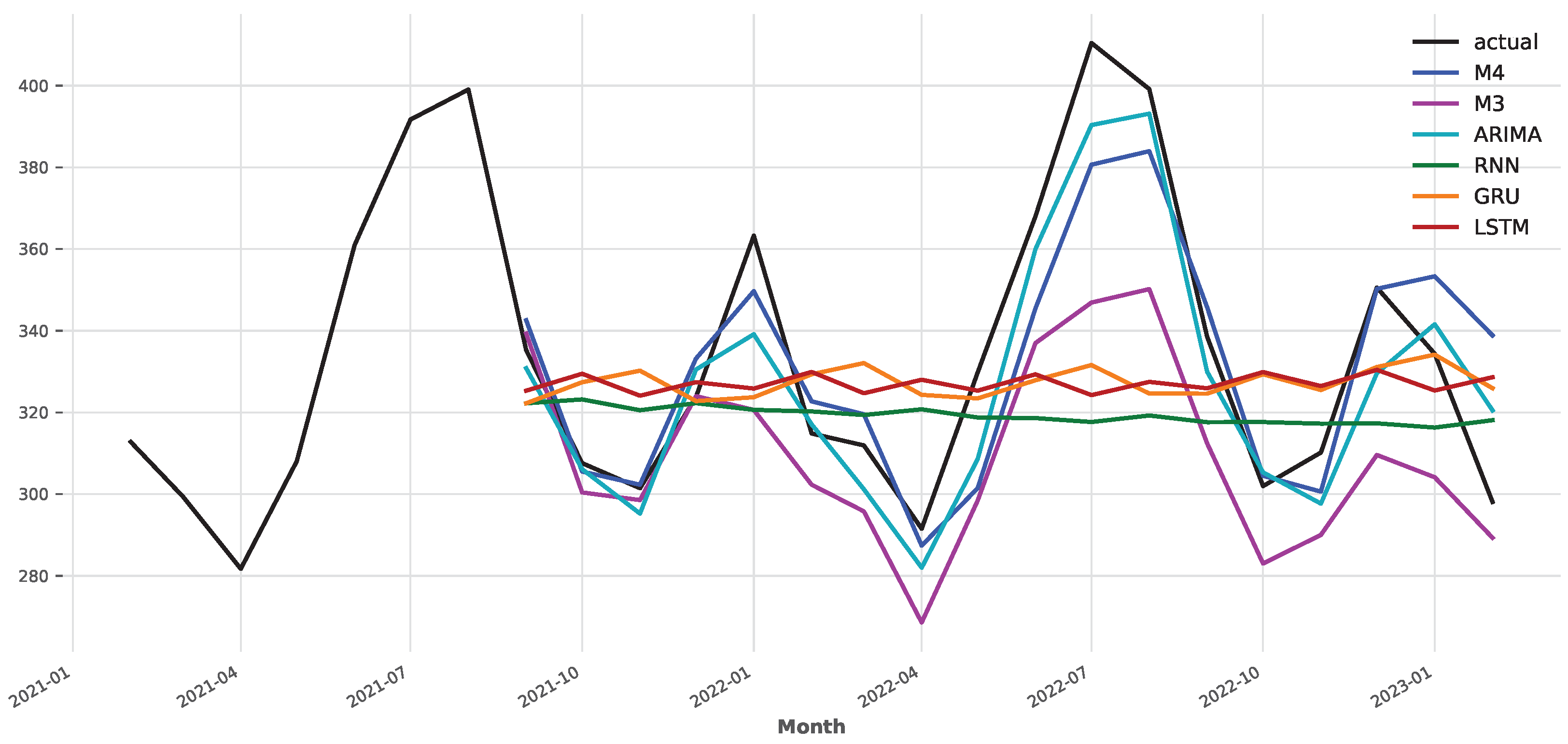
The forecasts of different models are presented in Figure 4. Note that the M3 and M4-based NBEATS models are not trained on the electricity training set and make forecasts directly using zero-shot learning. As shown in Figure 4, the NBEATS model is able to capture the downward spikes but struggles to predict the upward spikes in the time series. The M4-trained model significantly outperforms the M3-trained version. The mean absolute percentage error (MAPE) of the M4-based model is 3.742, while the M3-based model achieves MAPE = 7.573. In other words, pretraining on a larger dataset leads to higher forecast accuracy when using zero-shot learning. This is an unsurprising result as deep learning models often benefit from larger training data. It is also worth noting that MAPE = 3.742, achieved by the M4-based NBEATS model, is impressive given that it was trained directly on the electricity dataset. The results illustrate the effectiveness of transfer learning in electricity forecasting. It appears that the information learned from other time series can be successfully applied to new time series.

The benchmark models are evaluated according to the following scheme. Each model—RNN, GRU, LSTM, and ARIMA—is trained on the training set. The trained model is used to forecast electricity generation for the next 18 months. Note that, as with the NBEATS model, the deep learning models are trained with a 4-month forecast window and a lookback window of 30 months. Then, the 18-month forecast is performed recursively. The ARIMA model is trained using the number of lags $p=12$ and the order differentiation $d=1$. The forecast is compared with the test set values, and the MAPE is calculated.

As shown in Figure 4, both ARIMA and M4-trained models are able to trace the actual time series values with relative accuracy, while the traditional deep learning models—RNN, CNN, and LSTM—struggle to produce accurate forecasts.

Table 2. Accuracy metrics and execution times of the models in forecasting electricity generation 18 months ahead.

Model	MAPE	RMSE	Time
NBEATS_M4	3.742118	16.780905	0.151145
NBEATS_M3	7.572600	29.191671	0.196498
ARIMA	3.326473	13.099669	3.416353
RNN	8.396366	36.253910	9.510177
GRU	8.034973	33.665825	17.324589
LSTM	8.108890	34.101273	10.297812
TCN	5.053453	19.918373	14.026435
XGBoost	3.872260	14.467587	0.5724715

shows that ARIMA achieves the lowest error among all the tested models, with the M4-based NBEATS model running a close second. Since deep learning models usually contain a large number of parameters, they require a significant number of data for training. Since the training set in our electricity dataset was relatively small, the deep learning models overfit the data, which led to poor generalization on the test set. On the other hand, ARIMA is a parametric model and does not require a large dataset to estimate its model coefficients. Therefore, the results are in line with the theoretical expectations regarding the performance of the models. Importantly, the M4-based NBEATS model outperformed the deep learning benchmark models despite not being trained on the electricity data. This demonstrates the effectiveness of the proposed method.

The comparison of the execution times shows that the two NBEATS models are significantly faster than the benchmark models (Table 2). In particular, the M4-based model is more than 20× faster than ARIMA and nearly 70× faster than LSTM. The results illustrate the effectiveness of the zero-shot learning approach in reducing computing times while providing relatively accurate forecasts.

To obtain a better glimpse of the model performance, we evaluate each model using a 4-month forecasting horizon over the last 18 months of the test set. In other words, we backtest the models starting from the end of the training set’s period. In the case of ARIMA, we repeatedly build a training set expanding from the beginning of the series. The model is trained on the training set and a forecast is made, and the MAPE is evaluated on the forecast and the actual values. Then, the end of the training set is moved forward by 1 time step. Thus, in the first iteration, the training period for ARIMA is $[0,n_{tr}]$, while in the next iteration, the training period is $[0,n_{tr}+1]$, where $n_{tr}$ is the number of periods in the original training set. Finally, the mean of all the MAPE scores is calculated. In the case of RNN and other deep learning models, including NBEATS, the model is not retrained at each iteration; i.e., we employ the same model as trained on the original train set. Instead, only the lookback window is moved by one time step. Thus, in the first iteration, the lookback window is $[n_{tr}-30,n_{tr}]$, while in the next iteration, the lookback window is $[n_{tr}-29,n_{tr}+1]$.

As shown in

Table 3. The backtest error of the models in forecasting electricity generation.

Model	MAPE
NBEATS (M4)	5.387
NBEATS (M3)	7.005
ARIMA	5.468
RNN	5.565
GRU	12.028
LSTM	13.427
TCN	8.413305
XGBoost	6.966104

, the M4-based NBEATS model achieves the lowest backtest error. It outperforms both the deep learning and statistical approaches. Since the backtest is based on multiple forecasts—in this case, we made 14 test forecasts—it represents a more extensive evaluation of the model performance, which reveals the superiority of our proposed approach. As the NBEATS model was originally pretrained using a 4-month forecasting horizon, the results of the backtest indicate that in order to achieve optimal performance, the forecasting window used for future predictions should match the forecasting window used during the model training. Consequently, given a desired forecasting horizon, it is best to pretrain the NBEATS model using the same length horizon. On the other hand, as demonstrated in Table 2, the proposed approach works well even when the required forecasting horizon is longer than the one used during the training.

The results presented in Table 2 and Table 3 indicate that the proposed approach has significant potential. First, the M4-based NBEATS achieves the lowest error among all the tested models. Second, the comparison of the performance between the M3 and M4-based models shows that an increase in the training set size reduces the model’s error. Thus, we can further improve the performance of the proposed approach by pretraining on a larger dataset. Finally, since we employ zero-shot learning, the proposed method does not require additional training on new data, which provides a faster execution time. Indeed, the speed of the forecasting is arguably the greatest advantage of the proposed approach.

Since monthly data are relatively scarce—in our case, there are 600 months in 50 years—it is usually not enough to train deep learning models. Transfer learning is a useful tool when dealing with limited data. The results demonstrate that by pretraining on a large dataset—in our case, the M4 data contain around 48,000 different series—the model is able to learn the patterns inside the time series and generalize to unseen data. On the other hand, the traditional deep learning models trained on a single series with 600 time steps do not perform well.

Sensitivity analysis involves assessing how changes in input parameters influence the outcomes of a model. This process is crucial for pinpointing areas that may be vulnerable or require enhancement, as it helps in understanding the robustness and reliability of the model under varying conditions. In particular, we considered different lookback window lengths in training the base model. The lookback window length is a key model parameter and as such plays a critical role in the performance of the model. As shown in

Table 4. Sensitivity analysis of the lookback window length parameter in the M4-based NBEATS model.

Lookback	MAPE	RMSE	Time	Backtest
8	8.583	39.062	0.163	11.441
12	5.088	19.716	0.403	6.480
20	2.473	10.394	0.219	4.895
30	3.742	16.781	0.151	5.387

, the lookback period affects both the accuracy and execution time of the M4-based NBEATS model. We observe that a longer lookback period generally corresponds to higher accuracy. The effect on the execution time is mixed. Overall, based on the combination of speed and accuracy, lookback periods 20 and 30 provide the best performance.

5. Conclusions

In this paper, we proposed a novel approach to forecasting electricity generation using zero-shot learning. Specifically, an NBEATS model pretrained on a large corpus of time series data was used directly, without any additional training, to predict the quantity of generated electricity. The results indicate that the proposed approach has significant potential. The M4-based NBEATS model outperformed all the standard deep learning forecasting models. In addition, it outperformed ARIMA in the backtest. Since the proposed method uses zero-shot learning, it provides faster execution time than the models that require data-specific training.

The difference between the performance of the M3- and M4-based models indicates that the proposed approach can be further enhanced by employing a larger dataset in pretraining. Thus, the exploration of forecasting models based on larger pretraining datasets using transfer learning presents an interesting avenue for future research. Since one of the main advantages of the proposed method is the speed of execution, it would be particularly useful in the context of high-speed forecasting such as high-frequency energy trading platforms. Therefore, the application of the proposed method in high-speed forecasting environments is another avenue for future research.

The main drawback of the proposed approach is the initial pretraining, which requires considerable time and resources, as well as a large and diverse dataset. In the absence of the required resources the proposed approach is likely to underperform compared to the more traditional parametric methods such as ARIMA, which thrive in constrained data environments.