Comparison of Empty and Oil-Filled Transformer Tank Mode Shapes Using Experimental and FEM Modal Analysis

Abstract

In this paper, the mode shapes of an empty and oil-filled transformer experimental model tank are obtained using 3D finite element method (FEM) modal analysis. For verification of the FEM analysis results, experimental modal analysis (EMA) is carried out in both cases using appropriate impact hammers and accelerometers. Simulated and measured results are visualized and compared for mode shapes in a frequency range of interest for both empty and oil-filled tanks. In order to avoid overly stiff FEM models of transformer tanks, the welded joint modeling technique is presented and analyzed in detail. For an oil-filled tank, the most accurate results are calculated in the model where the welded joint is modeled as half the tank wall’s thickness. In that case, the mean absolute error for the given ten-mode shapes is 1.7 Hz. Also, mesh sensitivity analysis is performed. It is concluded that a 10 mm maximum element size is an optimal solid (3D) mesh. However, shell mesh can be used to reduce computing requirements.

1. Introduction

Experimental modal analysis (EMA) is primarily used for detecting structure resonance and mode shapes. If transformer tank resonance occurs, load noise can be increased by 8–10 dB [1]. There is no similar data for no-load noise, but it should be in the same range. The important application of the EMA is verifying mechanical finite element method (FEM) analysis. Validation of a FEM modal analysis of a transformer tank with the EMA is presented in the literature [2,3,4,5]. In some research papers, that step is skipped, and only the vibrations of the tank in operation are measured and compared with FEM [6].

Furthermore, the FEM modal analysis can be used to compare the resonances of the different tank design solutions [7]. A similar approach can also be applied to various machines, such as turbine rotors [8]. A flow-optimized turbine rotor shape is redesigned to avoid resonant frequencies. The dynamic characteristics of an oil-filled transformer can be calculated using FEM modal analysis to predict the part of the transformer that radiates the most noise [9] or to see the influence of tank design parameters such as thickness on the resonant frequencies [10]. The oil inside the tank adds mass to the structure and changes its vibration response. Therefore, comparing the FEM analysis of an empty tank with the EMA can provide validation of the FEM model of the tank. On the other hand, comparing the oil-filled tank to the EMA can provide verification of the modeling of fluid–structure interaction (FSI). In the literature, several approaches to FSI modeling of water-filled tanks can be found [11,12,13]. There is also an example of FEM modal analysis of an elevated water tank with various water levels and an empty tank [14]. FSI is modeled using two approaches. The first is a simplified approach with a spring-mass system and the second is an approach with acoustic solid elements. EMA can also be used for the validation of other techniques for modes and natural frequency extraction, such as operational modal analysis [15]. There is also an approach in the literature where tank resonances are calculated analytically to avoid computationally expensive FEM calculations [16].

Frequency response functions (FRF) used to determine resonant frequencies and mode shapes can also be measured from the active part to an empty and oil-filled tank. The purpose is to determine where most energy is transferred through oil or structure [17,18].

The motivation for the work is to validate a FEM model for calculating radiated transformer noise in several steps. The first steps presented in this paper are validation of the FEM model of the empty tank using EMA and validation of fluid–structure interaction (FSI) modeling by comparing the FEM model of an oil-filled tank with EMA. There are several challenges in EMA. Linearity should be satisfied, and signal processing errors should be avoided. In FEM analysis, challenges include adequate welded joint modeling, contact definition, mesh size, etc. Compared to previous research that considered transformer tank modeling [2,3,4,6,7,9,10], this study fills the gap in a welded joint modeling methodology for FEM models of the transformer tanks. As the tank is an emitter of the sound coming from the active part, adequate tank modeling in FEM is a crucial step in the accurate numerical calculation of radiated noise.

In this work, a brief overview of EMA and FEM modal analysis theory is presented. The methodology of EMA for the tank of the transformer experimental model is presented, and FEM models of an empty tank and an oil-filled tank are calculated. The FEM analysis is validated with the presented EMA analysis, and mode shapes on the tank are shown. At the end, a discussion and conclusion are given, along with a comprehensive overview of the contributions, possible applications of the findings, a summary of the results, and future work that needs to be done.

2. Theoretical Considerations

In this paragraph, basic mathematical expressions that describe EMA and equations used in FEM modal analysis are given.

2.1. Experimental Modal Analysis (EMA)

The structure tested by EMA is assumed to be linear, time-invariant, and must obey Maxwell’s reciprocity theorem [19]. The basic principle of EMA is finding a ratio between measured excitation at one location and applied force at another location as a function of frequency. That ratio is a complex mathematical function called the frequency response function (FRF). A mathematical representation of a single-input relationship is given as:

$$\left[\begin{array}{c}{X}_1\\ X_2\\ \begin{array}{c}·\\ ·\\ X_p\end{array}\end{array}\right]=\left[\begin{array}{c}{H}_{1q}\\ H_{2q}\\ \begin{array}{c}.\\ .\\ H_{pq}\end{array}\end{array}\right]F_q$$

(1)

where X_p is a response in point p, F_q is excitation in point q, and H_pq is an FRF between points p and q.

If the linearity of modal analysis is satisfied, then the system’s response can be obtained as a combination of specific modes. The linearity can be checked by comparing the amplitude and resonant frequencies of FRF when changing the excitation amplitudes [20]. The reciprocity property states that a force applied at degree of freedom (DOF) p that results in a response at DOF q is the same as the response at DOF p caused by the same force at DOF q. That can be checked by selecting the two points on the structure and changing the excitation (hammer) and response (accelerometer) points. That can be expressed as:

$$H_{pq}=\frac{X_p}{F_q}=H_{qp}=\frac{X_q}{F_p}$$

(2)

Boundary conditions of the structure can be either free-free or fixed. Also, attention should be paid to signal processing errors and solutions, such as aliasing, leakage, windowing, filtering, zooming, and averaging [21].

2.2. FEM Modal Analysis

The governing equation of an un-damped free harmonic vibration is:

$$\left[-{\omega }_i^2\left[M\right]+\left[K\right]\right]\left\{{\mathsf{\Phi }}_i\right\}=\left\{0\right\}$$

(3)

where [M] and [K] are mass and stiffness matrices, respectively, ω_i is the ith natural frequency, and {Φ_i} is a displacement amplitude that represents the mode shape corresponding to ω_i. Equation (3) represents a typical eigenvalue problem, and a nontrivial solution to that is:

$$\det \left(-{\omega }_i^2\left[M\right]+\left[K\right]\right)=0$$

(4)

The natural frequency is calculated from Equation (4). After importing the results in (3), mode shapes can be calculated. Solving fluid–solid interaction problems, except Newton’s equation of motion for solids, involves solving the Navier–Stokes equations for the fluid. Since the continuity equation can be used in multiple physical phenomena, such as in the analysis of the velocity of carriers in a high-field region [22], it can also be applied in fluid dynamics. Continuity requires that the normal component of particle velocity ∂Ψ/∂n of the fluid equal the normal component of the surface velocity v_n of the solid at the interface, as is written with the following equation:

$$v_n=n·\left(\frac{\partial u}{\partial t}\right)=-n\nabla \psi =-\frac{\partial \psi }{\partial n}$$

(5)

where u is the displacement vector.

3. Materials and Methods

This paragraph gives the methodology of EMA, including measurement procedure, measurement equipment, and environmental controls. Also, FEM modal analysis setup with a step-by-step process and FEM parameters are described in detail.

3.1. EMA on the Transformer Tank

The EMA measurements on the transformer tank are carried out using SIMO (single-input, multiple-output) analysis. In other words, hammer excitation force is always applied at the same point, and acceleration is measured at all 164 points on the tank surface of the transformer experimental model. The model’s tank dimensions are 1.16 m in length, 0.47 m in width, and 1.31 m in height from the tank bottom to the tank cover. The tank is constructed without a conservator or stiffeners. A latter is decided in order to simplify the calculations, especially for future research when the core and the windings will be considered. Before measurements, it is necessary to check the linearity and reciprocity. The verification is made for two hammer types and various hammer tips.

After selecting an appropriate impact tool, the EMA of the transformer experimental model tank is carried out for the empty and oil-filled tank cases. A specification comparison of two impact hammers used for the measurements is given in

Table 1. Specifications comparison of two types of impact hammers and the accelerometers used for the measurements.

Impact Hammer	PCB 086D20	KISTLER 9724A2000	Accelerometer	PCB Piezoelectronics 608A11
Sensitivity [mV/N]	(±15%) 0.23	2	Sensitivity (±15%) [mV/(m/s2)]	10.2
Measurement range [N pk]	±22,240	±2000	Measurement range [m/s2]	±490
Hammer mass [kg]	1.1	0.25	Enclosure Rating	IP68

. The response of the system is measured by three accelerometers, PCB Piezoelectronics 608A11 (Table 1). The Dewesoft data acquisition system, hardware and software, is used to measure and store the results. A Wheater station data logger, the Trotec DL200D, is used to check the environmental conditions during the measurements. The temperature ranged from 29 °C to 33 °C, relative humidity from 60% to 70%, and atmospheric pressure between 1000 and 1020 hPa. The tank is mounted on a stable wooden base with no additional vibration insulation pads added at the bottom. The ambient noise that could influence the measurements is not measured, but the experiments are done in conditions with minimum noise. A calibration certificate from the impact hammer manufacturer is used to enter the sensitivity value. An additional calibration in an accredited laboratory is done for the accelerometers to get the sensitivity in the range of frequencies from 10 to 1000 Hz. Also, before each measurement set, a calibrator of B&K type 4294 is used to check sensitivity at 159.15 Hz. Finally, MATLAB is used to process the measurement results and visualize mode shapes.

The measurement equipment used for the EMA and the test object are shown in Figure 1a. The moment of EMA measurement on the tank is shown in Figure 1b. The excitation is measured at one point and the response at three points simultaneously. The same procedure is used on both empty and oil-filled tanks.

3.2. FEM Modal Analysis of Empty and Oil-Filled Tank

The flowchart of a detailed step-by-step diagram of tank modeling and validation methodology from this research (part in the red rectangle) that has a final goal of a validated FEM vibroacoustic model of a transformer is shown in Figure 2.

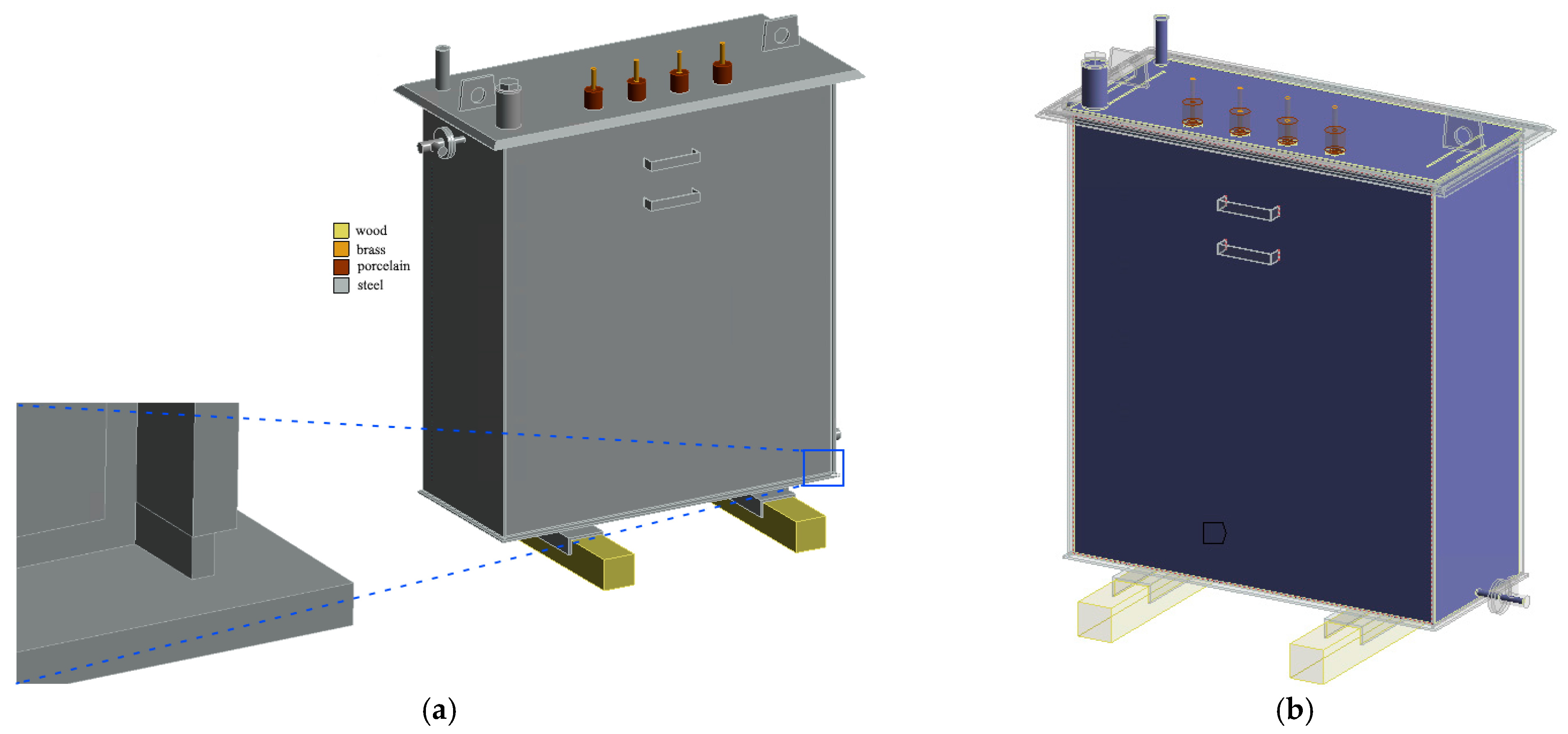
In order to mesh and solve the FEM model correctly, geometry simplifications on the CAD model need to be made. The simplified geometry of the transformer tank used for FEM analysis is shown in Figure 3a. Considering the materials in the model, except the structural steel as the tank material, brass (leads), porcelain (insulators), and wood (base) are used. Structural steel influences the system’s response most, so Young’s modulus is measured for an S235 steel grade of 6 mm thickness used to construct the tank. It is measured on the 10 specimens by applying tensile stress. Five specimens are obtained by cutting in a longitudinal direction, and five specimens by cutting in a transversal direction. The given mean value of Young’s modulus is 187.1 GPa, with a standard deviation s equal to 7.8 GPa. In the FEM analysis, Young’s modulus is set to 190 GPa. The properties of all the materials mentioned in the analysis are given in

Table 2. Properties of materials used in modal FEM simulations.

Material	Steel	Brass	Porcelain	Wood
Density [kg/m3]	7850	8670	2300	1100
Young modulus [GPa]	190	127	67	8
Poisson’s ratio	0.3	0.32	0.17	0.3

.

A fixed support boundary condition is set at the bottom of the wooden base. In the fixed support boundary condition, the structure is prevented from any translational and rotational movement. Bonded contacts are avoided in FEM models in the sense that a shared topology feature is used. Application of that feature imprints and merges all bodies into components, considered multi-body parts. Also, a conformal mesh is created, which means that parts share nodes at the interface, which leads to more accurate results.

Oil in the model is added as an acoustic region with a density of 866 kg/m³ and a speed of sound of 1390 m/s. All the other bodies are defined as structural regions. Fluid-structure interaction is set on the oil faces inside the tank. Air is not considered because acoustic calculations are not in the scope of this work. The FSI on the surfaces of the oil is shown in Figure 3b. Both empty and oil-filled tank models are meshed with a maximum element size of 10 mm. The empty tank model consists of 532,649 nodes and 189,143 elements, and the oil-filled tank model consists of 735,790 nodes and 364,680 elements. In Section 4.5, mesh sensitivity analysis is performed, and the mesh size selection is explained in more detail. In the FEM modal analysis, it is not necessary to give an excitation because, as shown in (3), only mass and stiffness matrices are necessary to calculate the resonant frequencies and associated mode shapes.

Experience showed that modeling the welded joints as bonded contacts in FEM results in overly stiff models, and resonant frequencies are too high compared to the measurements. In order to avoid that problem, the welded joint is modeled as a frame, and its thickness is gradually decreased, as shown in the diagram in Figure 2. The optimal solution is achieved when modeled as a 3 mm frame, half the tank wall’s thickness, as shown in Figure 3a. In Section 4.4., the influence of welded joint modeling on the resonant frequencies is analyzed and explained in more detail.

4. Results

In this paragraph, the results of linearity and reciprocity of EMA using two different impact hammers for the empty and oil-filled tanks are carried out. Also, a comparison of the EMA mode shapes of the empty and oil-filled tanks with FEM analysis results for specific resonant frequencies is shown. In the end, the influence of welded joint modeling and mesh sensitivity analysis are performed, and the mean absolute error is calculated to compare the results quantitatively.

4.1. Linearity and Reciprocity of EMA

Linearity is necessary for the system to be suitable for modal analysis. As mentioned, it is assumed that combining certain modes can produce the system’s response. The reciprocity relationship holds only for linear and time-invariant systems. It allows more efficient testing, so conducting a separate test for each excitation and response point is unnecessary. In that case, a SIMO analysis can be carried out.

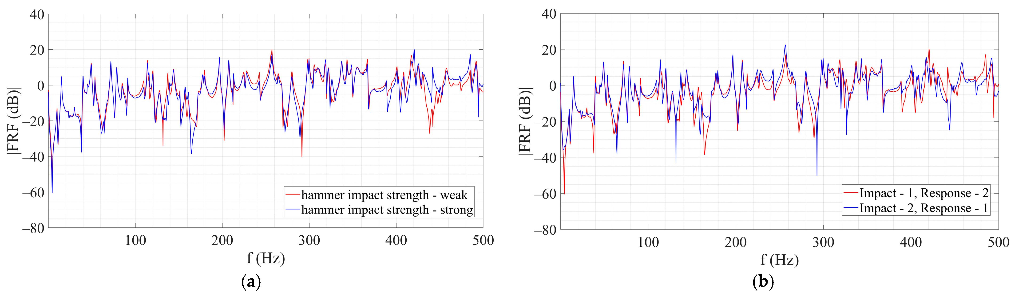
Linearity and reciprocity verification using PCB (larger) and KISTLER (smaller) impact hammers on an empty tank are shown in Figure 4 and Figure 5, respectively. The hardest tip is used for the PCB impact hammer to excite a more extensive range of frequencies. The tip of medium hardness is chosen for the KISTLER impact hammer because the range of frequencies above 1000 Hz is unimportant for transformers. Theoretically, both FRF curves on each graph should be the same. Impact strength and the replacement of points at which impact and response are measured should not influence the FRF. Verification shows the analysis is linear and reciprocal, especially from the 0 to 400 Hz range and for the PCB impact hammer.

Linearity and reciprocity verification using a PCB impact hammer on the oil-filled tank is shown in Figure 6. According to the verification results, FRF functions are even more similar than in the test without the oil. Linearity and reciprocity of the analysis are confirmed, and EMA can be carried out.

4.2. Comparison of EMA and FEM Analysis of an Empty Tank

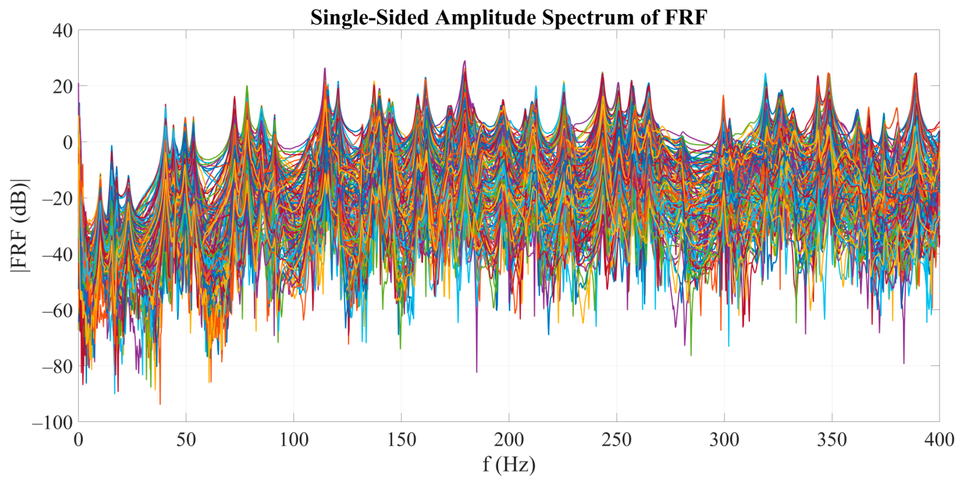
All 164 single-sided amplitude spectrums of FRF functions in dB from the EMA of the empty tank are shown in Figure 7. Resonant frequencies are visible as the peaks of the FRFs, and it is evident that they match in all measurements.

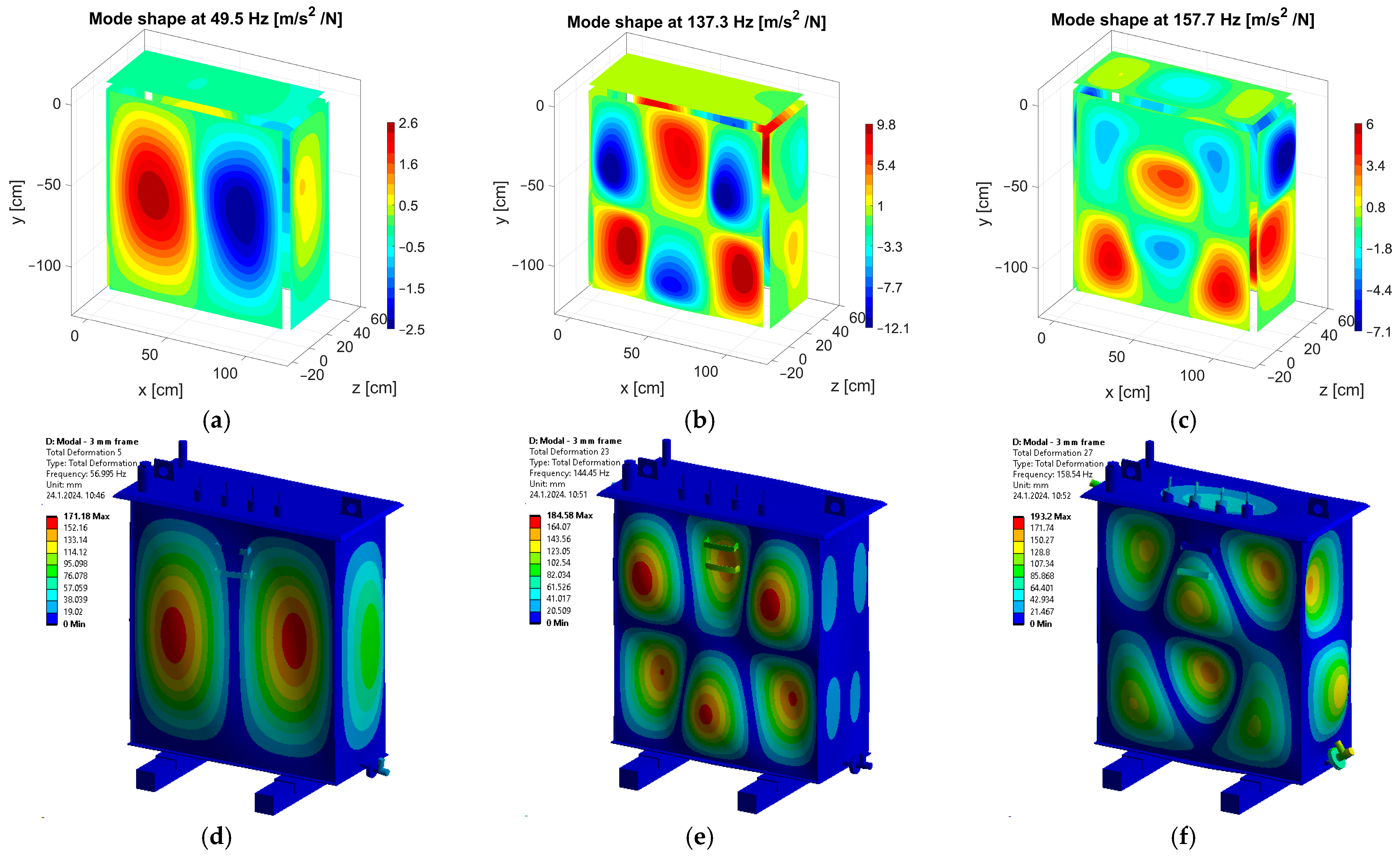
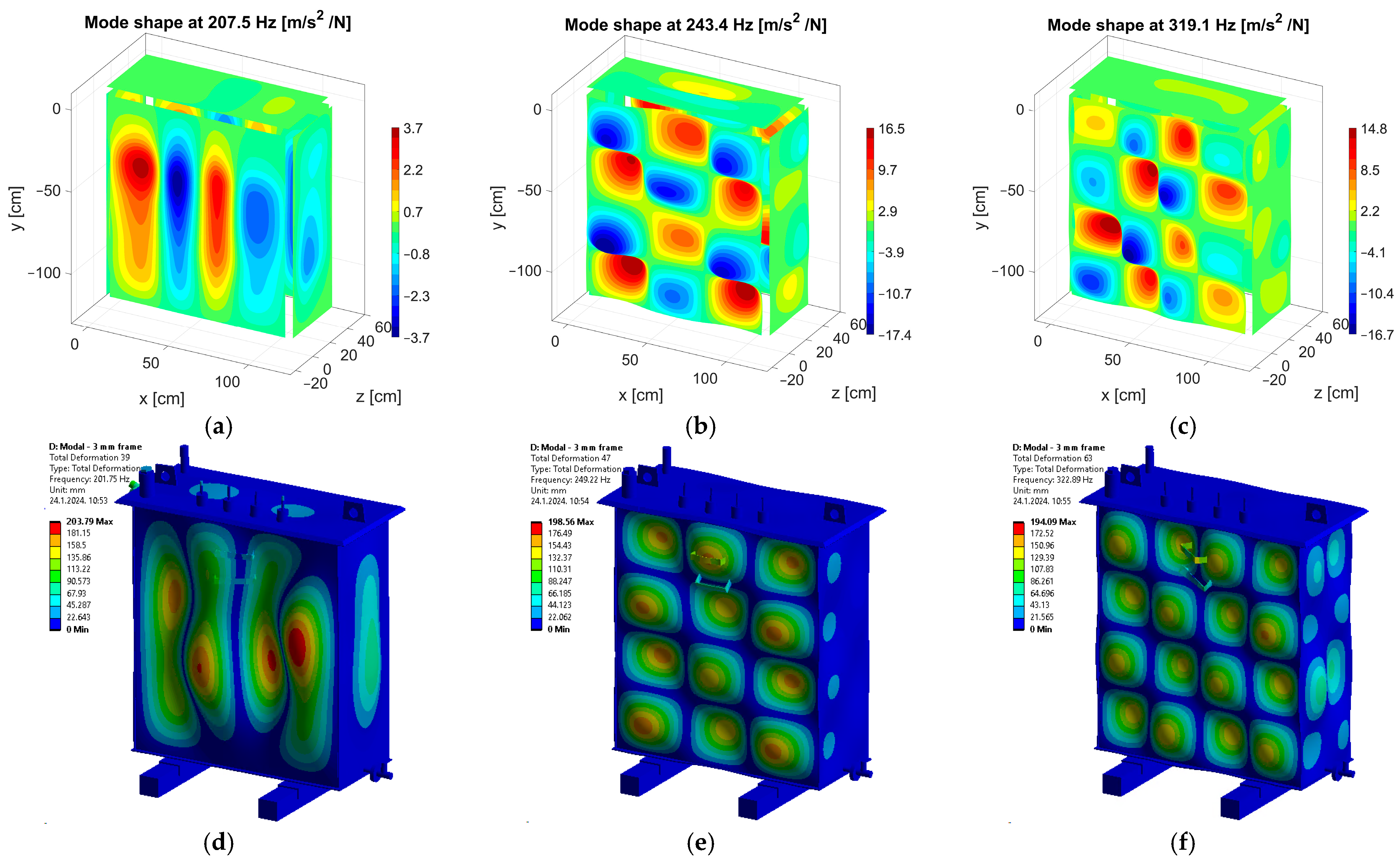
The six simulated and the same six measured mode shapes of an empty tank are shown in Figure 8 and Figure 9. FEM modal analysis results have higher resonant frequencies than EMA results. It varies from shape to shape but can be up to 20 Hz, as in the case of the mode shape (3,2) measured at 114.5 Hz and simulated at 134.2 Hz. A more detailed analysis of welded joint modeling is given in paragraph 4.4. Optimization of the simulated value can be obtained by decreasing the thickness of the frame to 1 mm. Then, the simulated mode shape (3,2) has a resonant frequency of 116.2 Hz, as shown in

Table 3. Comparison of resonant frequencies of specific mode shapes for different welded joint modeling techniques (no frame, 3 mm frame, and 1 mm frame) with EMA for the empty and oil-filled tank with calculated EMA.

Mode Shape	Empty Tank Resonant Frequencies [Hz]				Oil-Filled Tank Resonant Frequencies [Hz]
	EMA	No Frame	3 mm Frame	1 mm Frame	EMA	No Frame	3 mm Frame	1 mm Frame
(2,1)	40.5	56.8	55.1	46.2	17.1	19.7	18.0	13.7
(1,2)	49.5	58.3	57.0	52.8	27.4	33.4	31.5	26.0
(2,2)	72.5	89.7	85.7	78.6	43.8	50.9	47.7	40.8
(3,2)	114.5	141.7	134.2	116.2	67.9	74.0	68.4	56.9
(2,3)	137.3	150.0	144.5	133.0	77.4	80.2	77.5	73.0
(4,1)	145.9	167.9	161.6	148.1	91.2	93.3	91.2	87.5
(3,3)	196.1	196.7	188.9	176.7	112.4	121.2	116.6	106.5
(2,4)	212.5	221.3	216.7	207.2	134.4	139.4	134.7	122.3
(4,3)	243.4	260.3	249.2	235.6	157.1	164.9	156.7	142.4
(4,4)	319.1	333.4	322.9	310.2	215.3	219.5	212.8	196.2
	MAE	14.5	9.9	6.5	MAE	5.3	1.7	7.9
	s	7.4	5.5	5.1	s	2.3	1.8	6.0
	range	0.6–27.2	3.8–19.7	1.7–19.4	range	2.1–8.8	0–4.2	1.4–19.1

. An example of a mode shape where the simulated frequency is lower than measured is shown in Figure 9a,d.

4.3. Comparison of EMA and FEM Analysis of Oil-Filled Tank

All 164 single-sided amplitude spectrums of FRF functions in dB from the EMA of the oil-filled tank are shown in Figure 10. Resonant frequencies match in all the measurements, and modal density is higher than for the empty tank, especially in the range of up to 100 Hz.

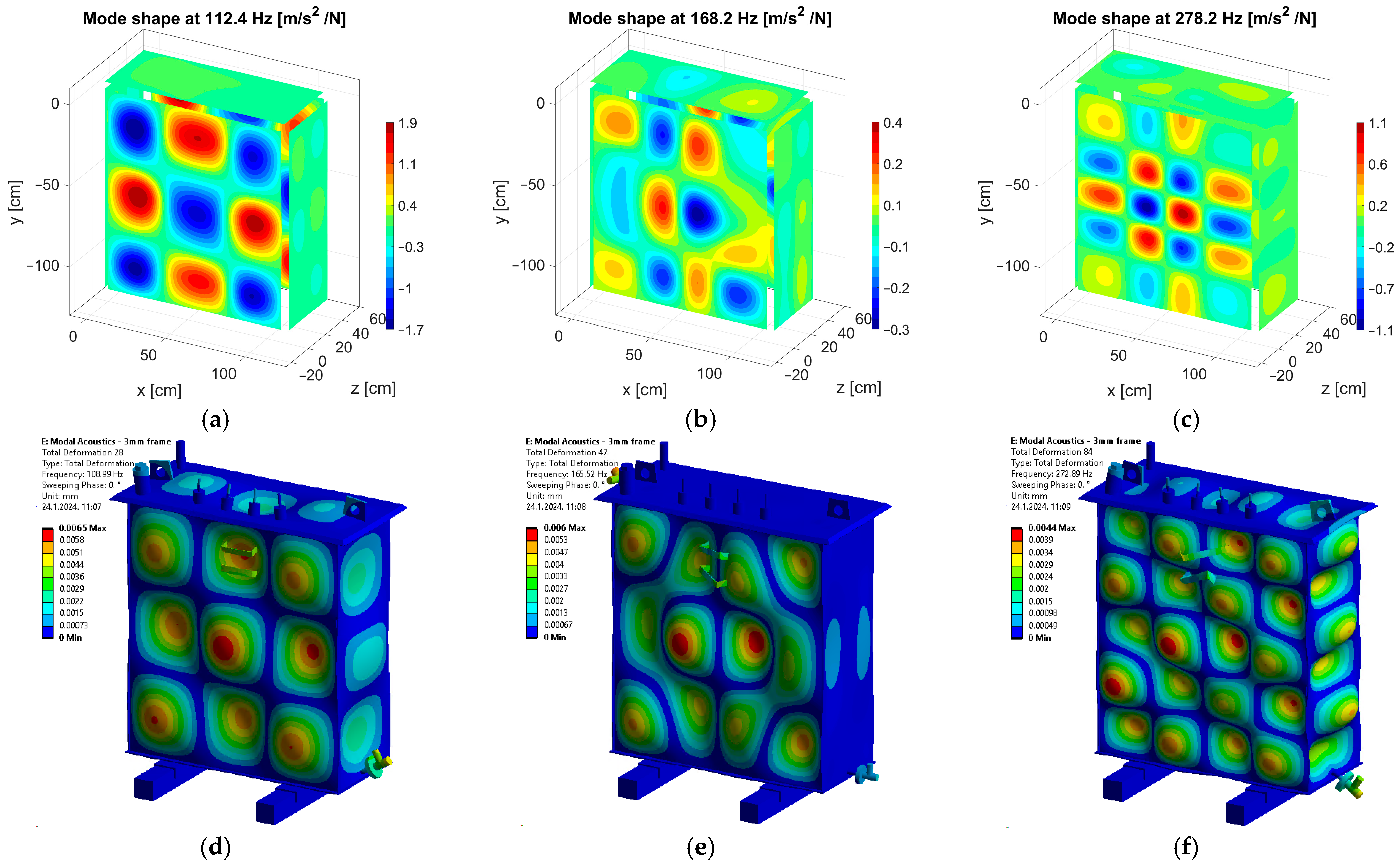
The six simulated and the same six measured mode shapes of an oil-filled tank are shown in Figure 11 and Figure 12. Differences between simulated and measured resonant frequencies for the same mode shape are lower than in the case of the empty tank. Although matching between simulated and measured mode shapes on the front tank wall side is good, mode shapes on the lateral side and the tank cover are not always the same. Examples are the mode shapes in Figure 11a and Figure 12a. There are also cases where there is a perfect match at each transformer tank surface, as for the mode in Figure 11c.

4.4. Influence of Welded Joint Modeling on the Resonant Frequencies

Resonant frequencies of specific mode shapes for different welded joint modeling techniques compared with EMA for empty and oil-filled tanks are shown in Table 3. The first technique is without a frame (standard connection), the second is 3 mm, and the third is a 1 mm frame. Modeling thinner frames results in lower resonant frequencies in empty and oil-filled models. The mean absolute error (MAE) is calculated for ten modes from Table 3. The MAE is defined as:

$$\mathrm{M}\mathrm{A}\mathrm{E}=\frac{1}{n}\sum _{i=1}^{10}\left|f_{FE{M}_i}-f_{EM{A}_i}\right|$$

(6)

where f_FEMi is the FEM calculated resonant frequency of the ith mode shape, and f_EMAi is the measured EMA resonant frequency of the ith mode shape. Except for the MAE, statistical parameters such as standard deviation (s) and range are also added to provide more detailed information about the distribution of the data set.

A frame of 1 mm thickness provides the most similar resonant frequencies compared to the EMA measurements for the case of an empty tank. In that case, the MAE is the smallest (6.5 Hz). In the case of an oil-filled tank, MAE is the largest for a 1 mm thickness. The best results are calculated using a selected 3 mm frame. In that case, the MAE for the given ten-mode shapes is 1.7 Hz. It is also visible that resonant frequencies for a selected 3 mm frame are, on average, 8.4 Hz higher in FEM models of an empty tank and 1.1 Hz higher in FEM models of an oil-filled tank than in EMA.

4.5. Mesh Sensitivity Analysis

Tanks in all the models used in this paper are meshed with a 10 mm maximum element size. Mesh sensitivity analysis is performed with four additional FEM models for the case of the empty tank with a 3 mm frame. Those are 50 mm, 20 mm, and 5 mm maximum element size solid models, and a model with a shell mesh with a maximum element size set to 5 mm. An additional shell mesh model with no frame is added for comparison.

In the case of shell mesh models, valves and bushings with leads are not modeled. The rest of the parts are modeled as midsurfaces with a specified thickness. A shared topology feature, as in solid (3D) mesh models, is used where applicable. For the rest of the parts, bonded contact is used. For bonded contact, no sliding or separation is allowed. In a model with no frame, bonded contacts are between steel bars and the bottom of the tank and between a flange and a tank cover. For a model with a 3 mm frame, except for those parts, it is also between the frame and the tank wall. The definition of bonded contacts in both shell mesh models is shown in Figure 13.

Comparison of resonant frequencies at specific mode shapes of five FEM models for the case of an empty tank with a 3 mm frame for different maximum element sizes, a shell mesh model for that case, and a shell mesh model for a case of an empty tank with no frame is shown in

Table 4. Comparison of resonant frequencies of specific mode shapes for a model of an empty tank with a 3 mm frame for different maximum element sizes of a mesh and two shell mesh models.

Mode Shape	EMA	50 mm	20 mm	10 mm	5 mm	Shell Mesh (5 mm)	Shell Mesh No Frame (5 mm)
(2,1)	40.5	57.9	55.5	55.1	54.9	53.8	58.9
(1,2)	49.5	58.2	57.1	57.0	56.9	56.5	59.4
(2,2)	72.5	88.3	86.0	85.7	85.4	84.7	90.6
(3,2)	114.5	143.4	134.8	134.2	133.7	131.5	142.7
(2,3)	137.3	153.9	145.1	144.5	144.0	143.4	152.7
(4,1)	145.9	177.3	162.6	161.6	160.8	161.6	171.6
(3,3)	196.1	209.1	189.7	188.9	188.3	185.6	198.9
(2,4)	212.5	252.0	217.4	216.7	216.1	214.5	225.3
(4,3)	243.4	292.7	250.0	249.2	248.4	245.1	262.3
(4,4)	319.1	379.6	324.0	322.9	321.8	321.6	335.0
	MAE	28.1	10.4	9.9	9.5	8.8	16.6
	s	17.1	5.5	5.5	5.5	5.7	7.3
	range	8.7–60.5	4.9–20.3	3.8–19.7	2.7–19.2	1.7–17	2.8–28.2

. It is visible that reducing the mesh size reduces the MAE. For a 5 mm case, two elements per tank thickness (6 mm) are obtained. That case decreases the MAE for 0.4 Hz compared to a 10 mm case used in the model. The smallest MAE is obtained for a shell mesh case, 1.1 Hz smaller than the 10 mm mesh model.

On the other hand, shell mesh application for a model with no frame increased the MAE by 2.1 Hz compared to the same 10 mm mesh model in Table 3. It can be concluded that a 10 mm model is correctly selected as an optimal solid (3D) mesh model. Nevertheless, shell mesh models are recommended to reduce the computing requirements, even though some parts will be omitted from the model.

5. Discussion

A validation of FEM models is done using EMA for both empty and oil-filled tanks. The comparison of FEM and EMA showed that modeling the welded joints as bonded contacts in FEM results in overly stiff models. That is more emphasized in the case of an empty tank. This research proposes a modeling approach for a welded joint as a frame of reduced thickness to lower resonant frequencies. However, precautions should be taken in selecting the frame’s thickness. For example, in the case of modeling a frame of 1 mm thickness, the smallest error in calculated resonant frequencies is obtained for an empty tank model. In the case of the oil-filled tank, the error is largest for a 1 mm frame. The reason is that the FSI condition set on the structure changes its response, and the model is not as stiff as in an empty tank case. Then, modeling a 1 mm frame results in resonant frequencies that are too low. It is also important to note that this simplified tank has no stiffeners that can change its response and oil influence even more.

None of the research conducted to date where transformer tank FEM simulations were used did not consider welded joint modeling problems in the context of modal, harmonic vibration, or acoustic analysis. That includes the research where stiffeners are considered [2,3,7] and even those where tanks without stiffeners, as is the case in this research, are taken into account [4,6,9,10]. The most important contribution and novelty that this work provides is that it considers and, in detail, analyzes the problem of welded joint modeling and proposes a developed methodology and solution for the given problem. Also, it uses visualization methodology from the previous work [23] to enable a simple comparison of transformers’ measured and calculated mode shapes.

This FEM modeling approach increases the accuracy of transformer tank resonance calculations and allows for more reliable tank geometry (shape and size) optimization and resonance avoidance. It can also be used for more sufficient checks of transformer seismic load withstand capability and to detect areas prone to fatigue. Also, as mentioned before, an accurate tank model is a mandatory precondition to predict the noise radiated to the environment.

6. Conclusions

In this paper, EMA measurements are carried out on the transformer experimental model’s tank using SIMO analysis. Acceleration is measured at 164 points on the tank wall and cover, and excitation force is applied at a single point on the tank. Measurements are made on an empty tank and an oil-filled tank. Linearity and reciprocity are confirmed in both cases before EMA measurements.

The FEM model is created, and welded joints are modeled as a 3 mm frame, which is half the tank wall’s thickness. Oil in the model is added as an acoustic region, and all the other bodies are defined as structural regions. Fluid-structure interaction is set on the faces of the oil inside the tank.

Resonant frequencies can be detected as the peaks of FRFs, and they match in all the measurements of both empty and oil-filled tanks.

Comparing the mode shapes in both cases, it is visible that FEM modal analysis gives higher resonant frequencies than experimental results. That is especially emphasized for an empty tank, for which simulation gives 8.4 Hz higher resonant frequencies. For an oil-filled tank, resonant frequencies are 1.1 Hz higher for selected 10 mode shapes.

The six simulated and the same six measured mode shapes of an empty and oil-filled tank are visualized on a transformer in 3D space and compared. The resonant frequencies of the oil-filled tank are lower than those of the empty tank. In some cases, where the matching between simulated and measured mode shapes on the front tank wall side is good, the same mode shape is not obtained on the lateral side and the tank cover.

Modeling thinner frames results in lower resonant frequencies for the model. The best results are obtained for the 3 mm frame in the oil-filled tank model, and the mean absolute error (MAE) for the specific 10 mode shapes is 1.7 Hz.

Mesh sensitivity analysis showed that a 10 mm model is correctly selected as an optimal solid (3D) mesh model, but shell mesh models are recommended for future applications to reduce the computing requirements, especially for simpler tanks.

The presented methodology for validating transformer tank and oil (FSI) modeling is the first step in a chain whose aim is FEM modeling of transformer noise radiated to the environment. In the future, computational fluid dynamics (CFD) can be incorporated into the analysis to obtain even more accurate results. The main focus of future research will be validating the active part (core and windings) using EMA and vibroacoustic measurements. The first step will be a comparison of the FEM modal analysis of the core and windings with the associated EMA. After that, a coupled analysis in which magnetostrictive forces in the core and Lorentz forces in the windings will be imported as an excitation in harmonic mechanical analysis to calculate their vibrations. If acoustical region and FSI are used, vibrations on the tank and radiated sound pressure levels can also be calculated and compared to measurements.

References

- Girgis, R.S.; Bernesjö, M.; Anger, J. Comprehensive analysis of load noise of power transformers. In Proceedings of the 2009 IEEE Power and Energy Society General Meeting, PES ’09, Calgary, AB, Canada, 26–30 July 2009. [Google Scholar]
- Al-Abadi, A.; Gamil, A.; Schatzl, F. Detecting and Controlling Tank Resonance of Oil Immersed Power Transformers. In Proceedings of the DAGA 2018 Munchen, München, Germany, 19–22 March 2018. [Google Scholar]
- Ma, Y.; Wan, W.; Mo, J.; Li, X. Experimental Study on the Vibration Characteristics of Oil Tank Model of Oil-Immersed Transformer. IOP Conf. Ser. Earth Environ. Sci. 2020, 508, 012211. [Google Scholar] [CrossRef]
- Wang, G.; Yao, D.; Ma, Y.; Zhang, S.; Wang, G.; Xu, L.; Wang, L. Test and Analysis of Vibration Mode of Distribution Transformer Tank Structure. IOP Conf. Ser. Earth Environ. Sci. 2020, 526, 012098. [Google Scholar] [CrossRef]
- Case, J. Numerical Analysis of the Vibration and Acoustic Characteristics of Large Power Transformers. Ph.D. Thesis, Queensland University of Technology, Brisbane, Australia, 2017. [Google Scholar]
- Rausch, M.; Kaltenbacher, M.; Landes, H.; Lerch, R.; Anger, J.; Gerth, J.; Boss, P. Combination of Finite and Boundary Element Methods on Investigation and Prediction of Load-Controlled Noise of Power Transformers. J. Sound Vib. 2002, 250, 323–338. [Google Scholar] [CrossRef]
- Coutinho, C.P.; Novais, C.; Tavares, S.M.O.; Pinto, M.; Vieira, A.; Linhares, C.C.; Mendes, H.; Lopes, R.C. Dynamic Response of Power Transformer Tanks. In Proceedings of the 2018 IEEE 9th Power, Instrumentation and Measurement Meeting (EPIM), Salto, Uruguay, 14–16 November 2018. [Google Scholar] [CrossRef]
- Breńkacz, Ł.; Żywica, G.; Bogulicz, M. Analysis of dynamical properties of a 700 kW turbine rotor designed to operate in an ORC installation. Diagnostyka 2016, 17, 17–23. [Google Scholar]
- Zhang, H.; Cao, M. Dynamic vibration absorption design and parameter analysis of oil tank wall of transformer. E3S Web Conf. 2021, 248, 01069. [Google Scholar] [CrossRef]
- Wang, B.; Zhang, H.; Cao, M.; Qian, Z.; Zhou, D. Parameter analysis and experimental verification of dynamic vibration absorption design for transformer tank wall. In Proceedings of the 2022 7th Asia Conference on Power and Electrical Engineering (ACPEE), Hangzhou, China, 15–17 April 2022; pp. 830–837. [Google Scholar] [CrossRef]
- Livaoǧlu, R.; Doǧangün, A. Simplified seismic analysis procedures for elevated tanks considering fluid–structure–soil interaction. J. Fluids Struct. 2006, 22, 421–439. [Google Scholar] [CrossRef]
- Curadelli, O.; Ambrosini, D.; Mirasso, A.; Amani, M. Resonant frequencies in an elevated spherical container partially filled with water: FEM and measurement. J. Fluids Struct. 2010, 26, 148–159. [Google Scholar] [CrossRef]
- Jhung, M.J.; Kang, S.S. Fluid effect on the modal characteristics of a square tank. Nucl. Eng. Technol. 2019, 51, 1117–1131. [Google Scholar] [CrossRef]
- Bedon, C.; Amadio, C.; Fasan, M.; Bomben, L. Comparison of Numerical Strategies for Historic Elevated Water Tanks: Modal Analysis of a 50-Year-Old Structure in Italy. Buildings 2023, 13, 1414. [Google Scholar] [CrossRef]
- Wang, Y.; Pan, J. Applications of Operational Modal Analysis to a Single-Phase Distribution Transformer. IEEE Trans. Power Deliv. 2015, 30, 2061–2063. [Google Scholar] [CrossRef]
- Al-Abadi, A.; Gamil, A.; Franke, M.; Lehrer, T.; Wagner, M. A Tank Resonance Model for Power Transformers. In Proceedings of the 2022 7th International Advanced Research Workshop on Transformers (ARWtr), Baiona, Spain, 23–26 October 2022; pp. 7–12. [Google Scholar] [CrossRef]
- Jin, M.; Pan, J. Vibration transmission from internal structures to the tank of an oil-filled power transformer. Appl. Acoust. 2016, 113, 1–6. [Google Scholar] [CrossRef]
- Zhang, F.; Ji, S.; Shi, Y.; Zhan, C.; Zhu, L. Investigation on vibration source and transmission characteristics in power transformers. Appl. Acoust. 2019, 151, 99–112. [Google Scholar] [CrossRef]
- Allemang, R. Vibrations: Experimental Modal Analysis; Structural Dynamics Research Laboratory, Department of Mechanical, Industrial and Nuclear Engineering, University of Cincinnati: Cincinnati, OH, USA, 1999. [Google Scholar]
- Marudachalam, K.; Wicks, A.L.; Marudachalam, K.; Wicks, A.L. An attempt to quantify the errors in the experimental modal analysis process. In Proceedings of the 9th International Modal Analysis Conference (IMAC), Florence, Italy, 15–18 April 1991; Volume 2, pp. 1522–1527. [Google Scholar]
- Karakan, E. Estimation of Frequency Response Fuction for Experimental Modal Analysis. Master’s Thesis, Izmir Institute of Technology, Civil Engineering, Izmir, Türkiye, 2008. [Google Scholar]
- Xu, K. Silicon electro-optic micro-modulator fabricated in standard CMOS technology as components for all silicon monolithic integrated optoelectronic systems. J. Micromech. Microeng. 2021, 31, 054001. [Google Scholar] [CrossRef]
- Petrović, K.; Petošić, A.; Župan, T. Grid-like Vibration Measurements on Power Transformer Tank during Open-Circuit and Short-Circuit Tests. Energies 2022, 15, 492. [Google Scholar] [CrossRef]
Figure 1.
(a) Measurement equipment used for EMA (b) moment of experimental modal analysis measurement on the tank.
Figure 2.
Flowchart diagram with detailed step-by-step process of tank modeling validation methodology that has the final goal of validation of a FEM vibroacoustic model of a transformer.
Figure 3.
(a) Simplified geometry of the tank used for the FEM analysis with a model of the welded joint using frame half the thickness of the tank wall. (b) Fluid–structure interaction on the faces of the oil inside the tank.
Figure 4.
(a) Linearity test using PCB impact hammer with the hardest tip on the empty tank. (b) Reciprocity test using the PCB impact hammer with the hardest tip on the empty tank.
Figure 5.
(a) Linearity test using the KISTLER impact hammer with the tip of medium hardness on the empty tank. (b) Reciprocity test using the KISTLER impact hammer with the hardest tip on the empty tank.
Figure 6.
(a) Linearity test using PCB impact hammer with the hardest tip on the oil-filled tank (b) Reciprocity test using the PCB impact hammer with the hardest tip on the oil-filled tank.
Figure 7.
Single-sided amplitude spectrum of FRF in dB for all 164 measurements on the empty tank.
Figure 8.
Measured mode shapes of an empty tank at the resonant frequency of (a) 49.5 Hz, (b) 137.3 Hz, (c) 157.7 Hz, and simulated mode shapes at (d) 57.0 Hz, (e) 144.5 Hz, and (f) 158.5 Hz.
Figure 9.
Measured mode shapes of an empty tank at the resonant frequency of (a) 207.5 Hz, (b) 243.4 Hz, (c) 319.1 Hz, and simulated mode shapes at (d) 201.8 Hz, (e) 249.2 Hz, (f) 322.9 Hz.
Figure 10.
Single-sided amplitude spectrum of FRF in dB for all 164 measurements on the oil-filled tank.
Figure 11.
Measured mode shapes of an oil-filled tank at the resonant frequency of (a) 17.1 Hz, (b) 43.8 Hz, (c) 67.9 Hz, and simulated mode shapes at (d) 18.0 Hz, (e) 47.7 Hz, and (f) 68.4 Hz.
Figure 12.
Measured mode shapes of an oil-filled tank at the resonant frequency of (a) 112.4 Hz, (b) 168.2 Hz, (c) 278.2 Hz, and simulated mode shapes at (d) 109.0 Hz, (e) 165.5 Hz, and (f) 272.9 Hz.
Figure 13.
Bonded contacts where the same letters represent faces or edges between which contacts are defined in a shell mesh model with (a) a 3 mm frame, and (b) no frame.