Wing Sails: Numerical Analysis of High-Performance Propulsion Systems for a Racing Yacht

Abstract

With the increasing popularity of yachting sports and races comes the need to develop a more advanced and efficient propulsion device. Significant improvement can be made when using a mainly lift-driven propulsion source, known as a wing sail. This idea, dating back as far as the mid-70s, is nowadays regaining interest as a propulsion system in multihull, high-performance racing vessels (for instance, the AC50 and AC72 America’s Cup yacht classes). This article documents 2D and 3D numerical analyses of wing sail systems imitating those of an AC72 racing yacht class. It depicts methods employed in two- and three-dimensional steady-state flow simulations, compares systems equipped with various geometries of mainsails, and details a comprehensive examination of the airflow around the vessel using spatial analyses. Numerical calculations were carried out using ANSYS CFX and ANSYS Fluent (with overset feature) for 2D and 3D models, respectively. All simulations were conducted under conditions similar to those acting on the real system, i.e., high Reynolds number (order of magnitude 10⁶ to 10⁷) and atmospheric boundary layer (in the 3D model).

1. Introduction

The 34th America’s Cup (2013) presented the AC72 yacht class—a wing sail (or wingsail, WS) catamaran [1]. Thanks to a high-performance propulsion system and the use of hydrofoils, the racing vessels recorded an average speed as high as 1.8× (2.8× peak), the speed of wind [2]. Such tremendous effects cannot be achieved without extensive inquiry, often involving the integration of experimental and numerical research [3]. However, due to the relative complexity of experimental measurements (either in situ or in wind tunnels), the flow simulation path is usually preferred [4,5]. The research presented herein fits this trend, applying numerical methods to compare different aerofoils for use in wing sails and analyse the flow around an AC72-inspired vessel. The simulation conditions are similar to those in a real yacht, with Reynolds number of the order of magnitude of 10⁶ to 10⁷ and a “twisted flow” velocity pattern used in the 3D model, which are hardly found in the existing literature.

1.1. High-Performance Wing Sail State of the Art

A rigid wing sail is a vessel propulsion system similar to the aeroplane wing. It is installed vertically on a boat, providing thrust from wind action [6]. For the maritime industry, it is a promising solution to reduce CO₂ emissions as an auxiliary propulsion [7]; on a much smaller scale, autonomous ocean vessels profit from the WS by reducing fuel consumption and thus increasing range and sustainability [8]. Still, it is possible that the racing applications have increased public interest in WS the most, particularly due to high-performance vessels like the Oracle Team USA 17, the winner of the 34th America’s Cup [9].

An example of a systematic approach to WS (albeit of higher mainsail thickness) analysis was presented in Assystem France C-Class Catamaran studies. Experimental and numerical studies [10,11] were performed at Reynolds number (Re) of approx. 0.5–1.0 × 10⁶ in order to assess general flow properties and determine aerodynamic forces at various vessel (oriented towards AC45 class) operating conditions. More sophisticated (U)RANS and LES methods have been used to identify and study complex phenomena around wing sails, in particular the inflow conditions of gusts [12] and unsteady wind [13]. The authors especially emphasised the need to properly assess the heeling force centre and value, identifying it as a major challenge in proper wing sail design. An in-depth experimental study of the interaction between two wing sails of simple, curvilinear geometry was performed by Bordogna et al. [14] at Re of approx. 0.3–0.6 × 10⁶. Forces and pressure distribution measurements revealed that the said interaction may have a negative influence on the total WS performance at low and high apparent wind angles but a positive one between these two. The effect, however, is dependent on the gap between the sails.

The purpose of the current study was to analyse the performance of selected aerofoils (see

Table 1. Summary of the test cases; for 3D cases, the reference values were taken at the sail mid-span.

	2D	3D
Solver	ANSYS CFX 18.2	ANSYS Fluent 18.2
Tested aerofoils—mainsail	NACA 0016, NACA 0018, GOE 410, S1046	NACA 0018
Tested aerofoils—flap	Custom (max. thickness of 0.1 c at 0.15 c from the leading edge)
Total chord length	1 m	8.6 m
Reynolds number Re	Approx. 3 × 106	Approx. 7 × 106–25 × 106
Angle of attack α	−5–10°	−6–9°
Flap deflection angle δ	0°, 4°, 8°, 12°, 16°	12°

) used in rigid wing sail applications. The article is mostly devoted to application/engineering aspects. The 2D simulations are mainly devoted to the selection of the most efficient designs from the point of view of lift-to-drag ratio. The 3D analysis mostly revolves around the flow phenomena analysis around a moving yacht using a contemporary approach of the overset mesh [15], which has not been employed to date for similar, high-fidelity studies. In this technique, the component meshes (sails and hull in this case) are blended into the background mesh (external flow domain) using a dedicated script [16]. Thanks to that, it is possible to merge several independently created, high-quality meshes without deteriorating the solution quality. Because every subdomain is meshed individually, they may be modified and/or moved independently. In the future, this can, for example, be used in optimisation studies, changes of wing relative angles, etc. In the current research, the approach presents its usefulness in the simulation preparation stage (e.g., change of the sail meshes to obtain better boundary layer solutions). The possibility of the use of the overset approach in the future in more refined studies means it should significantly ease upcoming examinations as only selected elements of the mesh will need to be changed/adapted. One can imagine taking the study several steps further, such as taking into account the influence of buoyancy and the presence of water and hydrofoils, testing a bigger number of different sail geometries, and modelling sail as a not completely rigid body.

The WS geometries and flow conditions for 3D analysis were selected by taking into account the results of the 2D analyses. NACA 0018 was chosen as the mainsail profile as the result of the comparative analysis outlined in Section 3.1 and because the abundance of studies for this geometry enhances the design fidelity of the 3D methodology. The flap element remained unchanged throughout the studies as its geometrical fine features only have a minor influence on the overall system efficiency (see, e.g., [17,18,19,20]). The size of the 2D system was maintained similar to other 2D studies to provide better comparability of simulation approaches. The 3D system is supposed to reproduce the real air flow character; therefore, its dimensions were kept similar to the real AC72 model, although there were slight variations in the precise sail geometry and sizing. The choice of α and δ for the spatial methodology was based on the most optimal air flow angles simulated in the 2D cases. Reduction of the number of 3D simulation cases allowed more computational power to be devoted for analyses of the most optimal sailing conditions because, as stated before, this study is application rather than off-optimal conditions oriented.

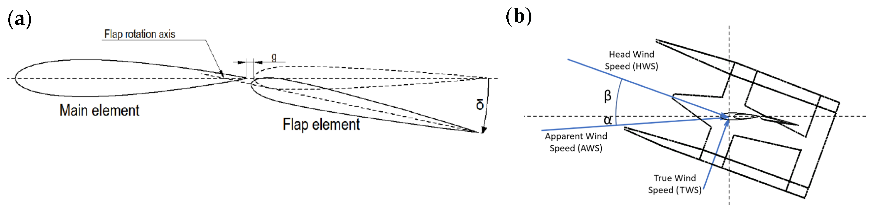
1.2. Wing Sail Operation and Basic Notations

A two-element rigid WS (Figure 1a) usually consists of a front (main element) and a rear (flap element) sail mounted on a mast [21]. This two-element wing mechanism (slotted flap) can considerably improve the propeller’s high-lift generation capability [22]. The distance between profiles (gap slot, g) is equal to 1% of the total chord length under the condition of flap deflection angle 0°, and this dimension cannot be modified during sailing. The flap can be rotated about the axis located near the trailing edge of the main element. Usually, a rigid WS is made of a symmetrical profile to provide the possibility to generate aerodynamic force on either the port or the starboard tack depending on the inflow direction. Notions concerning the velocity triangles (velocities and angles) are visible in Figure 1b.

The analysis itself was performed using several nondimensional parameters:

$${\mathrm{C}}_{\mathrm{p}}=\frac{\mathrm{p}-{\mathrm{p}}_0}{0.5{\mathsf{\rho }\mathrm{V}}_0^2}$$

(1)

$$\mathrm{CD}=\frac{D}{0.5{\mathsf{\rho }\mathrm{V}}_0^{2}A}$$

(2)

$$\mathrm{CL}=\frac{L}{0.5{\mathsf{\rho }\mathrm{V}}_0^{2}A}$$

(3)

where C_p is the pressure coefficient, p is the pressure, p₀ is the reference pressure (equal to 101,325 Pa = 1 atm), ρ is the density, and V₀ is the average reference (inlet) velocity. CD and CL are drag and lift coefficients, respectively. A is the reference area and equal to the WS chord time span.

Finally, to ensure flow similarity, the Reynolds number was kept at values corresponding to the values experienced in real life. This was achieved by the proper choice of both the chord and reference velocity values (see Table 1).

2. Numerical Methods

The presented research was conducted using two- and three-dimensional numerical simulations. Viscous Reynolds-averaged Navier–Stokes (RANS) approach was applied using k-ω SST turbulence closures with standard parameters [16]. A steady-state formulation with pseudo-transient under-relaxation was used. A fully turbulent, incompressible flow of ideal gas (dry air at 25 °C, see

Table 2. Selected fluid (air) properties set in the simulation [23].

Dynamic viscosity µ	1.831 × 10−5 kg∙m−1∙s−1
Density ρ	1.185 kg∙m−3
Molar Mass	28.96 kg∙mol−1

) was considered. All simulations were isothermal. For all simulations, second-order/high-resolution schemes were incorporated in the solution of the governing equations (continuity and momentum conservation and turbulent quantities transport equations). Single precision solvers were used: ANSYS CFX for 2D modelling (deemed more appropriate for the aerofoil simulation due to its robustness) and ANSYS Fluent for 3D analysis (as it offers easier customisation and supports overset meshes).

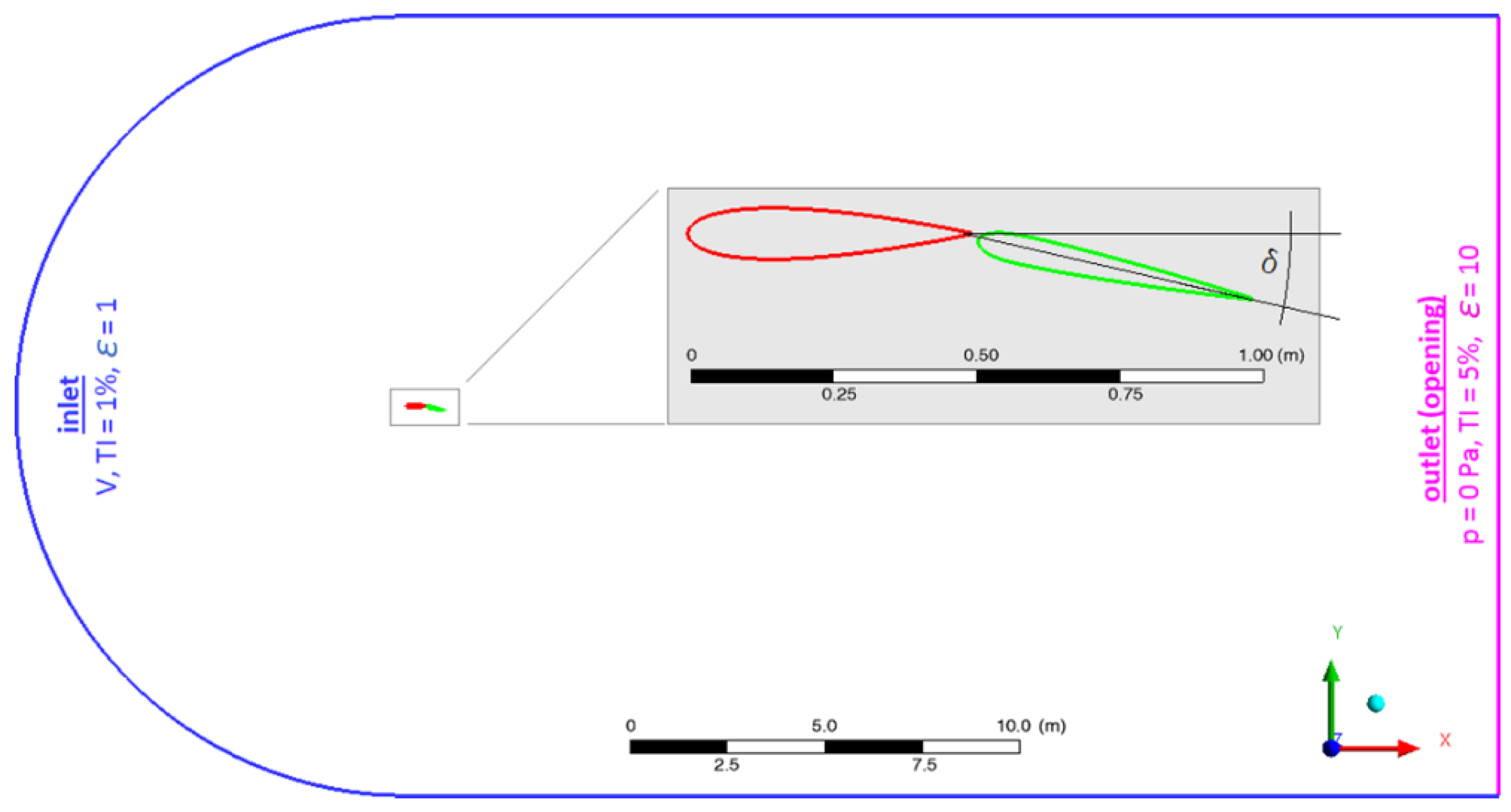
2.1. Two-Dimensional Simulation

The 2D domain enclosed a two-element cut section of the wing sail (Figure 2). The mainsail chord was aligned with the X axis, and the flap was deflected by angle δ. Because ANSYS CFX is inherently limited to 3D problems [16], one grid element (0.001 m) was extruded in the direction perpendicular to the flow (hence, the problem was formally pseudo-2D, equivalent to a wing sail of infinite span). The domain was meshed with unstructured, hex-dominant mesh swept one element along Z direction (Figure 3). The boundary conditions are shown in Figure 2.

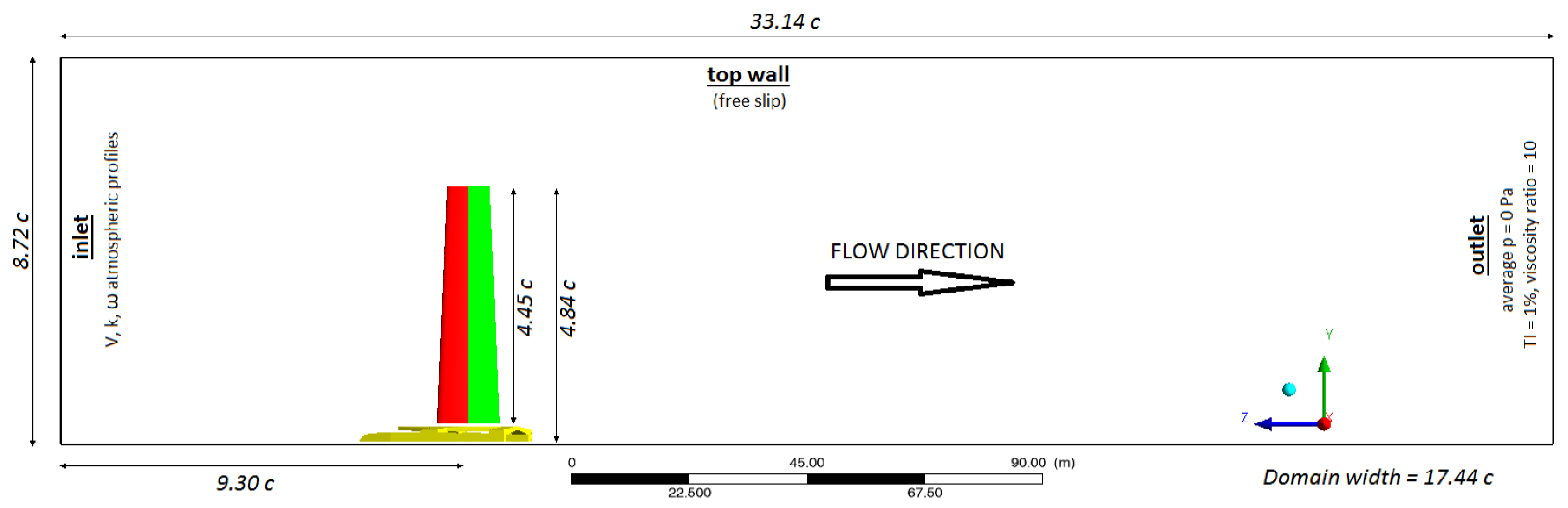
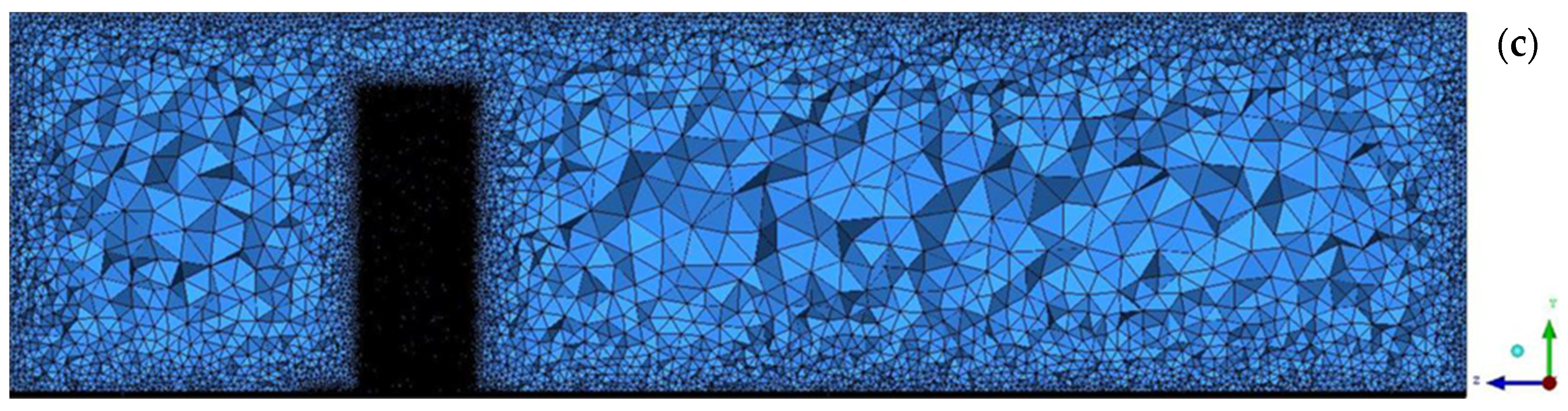
2.2. Three-Dimensional Simulation

The 3D domain (Figure 4 and Figure 5) contained a hull of size 14.0 m × 26.2 m × 2.9 m (width × length × height) and 2 sails. The vessel was placed in mid-width (X direction) of the domain at a heading angle β = 20° and 0.5 m above the water surface, same as it is after lift-off. The hull geometry was a simplified geometry of a racing catamaran. The reference length c = 8.6 m was the sum of chords of the main and flap sails at their mid-heights (y = 2.62 c); the sails were extrusions of these profiles, scaled up towards the bottom (to 1.2 c) and down towards the top (to 0.8 c). The mainsail chord was aligned with YZ, and the flap was deflected by angle δ = 12°.

The simulation was prepared employing the overset mesh approach, which is a contemporary method enabling users to independently create and combine several different flow domains, meshed separately [16]. Thus, it was possible to discretise different regions of interest accurately and merge them together afterwards. This resulted in a high-fidelity simulation at a reduced computational grid size. The sail domains were meshed with a structured grid and the other domains with an unstructured, tetrahedral grid. Inflation layer was applied to all no-slip walls to allow for an adequate resolution of the boundary layer flow.

The strategy applied to achieve appropriate mesh quality inside the computational volume was similar as in [24], i.e., y+ not larger than 2, preferably 1, on the walls of the investigated object (only wing sails here) and preserving mesh expansion factor less than 1.2. Such an approach is also in line with the recommendations given in the solver documentation [16].

As for the shape of the domain, the U- or C-shaped domain is standard for simulations of flow around aerofoils, as proved by studies of [25,26] or [27]. As stated by Ferrari [28], this domain shape and meshing approach enables one to obtain a better quality of grid than, for example, H and O shapes. This attitude also improves simulation stability, notably in the first iterations of the simulation. The mesh overview is shown in Figure 6, while the boundary conditions (BCs) are presented in Figure 4. At the inlet, an atmospheric boundary layer profile (power law with exponent B = 1/7) was imposed with true wind speed Vw = 9 m/s at reference height y0 = 27 m (Formula (4)). Increased mesh density at the inlet and outlet proved to improve the stabilisation of the simulation (especially during the first iterations). Turbulence intensity TI = 1%, and eddy viscosity ratio ε = 20 [29]. To account for the yacht movement, the velocity profile also incorporated head (boat) wind speed Vh depending on the angle of attack α. The velocity resultant from the application of Formula (4) is a real-life “twisted flow” pattern (see, e.g., [30]).

$$\begin{array}{c}{V}_i\left(y,\alpha \right)=V_{wi}\times {\left(\frac{y}{y_0}\right)}^B+V_{hi}\left(\alpha \right)\\ \begin{array}{ccc}k\left(y\right)=k_0\times {\left(\frac{y}{y_0}\right)}^B& with& k_0=\frac{2}{3}{\left(V_w\times TI\right)}^2\\ \omega \left(y\right)={\omega }_0\times {\left(\frac{y}{y_0}\right)}^B& with& {\omega }_0=\frac{\rho \times k_0}{\mu \times \epsilon }\end{array}\end{array}$$

(4)

In order to limit the artificial creation of k in the region between two sails and the hull, Menter and Kato–Lauder production limiters were applied [16].

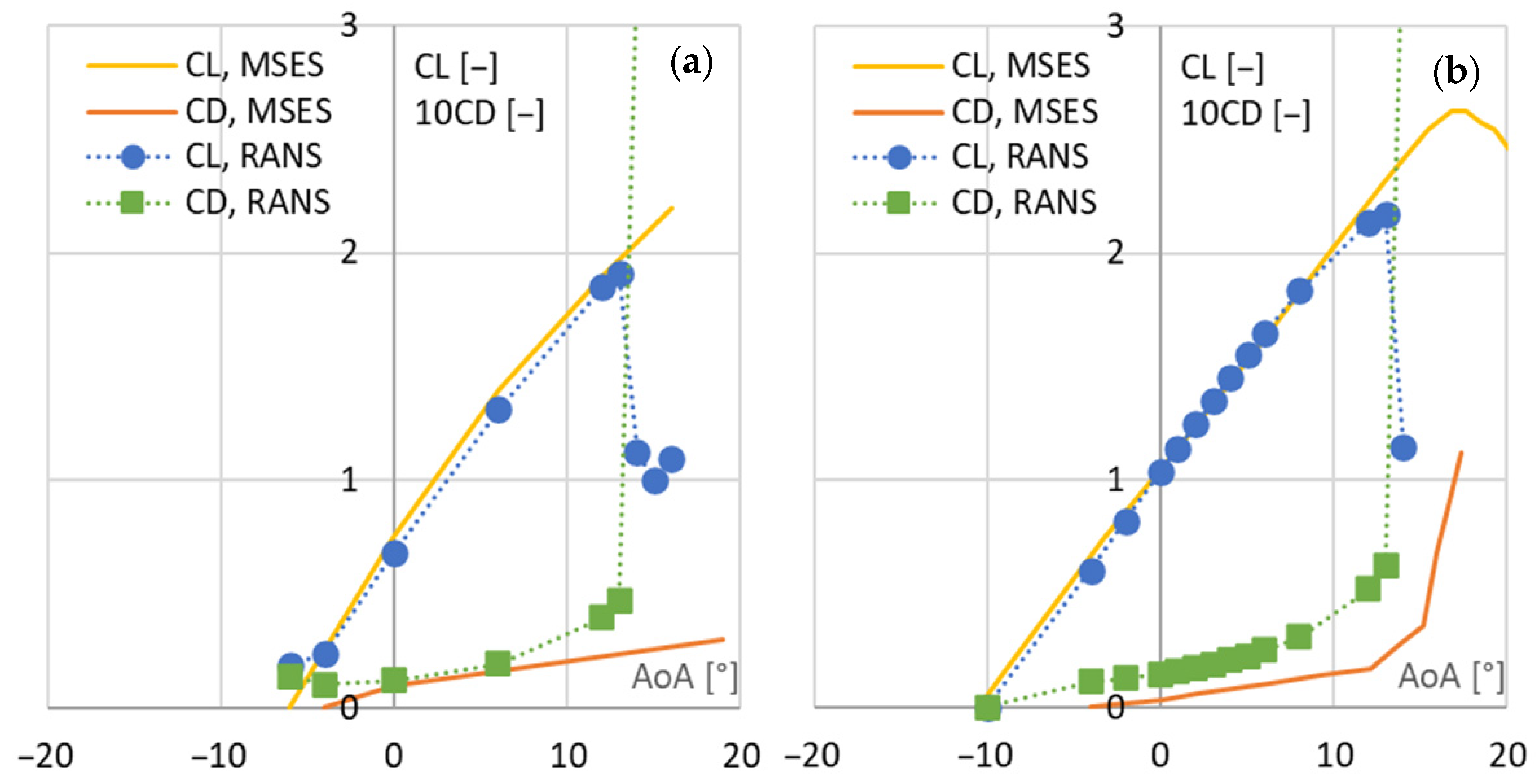
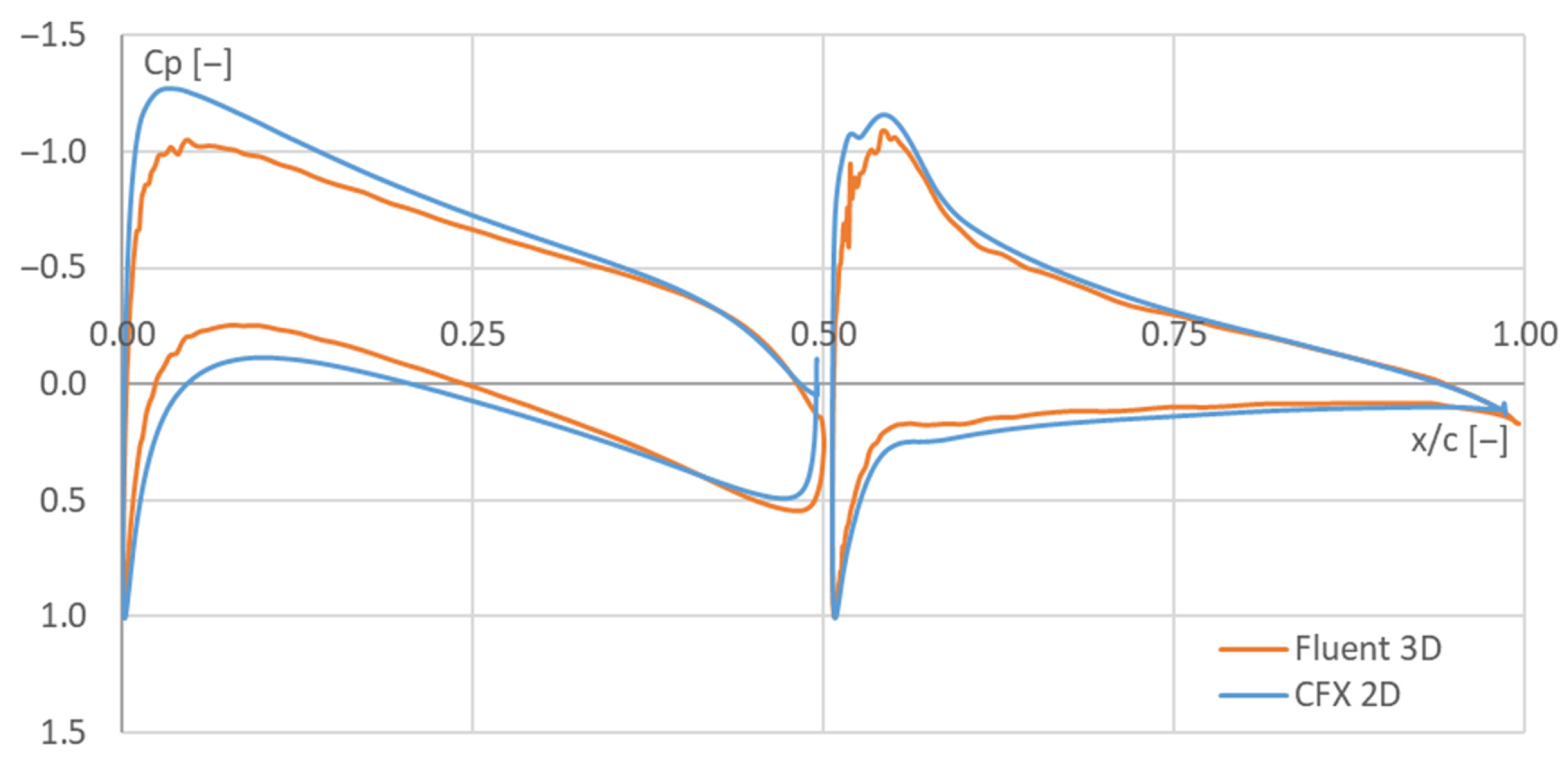
2.3. Model Verification

The general difficulty of performing full-scale WS experimental tests makes it virtually impossible to perform a detailed validation at Reynolds number ranges considered in the current study. The decision was made to prepare the model following the best practice rules, verify its numerical correctness, and, if possible, compare with existing similar numerical data.

As RANS modelling was applied, the first choice to be made was turbulence closure. Following a study of the literature and our own experience ([31,32]), k-ω SST was selected as the appropriate choice for this subsonic, external aerodynamics problem. Two-dimensional simulation was also verified for the influence of laminar–turbulent transition effects by employing the γ–Re turbulence transition model. The total aerodynamic force on WS was, in this case, approximately 1.5% lower than for fully turbulent simulation. This difference was deemed small enough to be neglected, especially in light of the extended computation time due to two additional transport equations to be solved, and the flow was thus considered fully turbulent [10,13]. These choices impose a proper range of dimensionless wall distance y+. As seen in Figure 7, the values of y+ at the sails were maintained at a level lower than approximately 2, which ensured a satisfying solution quality in their boundary layer [16,33]. As for the hull in the 3D simulation, the inflation layer in that region was adapted to avoid the buffer zone and take advantage of wall functions, i.e., targeting y+ > 50 [16].

Concerning the simulation convergence, significant discrepancies existed between various considered cases. In 2D simulation, the RMS values of the mass flow and momentum equation residuals fell well below the level of 10⁻⁷, with the exception of the stall- and post-stall flow conditions. In the latter case, the RMS equation residuals remained at the level of 10⁻⁵–10⁻³ and experienced high fluctuations, as did the monitored aerodynamic forces. This resulted from the unsteady nature of the separated flow. Under these flow conditions, steady-state, 2D simulation loses its robustness and may only be considered as a source of qualitative, rather than quantitative data. However, these flow conditions are beyond the interest of the present study as they are highly unfavourable in actual yachting. Considering the 3D analysis, the convergence was slightly poorer due to the higher case complexity and the different pressure–velocity coupling scheme. The continuity equation RMS residuals levelled off at approximately 10⁻⁴, while the velocity was less than 10⁻⁵ in all the considered cases. These levels may be judged appropriate for engineering-grade simulation, proving that the obtained results can be assumed reasonably accurate [16].

As stated previously, due to the general scarcity of accurate benchmark figures, any comparison of the obtained results with external data would be very limited. The outcomes of a similar analysis by Grassi et al. [17] employing a low-order MSES 2.8 software for high-lift multielement aerofoils [34] are compared with the 2D simulation in Figure 8. The MSES system is a collection of programs for analysis and design of single- or multielement aerofoils created at the MIT Department of Aeronautics and Astronautics. It enables prediction of lift and drag, boundary layer separation, and transition for both types of aerofoils. While both lift characteristics are coherent in the linear region, MSES predicts stall at much higher AoA. A similar phenomenon was observed and stated by Grassi et al. [17], while Duraisamy et al. [35] also underlined that k-ω SST RANS may predict stall too early. However, as stated before, the stalled flow is not of principal interest in the current research. Concerning the drag coefficient, the RANS-obtained values were universally much higher than those obtained from MSES. Closer observation of the pressure distribution on the aerofoils traced this discrepancy back to overestimation of underpressure zone near the flap tip by MSES. This again has been observed by other researchers [17,20] and associated with inaccurate predictions of the gap slot flow under certain Re conditions. The values of minimum CD obtained with RANS simulation tended to be more realistic compared to “typical” aerofoil performance (compared with [36]).

In the last step of the model analysis and verification, the 2D and 3D results were compared, as shown in Figure 9. The Cp distributions followed roughly the same trace, with some discrepancies near the leading edge of the consecutive sails up to approximately 25% x/c. One reason for this may be the difference between the number of elements across the aerofoil chord. In the case of two-dimensional simulation, the element number along the aerofoil contour was 10 times larger than in the three-dimensional model. Such a distinct leading-edge peak was not observed in the spatial calculations. However, the 3D effects (induced vortices, higher turbulence, and nonuniform inflow) could have influenced the airflow in the initial chord span, resulting in further discrepancies with respect to the 2D analysis. Similarly, the complex 3D effects in the gap slot between wing sails might have had a significant influence on the Cp over the flap element, notably near its leading edge.

In all, the model verification proves that the simulations are capable of providing consistent data concerning flow around the wing sail as long as they are conducted in the prestall conditions. More external validation data could help to validate the model in off-design wing sail operation conditions, but this is beyond the scope of the present research.

3. Results and Discussion

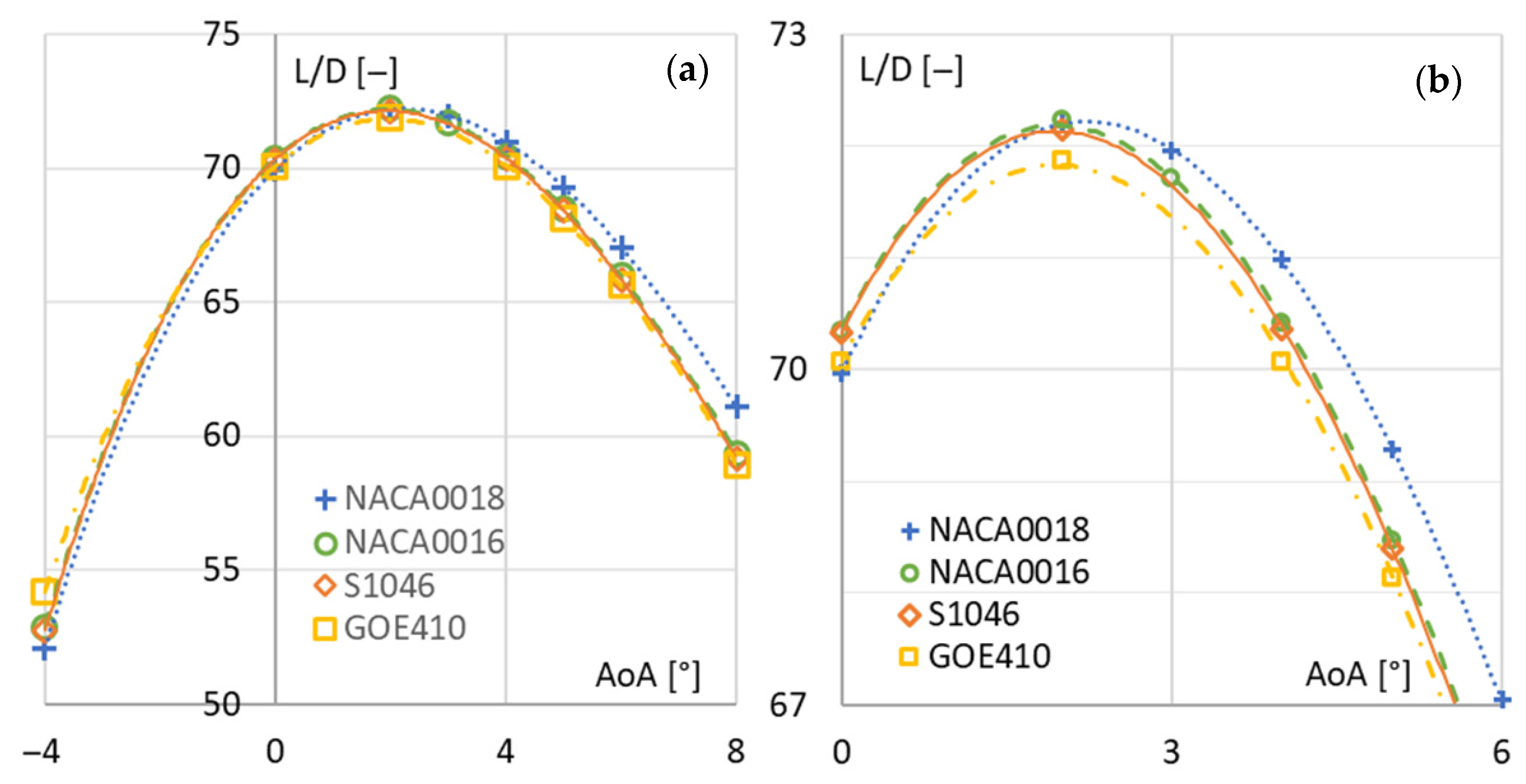
3.1. Wing Sail Performance—Comparative Study and Analysis

The examination of lift and drag coefficients was performed in 2D and 3D in order to check the performance of different WS systems at typical sailing conditions. The analysis concentrated on the flap deflection angle equal to 12°, similar to the approach presented by Grassi et al. [17]. In both 2D and 3D methodologies, higher lift coefficient and smaller drag coefficient were seen for the main element compared to the flap (Figure 10). The reason for these effects lies in the mutual influence of both elements. The flap element, placed downstream of the mainsail and exposed to a higher angle of attack, experiences unfavourable airflow conditions. Consequently, a significant reduction in CL and increase in CD occurs, meaning that the flap merely contributes to the overall sail efficiency, as has been mentioned above. Taking into consideration both wing sail elements separately, one can notice negative values of CD in the mainsail. Once again, this may be attributed to the mutual influence of the sails, the resultant pressure distribution, and profile drag. The flap element deepens the underpressure field and expands it over the suction side of the main element. Thus, thanks to the presence of the flap, the main aerofoil’s performance can be substantially altered. The aforementioned conclusions are in line with the extensive sloop sail investigations performed in [3,20]. This is manifested by the fact that as the head sail is in the upwind position, the flow over it is unobstructed and not influenced by any obstacle (for instance, a mast like in the case of the mainsail). Additionally, the presence of the flap compels the flow on the windward side to act more greatly on the pressure side of the main element (i.e., the flap element “pushes” more air towards the windward side of the main element). While the flap element in itself may increase the sail system’s drag, it has a strong contribution to the wing sail operation while being crucial for suitable trimming and manoeuvring the unit. In line with Collie et al. [20], this may be explained by the fact that the slot between the sails enables re-energising of the boundary layer flow on the leeward side of the flap as the latter is being rotated. Collie et al. [20] also obtained similarly increased performance of the system, with the maximum CL value shifting from a range 1.2 to 1.6 (symmetrical single sail system) to even 3.0 (two-element wing sail).

A convenient parameter for assessment of any profile’s aerodynamic performance is the lift-to-drag ratio (L/D). Figure 11 shows the 2D analysis results for four wing sail systems sharing the same flap element geometry. The differences in L/D are minor, which provides evidence that more profound changes in the main element geometries should be made in order to improve the performance of the unit. These may be variations in the leading-edge radius, trailing-edge wedge shape, location of the maximal thickness with respect to chord length, etc. As is clearly visible, the peak L/D value was always in the range AoA = 0–5°, which, in the future, can reduce the number of spatial calculations for new geometries. While the highest L/D was observed for NACA 0016 (AoA = 2°), in practice, it is equally important to maintain possibly high values of L/D over a wide range of AoA. In actual sailing conditions, it is practically impossible to adjust sails strictly to certain AoA, and a wide range of wing sail operation plays an important role here. Therefore, it is actually NACA 0018 whose performance may be judged as superior to NACA 0016. The 3D calculations provide further insight into the relatively wide range of AoAs, resulting in relatively high L/D values for the WS system with NACA 0018 (Figure 12). Results of the 3D calculations of the most optimal AoAs range were in line with the abovementioned 2D case, i.e., for AoA = 0–5°. This provides additional evidence that for the sake of investigation of the best WS geometry, it is plausible to perform more cost-efficient 2D analyses and only employ their results into more detailed, 3D spatial simulations.

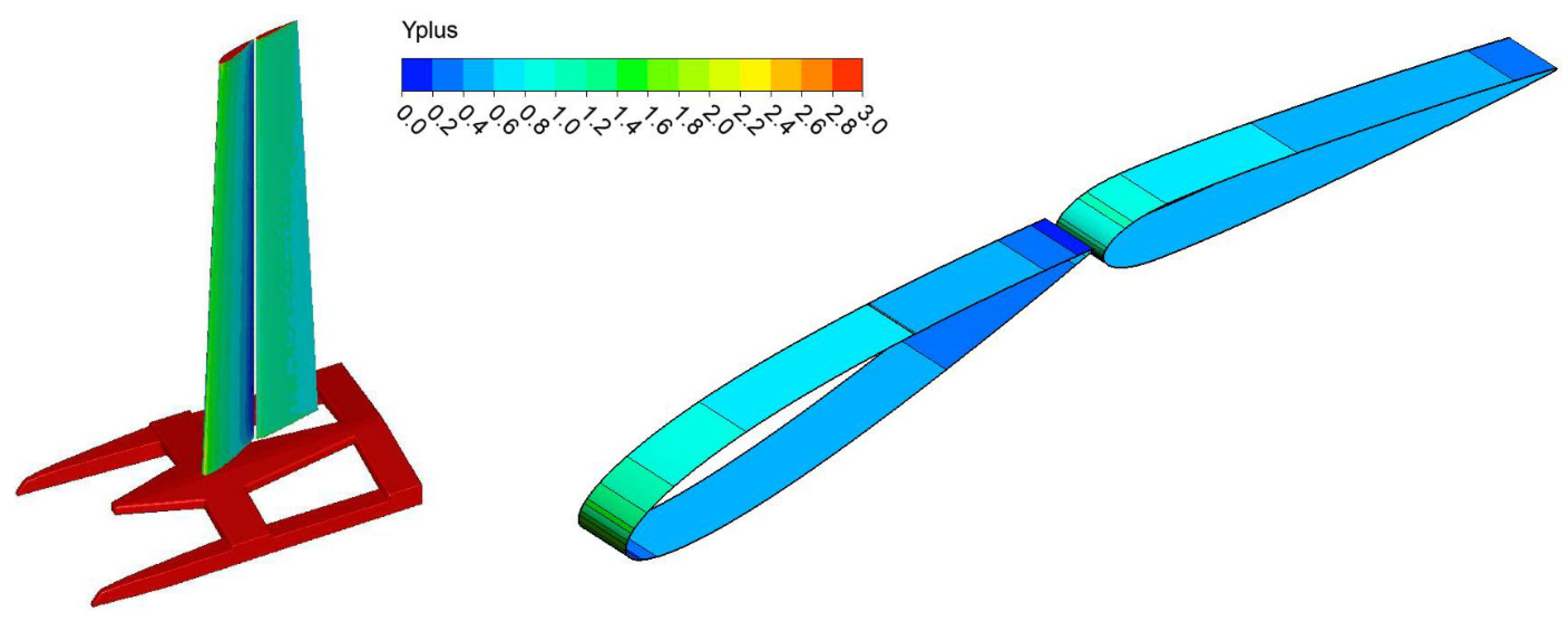
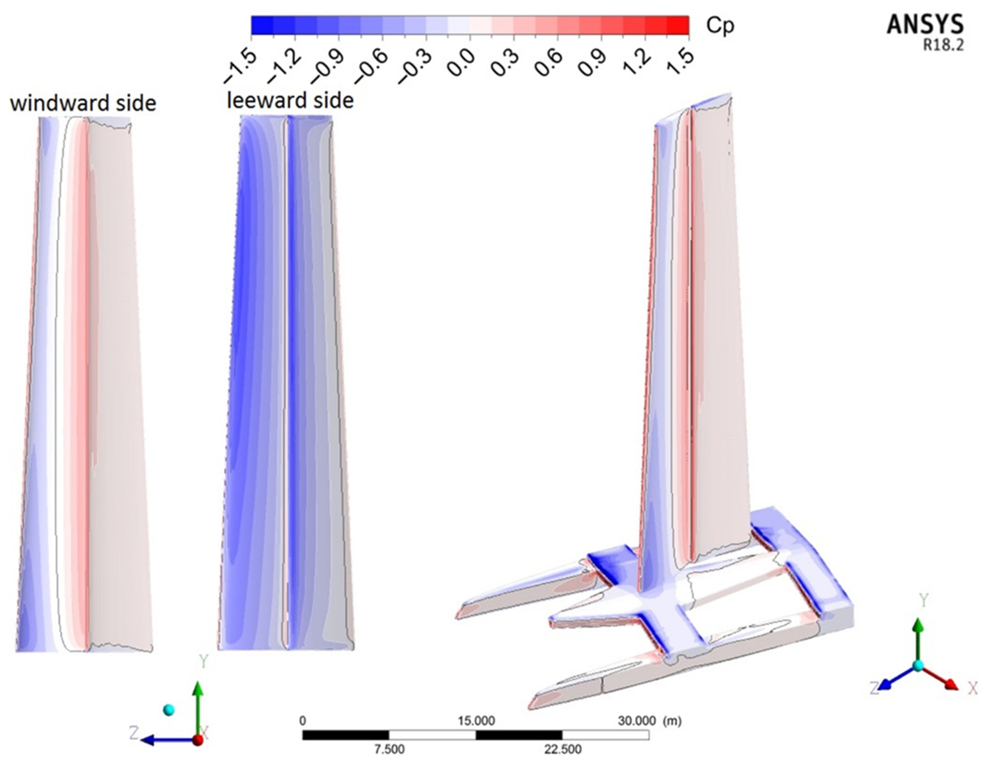
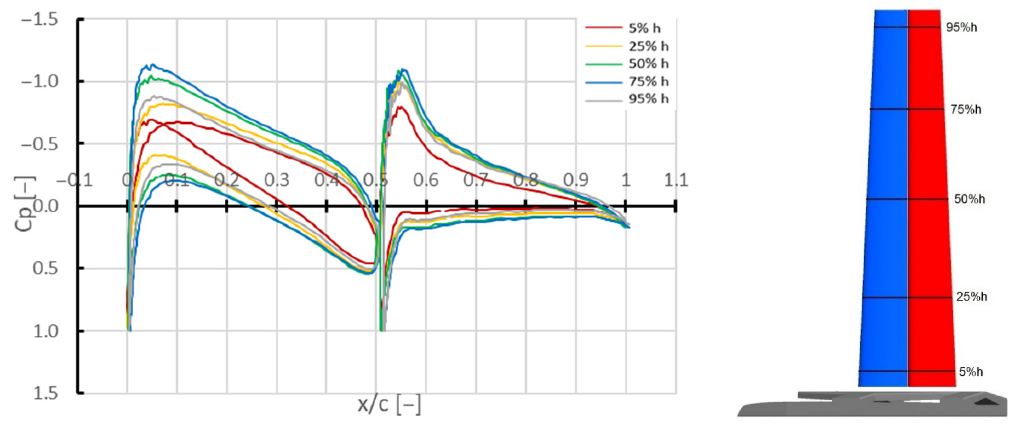
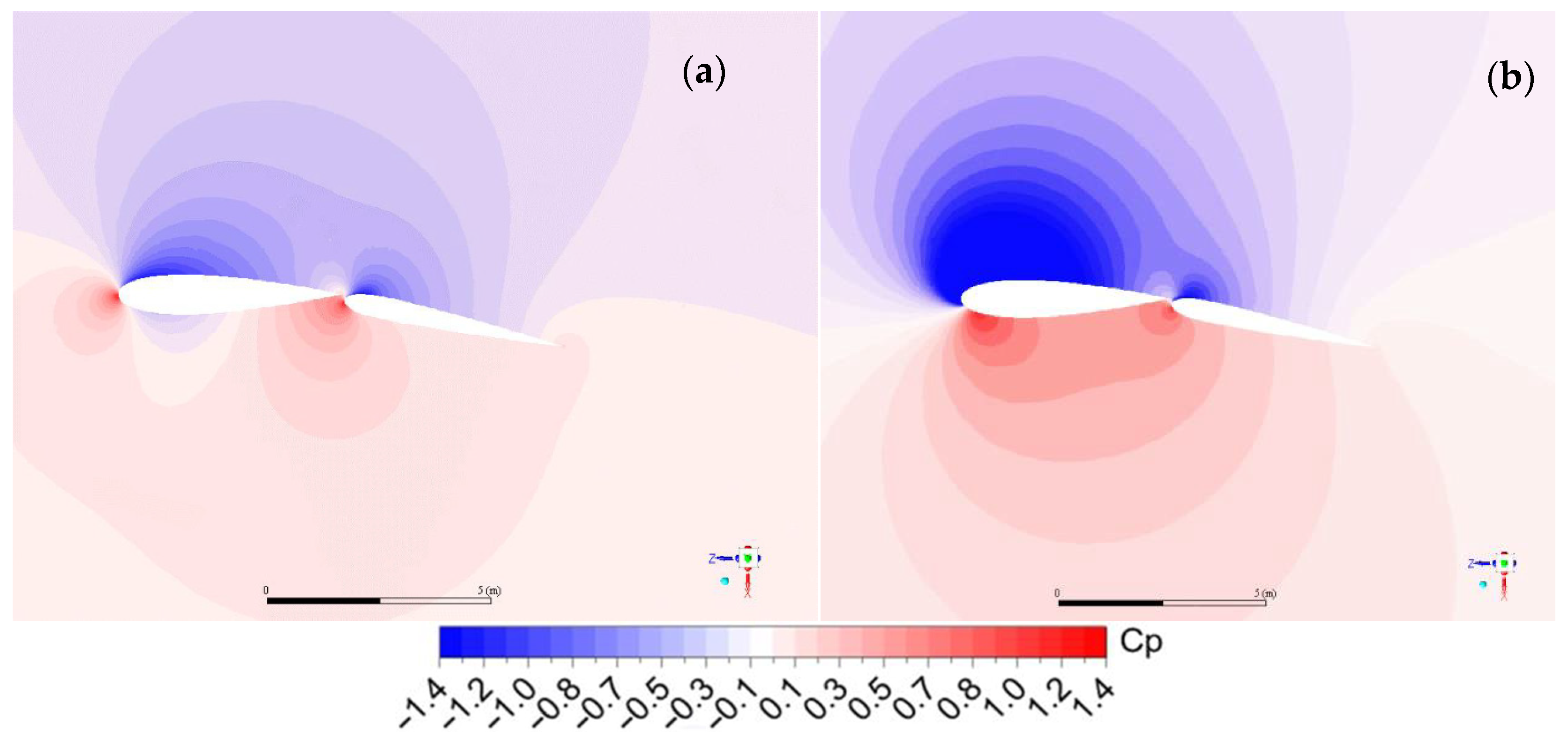
3.2. Flow around a 3D Wing Sail System

The analysis of flow fields around the yacht was performed for the uniform motion case in 3D simulations. By juxtaposing the drive force and the total drag of the boat with respect to AoA, it is possible to investigate the motion character of the unit. The drive force can be obtained by taking appropriate components of the aerodynamic forces acting on the yacht. The total drag is the sum of drag forces due to hydrofoils, aerodynamic action of appendages (only steering rudders in this case), and a variety of different aerodynamic obstacles (the crew, winches, lines and cables, etc.) [3]. The first drag component was evaluated utilising the relationship between the force enabling the yacht to take off above the water, the displacement of the unit (5400 kg), and its velocity [37]. The second and third drag components were assessed based on the study by Hagemaister and Flay [38]. Together, they contributed to around 10% of the aerodynamic drag predicted by the numerical model. The balance point of these forces specifies the AoA for which the yacht would operate under the apparent uniform motion (Figure 13). The term “apparent” here indicates that this motion characteristic is analysed under the condition of foiling, namely, “flying” of the yacht. Therefore, it can be considered that in specific wind conditions, the boat can foil and hence accelerate. In the case of this analysis, this point was in the vicinity of AoA = −8°, which can be regarded as resulting in the uniform motion conditions of the yacht. Nevertheless, as noted by Hagemaister and Flay [38], the underestimation of the drag (directly influencing the force balance) due to the hydrofoils and the nonstationary phenomena may be an important issue in studying the yacht motion.

Taking into account the abovementioned observations, it can only be assumed that the actual point of uniform motion of the yacht is shifted towards higher values of AoA, which is associated with potential increase in the total drag of the boat. Juxtaposing these results and observations with the VMG (velocity made good) graph for AC72 (see, e.g., analysis of Lisboa TIMED Race 2015 [39]) validated the feasibility of the uniform motion. Angle of attack measured with respect to the main element chord (AoA = −8°) plus heading angle (β = 20°) and additional drag estimation gave apparent sailing angle associated with the yacht axis, attaining values in the range of 15°–20°. Taking the median value as 17° (and hence AoA = −3°) from that range, one can consider it as a plausible value in the case of high-performance units. The wing sails were set as in close-hauled courses with respect to the apparent wind. Consequently, under this condition, the yacht velocity HWS was equal to 29.4 m/s and TWS was 9 m/s, thus giving the HWS/TWS ratio value of 3.26 (which, again, is a reasonable value for an AC72 [37]).

Investigation of forces acting on the yacht versus various TWS (Figure 13) led to additional observations. Firstly, with the increase in TWS, the drive force of the yacht significantly increased (even by 20% per 1 m/s of TWS). Secondly, for AoAs > −3°, there were no significant discrepancies between total drag values for consecutive AoAs. These two facts show a great advantage of foiling in the case of such units. The large increase in drive force was attained at a relatively small drag cost. The values of the drive force also possessed a relatively stable characteristic in this region. Thirdly, at AoA = −9°, the drive forces for the investigated cases were similar (they differed by no more than 1%). Here, the yacht was not under the condition of foiling; hence, the numerical model and the abovementioned assumptions were no longer relevant. The drag force was significantly larger than the drive force, resulting in at least one hull being immersed rather than “flying”. From that point on, towards lower AoAs, all the calculations of drag would have to include additional components of the immersed surfaces of the boat. For this reason, no further analysis was conducted for AoAs smaller than −9°.

Figure 14 depicts the pressure coefficient Cp distribution on yacht and wing sail surfaces at AoA = −3°. One can observe high Cp values located near the leading edges of both elements. This is even more visible in Figure 15, where the pressure coefficient distributions are plotted at five different sail elevations. The highest values of pressure coefficient were for vertical locations at the mid-span of the wing sail and above (approximately 50–75% of the height). This observation is peculiar to untwisted wing sail systems (i.e., constant flap deflection at all elevations). Taking into account the atmospheric boundary layer and the resulting apparent wind, more energy is delivered to the wing sails at higher levels. This effect is not favourable, as it increases the rolling moment of the yacht; therefore, in practice, a twisted WS may be used. However, in this study, the centre of pressure was expectedly within the abovementioned region, which is coherent with observations presented in [17]. At 25% and 95% of wing sail height, there was a significant decrease in Cp in the case of the main element, followed by a further slight drop on the flap element. This is related to the wing tip effects, which results in induced drag generation. An even deeper decrease in Cp on the wing sail pressure side was visible at 5% of its height. This can be attributed to the influence of the hull. The catamaran body, composed mainly of two hulls and the connecting midship, significantly affects the flow character. It divides it into two “streams”: the flow above and below the body. As the “upper flow stream” is not so influenced by the water surface and components of the hull (as it is in the case of the lower flow, bounded by the hulls and midship), it is free to accelerate. This, in turn, provokes a reduction of the (static) pressure coefficient at the bottom of the wing sail. A more profound understanding of the influence of air flow around a hull on the yacht performance could possibly bring further improvements in this field but is beyond the scope of the current research.

Comparing pressure fields at midplane of the wing for AoA = −3° and AoA = 12° (Figure 16), a major change in the distribution could be seen. At higher AoA, the stagnation points moved significantly towards the pressure side and a larger underpressure region appeared on the suction side. This can cause generation of larger drive force; consequently, the yacht accelerates.

Regarding the relative velocity distribution at AoA = −3° and AoA = 12° (Figure 17), some differences can be also spotted. At AoA = 12°, lower velocity magnitudes were moved further into the pressure side of the system. Looking at the wake, it was considerably wider for the latter case (AoA = 12°). This behaviour is connected with the higher angle of attack of the flow. There was no flow separation, which once again proves that the stall did not occur before AoA = 12°.

The gap slot used in this simulation did not trigger flow separation on the flap suction side at the considered AoA range, which is in line with the study elaborated in [22]. A gap slot too wide may lead to a decrease in pressure difference between the pressure and suction sides of the system and cause a decrease in sail efficiency (as described extensively in [40,41]). The behaviour of the airflow passing the gap slot remained similar for all AoAs and elevation cases. The only visible difference was the slight displacement of the flap element stagnation point in the vicinity of the flap element leading edge.

4. Conclusions

In this study, CFD modelling of a rigid wing sail for a high-performance yacht is presented. In the first stage, a two-dimensional method was developed, which was proven to account for flow phenomena similar to real flow acting on the unit. Apparently, even minor changes in the aerofoil thickness (NACA 0016) or slight differences in the shape (GOE410 and S1046) affect the performance of the system. Moreover, the 2D analyses gave valuable insight into the more detailed AoA ranges and flap deflection adjustment, where the best operating conditions can be sought. In elaborated cases, the characteristics of NACA 0018 aerofoil as a main element depict the great potential for further improvement of such propulsions systems, provided δ is equal to 12°.

Regarding the spatial analyses, an appropriate numerical model based on the overset discretization approach was created with success. A propulsion system equipped with NACA 0018 aerofoil (main element) and unchanged cross-sectional shape of the flap element was investigated in the presence of real value of Re (c.a. 7 × 10⁶–25 × 10⁶). The hull shape was based on the AC72 yacht. The main objective of the 3D model was to investigate the flow around the unit and its dynamics in order to compare these features with other studies, both numerically and experimentally. The analysis of uniform motion of the vessel was performed so as to compare it with VMG plots specific for AC72 units. As a result, the obtained similarities provided further evidence of the fidelity of the numerical model. Based on the analyses of factors such as Cp, CL, CD, and L/D ratio, conditions of the uniform motion of the vessel were determined. The most plausible sailing conditions with the elevated L/D ratio value were recorded for around AoA = −3°. The investigated unit maintained relatively high CL and modest CD values in a wide range of AoAs (from −3° to 9°). All considered cases were at prestall condition, i.e., there was no evidence of nonstationary flow characteristic. The stall phenomenon could have been observed for higher AoAs. The hull geometry influenced the flow characteristic and Cp in the lower parts of the wing sail system. This indicated the relevance of including the hull in the flow analysis, especially in terms of wing sail performance assessment. The significant advantage of the presented model is the overset method, which provides substantial flexibility in mesh generation. This can considerably reduce workload and preparation time in future research. It is also important that the use of overset meshes in the current study did not reduce the simulation fidelity or stability, even in the complex flow regions in the sail gap or near the water. Moreover, as the wing sail system is only one of many devices used on a yacht, employing the overset approach to easily adapt and exchange other vessel elements can also be advantageous.

The presented methods, obviously not flawless, provide a firm starting point that can be utilised in further wing sail analyses and applied in the development process of other devices, e.g., hydrofoils, rudders, hulls, etc. Although tackling only the WS system may not be a game-changer, surely, utilising elaborate methods in the case of other components can eventually alter the result of the game.

References

1. America’s Cup Race Management. America’s Cup “72” Class Rule; ACRM, 2010. Available online: https://web.archive.org/web/20131001060304/http://noticeboard.americascup.com/governing-documents/ac72-class-rule/ (accessed on 1 November 2023).
2. Associated Press. Kiwis Reach Record Speed in AC 72-Foot Catamaran; NBC Universal Media, 2013. Available online: https://www.nbcbayarea.com/news/sports/kiwis-reach-record-speed-in-ac-72-foot-catamaran/1949645/ (accessed on 1 November 2023).
3. Marchaj, C.A. Sail Performance: Techniques to Maximise Sail Power; Adlard Coles Nautical: London, UK, 2003. [Google Scholar]
4. Larsson, L.; Eliasson, R.; Orych, M. Principles of Yacht Design; A&C Black: London, UK, 2014. [Google Scholar]
5. Lee, H.J.Y.; Lee, D.-J.; Choi, S. Surrogate model based design optimization of multiple wing sails considering flow interaction effect. Ocean. Eng. 2016, 121, 422–436. [Google Scholar] [CrossRef]
6. Oxford Essential Dictionary of the, U.S. Military; Oxford University Press: Oxford, UK, 2001. [Google Scholar]
7. Ariffin, N.I.B.; Hannan, M.A. Wingsail technology as a sustainable alternative to fossil fuel. IOP Conf. Ser. Mater. Sci. Eng. 2020, 788, 012062. [Google Scholar] [CrossRef]
8. Silva, M.F.; Friebe, A.; Malheiro, B.; Guedes, P.; Ferreira, P.; Waller, M. Rigid wing sailboats: A state of the art survey. Ocean Eng. 2019, 187, 106150. [Google Scholar] [CrossRef]
9. Sail-World Australia. America’s Cup-Oracle Team USA Emerges Victorious. 2013. Available online: https://www.sail-world.com/Australia/Americas-Cup-Oracle-Team-USA-emerges-victorious/-115062 (accessed on 7 January 2024).
10. Chapin, V.; Gourdain, N.; Verdin, N.; Fiumara, A.; Senter, J. Aerodynamic study of a two-elements wingsail for high performance multihull yachts. In Proceedings of the 5th High Performance Yacht Design Conference, Auckland, New Zealand, 10–12 March 2015. [Google Scholar]
11. Fiumara, A.; Gourdain, N.; Chapin, V.; Senter, J.; Bury, Y. Numerical and experimental analysis of the flow around a two-element wingsail at Reynolds number 0.53 × 10⁶. Int. J. Heat Fluid Flow 2016, 62, 538–551. [Google Scholar] [CrossRef]
12. Fiumara, A.; Gourdain, N.; Chapin, V.; Senter, J. Aerodynamic Analysis around a C-Class Catamaran in Gust Conditions using LES and Unsteady RANS Approaches. In Proceedings of the International Conference on Innovation in High Performance Sailing Yachts INNOVSAIL, Lorient, France, 28–30 June 2017. [Google Scholar]
13. Fiumara, A.; Gourdain, N.; Chapin, V.; Senter, J. Aerodynamic analysis of a C-class-like catamaran in simplified unsteady wind conditions using LES and URANS modeling. J. Wind. Eng. Ind. Aerodyn. 2018, 180, 262–275. [Google Scholar] [CrossRef]
14. Bordogna, G.; Keuning, J.A.; Huijsmans, R.H.M.; Belloli, M. Wind-tunnel experiments on the aerodynamic interaction between two rigid sails used for wind-assisted propulsion. Int. Shipbuild. Prog. 2018, 65, 93–125. [Google Scholar] [CrossRef]
15. Khaware, A.; Gupta, V.K.; Punekar, H.; Sharkey, P. Numerical Simulation of Ship Motion and Life Boat Launch using Overset Mesh. In Proceedings of the 11th International Workshop on Ship and Marine Hydrodynamic, Hamburg, Germany, 21–24 September 2019. [Google Scholar]
16. ANSYS. ANSYS Fluent 18.2 Theory Guide; Ansys Inc.: Canonsburg, PA, USA, 2017. [Google Scholar]
17. Grassi, C.; Foresta, M.; Lombardi, G.; Katz, J. Study of rigid sail aerodynamics. Int. J. Small Craft Technol. 2013, 155, 13–24. [Google Scholar]
18. Foresta, M.; Grassi, C.; Katz, J.; Lombardi, G. Lift and Drag Measurements of Tandem, Symmetric Airfoils. In Proceedings of the 31st AIAA Applied Aerodynamics Conference, San Diego, CA, USA, 24–27 June 2013. [Google Scholar]
19. Fiumara, A.; Gourdain, N.; Chapin, V.; Senter, J. Comparison of wind tunnel and freestream conditions on the numerical predictions of the flow in a two elements wingsail. In Proceedings of the AAAF 50th Applied Aerodynamics Conference (AERO 2015), Toulouse, France, 30 March–1 April 2015. [Google Scholar]
20. Collie, S.; Fallow, B.; Hutchins, N.Y.H. Aerodynamic design development of AC72 wings. In Proceedings of the 5th High Performance Yacht Design Conference 2015 (HPYD 5), Auckland, New Zealand, 10–12 March 2015. [Google Scholar]
21. Dane, R.; Mathew, N.; McBride, I. Rigid Wing Sail. USA Patent 9937987, 2 November 2016. [Google Scholar]
22. Fiumara, A.; Gourdain, N.; Chapin, V.; Senter, J. Aerodynamic analysis of 3D multi-elements wings: An application to wingsails of flying boats. In Proceedings of the Royal Aeronautical Society 2016 Applied Aerodynamic Conference, Bristol, UK, 19–21 July 2016. [Google Scholar]
23. Lide, D.R. CRC Handbook of Chemistry and Physics; CRC Press LLC: Boca Raton, FL, USA, 2004. [Google Scholar]
24. Li, C.; Wang, H.; Sun, P. Numerical Investigation of a Two-Element Wingsail for Ship Auxiliary Propulsion. J. Mar. Sci. Eng. 2020, 8, 333. [Google Scholar] [CrossRef]
25. Honarmand, M.; Djavareshkian, M.H.; Feshalami, B.F.; Esmaeilifar, E. Numerical Simulation of a Pitching Airfoil Under Dynamic Stall of Low Reynolds Number Flow. J. Aerosp. Technol. Manag. 2019, 11, e4819. [Google Scholar] [CrossRef]
26. Götten, F.; Finger, F.; Havermann, M.; Braun, C. A highly automated method for simulating airfoil characteristics at low Reynolds number using a RANS-transition approach. In Proceedings of the Deutscher Luft-und Raumfahrtkongress—DLRK 2019, Darmstadt, Germany, 29 September–1 October 2019. [Google Scholar]
27. Esmaeilifar, E.; Djavareshkian, M.H.; Feshalami, B.F.; Esmaeili, A. Hydrodynamic simulation of an oscillating hydrofoil near free surface in critical unsteady parameter. Ocean Eng. 2017, 141, 227–236. [Google Scholar] [CrossRef]
28. Ferrari, J.A. Influence of Pitch Axis Location on the Flight Characteristics of a NACA 0012 Airfoil in Dynamic Stall. Master’s Thesis, Rensselaer Polytechnic Institute, Troy, Turkey, 2012. [Google Scholar]
29. Murad, J. Defining Turbulent Boundary Conditions. SimScale, 6 November 2020. Available online: https://www.simscale.com/forum/t/defining-turbulent-boundary-conditions/80895 (accessed on 1 November 2023).
30. Viola, I.M.; Flay, R.G.J. Sail aerodynamics: Understanding pressure distributions on upwind sails. Exp. Therm. Fluid Sci. 2011, 35, 1497–1504. [Google Scholar] [CrossRef]
31. Lipian, M.; Dobrev, I.; Massouh, F.; Jozwik, K. Small wind turbine augmentation: Numerical investigations of shrouded- and twin-rotor wind turbines. Energy 2020, 201, 117588. [Google Scholar] [CrossRef]
32. Sobczak, K.; Obidowski, D.; Reorowicz, P.; Marchewka, E. Numerical Investigations of the Savonius Turbine with Deformable Blades. Energies 2020, 13, 3717. [Google Scholar] [CrossRef]
33. Bradshaw, P.; Huang, G.P. The Law of the Wall in Turbulent Flow. Proc. R. Soc. A Math. Phys. Eng. Sci. 1995, 451, 165–188. [Google Scholar]
34. Drela, M. A User’s Guide to MSES 3.05; MIT Department of Aeronautics and Astronautics: Cambridge, MA, USA, 2007. [Google Scholar]
35. Duraisamy, K.; Spalart, P.R.; Rumsey, C.L. Status, Emerging Ideas and Future Directions of Turbulence Modeling Research in Aeronautics; NASA: Hampton, VA, USA, 2017.
36. Hoerner, S.F. Fluid-Dynamic Drag; Hoerner Fluid Dynamics: Bakersfield, CA, USA, 1965; p. 455. [Google Scholar]
37. Wilkinson, N.; Kensington, A. Battle of the boats—How technology won the America’s Cup. In IPENZ Centenary Lecture Series; IPENZ: New Plymouth, New Zealand, 2014. [Google Scholar]
38. Hagemeister, N.; Flay, R.G.J. Velocity Prediction of Wing-Sailed Hydrofoiling Catamarans. J. Sail. Technol. 2019, 4, 66–83. [Google Scholar] [CrossRef]
39. Sailonline NavSim, A.B. Archived Races. 31 May 2021. Available online: http://www.sailonline.org/races/all/archive/ (accessed on 1 November 2023).
40. Blakeley, A.W.; Flay, R.; Richards, P.J. Design and Optimisation of Multi-Element Wing Sails for Multihull Yachts. In Proceedings of the 18th Australasian Fluid Mechanics Conference, Launceston, Australia, 3–7 December 2012. [Google Scholar]
41. Blakeley, A.W.; Flay, R.; Furukawa, H.; Richards, P.J. Evaluation of Multi-Element Wing Sail Aerodynamics from Two-Dimensional Wind Tunnel Investigations. In Proceedings of the 5th High Performance Yacht Design Conference, Auckland, New Zealand, 10–12 March 2015. [Google Scholar]
Figure 1. Geometry of the wing sail cross section (a) and velocity triangles (b).
Energies 17 00549 g001
Figure 2. Sectional view of the 2D domain and the boundary conditions; wing surfaces are no-slip walls, XY walls are symmetry walls, δ = 12°.
Energies 17 00549 g002
Figure 3. Global overview of the 2D mesh and zoom on the sail vicinity region (miniature).
Energies 17 00549 g003
Figure 4. Sectional view of the 3D domain and the boundary conditions; all unmarked walls are no-slip walls.
Energies 17 00549 g004
Figure 5. Yacht elements (left): hull (yellow), main (red), and flap (green) wing sail elements and their respective domains (right); main domain represented as wireframe, and water surface indicated in blue.
Energies 17 00549 g005
Figure 6. Cross-sectional view of 3D mesh around the wing sail (a), hull (b), and main domain (c).
Energies 17 00549 g006aEnergies 17 00549 g006b
Figure 7. Y+ distribution in 3D (AoA = −3°, left) and 2D simulation (NACA0016, δ = 12°, AoA = 3°, right).
Energies 17 00549 g007
Figure 8. Lift and drag coefficient—comparison of 2D simulation and reference MSES data for NACA 0016 [17], δ = 8° (a) and δ = 12° (b).
Energies 17 00549 g008
Figure 9. Cp distribution along the wing sails—2D vs. 3D simulation (at sail midspan) results for AoA = −3°.
Energies 17 00549 g009
Figure 10. CL (a) and CD (b) coefficients for separate elements and whole wing sail system.
Energies 17 00549 g010
Figure 11. Performance of different wing sail systems (main + flap), 2D simulation, δ = 12°; full range (a) and close-up (b).
Energies 17 00549 g011
Figure 12. L/D ratio for the yacht (wing sails + hull), 3D simulation.
Energies 17 00549 g012
Figure 13. Drive force and total drag plot for a considered yacht versus various TWS.
Energies 17 00549 g013
Figure 14. Cp distribution on the yacht, AoA = −3°.
Energies 17 00549 g014
Figure 15. Cp distribution at different WS elevations, AoA = −3°.
Energies 17 00549 g015
Figure 16. Pressure fields at sail midplane, AoA = −3° (a) and AoA = 12° (b).
Energies 17 00549 g016
Figure 17. Velocity fields at sail midplane, AoA = −3° (a) and AoA = 12° (b).
Energies 17 00549 g017