Article

Research on the Economic Scheduling Problem of Cogeneration Based on the Improved Artificial Hummingbird Algorithm

School of Mechanical and Electrical Engineering, Henan Institute of Science and Technology, Xinxiang 453003, China
*
Author to whom correspondence should be addressed.
Energies 2024, 17(24), 6411; https://doi.org/10.3390/en17246411
Submission received: 14 November 2024 / Revised: 13 December 2024 / Accepted: 17 December 2024 / Published: 19 December 2024
(This article belongs to the Section C: Energy Economics and Policy)

Abstract

:
With the increasing application of Combined Heat and Power (CHP) units, Combined Heat and Power Economic Dispatch (CHPED) has emerged as a significant issue in power system operations. To address the complex CHPED problem, this paper proposes an effective economic dispatch method based on the Improved Artificial Hummingbird Algorithm (IAHA). Given the complex constraints of the CHPED problem and the presence of valve point effects and prohibited operating zones, it requires the algorithm to have high traversal capability in the solution space and be resistant to becoming trapped in local optima. IAHA has introduced two key improvements based on the characteristics of the CHPED problem and the shortcomings of the standard Artificial Hummingbird Algorithm (AHA). Firstly, IAHA uses chaotic mapping to initialize the initial population, enhancing the algorithm’s traversal capability. Second, the guided foraging of the standard AHA has been modified to enhance the algorithm’s ability to escape from local optima. Simulation experiments were conducted on CHP systems at three different scales: 7 units, 24 units, and 48 units. Compared to other algorithms reported in the literature, the IAHA algorithm reduces the cost in the three testing systems by up to USD 18.04, 232.7894, and 870.7461. Compared to other swarm intelligence algorithms reported in the literature, the IAHA algorithm demonstrates significant advantages in terms of convergence accuracy and convergence speed. These results confirm that the IAHA algorithm is effective in solving the CHPED problem while overcoming the limitations of the standard AHA.

1. Introduction

Economic dispatch is one of the primary optimization problems in power system operations [1]. However, traditional power plants, which rely on coal-fired generation, suffer from low energy efficiency. During the energy conversion process, a significant amount of heat is lost and wasted. Combined Heat and Power (CHP) units improve energy conversion efficiency and avoid waste heat by generating electricity and heating simultaneously [2]. Over the years, CHP technology has garnered increasing attention from researchers due to its superior energy conversion efficiency [3,4]. According to the literature, CHP units can achieve 90% or higher energy efficiency [5] while reducing nearly 13% to 18% of pollutant gas emissions [6].
CHP systems typically consist of power-only units, CHP units, and heat-only units [7]. Due to the presence of Valve Point Effects and Prohibited Operating Zones (POZ) in traditional thermal power systems, the objective function of the Combined Heat and Power Economic Dispatch (CHPED) problem exhibits both nonlinear and non-convex characteristics [8]. CHPED aims to minimize the total production cost while satisfying various constraints, including VPE effects, power and heat generation capabilities, power-heat demand balance, and transmission losses [9].
Early studies proposed several classical mathematical methods, such as Lagrangian relaxation [10] and dual-quadratic programming [11], to address the CHPED problem. In response to these challenges, swarm intelligence optimization algorithms have gained significant attention for their ability to find optimal solutions under multiple constraints rapidly. Consequently, researchers began employing swarm intelligence optimization algorithms to tackle CHPED problems of varying scales. For example, Haghrah et al. [12] proposed an improved Real-Coded Genetic Algorithm based on Chaos Random Walk Mutation (RCGA-CRWM), introducing a simple method to determine the step sizes of random walks, which enhanced the algorithm’s convergence speed while avoiding premature convergence. Liu et al. [13] introduced a niching differential evolution algorithm (NDE) that balances the global and local search capabilities of the algorithm by using two strategies: the niching method and greedy selection, and verified its effectiveness on large-scale CHPED problems. An improved Marine Predator Optimization Algorithm (IMPOA) was proposed for the CHPED problem by Shaheen et al. [14], and its performance was tested using four testing systems to validate its efficiency and feasibility in solving CHPED problems of different scales. Ramachandran et al. [15] proposed the FRCSA-ABC algorithm by combining the Fuzzy adaptive Ranking-based Crow Search Algorithm (FRCSA) with an improved Artificial Bee Colony (ABC) algorithm. This algorithm incorporates three mechanisms that can achieve cost-effectiveness while ensuring global convergence. Sun et al. [16] introduced an Indicator & crowding Distance-Based Evolutionary Algorithm (IDBEA) specifically designed to address this non-convex and nonlinear problem. IDBEA was tested on three different types of CHPED systems. The simulation results demonstrate that the IDBEA algorithm has strong stability and superiority, and its solutions exhibit better convergence and diversity compared to other algorithms. Zhou et al. [17] proposed a novel Hybrid Neighbor Topology-based Multi-Agent Crossover algorithm (HNT-MACSO) to enhance the balance between exploration and exploitation, thereby improving the robustness of the CSO (Cat Swarm Optimization). Five CHP systems were tested, and the experimental results confirmed the effectiveness and superiority of HNT-MACSO in solving large-scale CHPED problems. Based on thermodynamics and heat transfer principles, Pattanaik et al. [18] proposed a heuristic optimization algorithm called Heat Transfer-based Search (HTS) to solve the CHPED problem, taking into account realistic constraints such as valve point effects, ramp rate limitations, and network losses. Ozkaya et al. [19] introduced a novel approach named Adaptive Fitness-Distance Balance-based Artificial Rabbits Optimization (AFDB-ARO) to address the CHPED problem. AFDB-ARO leverages the guidance mechanism of AFDB to enhance the exploration capabilities of ARO, thereby strengthening the balance between exploration and exploitation. Experimental results have confirmed the stability and superior performance of AFDB-ARO. Chen et al. [5] presented an improved Differential Evolution algorithm for large-scale CHPED problems, named SEDGCM, which enhanced performance by incorporating Gaussian-Cauchy mutation and parameter adaptation strategies, demonstrating the method’s excellent accuracy and stability in solving large-scale CHPED problems. For the non-convex and nonlinear CHPED problems in power systems, Nazari-Heris et al. [20] proposed a novel Multi-Person Harmony Search (MPHS) method. The performance of the proposed MPHS algorithm was validated on medium-scale and large-scale CHPED problems. Huang et al. [21] proposed the Heterogeneous Evolving Cuckoo Search (HECS) algorithm, which integrates learning strategies and applies heterogeneous evolutionary approaches, as well as a novel constraint handling mechanism, to tackle large-scale CHPED problems considering valve point effects. The effectiveness of HECS was proven with five CHP test systems. An improved artificial bee colony (IABC) algorithm was proposed to solve the CHPED problem by Rabiee et al. [22]. This algorithm has been applied to three testing systems, two of which are large-scale CHPED problems, demonstrating its superiority in handling non-convex and constrained CHPED problems. Spea et al. [23] employed a novel optimization algorithm, namely the Social Network Search (SNS) algorithm, to tackle the CHPED problem. SNS mimics the behavior of social network users to increase popularity, and experimental results have confirmed the effectiveness of SNS in various CHPED problems. By combining the Grey Wolf Optimizer (GWO) with Lévy Flight, Wang et al. [24] proposed the Lévy GWO algorithm, which overcomes the premature convergence problem of the GWO algorithm. They also introduced a constraint handling method, effectively solving scheduling problems that are difficult to handle due to numerous constraints.
In summary, swarm intelligence optimization algorithms can solve most optimization problems. However, it is important to note that no single intelligent optimization algorithm can efficiently solve all types of optimization problems and always find the best solution [25,26]. Therefore, it is necessary to combine real-world problems, improve existing swarm intelligence optimization algorithms, and explore more suitable solutions to problems.
The Artificial Hummingbird Algorithm (AHA) was introduced as a powerful algorithm by Weiguo Zhao, Liying Wang, and others in 2021 [27]. Their research indicates that AHA is a continuous algorithm that demonstrates good performance in the global optimization of complex functions. Due to its suitability for solving highly complex, non-convex problems that require high precision, it has been widely applied. As demonstrated in the literature [28], the AHA algorithm is applied to solve the complex problem of coordinated wind–solar–thermal generation scheduling problem in a multi-objective framework. The CHPED is a continuous problem, and in the actual situation, we often need to consider the fuel costs of three different types of units simultaneously, as well as the challenge of prohibited operating zones. Therefore, the CHPED problem is very complex and non-convex, requiring high traversal capability in the solution space and the ability of the algorithm to escape local optima. AHA, as a continuous algorithm, has a unique access table mechanism, flight patterns, and foraging behavior, which can help hummingbirds quickly and effectively find the optimal solution to highly complex and continuous problems. The characteristics of AHA are very consistent with those of the CHPED problem, so this paper employs AHA to solve the CHPED problem.
However, AHA suffers from drawbacks such as insufficient ergodicity and population diversity due to random initialization. Additionally, during the process of guiding foraging, if the fitness value of the new food source is poor, the guidance tends to be ineffective, resulting in the AHA easily falling into local optimality. To address these shortcomings, this paper first introduces chaotic mapping to initialize the population, improving the algorithm’s ergodicity and diversity. Secondly, the update mechanism of the AHA algorithm is modified to enhance its ability to escape the local optima. Finally, the constraint handling method is integrated with the proposed IAHA algorithm to solve the CHPED problem effectively.
To evaluate the performance of the proposed algorithm, three test systems composed of different units were selected for load distribution and scheduling optimization. Ultimately, a comprehensive comparative study was conducted between the IAHA algorithm and existing algorithms in the literature.
The remainder of this paper is organized as follows: Section 2 introduces the objective function and constraints of the CHPED problem. Section 3 details the proposed IAHA algorithm. Section 4 validates the performance of the IAHA algorithm using test functions. Section 5 analyzes the experimental results. Finally, Section 6 provides a conclusion to the paper.

2. Formulation of the CHPED Problem

Generally, a CHPED system is composed of three parts: power-only units, CHP units, and heat-only units. The objective of the CHPED problem is to determine the power output or the heat output of each unit to minimize the total cost of power generation while satisfying various equality and inequality constraints.

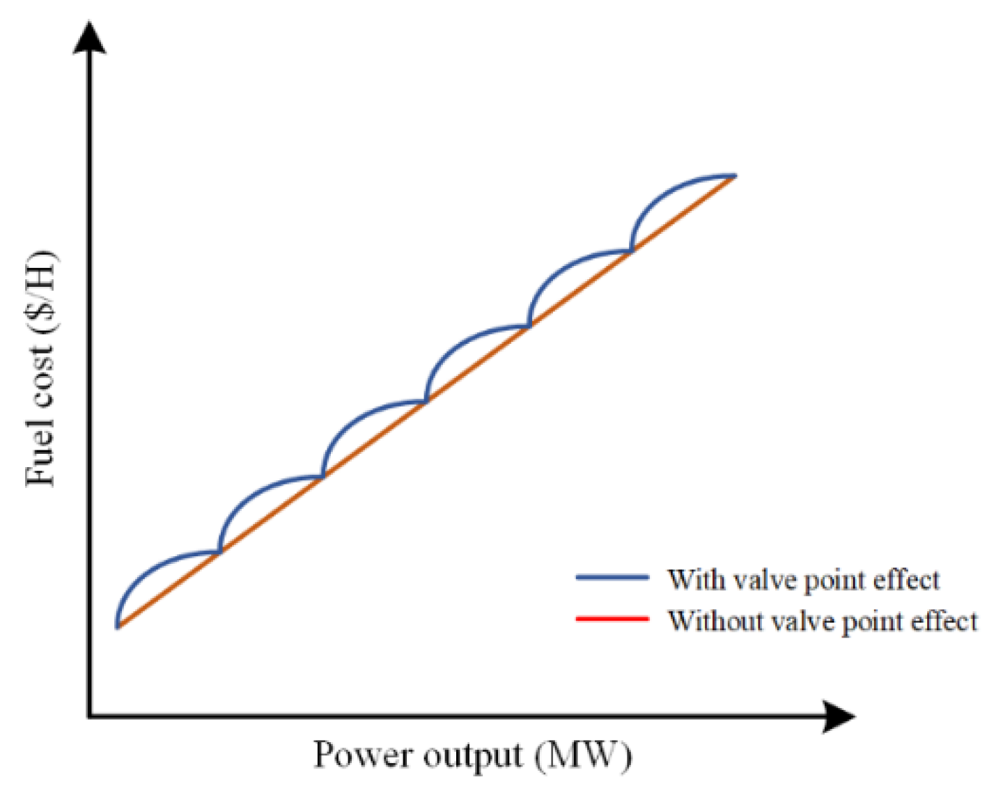
2.1. Objective Function

The objective function of a CHP system includes the generation costs of conventional power-only units, CHP units, and heat-only units, usually represented by Equation (1) [29]:
min f cos t = i = 1 N p C i ( P i p ) + j = 1 N c C j ( P j c , H j c ) + k = 1 N h C k ( H k h )
where P i p and H k h represent the power output of the i -th power-only unit and the heat output of the k -th heat-only unit, respectively; P j c and H j c represent the power and heat outputs of the j -th CHP unit, respectively; Np, Nc, and Nh denote the number of power-only units, CHP units, and heat supply units, respectively; and Ci, Cj, and Ck are the operating costs of the power-only units, CHP units, and heat supply units, respectively and can be expressed is shown in Equations (2)–(4) [30]. Figure 1 is a schematic diagram of the threshold effect.
C i ( P i p ) = α i ( P i p ) 2 + β i P i p + γ i + e e i sin ( f f i ( P i m i n i p ) )
C j ( P j c , H j c ) = a j ( P j c ) 2 + b j P j c + c j + d j ( H j c ) 2 + e j H j c + f j P j c H j c
C k ( H k h ) = φ k ( H k h ) 2 + η k H k h + λ k

2.2. Optimization Constraints

1. The load constraint condition is shown in Equations (5) and (6):
i = 1 N p P i P + j = 1 N c P j c = P D
j = 1 N c H j c + k = 1 N h H k h = H D
In Equations Equations (5) and (6), P D and H D represent the total electrical and thermal energy demands, respectively.
2. Power balance constraint
When considering grid losses, Equation (5) is modified to Equation (7):
i = 1 N p P i p + j = 1 N c P j c = P D + P L
where P L is the grid loss. the mathematical description is shown in Equation (8) [31]:
P L = i = 1 N p m = 1 N p P i m B i m P m p + i = 1 N p j = 1 N c P i p B i j P j c + j = 1 N c n = 1 N c P j c B j n P n c
3. The unit output bounds constraint is shown in Equations (9)–(12):
P i p min P i p P i p max
H k h min H k h H k h max
P j c min ( H j c ) P j c P j c max ( H j c )
H j c min ( P j c ) H j c H j c max ( P j c )
In these equations, P i p max and P i p min are the maximum and minimum power outputs of the i -th power-only unit, H k h max and H k h min are the maximum and minimum heat outputs of the k -th heat supply unit, P j c max ( H j c ) and P j c min ( H j c ) are the maximum and minimum power outputs of the j -th CHP unit, and H j c max ( P j c ) and H j c min ( P j c ) are the maximum and minimum heat outputs of the j -th CHP unit.

2.3. Constraint Repair Technique

In the economic dispatch problem of CHP systems, there are numerous constraints. Therefore, dealing with these constraints effectively is crucial to avoid the local optima.

2.3.1. Equality Constraint Handling

In the CHPED problem, as the algorithm iterates and updates, some solutions may exceed their boundaries and become infeasible. For infeasible solutions, they can be discarded or repaired to become feasible solutions. Here, we use constraint repair to transform these individuals beyond the boundaries into feasible solutions (Figure 2).
1.
For the power-only units, P i p is repaired as in Equation (13):
P i p = P i p min if   P i p P i p min   P i p max if   P i p P i p max P i p o t h e r w i s e
2.
For the heat-only units, H k h is repaired as in Equation (14):
H k h = h k h min if   H k h h k h min h k h max if   H k h h k h max H k h o t h e r w i s e
3.
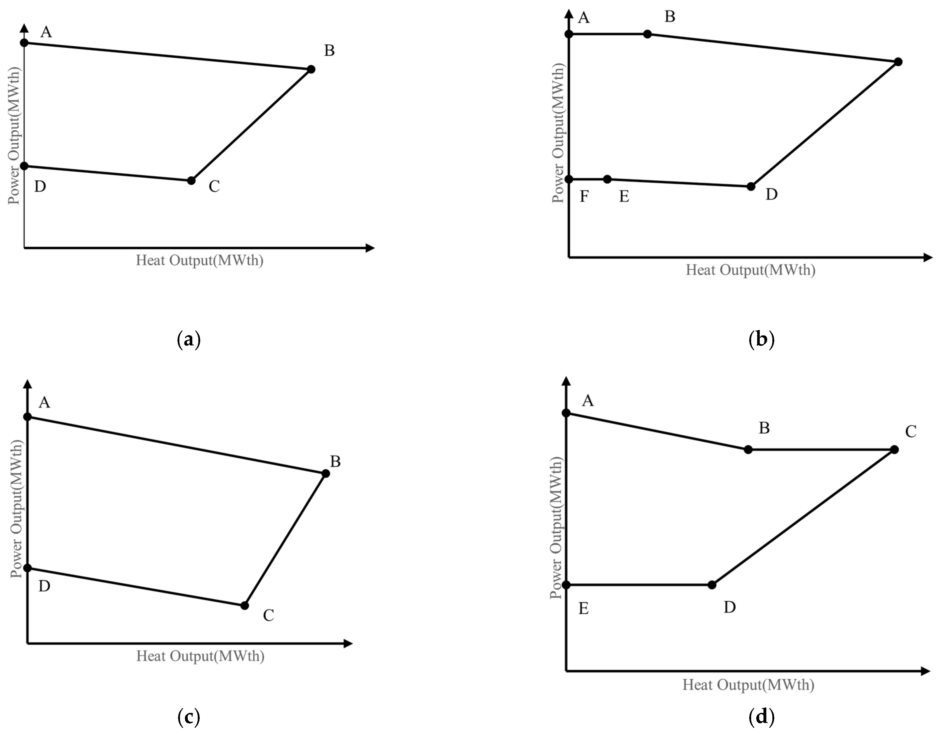
For the CHP units, the power and heat output are interrelated and mutually restricted. P j c min ( H j c ) and P j c max ( H j c ) are calculated based on H j c . Then, P j c is repaired as in Equation (15):
P j c = P j c min ( H j c ) if   P j c P j c min ( H j c ) P j c max ( H j c ) if   P j c P j c max ( H j c ) P j c ( H j c ) o t h e r w i s e
Similarly, H j c min ( P j c ) and H j c max ( P j c ) are calculated based on P j c . Then, H j c is repaired as in Equation (16):
H j c = H j c min ( P j c ) if   H j c H j c min ( P j c ) H j c max ( P j c ) if   H j c H j c max ( P j c ) H j c o t h e r w i s e

2.3.2. Handling of Equality Constraints

1. Total load constraints of the heating and power networks
In the CHPED problem, given the differences in the scale of CHP units, grid losses are often neglected when handling CHPED problems of certain scales. Given that the grid loss values are relatively small for CHP units of specific scales considering grid losses, we assume that these values do not change significantly with fluctuations in unit power when correcting the unit power. Intelligent algorithms are characterized by individual random updates, and thus, when using intelligent algorithms to solve practical problems, it is common to encounter situations where some individuals do not satisfy the equality constraints. This paper adopts the following method to handle equality constraints:
Step 1: Take an individual Xi as a solution and divide Xi into two parts: X i P and X i H . Here, X i P = [P1PNp, P 1 C P N c C ], X i H = [ H 1 C H N c C , H1HNh]. X i H includes the generation from power-only units and CHP units in the system. X i H includes the heating units from heating-only units and the heating components from CHP units in the system. Then, calculate the constraint violation values f p o w e r and f h e a t in Equations (17) and (18):
f p o w e r = P D + P L ( i = 1 N p P i P + j = 1 N c P j c )
f h e a t = H D ( j = 1 N c H j c + k = 1 N h H k h )
Step 2: Repair the power demand constraint. If f p o w e r > 0, select the first variable X i d x P in X i P , and repair X i d x P shown in Equation (19):
X i d x P = min ( X i d x P + f p o w e r , P i d x max )
Step 3: If the value of X i d x P is equal to P i d x max , it indicates that X i d x P + f p o w e r exceeds its boundary. In this case, select the next variable X j d x P , assign the portion of X i d x P + f p o w e r that exceeds the boundary to X j d x P , and use Equation (19) to determine whether X j d x P . exceeds its boundary. Repeat this step until f p o w e r = 0. If, after all variables in X i P have been adjusted, the value of f p o w e r is still not equal to 0, then discard that individual.
Step 4: When f p o w e r < 0, select the first variable X i d x P in X i P , and repair X i d x P shown in Equation (20):
X i d x P = max ( X i d x P f p o w e r , P i d x min )
Step 5: If the value of X i d x P is equal to P i d x min , it indicates that X i d x P f p o w e r exceeds its boundary. In this case, select the next variable X j d x P , assign the portion of X i d x P f p o w e r that exceeds the boundary to X j d x P , and use Equation (20) to determine whether X j d x P exceeds its boundary. Repeat this step until f p o w e r = 0. If, after all variables in X i P have been adjusted, the value of f p o w e r is still not equal to 0, then discard that individual.
Step 6: Repair the heating demand constraint. If f h e a t > 0, select the last variable X i d x H in X i H and perform the following repair X i d x H shown in Equation (21):
X i d x H = min ( X i d x H + f h e a t , H i d x max )
Step 7: If the value of X i d x H is H i d x max , it indicates that the value of X i d x H + f h e a t exceeds its boundary. Choose the previous variable X j d x H and assign the portion of X i d x H + f h e a t that exceeds the boundary to X j d x H . Use Equation (21) to check if X j d x H exceeds its boundary. Repeat this step until f h e a t = 0. If the value of f h e a t still cannot be zero after all variables in X i H have been repaired, discard this individual.
Step 8: When f h e a t < 0, select the last variable X i d x H in X i H and perform the following repair X i d x H shown in Equation (22):
X i d x H = max ( X i d x H f h e a t , H i d x min )
Step 9: If the value of X i d x H is H i d x min , it indicates that the value of X i d x H f h e a t exceeds its boundary. Choose the previous variable X j d x H and assign the portion of X i d x H f h e a t that exceeds the boundary to X j d x H . Use Equation (22) to check if X j d x H exceeds its boundary. Repeat this step until f h e a t = 0. If the value of f h e a t still cannot be zero after all variables in X i H have been repaired, discard this individual.

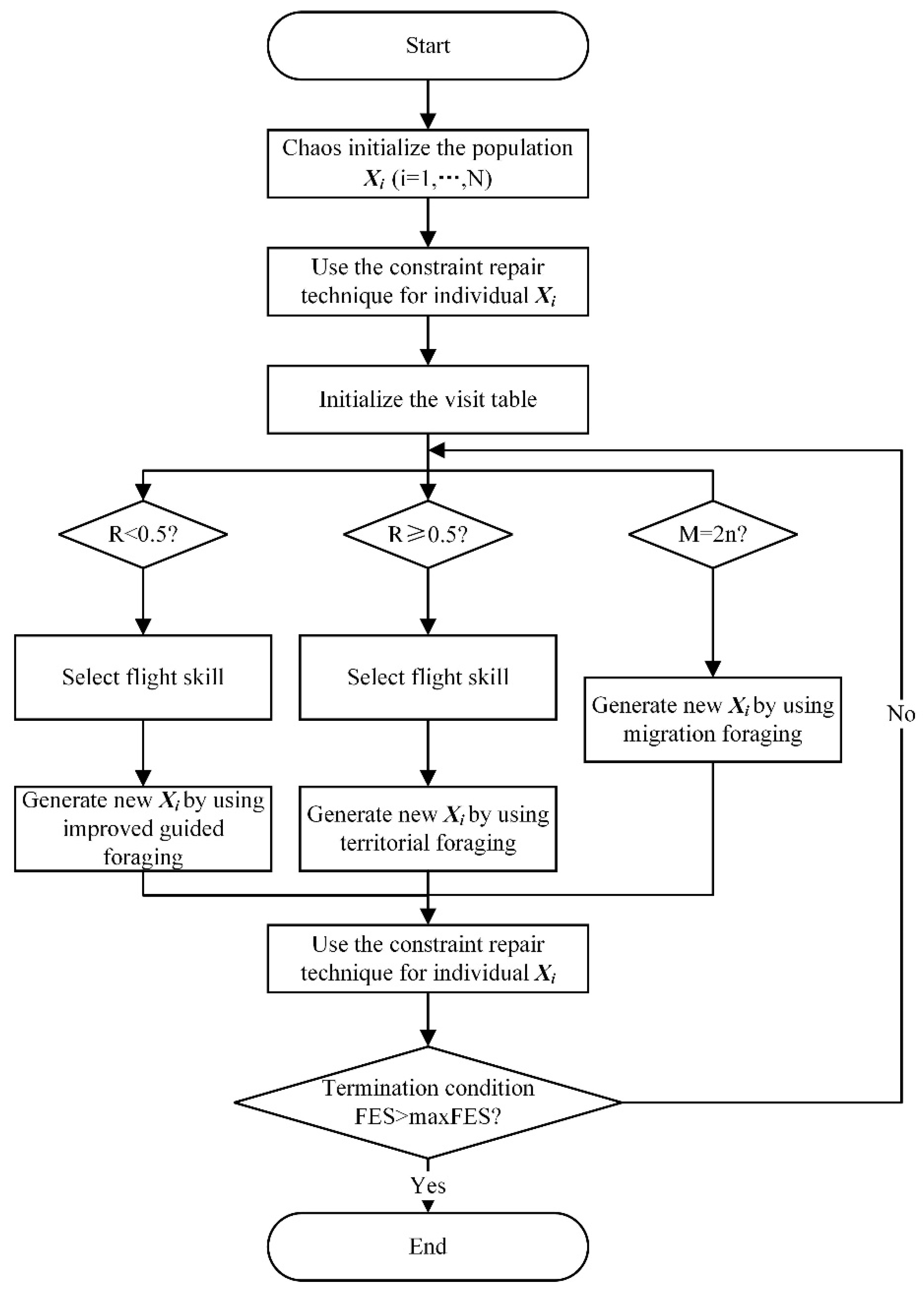
3. Improved Artificial Hummingbird Algorithm

3.1. Introduction of the Artificial Hummingbird Algorithm

The Artificial Hummingbird Algorithm is a novel metaheuristic algorithm proposed by Weiguo Zhao, Liying Wang, and others in 2021 [27]. The algorithm is inspired by the foraging process of hummingbirds for nectar. The basic principle of the algorithm is to use mathematical models to simulate the flight patterns, foraging methods, and memory abilities of hummingbirds during foraging activities.

3.1.1. Flight Patterns

In the AHA, hummingbirds have three types of flight patterns: axial flight, diagonal flight, and omnidirectional flight. These flight patterns are reflected in the algorithm as control over different dimensional directions of the solution space, represented by vector D .
(1) Axial Flight: The hummingbird flies along a specific coordinate axis direction in space. This flight pattern allows the hummingbird to explore in only one dimensional direction. Its mathematical description is shown in Equation (23):
D ( i ) = 1   i f   i   =   r a n d i ( [ 1 , d ] ) 0   else i = 1 , , d
In this context,   r a n d i   ( [ 1 , d ] ) is a random integer between 1 and   d . The 1 in vector D indicates that the hummingbird can fly in the direction of that dimension, meaning the corresponding position in the solution space for that dimension is allowed to be updated.
(2) Diagonal Flight: The hummingbird flies in a diagonal direction formed by randomly chosen coordinate axes. This flight pattern preserves at least one dimension that is not updated. The mathematical description is shown in Equation (24):
D ( i ) = 1 i f i = P ( j ) , j [ 1 , k ] i = 1 , , d 0 e l s e s . t .       P = r a n d p e r m ( k ) k = [ 2 , r 1 ( d 2 ) + 1 ]
R a n d p e r m ( k ) represents a random permutation of integers from 1 to k , and r 1 is a random number within ( 0 , 1 ] . When the value of vector D is 1, it indicates that the hummingbird can update the corresponding position in the solution space for that dimension.
(3) Omnidirectional Flight: The hummingbird flies in directions formed by combinations of all coordinate axes, meaning all dimensions in the solution space are allowed to be updated. The mathematical description is shown in Equation (25):
D ( i ) = 1 i = 1 , . . . , d

3.1.2. Foraging Methods

Hummingbirds have three primary foraging strategies: guided foraging, territorial foraging, and migratory foraging. In the algorithm, these strategies correspond to global search, local search, and mutation search, respectively.
(1) Guided Foraging: In guided foraging, hummingbirds always target the location with the highest unvisited rank as their food source. If there are multiple targets with the same unvisited rank, the one with the highest nectar replenishment rate is chosen. The hummingbird then explores between the target and its current position to find a better food source. Each hummingbird retains a memory of previously visited locations, recording the visit ranks in a visitation table. After each foraging, the unvisited rank of locations that have not been visited increases, while the rank of visited locations drops to the lowest level. The mathematical description of guided foraging is as shown in Equation (26):
v i ( t + 1 ) = x i , t a r ( t ) + a · D · ( x i ( t ) x i , t a r ( t ) )
where t represents number of iterations, a is the guided step size, with a being a value of r a n d , x i , t a r ( t ) is the position of the target food source, and x i ( t ) is the current position of hummingbird i . The position of the i th food source is updated as shown in Equation (27):
x i ( t + 1 ) = x i ( t ) f ( x i ( t ) ) f ( v i ( t + 1 ) ) v i ( t + 1 ) f ( x i ( t ) ) > f ( v i ( t + 1 ) )
When the fitness value f ( x i ( t ) ) of the target food source is better than that of the hummingbird’s current food source (as per Equation (28)), the hummingbird will abandon the current source and move to the new food source.
(2) Territorial Foraging: In territorial foraging, the hummingbird searches for a better food source in the vicinity outside its territory. The mathematical description of territorial foraging is shown in Equation (28):
v i ( t + 1 ) = x i + b · D x i ( t )
where b is the flight step size, with b being a value of r a n d .
(3) Migratory Foraging: After guided or territorial foraging, the hummingbird at the worst food source position needs to migrate to a distant location and quickly find the next food source. The mathematical description of migratory foraging is shown in Equation (29):
x w o r ( t + 1 ) = L o w + r · ( U p L o w )
where x w o r is the food source with the lowest nectar replenishment rate in the population, and U p and L o w are the upper and lower bounds of the solution space, respectively.

3.2. Improving the Artificial Hummingbird Algorithm

Since the CHPED problem considers three types of units simultaneously and involves highly complex constraints, as well as valve point effects and prohibited operating zones, the algorithm used to solve the CHPED problem must have high traversal capability in the solution space and avoid becoming trapped in the local optima. To address the drawbacks of the AHA and solve the CHPED problem more effectively, an IAHA is proposed instead.

3.2.1. Initial Solution

The standard AHA initializes the population using a random initialization method. However, this approach suffers from insufficient traversal and low population diversity, which can negatively impact the convergence speed and optimization accuracy of the AHA. In order to solve these problems, this paper proposes to use chaotic mapping to initialize the population of the algorithm.
Chaos is a complex and widespread phenomenon in nonlinear deterministic systems, reflecting the interaction between order and disorder and between determinism and randomness [32]. Chaotic behavior is confined to a specific region, and its trajectory is complex, unique, and never repeats. Although chaos appears random, it is actually a deterministic system [33].
Chaotic mapping is characterized by randomness, traversal, and regularity. It can traverse the search space non-repetitively within a certain range, according to its own rules. The initial population generated in this way outperforms the traditional random initialization method in terms of solution accuracy and convergence speed, enhancing the population diversity and providing strong adaptability and explorability within the solution space. Therefore, chaotic mapping effectively compensates for the shortcomings of the standard AHA. The mathematical description of chaotic mapping initialization is shown in Equations (30) and (31):
β ( 1 ) = r a n d ( ) β ( i + 1 ) = sin ( π β ( i ) )
X i = β · ( U p L o w ) + L o w
where the strategy is chosen as the chaotic map, and β is the chaotic mapping coefficient. Xi represents the population generated through chaotic mapping.

3.2.2. Modify Update Mechanism

In the standard AHA, whenever the position of a food source is updated, the priority level of the new food sources that have not been visited is usually set to the highest. However, during experiments, it was observed that, if the new food source’s nectar replenishment rate (fitness value) is poor, the hummingbird might fail to utilize the new food source effectively during guided foraging, potentially leading the entire AHA algorithm to become trapped in a local optimum (Figure 3).
To overcome this issue, the original update rule has been modified. Specifically, the priority of the new food source is elevated to the highest level only if its nectar replenishment rate exceeds the average nectar replenishment rate of all the current food sources. Otherwise, the priority levels of the existing food sources remain unchanged. This adjustment not only enhances the algorithm’s convergence speed but also maintains its optimization capability.
The mathematical description of the new update rule is as expressed as Equations (32)–(34):
X i ( n e w F o o d I n d e x ) = x i , n e w + r a n d · D · ( x i x i , n e w )
X i ( o l d F o o d I n d e x ) = x i , o l d + r a n d · D · ( x i x i , n e w )
n e w X i = X i ( n e w F o o d I n d e x ) i f   n e w F i t < i = 1 N F i t / N X i ( o l d F o o d I n d e x ) o t h e r w i s e
where X i ( n e w F o o d I n d e x ) represents the position of the new food source, X i ( o l d F o o d I n d e x ) represents the position of the old food source, x i , n e w represents the position of the target food source, x i , o l d represents the position of the old food source, and xi is the position of the current food source. n e w X i is the new individual generated using the updated rule.

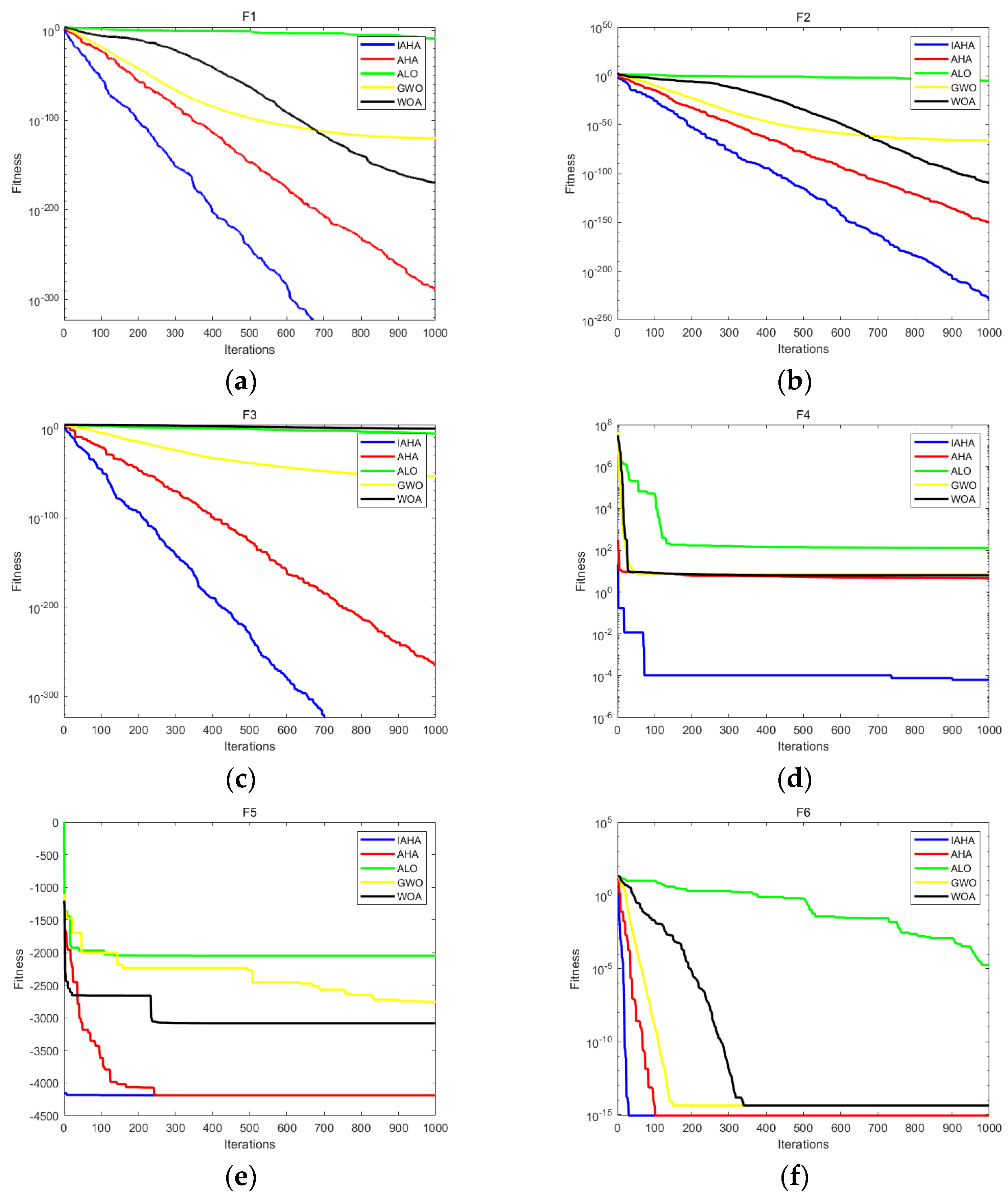
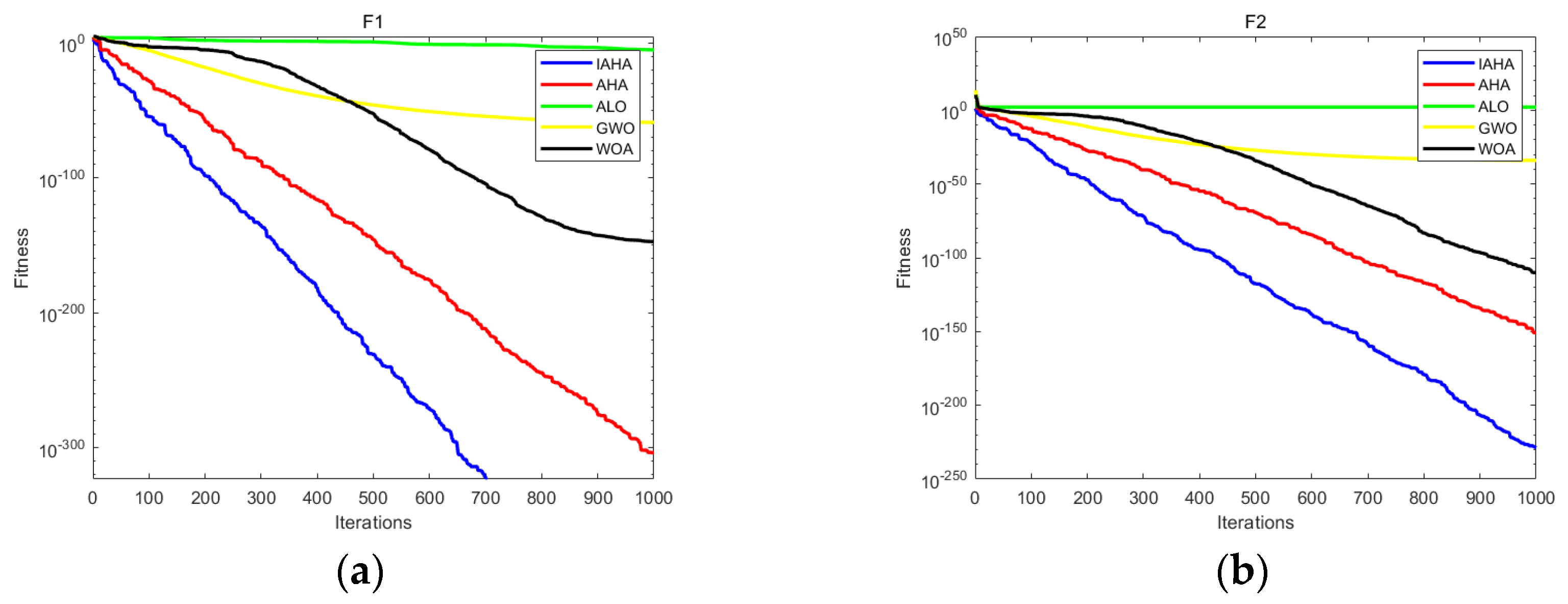
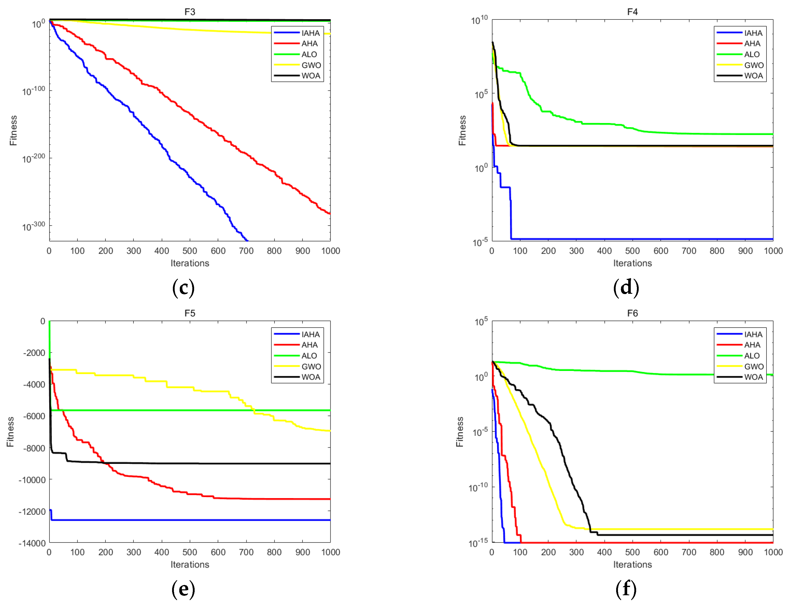
4. Performance Verification of the IAHA

To validate the effectiveness and rationality of the IAHA, it was compared with four other metaheuristic algorithms, which acronyms and parameters are listed in Table 1. The experiments were conducted using six well-known benchmark functions: F1 (Sphere), F2 (Schwefel 2.22), F3 (Schwefel 1.2), F4 (Rosenbrock), F5 (Schwefel), and F6 (Ackley), selected from the 23 benchmark test functions mentioned in the literature [34]. These experiments demonstrated the effectiveness and superiority of the IAHA. As shown in Table 1, the selected benchmark functions include both unimodal and multimodal test functions. Unimodal functions have only one global optimum, making it easy to determine, whereas multimodal functions have multiple local optima, making it difficult to find the global optimum. Therefore, the chosen benchmark functions can effectively evaluate the algorithm’s performance in escaping the local optima and convergence speed. To verify the robustness of IAHA across different dimensions of the same test function, the algorithm’s ability was tested using dimensions of 10, 30, and 50 for both unimodal and multimodal test functions, and each dimension was tested separately 30 times. The maximum number of iterations was uniformly set to 1000. When the evaluation times of the function reach the maximum number of iterations, the optimization process of the algorithm will stop. All experiments in this study were conducted on a PC equipped with a 12th Gen Intel(R) Core (TM) i7-12700H 2.30 GHz processor and 16 GB of RAM. Table 1 shows the names and abbreviations of five algorithms. Table 2 shows the parameter settings and iteration of five algorithms Table 3 shows the names and parameters of six test functions. The experimental results are shown in Table 4, Table 5 and Table 6. In Figure 4, Figure 5 and Figure 6, subgraphs a-f show the iterative curves of different algorithms on the test function F1–6

5. Experimental Results

In this section, the IAHA algorithm is applied to solve the CHPED problem, and three systems of different sizes are adopted. To verify its effectiveness, we compared the IAHA with various other algorithms across different test systems.

5.1. Population Coding

In the CHPED problem, each individual is composed of the power and heat outputs from power-only units, CHP units, and heat-only units. When the AHA is employed to solve the CHPED problem, the solution matrix of the algorithm consists of two parts: the number of individuals and the number of units. Here, the number of solutions is equivalent to the number of hummingbirds in the AHA, and the number of units corresponds to the dimensions in the AHA. To better represent these two sub-problems, this paper encodes individuals in the following manner as Equation (35):
X = P 11 p P 1 N p p , P 11 c P 1 N c c , H 11 c H 1 N c c , H 11 h H 1 N h h P 21 p P 2 N p p , P 21 c P 2 N c c , H 21 c H 2 N c c , H 21 h H 2 N h h P N 1 p P N N p p , P N 1 c P N N c c , H N 1 c H N N c c , H N 1 h H N N h h
where X is the population matrix, and N is the number of individuals. P 11 p represents the power output of the first power-only unit in the first individual, while P 1 N p p represents the power output of the last power-only unit in the first individual. P 11 c denotes the power output of the first CHP unit in the first individual, and P 1 N c c represents the power output of the last CHP unit in the first individual. H 11 c stands for the heat output of the first CHP unit in the first individual, and H 1 N c c represents the heat output of the last CHP unit in the first individual. H 11 h is the heat output of the first heat-only unit in the first individual, and H 1 N h h represents the heat output of the last heat-only unit in the first individual.
Similarly, P N 1 p is the power output of the first power-only unit in the last individual, and P N N p p is the power output of the last power-only unit in the last individual. P N 1 c is the power output of the first CHP unit in the last individual, and P N N c c is the power output of the last CHP unit in the last individual. H N 1 c is the heat output of the first CHP unit in the last individual, and H N N c c is the heat output of the last CHP unit in the last individual. H N 1 h is the heat output of the first heat-only unit in the last individual, and H N N h h is the heat output of the last heat-only unit in the last individual (Figure 7).

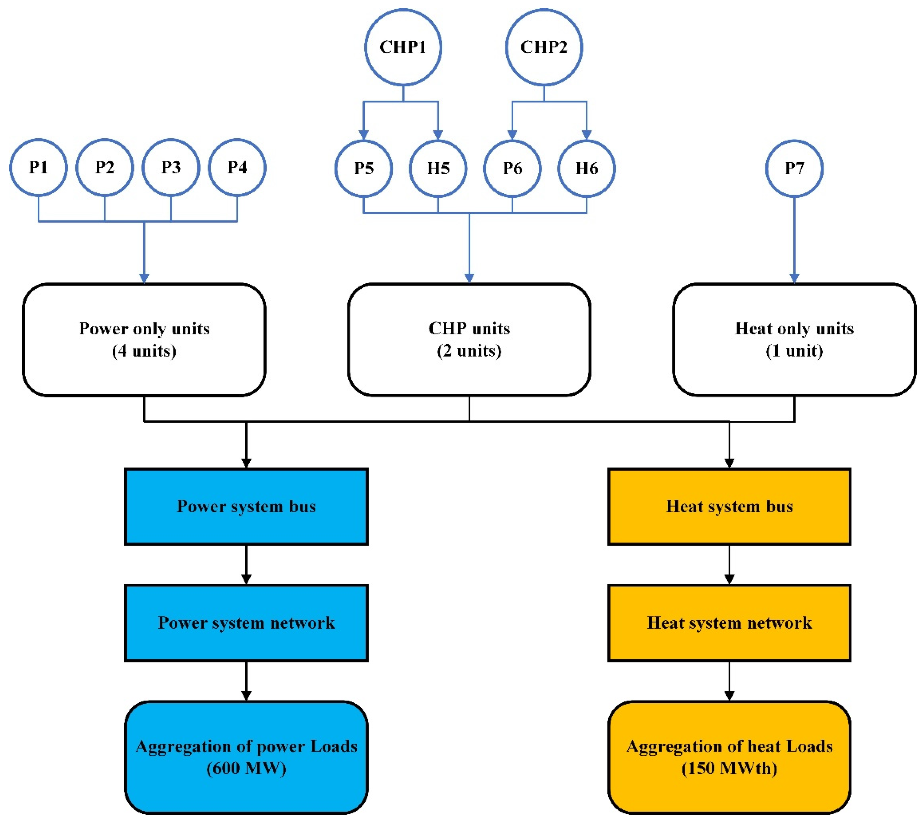
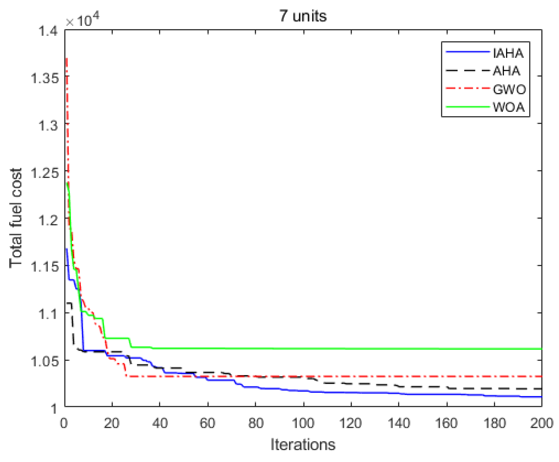
5.2. Test System 1: 7-Unit CHPED Problem

The first test system is a seven-unit CHPED problem, taken from reference [37]. It is a classic small-scale CHPED problem consisting of four power-only units, two CHP units, and one heat-only unit. In Test System 1, grid losses, valve point effects, and operational regions were considered. The maximum number of iterations was set to MaxIt = 1000, and the population size NP = 100. Accordingly, Table 7, Table 8 and Table 9 list the relevant parameters of the operational cost functions for each unit. The data were sourced from [38].
The grid loss coefficient is provided by Equation (36) [24]:
B = 49 14 15 15 20 25 14 45 16 20 18 19 15 16 39 10 12 15 15 20 10 40 14 11 20 18 12 14 35 17 25 19 15 11 17 39 × 10 7
According to Reference [37], the power load of Test System 1 is 600 MW, and the thermal load (Hp) is 150 MWth.
Table 10 lists the optimal, average, and worst costs, as well as the running time, of various algorithms in four experiments: IAHA, AHA, GWO, and WOA. Additionally, Table 10 also compares the results from HTS [18], BLPSO [39], ISNS [40], and Levy-GWO [24] in the literature.
From Table 10 and Table 11, it can be seen that, compared to all algorithms in experiments and the literature, IAHA has achieved the best results in terms of optimal, average, and worst costs. The optimal cost obtained by IAHA is only USD 10,093.75, which is lower than the optimal values obtained by other algorithms in Table 10. Compared to the WOA in the experiment, IAHA achieved the best cost savings of up to USD 232.65. Compared to the Levy-GWO in the literature [24], IAHA achieves an optimal cost savings of up to USD 18.04. Considering the average cost, IAHA also obtained a smaller value (i.e., USD 10,093.76), indicating that IAHA also has good stability.
From Table 11, it can be seen that the power output of each unit obtained by IAHA is more stable, with few cases where the power output is at the power boundary. This is mainly due to AHA’s unique flying, foraging, and memory abilities, which can quickly and accurately find the optimal solution. Meanwhile, IAHA is slightly inferior to AHA in terms of algorithm runtime. This is because, compared to AHA, IAHA’s search space is more extensive, but at the same time, it enhances the population diversity of the algorithm and the ability to jump out of the local optimum.
The convergence processes of the four algorithms are shown in Figure 8. From Figure 8, it can be seen that the convergence speed and accuracy of the IAHA are higher than those of the other algorithms shown. The electrical and thermal energy values obtained by the IAHA algorithm are very close to the required power loads.

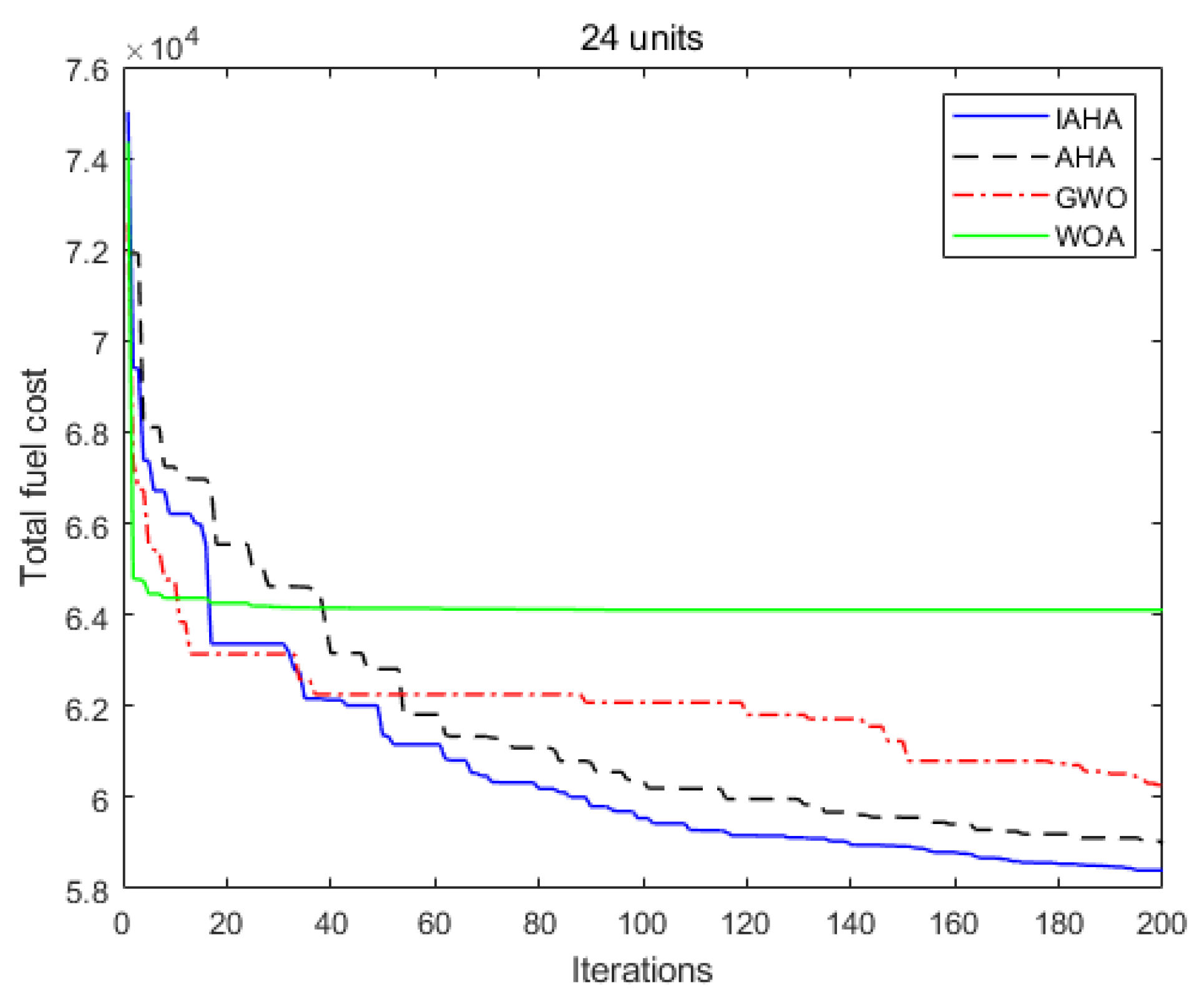
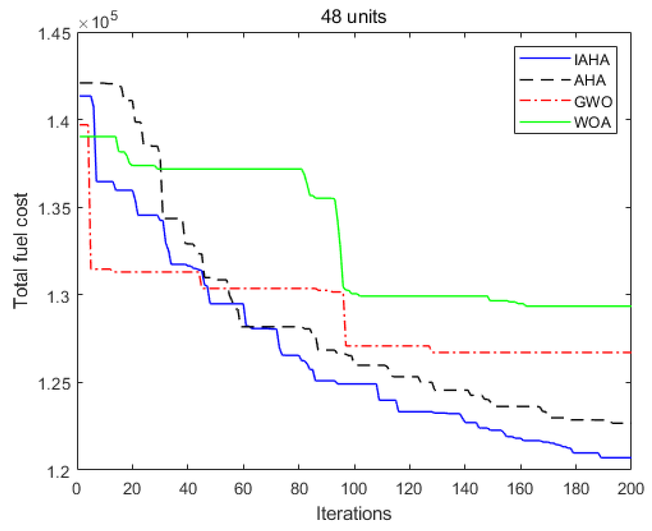
5.3. Test System 2: 24-Unit CHPED Problem

Test System 2 is a 24-unit CHPED problem, taken from Reference [41]. It is a classic medium-scale CHPED problem consisting of 13 power-only units, 6 CHP units, and 5 heat-only units. In Test System 2, valve point effects and operational regions were considered. The maximum number of iterations was set to MaxIt = 4000, and the population size NP = 150. Accordingly, Table 12, Table 13 and Table 14 list the relevant parameters of the operational cost functions for each unit. The data are sourced from [38].
According to Reference [41], the power load of Test System 2 is 2350 MW, and the thermal load (Hp) is 1250 MWth.
Table 15 lists the optimal, average, and worst costs, as well as the running time, of various algorithms in four experiments: IAHA, AHA, GWO, and WOA. In addition, Table 15 also compares the results from the proposed CHPED algorithm [6], HTS [18], ISNS [40], and SNS [40] in the literature.
From Table 15 and Table 16, it can be seen that, compared to all algorithms in the experiment and literature, IAHA has obtained the best results in terms of the optimal, average, and worst costs. The optimal cost obtained by IAHA is only USD 57,876.5508, which is lower than the optimal values obtained by other algorithms in Table 15. Compared to the WOA in the experiment, IAHA achieved the best cost savings of up to USD 4006.6307. Compared to the SNS in the literature [40], IAHA achieves the best cost savings of up to USD 232.7894. Considering the average cost, IAHA also obtained a smaller value (i.e., 57,894.9375), indicating that IAHA also has good stability.
From Table 16, it can be seen that the power output of each unit obtained by IAHA is more stable, with few cases where the power output is at the power boundary. In terms of algorithm run time, IAHA shows a significant advantage over other algorithms, primarily due to the unique memory capability of AHA. Each hummingbird retains a memory of positions with higher nectar replenishment rates during iterations, which significantly reduces the algorithm’s run time.
As shown in Figure 9, compared to the other three algorithms, both the convergence speed and accuracy of IAHA are improved.
Test Case 3 is a 48-unit CHPED problem taken from Reference [41]. It is a classic large-scale CHPED problem consisting of 26 power-only units, 12 CHP units, and 10 heat-only units. In Test System 3, valve point effects and operational regions were considered. The maximum number of iterations is set to MaxIt = 20,000, and the population size NP = 200. Accordingly, Table 17, Table 18 and Table 19 list the relevant parameters of the operational cost functions for each unit. The data are sourced from [41].
According to Reference [5], the power load of Test System 3 is 4700 MW, and the thermal load (Hp) is 2500 MWth.
Table 20 lists the optimal, average, and worst costs, as well as the running time, of various algorithms in four experiments: IAHA, AHA, GWO, and WOA. In addition, Table 20 also compares the results from HTS [18], ISNS [40], SNS [40], and HBJSA [42] in the literature.
From Table 20 and Table 21, it can be seen that, compared to all algorithms in the experiments and literature, IAHA has achieved the best results in terms of the optimal, average, and worst costs. The optimal cost obtained by IAHA is only USD 116,048.1539, which is lower than the optimal values obtained by other algorithms in Table 20. Compared to the WOA in the experiment, IAHA achieved the best cost savings of up to USD 13,997.7473. Compared to the SNS in the literature [40], IAHA achieves the best cost savings of up to USD 870.7461. Considering the average cost, IAHA also obtained a smaller value (i.e., 116,111.1857), indicating that IAHA also has good stability.
From Table 21, it can be seen that the power output of each unit obtained by IAHA is more stable, with few cases where the power output is at the power boundary. Additionally, due to AHA’s unique access table mechanism and memory capability, both IAHA and AHA have significant advantages in processing large-scale CHPED problems in terms of run time.
As shown in Figure 10, both the convergence speed and accuracy of IAHA are superior to the other three algorithms.

6. Summary

This paper introduces an Improved Artificial Hummingbird Algorithm (abbreviated as IAHA) designed to address complex CHPED problems more effectively. The algorithm employs chaotic mapping for population initialization, enhances the iterative mechanism of the original IAHA, boosts the algorithm’s traversal capability and population diversity, overcomes its shortcomings, and mitigates the risk of premature convergence. We evaluated the performance of IAHA using benchmark test functions and compared it with several other commonly used algorithms. The results demonstrate that IAHA can discover high-quality solutions within a relatively short period. Furthermore, simulation experiments were conducted on three CHPED using IAHA, with the test units including 7 units, 24 units, and 48 units, respectively. The results indicate that IAHA is capable of generating optimal solutions, confirming its effectiveness in solving CHPED problems.
However, there are also some limitations in this study. Firstly, due to the enhanced traversal capability of IAHA based on the original AHA, the exploration space for hummingbirds expands, resulting in a slight decrease in computational speed. Additionally, more factors have not been taken into account when solving the CHPED problem. In the future, we plan to incorporate factors such as dynamic economic dispatch and environmental pollution into the CHPED framework, which will help in addressing real-world challenges.

Author Contributions

X.K.: Conceptualization, Software, Investigation, Formal analysis, Validation, Visualization, and Writing—Original Draft; K.L.: Methodology, Software, Data curation, Validation, Visualization, and Writing—Original Draft; Y.Z.: Validation, Formal analysis, and Investigation; G.T.: Validation, Formal analysis, and Investigation; N.D.: Validation, Formal analysis, and Investigation. All authors have read and agreed to the published version of the manuscript.

Funding

The Scientific and Technological Project of Henan Province (No. 222102110095).

Data Availability Statement

The original contributions presented in the study are included in the article, further inquiries can be directed to the corresponding author.

Conflicts of Interest

The authors declare no conflicts of interest.

References

  1. Yang, W.; Zhang, Y.; Zhu, X.; Li, K.; Yang, Z. Research on Dynamic Economic Dispatch Optimization Problem Based on Improved Grey Wolf Algorithm. Energies 2024, 17, 1491. [Google Scholar] [CrossRef]
  2. Li, D.; Yang, C. A Modified Genetic Algorithm for Combined Heat and Power Economic Dispatch. J. Bionic Eng. 2024, 21, 2569–2586. [Google Scholar] [CrossRef]
  3. Wang, S.K.; Zhang, L.; Liu, C.; Liu, Z.M.; Lan, S.; Li, Q.B.; Wang, X.N. Techno-economic-environmental evaluation of a combined cooling heating and power system for gas turbine waste heat recovery. Energy 2021, 231, 15. [Google Scholar] [CrossRef]
  4. Xiao, T.Y.; Liu, C.; Wang, X.R.; Wang, S.K.; Xu, X.X.; Li, Q.B.; Li, X.X. Life cycle assessment of the solar thermal power plant integrated with air-cooled supercritical CO2 Brayton cycle. Renew. Energy 2022, 182, 15. [Google Scholar] [CrossRef]
  5. Chen, X.; Shen, A. Self-adaptive differential evolution with Gaussian–Cauchy mutation for large-scale CHP economic dispatch problem. Neural Comput. Appl. 2022, 34, 11769–11787. [Google Scholar] [CrossRef]
  6. Kaur, P.; Chaturvedi, K.T.; Kolhe, M.L. Techno-Economic Power Dispatching of Combined Heat and Power Plant Considering Prohibited Operating Zones and Valve Point Loading. Processes 2022, 10, 817. [Google Scholar] [CrossRef]
  7. Miller, T.; Durlik, I.; Kostecka, E.; Kozlovska, P.; Jakubowski, A.; Łobodzińska, A. Waste Heat Utilization in Marine Energy Systems for Enhanced Efficiency. Energies 2024, 17, 5653. [Google Scholar] [CrossRef]
  8. Jadoun, V.K.; Prashanth, G.R.; Joshi, S.S.; Agarwal, A.; Almutairi, A. Optimal Scheduling of Non-Convex Cogeneration Units Using Exponentially Varying Whale Optimization Algorithm. Energies 2021, 14, 1008. [Google Scholar] [CrossRef]
  9. Zou, D.; Ma, L.; Li, C. An enhanced NSGA-II and a fast constraint repairing method for combined heat and power dynamic economic emission dispatch. Inf. Sci. 2024, 678, 120915. [Google Scholar] [CrossRef]
  10. Wong, K.P.; Algie, C. Evolutionary programming approach for combined heat and power dispatch. Electr. Power Syst. Res. 2002, 61, 227–232. [Google Scholar] [CrossRef]
  11. Rooijers, F.J.; Van Amerongen, R.A.M. Static economic dispatch for co-generation systems. Power Syst. IEEE Trans. 1994, 9, 1392–1398. [Google Scholar] [CrossRef]
  12. Haghrah, A.; Nekoui, M.; Nazari-Heris, M.; Mohammadi-Ivatloo, B. An improved real-coded genetic algorithm with random walk based mutation for solving combined heat and power economic dispatch. J. Ambient Intell. Humaniz. Comput. 2021, 12, 8561–8584. [Google Scholar] [CrossRef]
  13. Liu, D.; Hu, Z.; Su, Q.; Liu, M. A niching differential evolution algorithm for the large-scale combined heat and power economic dispatch problem. Appl. Soft Comput. 2021, 113, 108017. [Google Scholar] [CrossRef]
  14. Shaheen, A.M.; Elsayed, A.M.; Ginidi, A.R.; El-Sehiemy, R.A.; Ghoneim, S.S.M. A novel improved marine predators algorithm for combined heat and power economic dispatch problem. AEJ-Alex. Eng. J. 2021, 61, 1834–1851. [Google Scholar] [CrossRef]
  15. Ramachandran, M.; Mirjalili, S.; Ramalingam, M.M.; Gnanakkan, C.A.R.C.; Parvathysankar, D.S.; Sundaram, A. A ranking-based fuzzy adaptive hybrid crow search algorithm for combined heat and power economic dispatch. Expert Syst. Appl. 2022, 197, 116625. [Google Scholar] [CrossRef]
  16. Sun, J.; Deng, J.; Li, Y. Indicator & crowding Distance-Based Evolutionary Algorithm for Combined Heat and Power Economic Emission Dispatch. arXiv 2020, arXiv:2002.11513. [Google Scholar]
  17. Zhou, T.; Chen, J.; Xu, X.; Ou, Z.; Yin, H.; Luo, J.; Meng, A. A novel multi-agent based crisscross algorithm with hybrid neighboring topology for combined heat and power economic dispatch. Appl. Energy 2023, 342, 121167. [Google Scholar] [CrossRef]
  18. Pattanaik, J.K.; Basu, M.; Dash, D.P. Heat transfer search algorithm for combined heat and power economic dispatch. Iran. J. Sci. Technol. Trans. Electr. Eng. 2020, 44, 963–978. [Google Scholar] [CrossRef]
  19. Ozkaya, B.; Duman, S.; Kahraman, H.T.; Guvenc, U. Optimal solution of the combined heat and power economic dispatch problem by adaptive fitness-distance balance based artificial rabbits optimization algorithm. Expert Syst. Appl. 2024, 238, 122272. [Google Scholar] [CrossRef]
  20. Nazari-Heris, M.; Mohammadi-Ivatloo, B.; Asadi, S.; Geem, Z.W. Large-Scale Combined Heat and Power Economic Dispatch Using a Novel Multi-Player Harmony Search Method. Appl. Therm. Eng. 2019, 154, 493–504. [Google Scholar] [CrossRef]
  21. Huang, Z.; Gao, Z.; Qi, L.; Duan, H. A Heterogeneous Evolving Cuckoo Search Algorithm for Solving Large-scale Combined Heat and Power Economic Dispatch Problems. IEEE Access 2019, 7, 111287–111301. [Google Scholar] [CrossRef]
  22. Rabiee, A.; Jamadi, M.; Mohammadi-Ivatloo, B.; Ahmadian, A. Optimal Non-Convex Combined Heat and Power Economic Dispatch via Improved Artificial Bee Colony Algorithm. Processes 2020, 8, 1036. [Google Scholar] [CrossRef]
  23. Spea, S.R. Social network search algorithm for combined heat and power economic dispatch. Electr. Power Syst. Res. 2023, 221, 109400. [Google Scholar] [CrossRef]
  24. Wang, Y.; Yu, X.B.; Yang, L.; Li, J.; Zhang, J.; Liu, Y.L.; Sun, Y.J.; Yan, F. Research on Load Optimal Dispatch for High-Temperature CHP Plants through Grey Wolf Optimization Algorithm with the Levy Flight. Processes 2022, 10, 1546. [Google Scholar] [CrossRef]
  25. Wolpert, D.H.; Macready, W.G. No free lunch theorems for optimization. IEEE Trans. Evol. Comput. 1997, 1, 67–82. [Google Scholar] [CrossRef]
  26. Ramachandran, M.; Mirjalili, S.; Nazari-Heris, M.; Parvathysankar, D.S.; Sundaram, A.; Gnanakkan, C. A hybrid Grasshopper Optimization Algorithm and Harris Hawks Optimizer for Combined Heat and Power Economic Dispatch problem. Eng. Appl. Artif. Intell. 2022, 111, 39. [Google Scholar] [CrossRef]
  27. Zhao, W.G.; Wang, L.Y.; Mirjalili, S. Artificial hummingbird algorithm: A new bio-inspired optimizer with its engineering applications. Comput. Meth. Appl. Mech. Eng. 2022, 388, 45. [Google Scholar] [CrossRef]
  28. Kansal, V.; Dhillon, J.S.; Yan, J. Ameliorated artificial hummingbird algorithm for coordinated wind-solar-thermal generation scheduling problem in multiobjective framework. Appl. Energy 2022, 326, 120031. [Google Scholar] [CrossRef]
  29. Ozkaya, B.; Kahraman, H.T.; Duman, S.; Guvenc, U.; Akbel, M. Combined heat and power economic emission dispatch using dynamic switched crowding based multi-objective symbiotic organism search algorithm. Appl. Soft Comput. 2024, 151, 111106. [Google Scholar] [CrossRef]
  30. Chen, X.; Fang, S.; Li, K. Reinforcement-Learning-Based Multi-Objective Differential Evolution Algorithm for Large-Scale Combined Heat and Power Economic Emission Dispatch. Energies 2023, 16, 3753. [Google Scholar] [CrossRef]
  31. Mekhamer, S.; Abdelaziz, A.; Badr, M.; Kamh, M. Enhancing the performance of Hopfield neural network applied to the economic dispatch problem. In Proceedings of the 2006 Eleventh International Middle East Power Systems Conference, El-Minia, Egypt, 19–21 December 2006; pp. 347–352. [Google Scholar]
  32. Yin, L.; Sun, Z. Multi-layer distributed multi-objective consensus algorithm for multi-objective economic dispatch of large-scale multi-area interconnected power systems. Appl. Energy 2021, 300, 117391. [Google Scholar] [CrossRef]
  33. Yang, W.; Zhu, X.; Nie, F.; Jiao, H.; Xiao, Q.; Yang, Z. Chaos Moth Flame Algorithm for Multi-Objective Dynamic Economic Dispatch Integrating with Plug-In Electric Vehicles. Electronics 2023, 12, 2742. [Google Scholar] [CrossRef]
  34. Mirjalili, S.; Mirjalili, S.M.; Lewis, A. Grey wolf optimizer. Adv. Eng. Softw. 2014, 69, 46–61. [Google Scholar] [CrossRef]
  35. Mirjalili, S. The ant lion optimizer. Adv. Eng. Softw. 2015, 83, 80–98. [Google Scholar] [CrossRef]
  36. Mirjalili, S.; Lewis, A. The whale optimization algorithm. Adv. Eng. Softw. 2016, 95, 51–67. [Google Scholar] [CrossRef]
  37. Basu, M. Combined Heat and Power Economic Dispatch by Using Differential Evolution. Electr. Power Compon. Syst. 2010, 38, 996–1004. [Google Scholar] [CrossRef]
  38. Mohammadi-Ivatloo, B.; Moradi-Dalvand, M.; Rabiee, A. Combined heat and power economic dispatch problem solution using particle swarm optimization with time varying acceleration coefficients. Electr. Power Syst. Res. 2013, 95, 9–18. [Google Scholar] [CrossRef]
  39. Chen, X.; Li, K.; Xu, B.; Yang, Z. Biogeography-based learning particle swarm optimization for combined heat and power economic dispatch problem. Knowl.-Based Syst. 2020, 208, 106463. [Google Scholar] [CrossRef]
  40. Gafar, M.; Ginidi, A.; El-Sehiemy, R.; Sarhan, S. Improved SNS algorithm with high exploitative strategy for dynamic combined heat and power dispatch in co-generation systems. Energy Rep. 2022, 8, 8857–8873. [Google Scholar] [CrossRef]
  41. Zou, D.; Li, S.; Kong, X.; Ouyang, H.; Li, Z. Solving the combined heat and power economic dispatch problems by an improved genetic algorithm and a new constraint handling strategy. Appl. Energy 2019, 237, 646–670. [Google Scholar] [CrossRef]
  42. Ginidi, A.; Elsayed, A.; Shaheen, A.; Elattar, E.; El-Sehiemy, R. An Innovative Hybrid Heap-Based and Jellyfish Search Algorithm for Combined Heat and Power Economic Dispatch in Electrical Grids. Mathematics 2021, 9, 2053. [Google Scholar] [CrossRef]
Figure 1. Schematic diagram of the threshold effect.
Energies 17 06411 g001
Figure 2. Operable region of the units. (a) Suitable operation area for the Type A cogeneration unit. (b) Suitable operation area for the Type B cogeneration unit. (c) Suitable operation area for the Type C cogeneration unit. (d) Suitable operation area for the Type D cogeneration unit.
Energies 17 06411 g002
Figure 3. Flowchart of the IAHA.
Energies 17 06411 g003
Figure 4. Convergence comparison curves of various algorithms (10 dimensions). (af) show the convergence curves of various algorithms on test functions 1–6.
Energies 17 06411 g004
Figure 5. Convergence comparison curves of various algorithms (30 dimensions). (af) show the convergence curves of various algorithms on test functions 1–6.
Energies 17 06411 g005aEnergies 17 06411 g005b
Figure 6. Convergence comparison curves of various algorithms (50 dimensions). (af) show the convergence curves of various algorithms on test functions 1–6.
Energies 17 06411 g006
Figure 7. A single line diagram of the CHP economic dispatch problem considering the 7-unit test system.
Energies 17 06411 g007
Figure 8. Comparison of the convergence curves of 4 algorithms in test system 1.
Energies 17 06411 g008
Figure 9. Comparison of the convergence curves of 4 algorithms in test system 2.5.4. Test System 3: 48-Unit CHPED Problem.
Energies 17 06411 g009
Figure 10. Comparison of the convergence curves of 4 algorithms in test system 3.
Energies 17 06411 g010
Table 1. List of algorithm abbreviations.
Table of AbbreviationsAbbreviations
1. Artificial Hummingbird AlgorithmAHA [27]
2. Ant Lion OptimizerALO [35]
3. Grey Wolf OptimizerGWO [34]
4. Whale Optimization AlgorithmWOA [36]
5. Improved Artificial Hummingbird AlgorithmIAHA
Table 2. Algorithm parameters table.
AlgorithmsParameter SettingsIteration
Artificial Hummingbird AlgorithmNP = 301000
Ant Lion OptimizerNP = 301000
Grey Wolf OptimizerNP = 301000
Whale Optimization AlgorithmNP = 30, b = 11000
Improved Artificial Hummingbird AlgorithmNP = 301000
Table 3. Basic test functions.
Function NameDimRangeFmin
Sphere10/30/50[−100, 100]0
Schwefel 2.2210/30/50[−10, 10]0
Schwefel 1.210/30/50[−100, 100]0
Rosenbrock10/30/50[−30, 30]0
Schwefel10/30/50[−500, 500]−12,569.5
Ackley10/30/50[−32, 32]0
Table 4. Comparison of the IAHA with other algorithms (10 dimensions).
NO.StatisticsALOGWOWOAAHAIAHA
F1Mean2.67 × 10−94.07 × 10−1171.02 × 10−1572.12 × 10−2770.00
Sta1.16 × 10−91.99 × 10−1164.69 × 10−1570.000.00
Best1.09 × 10−91.08 × 10−1238.64 × 10−1741.02 × 10−3100.00
Time (s)160.24160.28160.33155.18155.24
Winner1111
F2Mean2.69 × 10−12.98 × 10−671.49 × 10−1064.24 × 10−1443.25 × 10−226
Sta7.77 × 10−14.99 × 10−676.20 × 10−1061.56 × 10−1430.00
Best6.57 × 10−61.78 × 10−699.19 × 10−1061.13 × 10−1541.74 × 10−242
Time (s)158.32158.37158.42153.29153.35
Winner1111
F3Mean9.38 × 10−65.46 × 10−522.35 × 1011.73 × 10−2440.00
Sta1.05 × 10−52.03 × 10−518.07 × 1010.000.00
Best1.09 × 10−71.10 × 10−643.56 × 10−101.70 × 10−2780.00
Time (s)163.46163.56163.66158.39158.49
Winner1111
F4Mean5.21 × 10−10.65 × 1010.62 × 1010.45 × 1011.87 × 10−4
Sta1.04 × 1020.09 × 1010.04 × 1010.04 × 1016.58 × 10−4
Best5.15 × 10−40.47 × 1010.55 × 1010.34 × 1014.4 × 10−7
Time (s)159.53159.59159.66154.44154.50
Winner1111
F5Mean−2.47 × 10³−2.71 × 10³−3.37 × 10³−4.19 × 10³−4.19 × 10³
Sta6.42 × 10−22.96 × 10−26.06 × 10−22.80 × 10−73.13 × 10−3
Best−4.19 × 10³−3.23 × 10³−4.19 × 10³−4.19 × 10³−4.19 × 10³
Time (s)157.85157.91157.99152.83152.89
Winner111−1
F6Mean1.60 × 10−14.67 × 10−154.09 × 10−158.88 × 10−168.88 × 10⁻¹⁶
Sta5.03 × 10−19.01 × 10−162.16 × 10−150.000.00
Best1.50 × 10−54.44 × 10−158.88 × 10−168.88 × 10−168.88 × 10⁻¹⁶
Time (s)344.87344.92344.98339.82339.87
Winner111−1
Table 5. Comparison of the IAHA with other algorithms (30 dimensions).
NO.StatisticsALOGWOWOAAHAIAHA
F1Mean1.02 × 10−56.40 × 10−592.16 × 10−1493.05 × 10−2840.00
Sta7.63 × 10−61.37 × 10−581.04 × 10−1480.000.00
Best1.16 × 10−62.20 × 10−627.01 × 10−1691.54 × 10−3150.00
Time (s)663.6472663.7312663.7962647.4758649.5391
Winner1111
F2Mean4.34 × 1017.84 × 10−358.90 × 10−1045.01 × 10−1481.05 × 10−224
Sta5.26 × 1014.84 × 10−354.51 × 10−1031.71 × 10−1470.00
Best1.99 × 10−24.96 × 10−361.06 × 10−1121.06 × 10−1623.71 × 10−245
Time (s)520.2035520.2883520.3485506.1642506.2296
Winner1111
F3Mean1.09 × 1035.24 × 10−152.07 × 1042.00 × 10−2640.00
Sta6.43 × 1021.47 × 10−149.64 × 1030.000.00
Best3.89 × 1021.01 × 10−203.30 × 1035.68 × 10−3010.00
Time (s)456.5424456.7693456.9743442.0417442.2414
Winner1111
F4Mean2.84 × 1022.70 × 1012.71 × 1012.57 × 1011.20 × 10−3
Sta4.02 × 1025.49 × 10−14.71 × 10−13.81 × 10−13.90 × 10⁻³
Best2.12 × 1012.52 × 1012.66 × 1012.51 × 1011.71 × 10−7
Time (s)439.1047439.2087439.2835424.8770424.9433
Winner1111
F5Mean−5.57 × 10³−5.79 × 10³−1.14 × 10⁴−1.21 × 10⁴−1.26 × 10⁴
Sta4.79 × 1028.10 × 1021.51 × 1033.94 × 1021.16 × 10−2
Best−8.07 × 10³−6.94 × 10³−1.26 × 10⁴−1.26 × 10⁴−1.26 × 10⁴
Time (s)438.1611438.2655438.3335423.9423424.0128
Winner1110
F6Mean0.21 × 1011.55 × 10−144.44 × 10−158.88 × 10−168.88 × 10⁻¹⁶
Sta7.53 × 10−11.71 × 10−151.87 × 10−150.000.00
Best9.13 × 10−41.15 × 10−148.88 × 10−168.88 × 10−168.88 × 10⁻¹⁶
Time (s)436.6612436.7514436.8130422.4533422.5068
Winner111−1
Table 6. Comparison of the IAHA with other algorithms (50 dimensions).
NO.StatisticsALOGWOWOAAHAIAHA
F1Mean7.41 × 10−42.16 × 10−439.72 × 10−1511.58 × 10−2870.00
Sta2.94 × 10−46.42 × 10−435.27 × 10−1500.000.00
Best3.09 × 10−44.78 × 10−456.77 × 10−1680.000.00
Time (s)1144.811144.931144.991121.321121.38
Winner1111
F2Mean1.07 × 1024.55 × 10−261.61 × 10−1027.94 × 10−1467.25 × 10−222
Sta8.67 × 1012.46 × 10−267.53 × 10−1024.35 × 10−1450.00
Best0.45 × 1019.83 × 10−275.53 × 10−1156.94 × 10−1673.95 × 10−250
Time (s)727.8588727.9880728.0518704.1420704.2151
Winner1111
F3Mean9.17 × 1035.97 × 10−61.23 × 1055.91 × 10−2610.00
Sta2.77 × 1032.03 × 10−53.57 × 1040.000.00
Best3.54 × 1032.03 × 10−115.96 × 1045.55 × 10−3020.00
Time (s)1277.531277.911278.241252.251252.57
Winner1111
F4Mean3.37e × 1024.71 × 1014.75 × 1014.62 × 1012.92 × 10−4
Sta3.59e × 1028.62 × 10−15.83 × 10−14.76 × 10−16.99 × 10⁻⁴
Best4.26 × 1014.54 × 1014.67 × 1014.55 × 1018.76 × 10−7
Time (s)1430.551430.711430.801405.941406.01
Winner1111
F5Mean−9.57 × 10³−8.86 × 10³−1.75 × 10⁴−1.92 × 10⁴−2.09 × 10⁴
Sta1.58 × 1031.55 × 1033.17 × 1035.59 × 1021.85 × 10−2
Best−1.49 × 10⁴−1.11 × 10⁴−2.09 × 10⁴−2.02 × 10⁴−2.09 × 10⁴
Time (s)1390.451390.641390.771360.351360.68
Winner1111
F6Mean0.45 × 1013.39 × 10−144.09 × 10−158.88 × 10−168.88 × 10⁻¹⁶
Sta0.26 × 1014.39 × 10−152.69 × 10−150.000.00
Best0.24 × 1012.93 × 10−148.88 × 10−168.88 × 10−168.88 × 10⁻¹⁶
Time (s)1126.101126.461126.641057.071057.31
Winner111−1
Table 7. Power-only units cost function parameters of Test System 1.
Power-Only UnitsαiβiγieeiffiPiminPimax
10.0082251000.0421075
20.0031.8601400.0420125
30.00122.11001600.03830175
40.00121201800.03740250
Table 8. CHP units cost function parameters of Test System 1.
CHP UnitsajbjcjdjejfjFeasible Region Coordinates
50.034514.526500.034.20.031[98.8, 0], [81, 104.8], [215, 180], [247, 0]
60.04353612500.0270.60.011[44, 0], [44, 15.9], [40, 75], [110.2, 135.6], [125.8, 32.4], [125.8, 0]
Table 9. Heat-only units cost function parameters of Test System 1.
Heat-Only UnitsφkηkλkHminHmax
70.0382.010995002695.20
Table 10. Test system 1 results statistics.
OptimizerOBC (USD)AverageWorstmaxFESTime (s)
IAHA10,093.7510,093.7610,093.7810002.67
AHA10,095.2510,097.2210,098.2510002.23
GWO10,117.5210,123.1010,126.94100018.37
WOA10,326.4010,341.2010,345.72100018.41
HTS [18]10,104.270710,104.405410,104.70311002.4405
BLPSO [39]10,101.307910,101.562610,102.186420,0006.18
ISNS [40]10,094.4196NANANANA
Levy-GWO [24]10,111.79NANANANA
Table 11. Test system 1 unit output power of different algorithms.
ItemsGWOWOAAHAIAHA
P1 (MW)42.597545.5045.48
P2 (MW)98.5512598.5398.54
P3 (MW)112.47139.65112.69112.67
P4 (MW)209.77125.30209.85209.82
P5 (MW)97.2595.6794.0194.07
P6 (MW)40.0140.0040.0340.00
H5 (MWth)9.1218.4128.2527.84
H6 (MWth)74.9674.9974.6974.99
H7 (MWth)65.9256.5947.0647.16
Best Cost (USD)10,117.5210,326.4010,095.2510,093.75
Average cost (USD)10,123.1010,341.2010,097.2210,093.76
Worst cost (USD)10,126.9410,345.7210,098.2510,093.78
Time (s)18.3718.412.232.67
Table 12. Power-only units cost function parameters of Test System 2.
Power-Only UnitsαiβiγieeiffiPiminPimax
10.000288.105503000.0350680
20.000568.103092000.0420360
30.000568.103092000.0420360
40.003247.742401500.06360180
50.003247.742401500.06360180
60.003247.742401500.06360180
70.003247.742401500.06360180
80.003247.742401500.06360180
90.003247.742401500.06360180
100.002848.601261000.08440120
110.002848.601261000.08440120
120.002848.601261000.08455120
130.002848.601261000.08455120
Table 13. CHP units cost function parameters of Test System 2.
CHP UnitsajbjcjdjejfjFeasible Region Coordinates
140.034514.526500.0304.20.031[98.8, 0], [81, 104.8], [215, 180], [247, 0]
150.043536.012500.0270.60.011[44, 0], [44, 15.9], [40, 75], [110.2, 135.6], [125.8, 32.4], [125.8, 0]
160.034514.526500.0304.20.031[98.8, 0], [81, 104.8], [215, 180], [247, 0]
170.043536.012500.0270.60.011[44, 0], [44, 15.9], [40, 75], [110.2, 135.6], [125.8, 32.4], [125.8, 0]
180.103534.526500.0252.2030.051[20, 0], [10, 40], [45, 55], [60, 0]
190.072020.015650.0202.3400.040[35, 0]. [35, 20], [90, 45], [90, 25], [105, 0]
Table 14. Heat-only units cost function parameters of Test System 2.
Heat-Only UnitsφkηkλkHminHmax
200.0382.010995002695.20
210.0382.0109950060
220.0382.0109950060
230.0523.06514800120
240.0523.06514800120
Table 15. Test system 2 results statistics.
OptimizerOBC ($)AverageWorstmaxFESTime (s)
IAHA57,876.550857,894.937557,915.0069400026.4515
AHA57,996.954857,998.807958,012.4878400024.8515
GWO59,521.245659,670.077759,781.76024000565.0260
WOA61,883.181562,242.919662,345.75644000570.1440
Proposed CHPED Algorithm [6]57,895.605057,896.735657,897.8129100011.2710
HTS [18]57,959.410057,959.920057,960.73002006.6877
ISNS [40]58,082.537158,302.442758,556.2406NANA
SNS [40]58,109.340258,362.876558,710.1045NANA
Table 16. Test system 2 unit output power of different algorithms.
ItemsGWOWOAAHAIAHA
P1 (MW)538.4775451.0720538.5587628.3185
P2 (MW)299.3808184.2383149.5996299.2009
P3 (MW)55.4767305.4657299.1799149.6151
P4 (MW)110.9189136.9736159.7323109.8666
P5 (MW)98.0100130.1374109.8661109.8666
P6 (MW)159.6166112.6991109.8663159.7331
P7 (MW)112.254098.0116109.8666109.8666
P8 (MW)79.3887138.1284109.8663109.8666
P9 (MW)159.9315112.0139109.8665109.8666
P10 (MW)77.240852.722176.857140.0000
P11 (MW)42.030142.764676.375677.3999
P12 (MW)91.9634101.075392.050492.3999
P13 (MW)92.056979.134892.130955.0000
P14 (MW)141.390283.879494.064786.0327
P15 (MW)43.515283.359040.000040.0012
P16 (MW)141.436383.079495.997387.9656
P17 (MW)45.218268.245240.010840.0000
P18 (MW)23.839635.607511.111010.0000
P19 (MW)37.854851.342735.000035.0003
H14 (MWth)137.908287.8725112.1328107.6252
H15 (MWth)78.0325104.231574.998174.9992
H16 (MWth)138.7176105.9643113.2173108.7099
H17 (MWth)79.502598.773475.007474.9981
H18 (MWth)45.913335.641640.476740.0006
H19 (MWth)20.902016.853519.998419.9985
H20 (MWth)389.8931449.8231454.1693463.6685
H21 (MWth)59.729650.874460.000060.0000
H22 (MWth)59.862959.993460.000060.0000
H23 (MWth)119.9360120.0000120.0000120.0000
H24 (MWth)119.6025119.9723120.0000120.0000
Best cost ($)59,521.245661,883.181557,996.954857,876.5508
Average cost ($)59,670.077762,242.919657,998.807957,894.9375
Worst cost ($)59,781.760262,345.756458,012.487857,915.0069
Time (s)565.0260570.144024.851526.4515
Table 17. Power-only units cost function parameters of Test System 3.
Power-Only UnitsαiβiγieeiffiPiminPimax
10.000288.105503000.0350680
20.000568.103092000.0420360
30.000568.103092000.0420360
40.003247.742401500.06360180
50.003247.742401500.06360180
60.003247.742401500.06360180
70.003247.742401500.06360180
80.003247.742401500.06360180
90.003247.742401500.06360180
100.002848.601261000.08440120
110.002848.601261000.08440120
120.002848.601261000.08455120
130.002848.601261000.08455120
140.000288.105503000.0350680
150.000568.103092000.0420360
160.000568.103092000.0420360
170.003247.742401500.06360180
180.003247.742401500.06360180
190.003247.742401500.06360180
200.003247.742401500.06360180
210.003247.742401500.06360180
220.003247.742401500.06360180
230.002848.601261000.08440120
240.002848.601261000.08440120
250.002848.601261000.08455120
260.002848.601261000.08455120
Table 18. CHP units cost function parameters of Test System 3.
CHP UnitsajbjcjdjejfjFeasible Region Coordinates
270.034514.526500.0304.20.031[98.8, 0], [81, 104.8], [215, 180], [247, 0]
280.043536.012500.0270.60.011[44, 0], [44, 15.9], [40, 75], [110.2, 135.6], [125.8, 32.4], [125.8, 0]
290.034514.526500.0304.20.031[98.8, 0], [81, 104.8], [215, 180], [247, 0]
300.043536.012500.0270.60.011[44, 0], [44, 15.9], [40, 75], [110.2, 135.6], [125.8, 32.4], [125.8, 0]
310.103534.526500.0252.2030.051[20, 0], [10, 40], [45, 55], [60, 0]
320.072020.015650.0202.3400.040[35, 0]. [35, 20], [90. 45], [90, 25], [105, 0]
330.034514.526500.0304.20.031[98.8, 0], [81, 104.8], [215, 180], [247, 0]
340.043536.012500.0270.60.011[44, 0], [44, 15.9], [40, 75], [110.2, 135.6], [125.8, 32.4], [125.8, 0]
350.034514.526500.0304.20.031[98.8, 0], [81, 104.8], [215, 180], [247, 0]
360.043536.012500.0270.60.011[44, 0], [44, 15.9], [40, 75], [110.2, 135.6], [125.8, 32.4], [125.8, 0]
370.103534.526500.0252.2030.051[20, 0], [10, 40], [45, 55], [60, 0]
380.072020.015650.0202.3400.040[35, 0]. [35, 20], [90, 45], [90, 25], [105, 0]
Table 19. Heat-only units cost function parameters of Test System 3.
Heat-Only UnitsφkηkλkHminHmax
390.0382.010995002695.20
400.0382.0109950060
410.0382.0109950060
420.0523.06514800120
430.0523.06514800120
440.0382.010995002695.20
450.0382.0109950060
460.0382.0109950060
470.0523.06514800120
480.0523.06514800120
Table 20. Test system 3 results statistics.
OptimizerOBC ($)AverageWorstmaxFESTime (s)
IAHA116,048.1539116,111.1857116,149.383820,000272.8630
AHA116,125.5048116,181.8785116,241.611020,000233.1710
GWO125,338.4898125,443.0591125,665.725120,0008866.4285
WOA130,045.9012130,747.9537131,933.184920,0009142.3150
HTS [18]116,918.90116,924.75116,935.383006.9056
ISNS [40]116,582.0833117,059.3330117,512.2505NANA
SNS [40]116,710.7282117,150.5584117,658.2387NANA
HBJSA [42]1161,40.34NANA900NA
Table 21. Test system 3 unit output power of different algorithms.
ItemsGWOWOAAHAIAHA
P1 (MW)621.8124537.9541628.4013628.3187
P2 (MW)331.0854235.9879299.1948299.1993
P3 (MW)322.0548240.8566299.1995299.1993
P4 (MW)114.922181.7905159.7334159.7331
P5 (MW)123.8439169.6766159.7148159.7331
P6 (MW)116.7211143.8568159.7354159.7332
P7 (MW)178.094799.9090159.7024109.8666
P8 (MW)140.5066113.1946159.7163109.8666
P9 (MW)132.9864113.8379109.8675109.8666
P10 (MW)54.726779.434977.397977.3999
P11 (MW)91.904696.200577.364177.3999
P12 (MW)91.396379.188392.045192.3999
P13 (MW)96.101862.282292.3741120.0000
P14 (MW)152.3511346.2562179.5187179.5196
P15 (MW)27.3960229.3590149.5985159.6051
P16 (MW)225.0296185.5076149.5965299.1993
P17 (MW)149.4663126.4464109.8680109.8666
P18 (MW)98.229285.2319159.7187109.8666
P19 (MW)122.1164123.8847109.8712109.8666
P20 (MW)115.911796.0316159.7310109.8665
P21 (MW)83.033487.2576109.8668109.8666
P22 (MW)70.235271.6450109.8670159.7331
P23 (MW)57.608090.198177.399977.3999
P24 (MW)60.620663.509177.401777.4000
P25 (MW)77.982484.043092.400692.3999
P26 (MW)85.300771.071892.399592.3999
P27 (MW)119.4496136.6224117.6223103.1602
P28 (MW)41.600582.338640.000740.0001
P29 (MW)152.151583.147885.322587.0991
P30 (MW)68.578846.808340.002640.0000
P31 (MW)27.475837.348210.015910.0000
P32 (MW)49.151178.114135.013635.0000
P33 (MW)136.6217162.7575101.752387.8648
P34 (MW)50.565650.417540.000940.0000
P35 (MW)178.9121172.801993.579192.1699
P36 (MW)44.417859.072140.003540.0000
P37 (MW)43.429617.429310.001010.0000
P38 (MW)36.204557.530535.000835.0000
H27 (MWth)126.3787105.1637125.3533117.2372
H28 (MWth)76.3796110.890974.998274.9982
H29 (MWth)143.441892.1800107.2264108.2237
H30 (MWth)58.680380.875074.999974.9981
H31 (MWth)43.151250.195340.007440.0006
H32 (MWth)16.766317.173520.004219.9984
H33 (MWth)134.5339125.9003116.4470108.6534
H34 (MWth)84.118365.780274.998274.9981
H35 (MWth)158.9286139.0957111.8603111.0694
H36 (MWth)78.811580.327875.000474.9981
H37 (MWth)40.426610.283040.000040.0006
H38 (MWth) 20.545916.929619.998719.9984
H39 (MWth)422.2681406.9643444.2832457.2425
H40 (MWth)45.877148.141959.998360.0000
H41 (MWth)40.003143.555459.998660.0000
H42 (MWth)101.560880.9111119.9982120.0000
H43 (MWth)115.046669.9596119.9999120.0000
H44 (MWth)433.0814595.6730454.8273457.5834
H45 (MWth)60.000060.000060.000060.0000
H46 (MWth)60.000060.000060.000060.0000
H47 (MWth)120.0000120.0000120.0000120.0000
H48 (MWth)120.0000120.0000120.0000120.0000
Best cost ($)125,338.4898130,045.9012116,125.5048116,048.1539
Average cost ($)125,443.0591130,747.9537116,181.8785116,111.1857
Worst cost ($)125,665.7251131,933.1849116,241.6110116,149.3838
Time (s)9142.31508866.4285233.1710272.8630
Disclaimer/Publisher’s Note: The statements, opinions and data contained in all publications are solely those of the individual author(s) and contributor(s) and not of MDPI and/or the editor(s). MDPI and/or the editor(s) disclaim responsibility for any injury to people or property resulting from any ideas, methods, instructions or products referred to in the content.

