Forecasting Electricity Production in a Small Hydropower Plant (SHP) Using Artificial Intelligence (AI)

Abstract

This article devises the Artificial Intelligence (AI) methods of designing models of short-term forecasting (in 12 h and 24 h horizons) of electricity production in a selected Small Hydropower Plant (SHP). Renewable Energy Sources (RESs) are difficult to predict due to weather variability. Electricity production by a run-of-river SHP is marked by the variability related to the access to instantaneous flow in the river and weather conditions. In order to develop predictive models of an SHP facility (installed capacity 760 kW), which is located in Southern Poland on the Skawa River, hourly data from nearby meteorological stations and a water gauge station were collected as explanatory variables. Data on the water management of the retention reservoir above the SHP were also included. The variable to be explained was the hourly electricity production, which was obtained from the tested SHP over a period of 3 years and 10 months. Obtaining these data to build models required contact with state institutions and private entrepreneurs of the SHP. Four AI methods were chosen to create predictive models: two types of Artificial Neural Networks (ANNs), Multilayer Perceptron (MLP) and Radial Base Functions (RBFs), and two types of decision trees methods, Random Forest (RF) and Gradient-Boosted Decision Trees (GBDTs). Finally, after applying forecast quality measures of Mean Absolute Error (MAE), Mean Absolute Percentage Error (MAPE), and Coefficient of Determination (R²), the most effective model was indicated. The decision trees method proved to be more accurate than ANN models. The best GBDT models’ errors were MAPE 3.17% and MAE 9.97 kWh (for 12 h horizon), and MAPE 3.41% and MAE 10.96 kWh (for 24 h horizon). MLPs had worse results: MAPE from 5.41% to 5.55% and MAE from 18.02 kWh to 18.40 kWh (for 12 h horizon), and MAPE from 7.30% to 7.50% and MAE from 24.12 kWh to 24.83 kWh (for 24 h horizon). Forecasts using RBF were not made due to the very low quality of training and testing (the correlation coefficient was approximately 0.3).

1. Introduction

For the stable operation of the power system, the appropriate integration of distributed Renewable Energy Source (RES) generation units is significant. The most important sign of this integration is the ability to predict the future generation of electricity. Due to the use of forces of nature that change over time, RES installations are characterized by a significant disproportion between the installed power and the actual production performance. Unstable RES production should be compensated by conventional sources and, in the future, by using energy storage [1]. The production of electricity using hydropower is classified as an RES (along with aerothermal energy, geothermal energy, wind energy, solar energy, biomass, biofuels, and biogas). Small Hydropower Plants (SHPs) are mostly run-of-river installations and use the temporary flow of water in the river, which depends mainly on precipitation. Due to the increasing share of RESs in the energy mix, there is a requirement for increasingly better production forecasts that will help improve their cooperation with fossil and nuclear power stations in an electric power system [2].

Forecast models may also be useful for entrepreneurs who would be interested in this RES investment. They can more accurately plan operational works and periodic inspections of devices. If an SHP is able to predict water demand and combines it with its generation capacity, it would be able to balance the generation of electricity and, thus, maximize potential profits by selecting an appropriate energy sales system [3,4].

Forecasting is the scientific rational prediction of future occurrences. Based on known parameter values, unknown parameter values are inferred. The complexity of the studied processes, the variability of the environment, and the inability to sufficiently experiment mean that making a forecast using scientific methods does not guarantee that the obtained results will be reliable, but it will make it easier to receive accurate forecasts [5]. Krechowicz et al. (2022) [6] analyzed scientific articles available in the SCOPUS database from 2020 to 2022 related to the creation of RES forecasting models using machine learning. Most publications were related to wind energy predictions (59.38% of all analyzed articles); subsequently, solar energy (38.18%) and water energy had the lowest number of articles (4.44%). This reflects an important lack of data in the creation of forecast models for the needs of the hydropower sector, in particular, for SHPs. The shortcomings of the built predictive models included too-short periods from which historical data were analyzed, and meteorological, hydrological, and climatic variables were obtained from stations and water gauges located too far from RES units. Choosing an unjustified selection of factors also was a problem. Difficulties were also encountered when comparing different models, as they were dedicated to specific facilities with individualized device parameters (in the case of SHPs, they are embedded in a dedicated hydrotechnical development and in a given part of the riverbank, with their locations in different climatic zones). Hydropower as an RES has certain weather randomness, and there is high probability of forecast deviation due to the limitations of prediction techniques [7]. SHPs do not always operate at flow rates close to flood flows. It depends on whether the river transports a lot of debris that tends to clog the inlet grates. Therefore, appropriate techniques should be selected to identify outliers such as flow rates approaching flood [8].

In recent years, there has been (and still is) an increase in the number of articles on forecasting energy generation from SHPs using Artificial Intelligence (AI). Among AI methods, the Support Vector Machine (SVM) was used for forecasting [9,10,11]. The next type of AI that is used to create RES production forecasts is fuzzy logic. The most frequently used model was the Adaptive Neuro-Fuzzy Inference System (ANFIS) [12,13,14]. Fuzzy logic methods combined with ANNs make systems that skillfully generalize data. In fuzzy logic, values of variables do not correspond to 0 (false) or 1 (true), but occur between 0 and 1 [15]. For RES prediction, the authors in [16] used the algorithm Artificial Bee Colony (ABC). This method owes its name to the similarity of this optimalization to the principles of intelligent behavior of a foraging honey bee swarm. The advantages of the ABC algorithm include the possibility of using it for both short- and long-term forecasting and the best optimization of input data weights. Models using decision trees were also selected, such as Random Forest (RF), which is a set of decision trees whose final result is the average obtained from the results of individual decision trees. The number of trees can be controlled, but the characteristics selected by each tree cannot be determined. An important advantage of an RF is that, unlike a single decision tree, an RF cannot produce overfitting. RF machine learning also has robustness to outliers and is less exposed to data noises [17]. Gradient-Boosted Decision Trees (GBDTs) are also a good choice. In this method, the decision trees are called “weak learners” and are transformed iteratively into one “strong learner”. RES forecasts from GBDTs have a high quality and stability regardless of the variability of input data related to seasons [18]. El Badaoui et al. (2013) [19] used Multi-Layer Perceptron (MLP) to demonstrate that the feature of renewable variables does not act alone, but it has been explained by other meteorological variables with non-linear relations. The obtained quality of predictions (R²: 0.94–0.98) demonstrates the advantages of MLP on linear regression models. Ciabattoni et al. (2012) [20] recommend a good compromise between complexity and accuracy that is generally obtained using Radial Basis Functions Networks (RBFs). These networks avoid the nonlinear optimalization techniques used in the training algorithm in MLP and the related problems of local minima. Sideratos and Hatziargyriou (2012) [21] used RBFs for wind power predictions. The evaluation of their models on two different wind farms shows that these models can perform very satisfactorily and are very robust in changing weather conditions and different terrains. Liu et al. (2021) [22] tried for wind energy forecast Recurrent Neural Networks (RNNs), in particular, Long Short-Term Memory (LSTM) and Gated Recurrent Units (GRUs). Both GRUs and LSTM have the uniform goal of tracking long-term dependencies and avoid the vanishing gradient problem (they also have gradient flow control). However, some predictive models from LSTM and GRUs can easily fall into overfitting or local optimum. Also, these methods are computationally expensive and the training process may be slower than other AI methods [23].

The aim of this article was to create and test models for the short-term (in 12 and 24 h horizons) forecasting of electricity production of the selected SHP unit, located in Poland, Lesser Poland Voivodeship, on the Skawa River. Models with the smallest error of electricity SHP production forecast will help the owners of this installation in operating these devices and in its better cooperation with the power grid. RES forecasts with Mean Absolute Percentage Error (MAPE) equal to or less than 5% are considered highly accurate [24]. The following hypothesis of this article was formulated: it is possible to create effective forecasting models with a simple structure for SHPs with MAPE up to 5% using arbitrarily selected methods based on the collected data.

2. Materials and Methods

2.1. SHP and Data

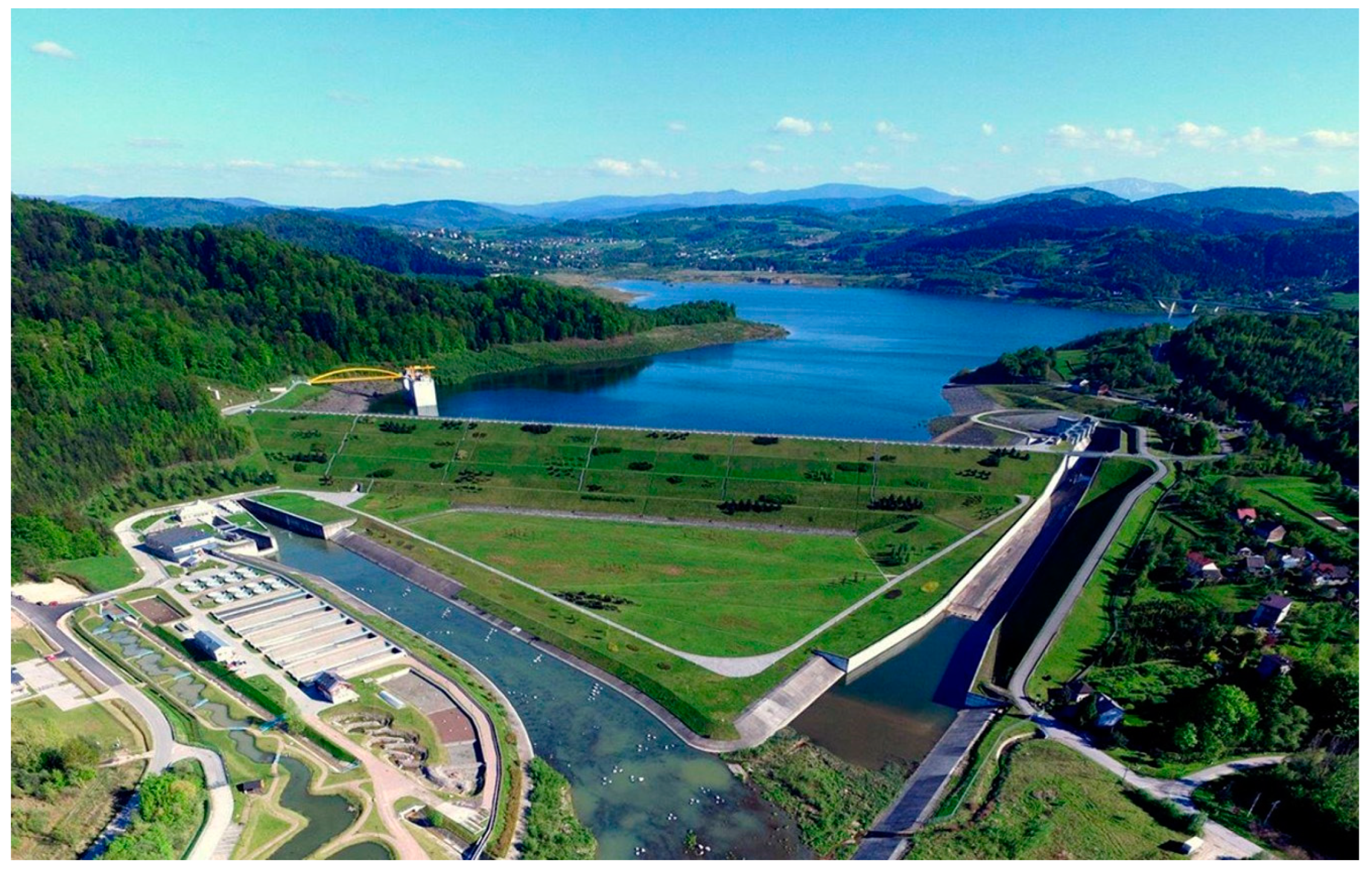
The SHP (Figure 1), which is the target of this research, is located in Lesser Poland Voivodeship, in the Municipality of Zator, at 8880 m of the Skawa River (the distance to the river mouth) on its left bank. Construction work began in 2007, while the first start-ups, and, thus, the first transfer of electricity produced from this SHP to the power gird, took place in 2012.

In the SHP building is a control system, measurement devices, and two hydro-sets (generators: Siemens, Munich, Germany, turbines: Wodel, Nowa Sól, Poland): an electric generator 550 kW with Kaplan turbine with installed discharge of water = 8 m³/s and an electric generator 210 kW with a Kaplan turbine with installed discharge of water = 5 m³/s. The SHP uses damming, which is provided by a permanent concrete weir with a flushing outlet. This weir was built to capture water for municipal purposes and to provide water for nearby fish ponds. The overflow surface has the shape of a trapezoid with a wall inclination of 1:1.5. The water that causes turbines to rotate enters through the inlet of the concrete canal, the entrance of which is secured with water intake gratings in order to prevent unwanted waste transported in the river current from entering the turbines (i.e., fragments of river vegetation, pieces of wood, anthropogenic waste) that may disturb the functioning of the SHP or cause damage to the turbine rotor. Water is processed by turbines out through the outlet part of the channel.

The forecasts were made to predict the hourly electricity production (kWh) of the selected SHP in 12 and 24 h horizons. These data for training and testing were received from the private owner of the SHP, who receives a commercial report every month via e-mail from a company intermediating in the sale of energy to the power grid. The second hourly parameter obtained from the SHP was a nominal head (as explanatory variable), understood as the difference between upper and lower water levels. Upper water level is, additionally, regulated by an inflatable rubber dam installed on the weir. For this reason, nominal head can be up to 6.37 m (5.8 m without rubber dam).

2.2. Skawa River and Data from Meteorological Stations and Water Gauge

The river the SHP uses is called Skawa. It is a right-bank tributary of the Vistula River and represents the nival–pluvial river regime. The length of Skawa is 96.4 km. The Skawa drainage basin is 1160 km². The stream bed of Skawa is entirely located in Lesser Poland Voivodeship. This river has a high flood potential, characterized by sudden but short-lasting floods. Therefore, it is described by a large amplitude of flow variability. The Skawa flows into the Vistula River near the town of Smolice, just behind the water barrage, which is a part of the Upper Vistula Waterway. Below Wadowice, Skawa meanders, flowing on the flat bottom of the valley. In the areas of Zator and Wadowice, it is accompanied by a complex of fish ponds. Due to the natural values that attract numerous species of water and marsh birds, the NATURA 2000 area Lower Skawa Valley PLB120005 was established [25,26].

The Skawa uses groundwater and surface runoff that come from precipitation and snowmelt. The anthropogenic source of water for the Skawa is the Świnna Poręba reservoir. The data related to the weather conditions affecting the flow of the Skawa were obtained from the Institute of Meteorology and Water Management—National Research Institute. The hourly data were received from the beginning of September 2018 to the end of June 2022 from three meteorological stations and one water gauge station, which are located below the reservoir and above the SHP (Figure 2).

The following explanatory data were obtained: Inwałd Meteorological Station—precipitation (mm), air temperature (°C), and wind speed (m/s); Kalwaria Zebrzydowska Meteorological Station—precipitation (mm); Wadowice Meteorological Station—precipitation (mm); Wadowice Water Gauge Station—flow (m³/s) and water level (cm) of the Skawa River. The above stations and the reservoir are located 12 to 20 km from the SHP.

2.3. The Świnna Poręba Reservoir

The SHP under consideration also uses flow provided by the water discharged from the water reservoir in Świnna Poręba (located in three municipalities: Mucharz, Stryszów, and Zembrzyce, Lesser Poland Voivodeship, Poland). The water retained by this reservoir is called Mucharskie Lake (Figure 3). The first construction work began in 1986 and its completion was announced in 2017. The maximum filling of the reservoir is 161 million m³, and its area at maximum is 1035 ha. The dam is 604 m long and 54 m high [27]. This reservoir serves the following useful functions [28]:

• ensuring flood safety below the dam, in particular, around Wadowice and Kraków, by reducing the amount of flood water that the Skawa River carries to the Vistula River,
• water retention to mitigate the effects of drought by increasing the flow of the Skawa River, especially in the summer months, which are characterized by low precipitation and high air temperature,
• drinking water reservoir for the local towns of the province: Lesser Poland and Silesia,
• energy use of water for electricity production released by the hydropower plant (4.4 MW),
• recreational use and increase in tourist activity in the region (walking, sailing, fishing, etc.).

The SHP located below the reservoir benefits the most in the summer due to the equalization of river flow through the discharge of water accumulated in the reservoir during more frequent and intense rainfall. The negative effects of drought, which causes low flows, are eliminated. This reservoir guarantees a water outflow giving the Skawa River at least 5 m³/s.

The data for creating forecast models related to the impact of the Świnna Poręba Reservoir on the functioning of the analyzed SHP were obtained from the National Water Management Company—Polish Waters in Kraków. The following data were received from September 2018 to June 2022: water outflow from the reservoir (m³/s), average daily water inflow to the reservoir (m³/s), filling the reservoir with water (million m³), free reservoir reserve (million m³).

2.4. Data Preparation

When analyzing the data, there may be variables that are significantly different from the others. They are called outliers. Such data can disrupt the model creation process and reduce the quality of the forecast. Outliers may have different sources, e.g., an error in the measurement system, errors made by the people who take measurements, improperly selected methodology, or rare and/or extreme events. The detected outliers were eliminated from the dataset [30]. The most common anomaly in forecasting was time without electricity production, which was removed first. The longest continuous period of downtime of the SHP was caused by a failure of one of the turbines: due to an incorrect fixing after 8 years from the start of the SHP, the rotor blades were damaged, the repair of which took a long time (the longest break for renovation lasted from 26 July 2021 to 14 August 2021). Historical data indicated the possibility of electricity production, but it was not possible to measure the electricity produced due to the power plant being shut down for repairs. Short-term readings without the production of electricity were caused by planned stops of devices in order to check the technical condition of individual components of the installation (mainly checking the tension of the transmission belt), automatic shutdown of the SHP during a reduced and disturbed flow of the river water stream, which was caused by the accumulation of material transported by the river onto the grates, and, consequently, the clogging of the inlet chamber (the automatic grate cleaner is not included). Only when the employees removed debris on the grate did the SHP start working again. The shutdown of the unit was also caused by planned inspections and renovations of the power grid or by a failure of the power grid (e.g., errors made by employees, transmission lines torn down by broken trees during a storm, the icing of these lines in autumn and winter).

The Interquartile Range (IQR) was chosen as the first method to identify outliers after eliminating hours with no electricity production. For one particular attribute, the first quartile (Q₁) and the third quartile (Q₃) are calculated, and then the IQR [31].

IQR = Q₃ − Q₁

(1)

After determining the IQR for each variable, the values falling outside the range created by the formula were considered outliers.

(Q₁ − 3 ∙ RQ, Q₃ + 3 ∙ RQ)

(2)

The collected data related to meteorological and hydrological conditions were not always complete. There were shortages lasting several hours, very rarely lasting several days. This was caused by failures of the measuring instruments, as well the software responsible for reading and writing data. If data were missing, such observations were not removed, but an imputation (supplementing) of the missing values was used. The k-Nearest Neighbors (k-NNs) was used for this purpose. The estimator of k-NN regression function f is defined as the arithmetic mean of the explained variables y in the vicinity of the explanatory variable x. The neighborhood is determined by the value of the parameter k nearest (in the sense of the adopted metric) neighbors of the variable [32]:

$$f\left(x\right)={\displaystyle \frac{1}{k}}{\sum }_{i\in {\Theta }_k\left(x\right)}{y}_i$$

(3)

where Θ_k (x) is the set of indices of the k-NNs of the variable x.

The k-NN method is classified as a multiple imputation. Such methods involve generating from several to a dozen different sets with completed data using k-NNs. The generation of these sets of missing data reflects the uncertainly of the value that should be substituted for the missing value. Each set of completed data is then analyzed separately, resulting in k partial parameters. In the next step, the resulting parameters are calculated as average values. Murti et al. (2019) [33] found that the results of finding missing data with the k-NN method can reach the accuracy of complete data in each case with a low accuracy difference. The robust imputation of missing value strategies like k-NNs promise to improve forecasting accuracy and reliability, particularly in domains where accurate predictions are crucial for decision making [34].

2.5. Selection of Parameters Included in the Forecast Models

The selection of parameters that have an impact on electricity production in the SHP was carried out using two methods. The Boruta Package was used first (a library in R and Python is available). It is an algorithm that adds additional weakly relevant features called “shadows” to an existing dataset. “Shadows” are used as a reference to evaluate the relevance of the original attributes of the data to be analyzed. The attribute-importance-based comparison measures the usefulness of each variable for which estimates are made by machine learning systems during training, which uses Random Forests (RFs). This allows for the recognition of complex dependences between variables that are stochastically selected for the model. The importance of less important variables is well estimated. The advantages of this method are resistance to overfitting and no requirement to optimize hyperparameters. Additionally, the Boruta Package performs the selection iteratively: variables that are considered irrelevant are gradually removed from the dataset, allowing for a more accurate assessment of the importance of remaining attributes, which translates into the increased stability and accuracy of the entire algorithm [35].

The second method used to select variables was the Variance Inflation Factor (VIF), which is computed for the i-th feature using the following formula [36]:

$${\mathrm{VIF}}_{\mathrm{i}}={\displaystyle \frac{1}{1-R_i^2}}$$

(4)

where: $R_i^2$—coefficient of determination for the multiple regression model between the i-th explanatory variable and all other explanatory variables.

It measures which part of the estimator’s variance is caused by the fact that the i-th variable is not orthogonal to the other explanatory variables in the regression model. The VIF is calculated for each explanatory variable (predictor) separately, making it possible to determinate which variables introduce multicollinearity into the model. When the VIF > 10, multicollinearity is disturbing, and the variable responsible for it (redundant) is removed from the model.

2.6. Artificial Neural Networks

Artificial Neural Networks (ANNs) were developed on the basis of the structure and operation of biological systems. They owe their name to the pattern in which the connections between individual components resemble the structure of connections between nerve cells: neurons. A single artificial neuron as a computational unit calculates an output value based on the weighted sum of the input data. Parameters entered into the network from inputs X = x₁, x₂, … x_n that simultaneously affect an artificial neuron, the value of which depends on the weighted sum of inputs and the current weights W = w₁, w₂, … w_n [37,38].

2.6.1. Multi-Layer Perceptron

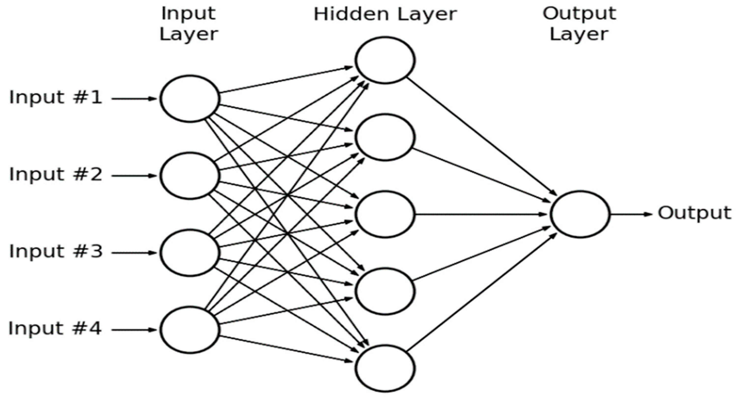
One type of neural network consisting of many artificial neurons is the Multi-Layer Perceptron (MLP). It is a one-way ANN, where neurons are connected between layers according to the “peer-to-each” principle, and there are no connections in one layer. There are three basic types of layers: an input layer, which is responsible for transmitting signals collected from the environment to the inputs of neurons in the next hidden layer, where data are processed and an output signal is generated, which is transferred to the input of the next hidden layer or to the last output layer (Figure 4). In the output layer, a value of the entire network is, finally, calculated [39]:

$$\mathrm{x}={\sum }_{i=0}^p{w}_{j,i}\cdot u_i$$

(5)

where:

• p—number of inputs in the j-th neuron,
• w_j,i—value of the weight representing the connection between j-th neuron and its i-th input,
• u_i—value occurring at the i-th input of the neuron.

In this study, the activation functions in the hidden and output layers were linear, sigmoid, hyperbolic tangent (tanh), and exponential. The Broyden–Fletcher–Goldfarb–Shanno (BFGS) algorithm was chosen to train the MLP. The quality of the training and testing processes was determined based on correlation coefficient. Forecast models of MLP were created based on the error function, which was the Sum of Squares (SOSs) of the differences between the set values and those obtained at the outputs of each output neuron. The Sum Square Error (SSE) indicator with the following formula was obtained [41]:

$$SSE={\Sigma }_{p=1}^R{\Sigma }_{k=1}^M{(d_{pk}-y_{pk})}^2$$

(6)

where:

• d_kp—model answer that should appear when presenting the training case number p at the output of the network number k,
• y_pk—the actual value that appeared on the output.

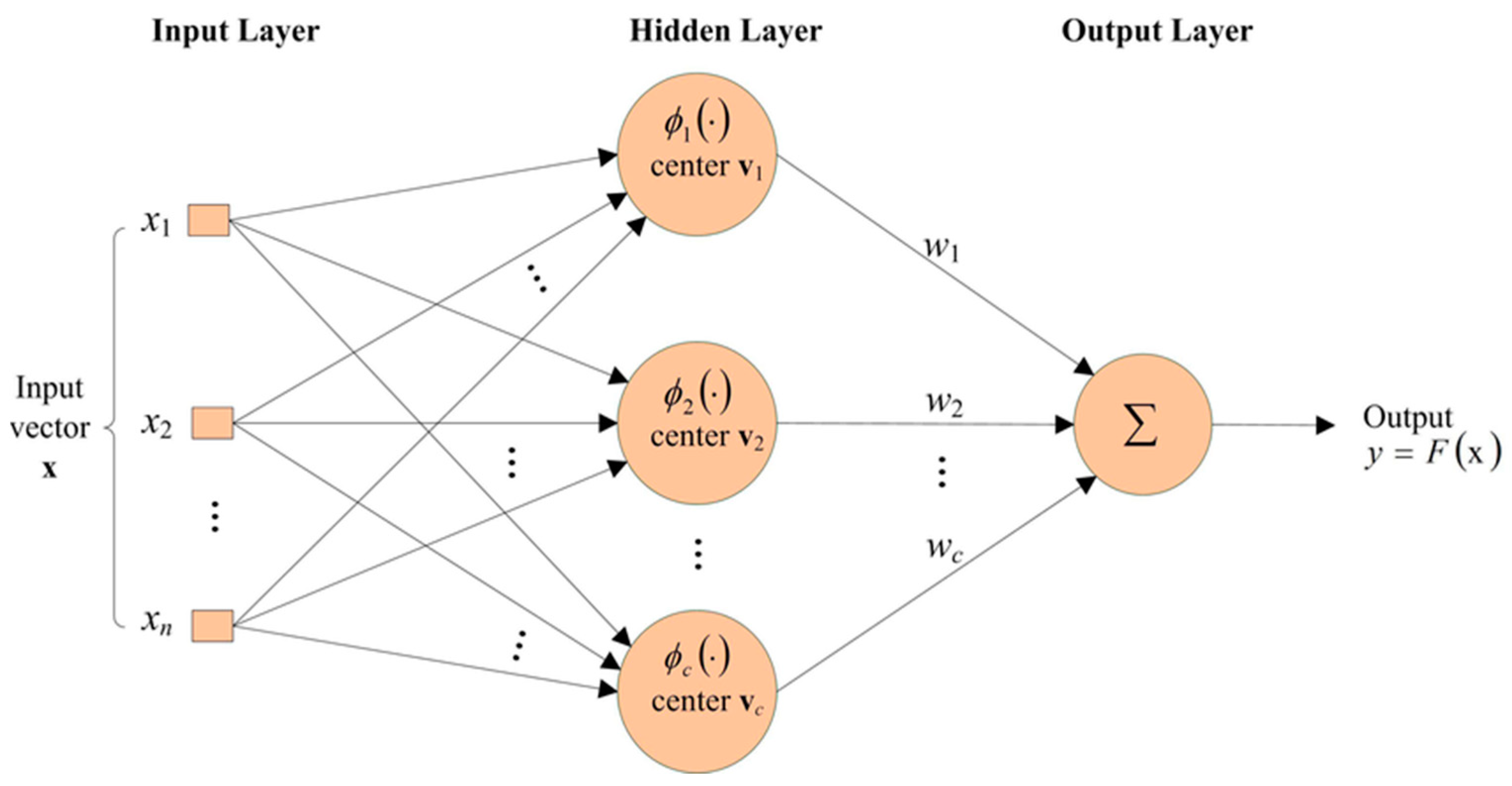
2.6.2. Radial Basis Function Networks

The second ANN used in this case was the Radial Basis Function network (RBF). It consists of three layers (Figure 5). The first is an input layer, in which the input vector of neurons forming the next layer is formed. The next one is a hidden layer in which neurons perform a radial basis function as an activation function that changes radially around the selected center of neuron c. Neurons aggregate the data entered at the input, determining the distance between input vector x and center of neuron c. The Euclidean distance was used for these calculations. The last output layer consists of the linear neurons and network response that are obtained from this layer [42].

The Gaussian function was used as an activation function in a hidden layer and the linear function in an output layer. The output values of the RBF network are estimated as the summation of the output signals of subsequent radial neurons multiplied by the appropriate weights [44]:

$${\mathrm{y}}_{\mathrm{k}}={\sum }_{j=1}^n{w}_{jk}G+b_k$$

(7)

where:

• y_k—output of the k-th output neuron,
• w_jk—weight parameter between the output of the j-th neuron in the hidden layer and the k-th neuron in the output layer,
• G—base function (activation),
• b_k—bias (additional neuron input, the weight of which is subject to the training process) of the k-th neuron in the output layer.

In the case of RBF for making forecast models, the Radial Basis Functions under Tension (RBFT) algorithm was used for training, enabling multidimensional interpolation. The centers of radial functions are determined in the hidden layer, and then the weights of neurons in the output layer are determined [45]. For RBF, the SOS function was selected as the error function, similarly to the MLP.

2.7. Decision Tree Models

A decision tree is a functional structure with attributes as input and decisions as output. Each tree is an abstract model allowing for the definition of data rules. In this approach, a single tree consists of nodes and connections between its nodes. The first node can be further referred to as the root of the tree, the intermediate nodes as its branches, and the terminal nodes as its leaves. The connections between trees are rules for dividing data into subsets according to a simple condition, and one tree provides a recipe for calculations for classification issues or predicting regression problems. The many types of decision tree method may differ in their advantages and disadvantages, but, in general, they can be described as useful under uncertain data and risk conditions [46].

2.7.1. Random Forests

The Random Forests (RFs) create a series of shallow decision trees (Figure 6). Together, these trees form a forest, and the prediction result is the result of the weighted sum of predictions from every tree. Each new tree is based on a random sample of the data obtained by random sampling with replacement (bootstrap method) and a few simple divisions after the variable values, which will result in the simple clustering of the data. For regression, the split into subsequent subsets occurs as a result of passing through all input variables and selecting such a variable and such a division that will minimize the variance for the samples in newly created nodes. The potential division is based on values, which take successive samples of a real variable, more precisely based on the average of two adjacent and consecutive samples after sorting them in ascending order. For each division, the average actual value of samples in the group is calculated, followed by calculating the square of the deviation from the group mean for each sample in the group and the sum of these squares. The smaller this sum, the greater the goodness of the given person division. Finally, a division is selected that will minimize the sum of squared errors, i.e., the total variance [47].

Formally, an RF is a predictor consisting of a collection of randomized base regression trees {r_n (X, Θ_m, D_n), m ≥ 1}, where Θ₁, Θ₂, … are independent and identically distributed outputs of a randomizing variable Θ. These random trees are combined to form the aggregated regression estimate [49]:

r¯_n(X, D_n) = E_Θ [r_n(X, Θ, D_n)]

(8)

where:

• E_Θ—denotes expectation with respect to the random parameter, conditionally, on X and the data set D_n.

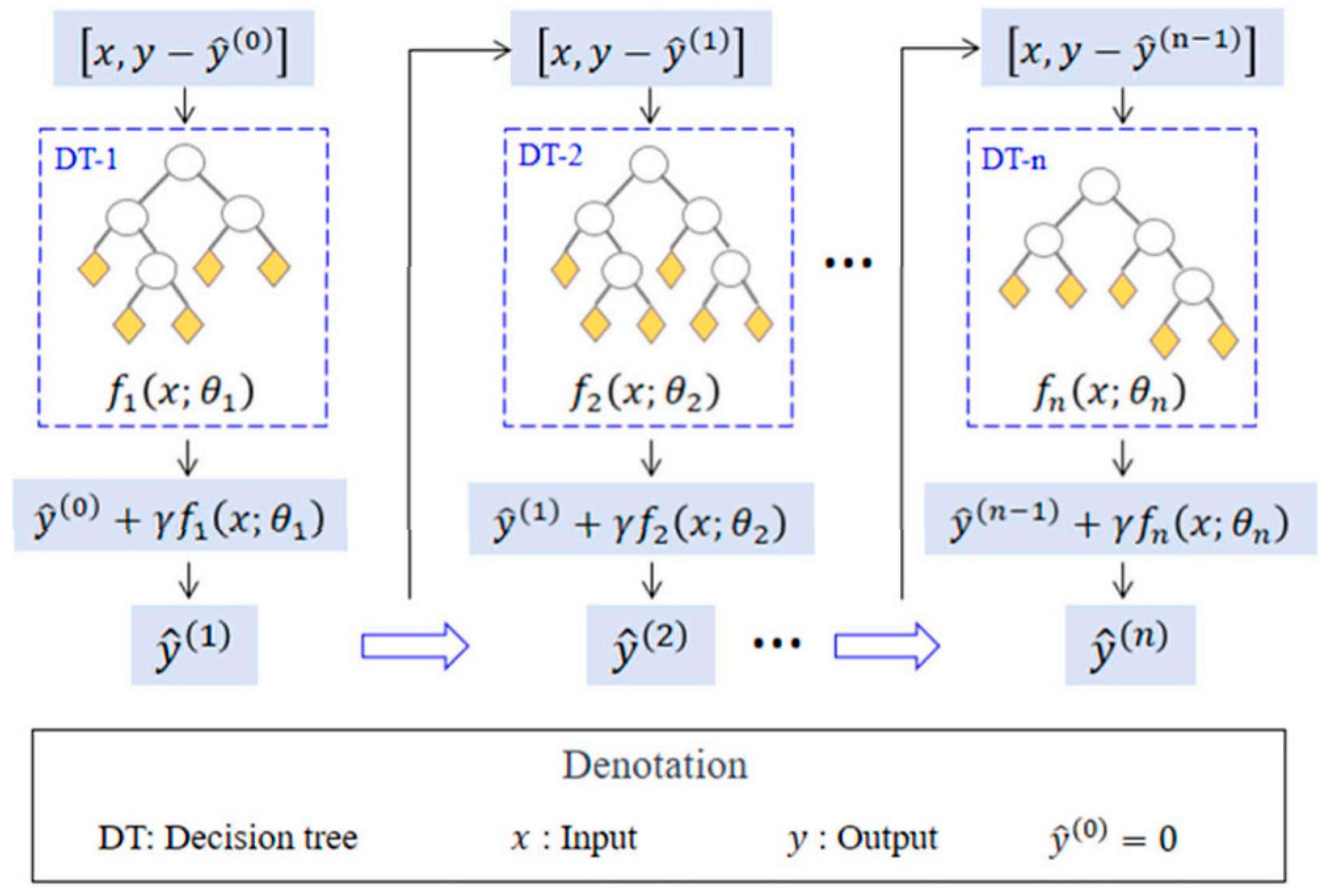
2.7.2. Gradient-Boosted Decision Trees

The Gradient-Boosted Decision Trees (GBDTs) form a weighted bundle of regression trees (Figure 7). This approach combines classification with regression. Subsequent trees are not created as predictors independent of each other, unlike for RFs. The next trees are more and more improved compared to the previous ones, and the overall forecast result is returned as the result of the sum of forecasts from individual trees. At the beginning, a hierarchy is created in data classification by dividing it into subsets. There is a data division for each variable and the division that will be allowed to achieve the highest yield is chosen, i.e., overall, it will contribute the most to reducing the error. New trees are determined iteratively using gradient and Hessian loss functions applied to the results of the trees from the previous iteration [50].

A GBDT uses weak learners to reduce the bias as well as the variance, to some degree, by reducing error. This model is a collection of linearly added weak learners:

$$\mathrm{F}(\mathrm{x},\mathsf{\beta },\mathsf{\alpha })={\sum }_{i=1}^n{\beta }_{i}h\left(x,{\alpha }_i\right)$$

(9)

where:

• h—weak learners,
• β_i—weights of each weak learner.

The GBDT sequentially grows the trees and re-evaluates the weights of each learner toward the final forecast [52].

2.8. Evaluation of Forecasts

Forecast accuracy measures are used to verify and compare different methods for creating forecast models, or the accuracy of one of the methods used in different time periods. They enable quick comparisons of models created by different authors for similar objects. These measures determine the deviations of the forecast variable from the forecasts created. They provide information as to whether the model meets certain conditions and whether it can be used. The following metrics were used to evaluate the created forecast models:

$${\mathrm{R}}^2=1-{\displaystyle \frac{{\sum }_{t=1}^n{\left(y_t-y_t^{*}\right)}^2}{{\sum }_{t=1}^n{\left(y_t-\overline{y}\right)}^2}}$$

(10)

$$\mathrm{MAE}={\displaystyle \frac{1}{n}}{\sum }_{t=1}^n\left|y_t-y_t^{*}\right|$$

(11)

$$\mathrm{MAPE}={\displaystyle \frac{1}{n}}\left({\sum }_{t=1}^n{\displaystyle \frac{\left|y_t-y_t^{*}\right|}{y_t}}\right)\cdot 100\%$$

(12)

where:

• R²—coefficient of determination,
• MAE—Mean Absolute Error,
• MAPE—Mean Absolute Percentage Error,
• y_t—value of the explained variable in period t,
• y_t^*—forecast of the explained variable in period t,
• ȳ—arithmetic mean of the explained variable,
• n—number of time units in the period.

R² describes the unpredictability evaluation with a quantitative value (from 0 to 1). If it is near 1, it tends to show that forecasted values were matched to real variables. The MAE provides information on how much, on average, during the prediction period, the forecast variable will deviate (in absolute value) from the forecast. The MAPE is an average measure and is expressed as a percentage. It is interpreted in the following way for the forecast of generating units: by what percentage, on average, does the amount of forecasted electricity production differ from the amount of energy generated in a given unit of time [53]? The dataset for the analysis has been set in the proportion of 70% for training set and 30% for testing set. In the next step, these datasets were shifted with these proportions for the validation of models in accordance with the rule of the cross-validation of time series.

3. Results

3.1. Entry Information

The hourly values of electricity production from the SHP (kWh) were forecasted. The total number of measurements was 33 576 h for each parameter. Reduction after cleansing was 33,576 − 1482 = 32,094 h for each parameter (4.41% of dataset). After data cleaning (with IQR and k-NNs), the next step was to analyze the significance of parameters with Boruta. This method classifies the predictors into three groups: important, tentative (less significant than important, the choice is left to the researcher), and unimportant. Nine parameters were chosen for checking by VIF:

• flow rate of the Skawa River from Wadowice Water Gauge Station (important),
• water level of the Skawa River from Wadowice Water Gauge Station (important),
• precipitation from Wadowice Meteorological Station (tentative),
• air temperature from Inwałd Meteorological Station (tentative),
• water outflow from Świnna Poręba Reservoir (important),
• water inflow to the Świnna Poręba Reservoir (important),
• filling in Świnna Poręba Reservoir (important),
• free reserve in Świnna Poręba Reservoir (important),
• hydraulic head near the SHP (tentative).

Three parameters were rejected:

• precipitation from Inwałd Meteorological Station (unimportant),
• precipitation from Kalwaria Zebrzydowska Meteorological Station (unimportant),
• wind speed from Inwałd Meteorological Station (unimportant).

In the next step, the mutual dependencies between the independent variables were checked (

Table 1. The VIF values between all independent variables.

Predictors	Air Temperature	Water Level	Flow Rate	Precipitation	Outflow from the Reservoir	Inflow to the Reservoir	Filling in the Reservoir	Reserve in the Reservoir	Hydraulic Head of SHP
air temperature	x	1	1	1	1	1.01	1.05	1.14	1
water level	1	x	5.11	1	5.64	1.2	1.18	1.22	1
flow rate	1	5.11	x	1	6.36	1.18	1.11	1.07	1
precipitation Wadowice	1	1	1	x	1	1	1	1	1
outflow from the reservoir	1	5.64	6.36	1	x	1.12	1.1	1.25	1
inflow to the reservoir	1.01	1.2	1.18	1	1.12	x	1.03	1.16	1
filling the reservoir	1.05	1.18	1.11	1	1.1	1.03	x	6.69	1
reserve in the reservoir	1.14	1.22	1.07	1	1.25	1.16	6.69	x	1
hydraulic head of SHP	1	1	1	1	1	1	1	1	x

). The VIF value was not greater than 10 in any case.

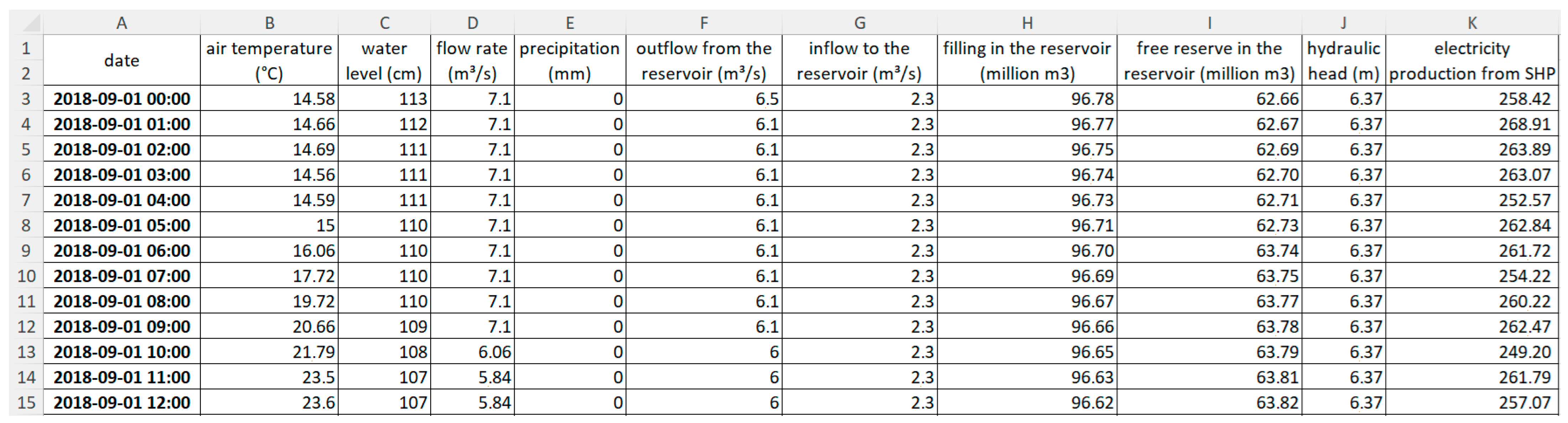
Air temperature, water level, flow rate, precipitation (from Wadowice), outflow from the reservoir, inflow to the reservoir, filling the reservoir, reserve in the reservoir, and hydraulic head were included in creating forecast models in all four methods (MLP, RBF, RF, GBDT). Figure 8 shows sample lines in the data file.

Table 2. Statistics of parameters included in the forecast models before data cleansing.

Parameters/Statistics	Min.	Max.	Arithmetic Mean	Standard Deviation	First Quartile	Median	Third Quartile
air temperature [°C]	−14.97	34.87	9.32	8.34	2.55	8.94	15.71
water level [cm]	93	276	121.43	21.1	108	111	131
flow rate [m3/s]	3.7	149	11.71	9.56	6	6.82	13.8
precipitation Wadowice [mm]	0	26	0.08	0.55	0	0	0
outflow from reservoir [m3/s]	4.2	130	11.25	11.38	5.4	6	14
inflow to the reservoir [m3/s]	0.59	251.43	11.9	19.59	3.52	6.24	12.92
filling the reservoir [million m3]	16.94	131,2	90.23	20.97	79.9	98.93	107.94
reserve in reservoir [million m3]	29.65	193.51	70.61	24.21	52.9	61.91	82.2
hydraulic head of SHP [m]	5.8	6.37	6.04	0.27	5.8	6.37	6.37

presents the basic statistics of the studied parameters before data cleansing, and

Table 3. Statistics of parameters included in the forecast models after data cleansing.

Parameters/Statistics	Min.	Max.	Arithmetic Mean	Standard Deviation	First Quartile	Median	Third Quartile
air temperature [°C]	−14.97	34.87	9.22	8.33	2.63	8.77	15.53
water level [cm]	93	176	117.43	15.13	107	109	130
flow rate [m3/s]	3.7	37.2	9.56	4.97	5.7	6.5	13.3
precipitation Wadowice [mm]	0	23	0.07	0.44	0	0	0
outflow from reservoir [m3/s]	4.2	39.8	9.38	6.64	5.4	5.6	12
inflow to reservoir [m3/s]	0.59	159.56	8.83	10.21	2.95	5.4	11.34
filling the reservoir [million m3]	16.94	119.14	80.46	26.73	51.69	91.1	105.03
reserve in the reservoir [million m3]	41.7	193.51	80.43	30.86	55.81	69.75	109.26
hydraulic head of SHP [m]	5.8	6.37	6.16	0.27	5.8	6.37	6.37

after data cleansing.

3.2. Multi-Layer Perceptron Model Results

For the time series analysis, the regression and automatic network search of StatSoft STATISTICA 13.1 were used to create the forecast using MLP. The process of searching for the best MLP ANNs started with a default of 20 networks, then 40, 60, and 80 networks were checked, ending with 100 networks because, when the number of networks exceeds 100, no increase in the quality of these networks was observed. Three highest quality ones were retained. The lagged value was set to 12. The beginning of process involved selecting data (70%) from the period from 1 September 2018 to 31 March 2021 as the training set. Data (15%) from the period from 1 April 2021 to 15 December 2021 were selected as the testing subset. For validation, data (15%) from 16 December 2021 to 30 June 2022 were selected. The results of training the MLP are presented in

Table 4. Statistics of creating MLP models for a forecast with a 12 h horizon.

ID of Network	1	2	3
name of network	MLP 132-14-1	MLP 132-12-1	MLP 132-14-1
quality (training)	0.977	0.977	0.978
quality (testing)	0.972	0.971	0.972
quality (validation)	0.972	0.971	0.971
training algorithm	BFGS	BFGS	BFGS
error function	SOS	SOS	SOS
activation (hidden layer)	exponential	hyperbolic tangent	sigmoid
activation (output layer)	sigmoid	sigmoid	hyperbolic tangent

and

Table 5. Statistics of creating MLP models for a forecast with a 24 h horizon.

ID of Network	1	2	3
name of network	MLP 132-14-1	MLP 132-12-1	MLP 132-14-1
quality (training)	0.964	0.960	0.962
quality (testing)	0.954	0.955	0.957
quality (validation)	0.952	0.951	0.952
training algorithm	BFGS	BFGS	BFGS
error function	SOS	SOS	SOS
activation (hidden layer)	sigmoid	sigmoid	sigmoid
activation (output layer)	linear	exponential	linear

.

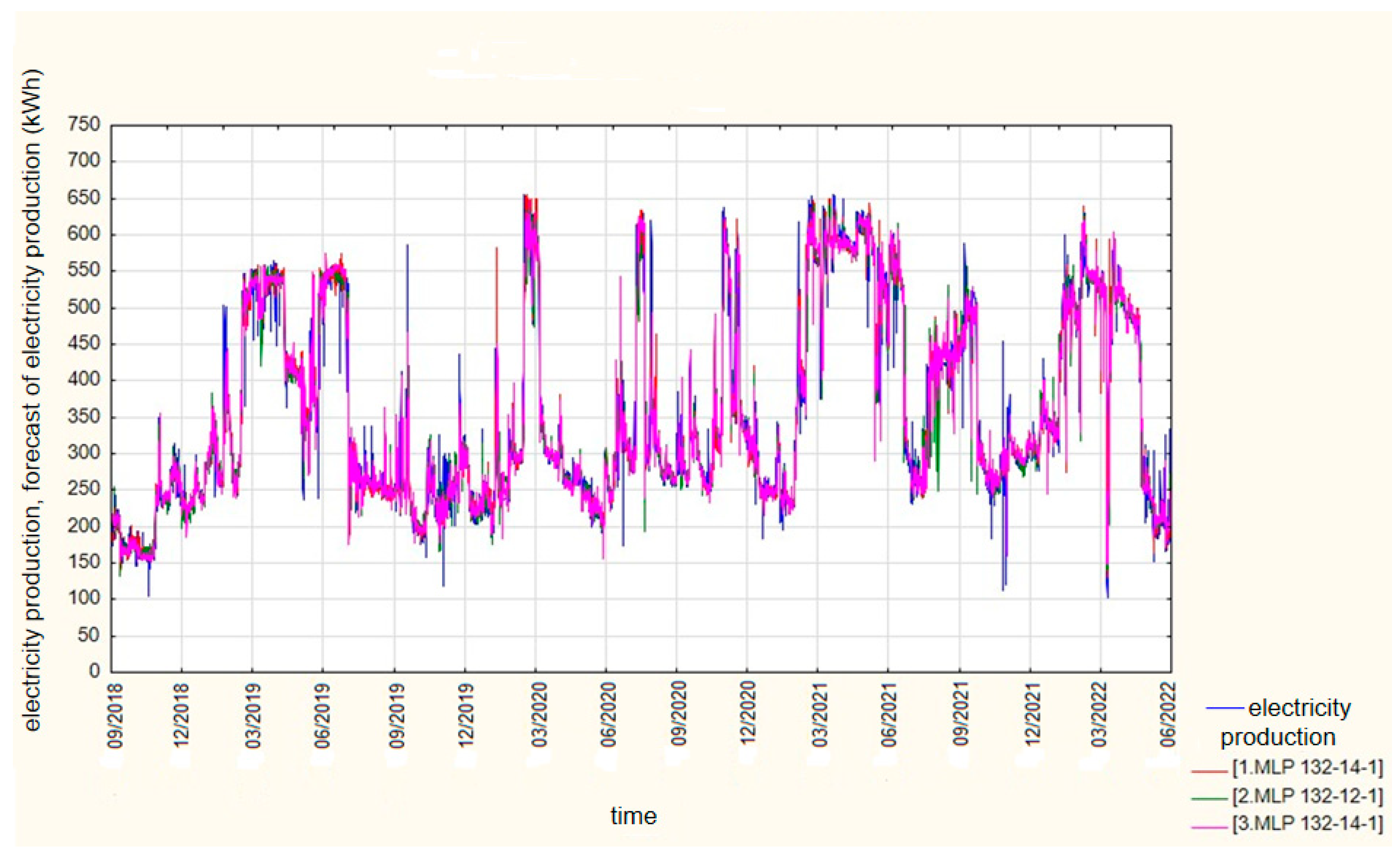
Due to the satisfactory quality of training, testing, and validation, 12 h horizon (Figure 9) predictions were made. An example MLP 132-14-1 means that there are 132 neurons in the input layer, 14 neurons in the hidden layer, and 1 neuron in the output layer.

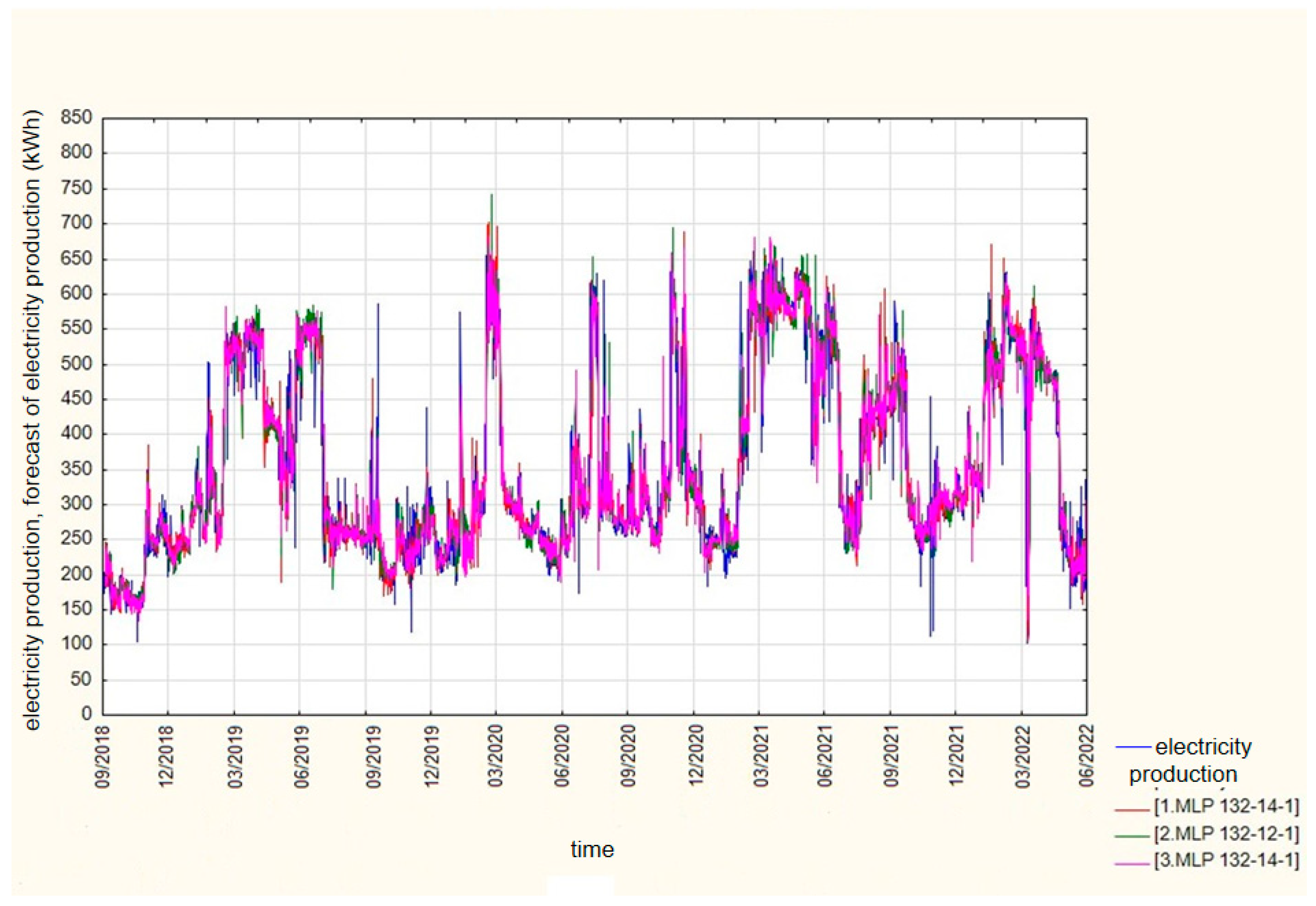
Due to the satisfactory quality of training, testing, and validation, 24 h horizon forecasts were made (Figure 10).

3.3. Radial Basis Function Network Model Results

For the time series analysis, the regression and automatic network search of StatSoft STATISTICA 13.1 were used to create a forecast using RBF networks. The idea and number of networks analyzed were the same as for the MLP and three highest quality ones were also retained. The lagged value was set to 12. The start of modeling involved selecting data (70%) from the period from 1 September 2018 to 31 March 2021 as the training set. Data (15%) from the period from 1 April 2021 to 15 December 2021 were selected as the testing subset. For validation, data (15%) from 16 December 2021 to 30 June 2022 were selected. The results of training RBF networks are presented in

Table 6. Statistics of creating RBF models for a forecast with a 12 h horizon.

ID of Network	1	2	3
name of network	RBF 132-26-1	RBF 132-27-1	RBF 132-23-1
quality (training)	0.393	0.320	0.459
quality (testing)	0.398	0.320	0.461
quality (validation)	0.394	0.308	0.456
training algorithm	RBFT	RBFT	RBFT
error function	SOS	SOS	SOS
activation (hidden layer)	Gaussian	Gaussian	Gaussian
activation (output layer)	linear	linear	linear

and

Table 7. Statistics of creating RBF models for a forecast with a 24 h horizon.

ID of Network	1	2	3
name of network	RBF 132-23-1	RBF 132-25-1	RBF 132-26-1
quality (training)	0.310	0.328	0.277
quality (testing)	0.329	0.333	0.295
quality (validation)	0.304	0.313	0.270
training algorithm	RBFT	RBFT	RBFT
error function	SOS	SOS	SOS
activation (hidden layer)	Gaussian	Gaussian	Gaussian
activation (output layer)	linear	linear	linear

.

Due to the very low quality of the training, testing, and validation of RBF networks, 12 h horizon forecasts were not created. To make a satisfactory prediction, the training, testing, and validation quality values are expected to be a minimum of 0.9.

In 24 h horizon models, the quality of the training, testing, and validation of RBF networks were also very unsatisfactory. Therefore, no attempts were made to improve these models.

3.4. Random Forest Model Results

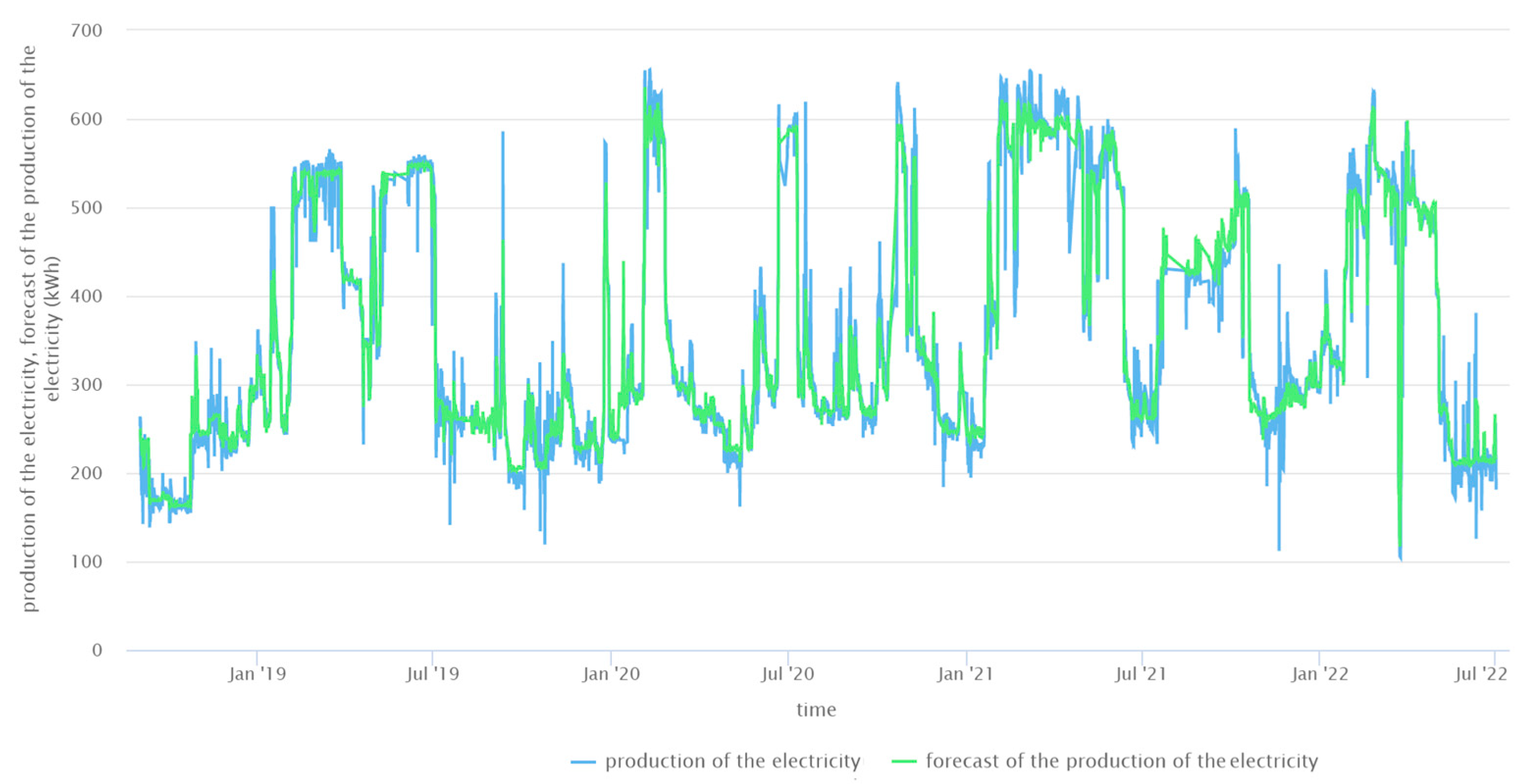
The Rapid Miner Studio Educational 10.1.003 program was used to create forecasts with the RF method. Starting with creating the models, data (70%) from the period from 1 September 2018 to 31 March 2021 were selected as the training subset. Data (30%) from the period from 1 April 2021 to 30 June 2022 were selected as the testing subset. The creation of the models started with the default 100 trees, then 200, 300, and 400, ending with 500 because, with 500 trees, there was no increase in the quality of the forecasts. This parameter specifies the number of trees generated. For each tree, a subset of examples is selected via bootstrapping. The maximal depth was 10. This parameter shows the maximal number of nodes that can be generated on each single tree. The prediction results obtained from RFs in relation to the actual SHP’s electricity production are plotted (Figure 11 and Figure 12).

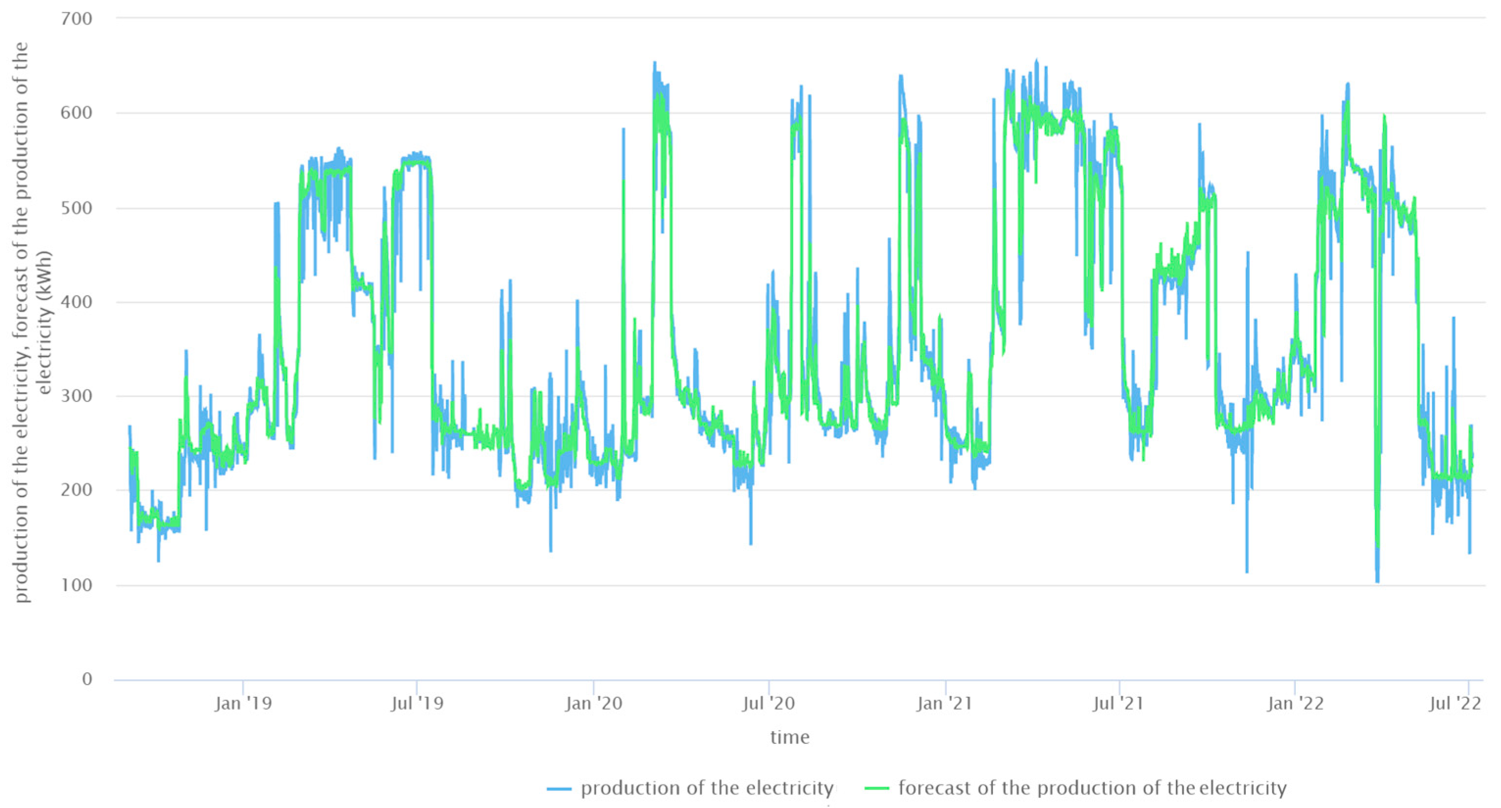
3.5. Gradient-Boosted Decision Tree Model Results

The Rapid Miner Studio Educational 10.1.003 program was used to create forecasts with the GBDT method. To start the modeling process, data (70%) from the period from 1 September 2018 to 31 March 2021 were selected as the training subset. Data (30%) from the period from 1 April 2021 to 30 June 2022 were selected as the testing subset. The number of trees was set at 500 (the number and idea of creating trees was the same as in RFs). The maximal depth was 10. The minimum row was 10. The minimum number of rows to assign to the terminal nodes was used. The number of bins was set to 20. The model build had at least the specified number of bins; these were then split at the best point. The distribution function for data training was automatically selected (from gaussian, passion, gamma, tweedie, quantile). The prediction results obtained from GBDTs in relation to the actual SHP’s electricity production were plotted (Figure 13 and Figure 14).

3.6. Evaluation of Models and Comments

Predictions were assessed with selected measures, which are summarized in two tables (

Table 8. Evaluation of the 12 h horizon forecast models.

Model	R2	MAE (kWh)	MAPE (%)
MLP 1	0.94	18.02	5.41
MLP 2	0.94	18.40	5.55
MLP 3	0.94	18.19	5.54
RF	0.98	14.91	4.66
GBDT	0.99	9.97	3.17

and

Table 9. Evaluation of the 24 h horizon forecast models.

Model	R2	MAE (kWh)	MAPE (%)
MLP 1	0.93	24.39	7.33
MLP 2	0.93	24.83	7.50
MLP 3	0.93	24.12	7.30
RF	0.98	15.84	4.96
GBDT	0.99	10.96	3.41

), separately, for a given forecast horizon.

The forecast models built for a 12 h horizon had an R² coefficient in the range of 0.94–0.99. The MAE ranged from 9.97 kWh to 18.40 kWh, while the MAPE ranged from 3.17% to 5.55%. The best result was given by a model using GBDTs. The worst model from RBF was not included into the table (because of the very low quality of training).

The forecast models built for a 24 h horizon had an R² coefficient in the range of 0.93–0.99. The MAE ranged from 10.96 kWh to 24.83 kWh, while the MAPE ranged from 3.41% to 7.50%. The best result was given by a model using GBDTs. The worst model from RBF was also not included in the table (because of the very low quality of training).

A common regularity of each model was the increase in forecast error as electricity production increased. This occurred mainly at the turn of the winter and spring months, when the river was additionally fed by snowmelt. Such increases in electricity production also occurred in autumn during heavier rainfall. The forecast curves also did not match the real electricity production during the production of energy drops caused by clogged inlet grates. This blockage lasted for several hours on some nights as the employees cleaned the grate in daylight for safety reasons. The forecasts also did not capture several increases lasting several hours caused by short intense precipitations. The lowest forecast errors occurred mainly in summer during stable flow with very small supply due to very low rainfall and high temperatures.

4. Discussion

The main idea of the selected forecasting methods (MLP, RBF, RF, and GBDT) was to find models with a simple structure and high quality of evaluation in RES prediction cases recommended by other researchers. Due to the complex structure and high computational cost, Extreme Learning Machine (ELM) and Deep Learning (DL) models were not considered. The aim of this study has been achieved. Among the selected four basic AI methods, two of them (RF and GBDT) gave predictions with an MAPE of less than 5%. Hence, there was no justification for further interference in improving individual models (e.g., using L2 regularization or dropout techniques in ANNs or changing the distribution function in GBDT). Satisfactory results were accomplished by appropriate data preparation, the selection of independent variables, and then by increasing the number of networks or trees in the models. The advantage of these models is that the satisfactory quality of the forecasts were obtained without complicated techniques or modifications that require a higher computational cost. Both decision tree methods outperform ANNs in this case. Based on forecasting experience, ANNs have specific hyperparameters (number of layers, types of layers, number of neurons per each layer, activation functions, training algorithms, etc.) and, in some cases, it is very difficult to obtain good results by ANNs with that many hyperparameters. Another advantage of decision tree models is that they have fewer hyperparameters and require less modeling experience than ANNs. Also, ANNs are prone to overfitting. RFs have beneficial options, e.g., weighting the differential layer and metrics of variable importance. RFs can also reduce mutation and increase stability in predictions. The technique of building trees on different and independent sub-models reduces the overfitting and improves the ability to generalize [54]. GBDTs can be more accurate than RFs because they are trained to correct each other’s errors; they are capable of capturing complex patterns in a dataset [55]. A single GBDT model with seasonal parameters is recommended. Small differences between the forecast value and real electricity production occurred both in the stable summer period and during the upward trend at the turn of winter and spring caused by snowmelt.

A common feature of the publications dealing with short-term forecast models of electricity production dedicated to SHPs was that the authors provided information concerning the method they used to create the models and how they assessed the obtained forecasts. They also indicated the more or less precise location of SHP units. They also provided the variables that were included in the model and which period these data came from. However, not all articles provided the basic parameter of the SHP: installed power. Globally, an SHP includes facilities with generators up to 25 MW, and models for “larger” small units will not always be applicable to power plants with a much lower installed capacity, as in the case of the SHP analyzed in this article (with an installed capacity of 0.76 MW). The number, type, and parameters of water turbines were not always provided. This would help determine possible differences when forecasting units with different types of turbines and rotor sizes. To create forecasts for a run-of-river SHP, the researchers used the RF method [56]. The authors chose air temperature, precipitation, and an installed capacity utilization factor as parameters to be entered into the models. The data came from a 3-year period and concerned the facilities from 11 European countries. For the best models, the R² was 0.9–0.95 for the for the installation from Spain, where, due to its geographical location, the flow rates are low and stable. The lowest R² in range of 0.48–0.83 concerned the units in Finland. It was found that the low R² was caused by large fluctuations in water levels due to large, frequent, and diversified precipitation, the significant supply of rivers with meltwater in spring, and non-uniform discharges of water from reservoirs. Jung et al. (2021) [11] predicted the electricity production of a specific SHP in South Korea using a classic three-layer ANN. They chose precipitation, air temperature, average wind speed, average relative humidity, and water outflows from reservoir over a 20-year period as independent variables. To evaluate these models, they used the Nash–Sutcliffe Efficiency (NSE), which, for their ANN, was 0.77. NSE is almost equivalent to R² [57]. The impact of extreme phenomena (mainly floods) was indicated as the greatest difficulty during modeling, which resulted in a reduction in the quality of forecasts. Li et al. (2014) [58] analyzed hydropower potential by comparing Autoregressive Moving Average (ARMA) models with Genetic Algorithm (GA) models combined with Support Vector Machine (SVM) in two Chinese regions: Yunlong and Maguan. They collected data of the river flow, outflow from reservoir, and precipitation for a period of 915 days. For the Yunlong region, ARMA forecasts had an MAPE ranging from 4.99% to 5.58%, while the GA-SVM models had an MAPE ranging from 5.07% to 5.19%. For the Maguan region, ARMA had an MAPE of 4.46–4.60% and GA-SVM had an MAPE of 4.32–4.40%. Slightly better results were achieved using GA-SVM. Authors recommend this method for forecasting when we have a small number of predictors at our disposal. Drakaki et al. (2022) [59] analyzed the electricity production of an SHP located in the western part of Greece using a deep one-way ANN (DNN) compared to a simple regression model. Precipitation amounts and river flow were introduced into the forecast models. R² was in favor of the DNN at 0.84, while the regression coefficient was 0.63. Yildiz and Açikgöz (2021) [16] forecasted an SHP’s electricity production using the ABC algorithm in a unit located in the eastern part of Turkey. They chose relative air humidity, precipitation, air temperature, and ground temperature as explanatory variables (historical data from 3 years). The R² results of their models were in range of 0.93–0.94, while the MAE results were in the range of 5.75–6.51 kWh.

A further direction in the development of forecast models for SHPs proposed in this article would be to extend the period of data collection for analysis. A longer period of time over which data are collected could be used to divide the models into four groups according the seasons. In the period under study (September 2018–June 2022), there was no long-lasting frost in the winter months, which would first cause ice phenomena to form on the river—drifting ice, then ice floes—which would cause an ice jam on the river. Ice piles can partially block the river, disturbing its flow and increasing underwater flow, which may contribute to flooding. When there is a high probability of ice floes forming for a long time, SHPs are preventively turned off and river flow is directed entirely through the weir because the floe, by stopping at the inlet grates, could destroy the rotor of turbines and guide vanes. In spring, the river is expected to be supplied with meltwater (in this case, there were no snowy or frosty periods for the long period). Summer is usually associated with low flows compensated by water discharges from reservoirs, and possible floods may occur due to storms and torrential rains, which were not observed very often in the period under study. In autumn, there are significant amounts of precipitation compared to spring and summer, and more material flows through the river in the form of leaves that fall from trees in autumn. Also, in autumn, there is an increased activity of beavers, who build dams and impoundments and store food. This causes an increased amount of flowing fragments of branches, logs, and river plants that stop at the inlet grates, and frequent cleaning required during this period.

The next step would be to look for additional explanatory variables that may improve the quality of the forecast. It would be necessary to take into account the losses of the water flowing into the channel with turbines caused by the clogging of the inlet grates by material transported by the river. Autumn accumulations of debris require cleaning by an employee. During the night, grates are not cleaned, so blocking the inlet, especially before dawn, significantly reduces the amount of energy produced. In order to take these losses into account, an attempt can be made to add a new independent variable to the models by installing an underwater camera which will take photos of the grates, and then, after computer image analysis, the percentage of inlet grates that are covered by debris can be calculated. It would also be useful to measure water temperature near the SHP. Based on this, the density of the water can be determined. The density of the water that sets the turbine in motion affects the variability of the mechanical energy of the water supplied to the turbine and, consequently, the variable amount of electricity produced.

Creating even better RES forecasting models is still a current topic. Li et al. (2023) [60] draw attention to the randomness of RES, which may pose some problems for the comprehensive operation of the power grid, and short-term forecasting can help to significantly reduce the uncertainly of energy balancing. Kamiński and Kolasa (2023) [61] indicate that predictive models will help guarantee sustainable and safe synergy between conventional energy and RES. Private owners of RES units are also looking for useful tools for managing installations. Sørensen et al. (2022) [62] point out that the key issue for the best forecasts is not only the appropriate selection of methods, but also knowledge of the practical aspects of the facility’s operation, which will allow for the appropriate selection of input data to the model that will adequately reflect the functioning of RES units. The structural diversity of individual SHPs located in different sections of rivers, ambiguous rules for managing retention, and the multitude of meteorological factors influencing the final electricity production of these units make it very difficult to create a universal predictive model. The aspect of RES should be constantly developed in order to encourage entrepreneurs to invest in this type of project and ensure that the energy security of individual countries is at the highest possible level, as it is one of the most important development factors.

5. Conclusions

After conducting the multi-threaded analyses, which made it possible to obtain the short-term forecasts of the electricity production of the selected run-of-river SHP, and after confronting them with the results of the literature research, the following conclusions and statements were made:

• Among the AI methods to forecast the SHP’s electricity production, the best model was obtained by GBDT. For a 12 h horizon, MAE = 9.97 kWh and MAPE = 3.17%, and for a 24 h horizon, MAE = 10.96 kWh and MAPE = 3.41%. The worst results were achieved by RBF networks, where forecasts were not created. The three best RBF networks were characterized by very low training, testing, and validation quality (values ranged from 0.27 to 0.46).
• As the forecast horizon increased from 12 h to 24 h, forecast errors also increased. The largest increase in error after comparing two selected horizons occurred in the models obtained using MLP (increasing MAPE by 1.95%), and the smallest in GBDT models (increasing MAPE by 0.24%).
• Two methods based on decision trees, RF and GBDT, confirmed the hypothesis of this study, providing forecast models of electricity production in the selected SHP with a low MAPE (<5%). The prediction created with RF for a 12 h horizon was an MAPE of 4.66%, and 4.96% for a 24 h horizon. In the case of forecast models obtained using GBDT, the MAPE for a 12 h horizon was 3.17%, and 3.41% for a 24 h horizon. The resulting high-quality predictive models will be useful both for balancing the operation of the power grid and helping the SHP’s owners manage the functioning of the unit (arranging a periodic inspection of devices and/or choosing an appropriate energy sales system).