Short-Term Photovoltaic Power Forecasting Using PV Data and Sky Images in an Auto Cross Modal Correlation Attention Multimodal Framework

Abstract

The accurate prediction of photovoltaic (PV) power generation is crucial for improving virtual power plant (VPP) efficiency and power system stability. However, short-term PV power forecasting remains highly challenging due to the significant impact of weather changes, especially the complexity of cloud motion. To this end, this paper proposes an end-to-end innovative deep learning framework for data fusion based on multimodal learning, which utilizes a new auto cross modal correlation attention (ACMCA) mechanism designed in this paper for feature extraction and fusion by combining historical PV power generation time-series data and sky image data, thereby enhancing the model’s prediction performance under complex weather conditions. In this paper, the effectiveness of the proposed model was verified through a large number of experiments, and the experimental results showed that the model’s forecast skill (FS) reached 24.2% under all weather conditions 15 min in advance, and 24.32% under cloudy conditions with the largest fluctuations. This paper also compared the model with a variety of existing unimodal and multimodal models, respectively. The experimental results showed that the model in this paper outperformed other benchmark methods in all indices under different weather conditions, demonstrating stronger adaptability and robustness.

1. Introduction

The global energy crisis and climate change have driven the focus on renewable energy, with solar power gaining attention for its potential to reduce carbon emissions [1,2,3]. Recently, photovoltaic (PV) power has seen rapid growth worldwide, gradually increasing its proportion in the energy structure. However, its intermittent and unstable nature, especially weather-induced fluctuations, poses challenges for large-scale deployment [4]. Rapid shifts in cloud cover, particularly under partly cloudy conditions, can cause the PV output to drop sharply within minutes, complicating short-term prediction [5]. Current algorithms still struggle in these conditions, often resulting in high root mean square error (RMSE) [6]. virtual power plants (VPPs) enhance grid flexibility by aggregating distributed energy resources (DERs) like PV and wind power [7]. Unlike centralized plants, VPPs can optimize market transactions and respond to demand flexibly, but they face challenges from the fluctuating nature of PVs, especially on short time scales where rapid output changes can cause mismatches, increased storage needs, and frequency issues [8]. Therefore, accurate short-term PV forecasting is essential for enhancing VPP efficiency and ensuring stable power system operation.

The forecast horizon refers to the time duration for which a forecast predicts into the future, while the forecast resolution specifies the granularity of the forecast within this horizon. PV power generation forecasts are typically categorized into four time scales based on the forecast cycle. Ultra-short-term forecasting, also referred to as solar power generation forecasting, focuses on predictions within a range of a few seconds to several minutes. It is primarily applied in real-time grid dispatch and system congestion mitigation. In contrast, short-term forecasting generally covers a forecast cycle from 10 min to one hour ahead, serving as a crucial tool for enhancing power dispatch accuracy and optimizing unit scheduling. Medium-term and long-term forecasting, with forecast horizons extending from days to weeks, are mainly used for PV power plant operation, maintenance, and management planning [9].

Current PV power prediction methods are mainly based on a single data modality, typically categorized as traditional time-series approaches and environment-aware methods using image data. Time-series prediction models analyze historical PV generation and meteorological parameters (e.g., solar radiation, temperature, humidity) with statistical models like the autoregressive integrated moving average (ARIMA) or deep learning models like long short-term memory (LSTM), bidirectional long short-term memory (Bi-LSTM), and gated recurrent unit (GRU) to capture the long-term trends and cyclic patterns [10,11]. These methods excel under stable weather but struggle with rapid changes caused by cloud movements, which can lead to sudden drops in solar radiation. This limitation makes time-series models less effective under partially or fully cloudy conditions, significantly reducing the prediction accuracy during rapid weather shifts [12,13].

In contrast, image-based prediction methods use real-time sky or satellite images to extract visual features through computer vision techniques to monitor cloud dynamics and infer their impact on solar radiation and PV power generation [14]. Total sky imagers are especially useful for ultra-short-term solar forecasting because they can effectively track cloud movement [15]. These methods excel at responding to rapid weather changes, allowing for real-time environmental sensing. However, they lack the ability to capture long-term trends and internal system behaviors due to the absence of historical PV operational data, limiting their long-term prediction capability [16]. Additionally, the high cost of imaging equipment and the computational complexity of cloud processing restricts practical applications.

Given the limitations of single-modal approaches, recent studies have focused on combining time-series and image data for more accurate PV power forecasting through multimodal fusion [17]. Advances in deep learning models like recurrent neural networks (RNNs), LSTM, GRU, and convolutional neural networks (CNNs) have facilitated this by effectively handling sequential and visual data, allowing for deep feature extraction from diverse sources and reducing the reliance on complex feature engineering. For example, integrating historical irradiance data with visual features from sky images has proven effective in learning complex relationships, even on smaller datasets [18]. Multimodal fusion enhances PV power forecasting by integrating complementary information: time-series data capture historical trends and cyclical patterns, while images provide real-time weather conditions such as the cloud cover impact on solar radiation. This approach improves the short-term prediction by enhancing the responsiveness to dynamic weather changes while accounting for historical behavior. However, challenges remain, such as the heterogeneity of data modalities, complicating feature extraction. Previous methods like Convolutional Long Short-Term Memory (ConvLSTM) have struggled to capture necessary correlations over more extended periods [19]. Additionally, efficient synergy in feature fusion is complex, with simple methods often leading to redundancy or information loss [20]. Thus, developing more intelligent fusion strategies is essential to fully leverage the complementary nature of multimodal data.

To address these challenges, this paper proposes a multimodal PV power generation prediction framework based on a cross-modal attention mechanism. The cross-modal attention mechanism dynamically identifies and prioritizes the most relevant information from each modality, enabling the model to learn complex interdependencies between modalities and improve feature representation. The framework aims to intelligently focus on the key information in different modalities that is most relevant to the prediction task and realize the deep fusion of temporal and image features. Deep fusion, in this context, refers to leveraging the cross-modal attention mechanism to deeply learn and integrate complementary features from different modalities. This allows the model to effectively capture and utilize the deeper relationships between time-series and image data, ensuring that the unique strengths of each modality are maximized for improved forecasting performance. Specifically, we designed a novel auto cross modal correlation attention (ACMCA) mechanism that can automatically capture the correlation between temporal and image data, fully integrate multimodal features, and enhance the complementarity of information between different modal data. This framework effectively utilizes the complementary benefits of multimodal data to boost the model’s prediction performance and demonstrates strong adaptability to handle complex variations across different weather conditions. Furthermore, it was designed to ensure practical applicability in real-world scenarios by adapting to diverse geographic and meteorological conditions. By integrating local meteorological data and real-time sky images, the model can address varying solar irradiance levels, cloud dynamics, and seasonal fluctuations. Its flexible structure also allows for the customization of different VPP configurations, enabling optimized forecasting under specific operational requirements. The primary contributions of this paper are as follows:

• An end-to-end multimodal prediction framework based on an attention mechanism for short-term PV power generation prediction is proposed. This framework can effectively fuse timing data and image data and substantially enhance the prediction accuracy.
• A novel auto cross modal correlation attention mechanism was designed to automatically capture the correlation between timing and image data, fully integrate multimodal features, and enhance the information complementarity between different modal data.
• The effectiveness of the proposed method was validated using real-world datasets, combining historical PV time-series data and sky images. Under consistent experimental conditions, the model outperformed other state-of-the-art methods in accuracy and efficiency across forecast horizons of 10 to 20 min.

2. Related Works

Accurate prediction of PV power generation is essential for power system operations and has emerged as a significant research area. Current approaches are divided into time-series, image-based, and multimodal learning techniques. Traditional time-series forecasting relies on historical PV data to capture cyclical and trend changes. Early statistical models, such as support vector machines, Markov chains, autoregressive models [21,22], and regression models [23,24], handle both linear and nonlinear data but adapt poorly to environmental changes, making it hard to predict PV fluctuations caused by weather effects [25]. Later, ensemble learning methods using artificial neural networks, Gaussian process regression, and random forests were employed to address the limitations inherent in standalone systems [26,27]. However, these traditional models struggle with representation learning when the data volume increases. Deep learning models like RNN were then applied to PV forecasting, but issues like gradient vanishing and explosion remained. LSTM and GRU addressed these problems with gating mechanisms, effectively capturing long-term dependencies. These have been widely applied in PV forecasting with positive results [28], but they often overlook real-time weather changes, limiting their short-term prediction accuracy.

Recently, remote sensing and imaging techniques have provided diverse data sources [29] including ground-based sky images and satellite imagery [20,30] to support various forecast horizons. Due to their ability to accurately depict cloud dynamics, sky photos have quickly gained interest in ultra-short-term solar forecasting [20]. CNN-based methods utilizing spatial features in sky images have shown strong performance in hourly solar forecasts [31]. Transfer learning offers additional benefits for prediction models by leveraging knowledge from a source domain, particularly valuable when training data are limited [32]. For instance, convolutional LSTM models have been used to extract spatial and temporal features from sky images [20], effectively learning spatio-temporal correlations and achieving minor errors over short time ranges. Despite improvements, handling multimodal data, such as integrating sky images with historical sequences, remains challenging. Using an improved U-Net model in conjunction with global and texture data [33], an infrared picture export method was presented in [34]. Predictions were then produced by combining the retrieved features with historical multi-source data. The Pred-Net backbone was enhanced to estimate multi-step-ahead surface sky images [35,36], significantly improving the model’s performance in predicting slope events [20]. A new 3D VGG-like model was created to simultaneously learn temporal and spatial information from a series of sky images, with an in-depth exploration of configurations addressing the sequence length and image resolution [37]. While these models excel at extracting features from image data, they may overlook the historical operational characteristics of PV systems.

Multimodal data fusion methods improve the prediction performance by combining data from different sources, such as historical time-series and sky images, in order to fully utilize the complementary nature of each modality [38]. The core idea of multimodal learning is to utilize the complementarity between modalities to reduce redundant information and improve the feature representation of the model [39]. In PV power forecasting, multimodal learning can simultaneously process sky images and historical sequence data to enhance the comprehensive feature representation of the model. Several studies have attempted to use multimodal fusion. Earlier approaches mainly fused multimodal features by simple feature concatenation or weighted averaging [34,37]. However, this approach fails to fully explore the deep correlations between different modalities, which may lead to information redundancy or loss of essential features. Cloud trajectories were tracked by combining a cloud-matching algorithm with a speeded-up robust feature (SURF) [40,41]. After that, a modified AM-LSTM was used to examine correlations with previous numerical data using the generated cloud motion matrix. This approach demonstrated excellent prediction accuracy, maintaining a normalized root mean square error (NRMSE) of 5.39% over a 10-min average. A CNN model using multiple input data was created, such as historical PV output, sky images, and strong regularization techniques, improving the forecast skill by 16.3% in cloudy conditions and 15.7% under all weather conditions [42]. Convolutional long short-term memory was employed for feature extraction from images, while standard LSTM was used for time-series encoding [30]. For 30-min-ahead predictions, this approach produced an NRMSE of 5.57% by combining an enhanced attention mechanism (AM) with a dynamic region of interest (ROI) to improve feature representation. Correlations between historical data and optical flow maps created from satellite photos were captured using a unique graphical learning technique [43]. This method learns both temporal and spatial correlations, enhancing the feature comprehensiveness. The work in this paper enables the efficient capture and quantification of the deep correlation between time-series data and image data to achieve an efficient fusion of multimodal features, which enhances the accuracy and robustness of PV power generation prediction compared to existing methods.

3. Data and Preprocessing

3.1. Data

Stanford University, situated at the center of the San Francisco Peninsula in California, is where the study dataset was gathered between May 2017 and May 2018. The data spanned an entire year to capture seasonal variations. Stanford University has a warm-summer Mediterranean climate, denoted on climate maps as Csb (C = temperate climate, s = dry summer, b = warm summer) by the Köppen Climate Classification System [44]. It is characterized by mild climate, dry summers, and warm temperatures. The region has long, mostly sunny summers and short, partly cloudy winters [45]. The two data types collected were sky images and PV measurements, as detailed in Section 3.1.1 and Section 3.1.2.

3.1.1. Sky Image

A 6-megapixel, 360-degree fisheye camera (type Hikvision DS-2CD6362F-IV, manufactured by Hikvision, Hangzhou, China) was installed atop Stanford University’s Green Earth Sciences building to record the sky video. Throughout the recording, the camera’s parameters (aperture, white balance, and dynamic range) remained consistent. Example sky photos in various weather circumstances are shown and illustrated in Figure 1. The video was compressed at a bit rate of 2 Mbps and recorded at a resolution of 2048 × 2048 pixels with a frame rate of 20 frames per second (fps). Pictures were downsampled to 64 × 64 pixels and extracted in the .jpg format at predetermined intervals. The resolution of 64 × 64 pixels was chosen as it balances computational efficiency with forecast accuracy. Previous studies have demonstrated that this resolution is sufficient for PV output forecasting while retaining reasonable training time, making it an optimal choice for this work [46]. Images were taken between 6:00 a.m. and 8:00 p.m. local time and did not contain images without corresponding PV output data.

3.1.2. PV Power

The PV power statistics were obtained from a solar array situated atop the Jen-Hsun Huang Engineering Center at Stanford University, located at a proximity of 125 m from the camera, a distance that is insignificant in relation to the magnitude of the clouds. The polycrystalline panels possessed a capacity of 30.1 kW-DC, with a tilt angle of 22.5° and an azimuth angle of 195°. The PV output was quantified using a “PowerLogic ION7330” power meter with an accuracy of ±0.5%, recording data to the “eDNA” historian at intervals ranging from one to ten seconds. The elevated precision and logging frequency rendered power measurement uncertainty insignificant for the examination of forecast errors. The recorded data were interpolated into a second-by-second series and averaged to minute-level data for utilization as forecast targets and input features.

3.2. Data Processing

The preprocessing of the entire dataset consisted of processing the raw PV historical numerical data as well as processing the images.

For PV data preprocessing to obtain the prediction target of minute-average output, we followed three main steps. First, interpolation: Irregularly recorded PV values were interpolated using linear interpolation to create a uniform 1 Hz time series spanning from 1 May 2017 to 1 May 2018. The interpolation process calculated the elapsed time from the initial timestamp to align all data points temporally. Subsequently, these interpolated values were aggregated into 10-s intervals by retaining the first value in each window, ensuring temporal consistency while preserving key trends in the PV output data. Second, rolling average: To align with typical forecasting targets, we converted the series to minute averages using a rolling window of 60 data points, covering 30 s before and after each minute mark. This choice ensured that the series reflected the smoothed short-term variations while maintaining the temporal resolution necessary for accurate forecasting. The selected size aligned with established practices in PV power forecasting and balances smoothing effectiveness with computational efficiency. Finally, filtering: We excluded PV outputs below zero (nighttime standby consumption) and any records with gaps exceeding one hour, typically due to maintenance.

Specifically, for any given point $m$ in the synchronized time-series $T_m$ and $P_m$, which represent the rolling averages after the second step, the point will be removed if it meets any of the following criteria.

$$T_{raw}\left(T_m,Left\right)+1h<T_{raw}\left(T_m,Right\right)$$

(1)

$$P_m<0$$

(2)

where $P_m$ denotes the PV output after rolling averaging at time $T_m$, with $m$ serving as the ordinal index for both $P_m$ and $T_m$. $T_{raw}\left(T_m,Left\right)$ represents the nearest point to $T_m$ on the left in the original recorded time-series $T_{raw}$, while $T_{raw}\left(T_m,Right\right)$ indicates the nearest point on the right.

For the image data, the original high-resolution image frames (2048 × 2048) were acquired by taking a snapshot of the original skyshot video clip at the specified frequency. The dataset utilized in this study was sampled at a frequency of 2 min, which has been validated as optimal for capturing cloud dynamics while balancing information richness and computational efficiency [42]. Increasing the sampling frequency beyond 2 min shows minimal performance gains but significantly increases the training time. Thus, 2-min sampling effectively captures cloud motion patterns relevant to PV predictions without added computational overhead. The high-resolution image frames were subsequently downsampled to a lower resolution (64 × 64) to optimize training efficiency. Subsequently, erroneous duplicate images resulting from occasional OpenCV video decoder anomalies were filtered out. Finally, the processed images were aligned temporally with the concurrently processed PV generation data.

3.3. Data Partition and Cross Validation

The processed dataset was divided into a training set (including validation) and a test set. The test set consisted of 10 manually selected sunny days and 10 cloudy days from 1 May 2017 to 1 May 2019, while the rest formed the training set. These days were chosen to ensure a balanced evaluation across varying weather conditions. Sunny days assess the model’s performance under stable conditions, while cloudy days test its ability to handle complex, dynamic scenarios caused by cloud movements. The selection spanned different months to capture seasonal variations, providing a comprehensive assessment of the model’s robustness and generalizability. The model’s training and test samples were 54,738 and 6014, respectively, maintaining a 90%:10% ratio. Figure 2 shows the PV output curves for the 20 test days, where sunny days exhibited smooth sinusoidal shapes, and cloudy days featured irregular fluctuations. Some cloudy days had sharp short-term fluctuations (Cloudy_9), while others showed minor random jitters (Cloudy_1) or consistently low output throughout the day (Cloudy_7).

Table 1. Information statistics for the 10 sunny days and 10 cloudy days used in the test set.

Date	Index	Mean (kW)	Max (kW)	Std (kW)
20 May 2017	Sunny_1	14.93	24.56	8.34
4 June 2017	Sunny_2	15.25	25.41	8.66
6 July 2017	Sunny_3	14.16	23.93	8.16
19 August 2017	Sunny_4	13.93	23.47	8.24
15 September 2017	Sunny_5	15.67	24.35	7.52
7 October 2017	Sunny_6	15.40	22.66	6.71
1 November 2017	Sunny_7	14.40	21.35	6.17
26 December 2017	Sunny_8	14.74	19.93	5.68
20 January 2018	Sunny_9	14.71	21.73	6.39
16 February 2018	Sunny_10	15.92	22.88	6.25
24 May 2018	Cloudy_1	15.02	26.90	9.66
5 July 2018	Cloudy_2	13.93	27.41	8.14
6 September 2018	Cloudy_3	10.00	26.96	6.77
22 September 2017	Cloudy_4	14.70	28.13	8.19
4 November 2017	Cloudy_5	4.78	25.29	5.56
29 December 2017	Cloudy_6	12.74	20.10	5.50
7 January 2018	Cloudy_7	3.72	9.10	1.88
1 February 2018	Cloudy_8	14.47	22.68	5.89
18 February 2018	Cloudy_9	9.99	29.12	8.20
9 March 2018	Cloudy_10	12.81	25.60	6.84

provides the statistics for these test days. Unlike previous studies that randomly interleaved the training and test samples, leading to unrealistically similar data between sets, we adopted intraday sequential splitting to ensure realistic testing. This method groups data from the same day into the same set, avoiding excessive dispersion and enhancing model robustness. The training set was split into 5 folds, using a different fold as the validation set each time. The decision to use 5-fold cross-validation was based on its balance between ensuring sufficient training data (80%) and an adequately sized validation set (20%) for evaluating the model’s performance in each fold. This approach, widely recognized in machine learning, offers a robust compromise between computational efficiency and model evaluation reliability. While alternative configurations, such as 3-fold or 10-fold cross-validation, were considered, they were deemed less suitable for this dataset and prediction task due to either insufficient validation data or increased computational overhead without a substantial gain in evaluation performance.

4. Methodology

Integrating short-term PV power forecasts into the VPP ecosystem introduces complex data interactions and dynamic management, necessitating advanced forecasting models to optimize power resource utilization. To fully leverage the PV potential in VPPs, this paper proposes a multimodal prediction framework and auto cross modal correlation attention that effectively interprets multidimensional data from historical PV generation and sky images. Real-time sky images and historical PV data are processed through a preprocessing module before being transferred to the cloud-based VPP dispatch center. Here, the proposed model was deployed on a cloud server to analyze and predict these data in real-time, especially under challenging conditions like cloudy weather, where its adaptive features effectively handle data fluctuations. The model provides accurate short-term PV forecasts, aiding the dispatch system in optimizing power resource allocation. Additionally, if significant PV fluctuations or anomalies are detected, it can issue early warnings, enabling the dispatch center to supplement with other energy sources (e.g., storage systems, wind power) to maintain stable VPP operation. By deploying on a cloud server, the VPP system leverages efficient computation and data processing to achieve real-time large-scale data handling, supporting flexible scheduling and optimal VPP operation.

4.1. Short-Term Photovoltaic Power Forecasting Framework

To maximize the benefits of the multimodal learning framework and investigate inter-modal correlations, input data were restructured to ensure precise alignment. In this task, the goal was to predict the short-term future PV power output using the past 10 min of historical PV power data $P$ and historical sky image sequence $I$, with a total of 11 lagged terms. The prediction method is formulated as follows:

$${\widehat{P}}_{t+△}\Leftarrow F\left(P^x,I^x,\left\{\theta \right\}\right)$$

(3)

where:

• ${\widehat{P}}_{t+△}$ denotes the predicted PV power output for $△$ time steps ahead, where $△$ is adjustable depending on the experimental configuration;
• $P^x=\left\{P_{t_0-10},P_{t_0-9},\dots ,P_{t_0}\right\}$ represents the historical PV power data over the past 10 min (containing 11 lagged terms);
• $I^x=\left\{I_{t_0-10,w,h},I_{t_0-9,w,h},\dots ,I_{t_0,w,h}\right\}$ represents the historical sky image sequence over the same 10 min.

The original sky image sequence $I^o$ is a four-dimensional tensor.

$$I^o=\left(I_{t,w,h,c}^o|t\in \left\{T_0-10,\dots ,T_0\right\},w,h\in \left\{1,\dots ,64\right\},c\in \left\{1,2,3\right\}\right)$$

(4)

where the first dimension $t$ represents the time dimension, covering the past 10 min of historical images (11 lagged terms). The second and third dimensions, $w$ and $h$, correspond to the image width and height, which in this study were 64 by 64. The fourth dimension, $c$, represents the three-color channels: red, green, and blue (RGB).

To facilitate subsequent feature extraction operations, the time and channel dimensions $t$ and $c$ were merged into a single dimension $k$, resulting in the image input representation $I^x$.

$$I^x=\left(I_{k,w,h}^x|k\in \left\{1,\dots ,33\right\},w,h\in \left\{1,\dots ,64\right\}\right)$$

(5)

The merged dimension $k$ encapsulates the time and channel information, where $k=11\times 3$ combines the time steps and color channels.

The historical PV power data $P^x$ is a one-dimensional tensor.

$$P^x=\left(P_t^x|t\in \left\{T_0-10,\dots ,T_0\right\}\right)$$

(6)

$\mathrm{w}\mathrm{h}\mathrm{e}\mathrm{r}\mathrm{e} P^x$ shares the same temporal length as the sky image sequence, with 11 lagged terms used to capture the historical behavior and periodic patterns of the PV system.

$F\left(·\right)$ represents the multimodal learning approach introduced in this research, tasked with extracting and integrating characteristics from both the historical PV power data $P^x$ and the sequence of sky images $I^x$ to forecast the future PV power output. The model’s parameters are represented by $\left\{\theta \right\}$, which include the network’s weights and biases. The symbol $\Leftarrow$ represents the optimization process, where the model parameters $\left\{\theta \right\}$ are optimized using backpropagation and gradient descent to minimize the prediction error and improve accuracy. The proposed short-term photovoltaic power forecasting framework is presented in Figure 3.

4.2. Auto Cross Modal Correlation Attention

ACMCA aims to deeply mine the potential correlations between different data modalities in multimodal prediction tasks. The core innovation of ACMCA is to adaptively extract and fuse critical information from PV time-series data and sky image data through the dual attention learning process of autocorrelation and cross-modal interaction, thus realizing more efficient inter-modal information flow and feature integration. ACMCA can dynamically adjust the importance of different modal features through the innovative design of the dual-phase attention mechanism and effectively improve the model performance under complex weather conditions. ACMCA consists of two main phases: the PV feature autocorrelation learning phase and the inter-modal feature fusion phase, as shown in Figure 3.

4.2.1. PV Feature Autocorrelation Learning Stage

In the feature extraction of PV temporal data, traditional RNN models often encounter the problem of the gradual decay of information flow and gradient disappearance when dealing with long sequences, which limits their performance in capturing long-range temporal dependencies. The transformer model, on the other hand, solves this problem by introducing the dot-product attention mechanism, which enables the global modeling of long-time series. However, for the task of time-series forecasting of PV power generation, while global dependence at all time steps is crucial, not all-time steps contribute equally to the forecasting results. In fact, only some of the time steps in most historical data are strongly correlated to the current prediction.

Based on this, we used an autocorrelation mechanism with serial connectivity to extend the information utilization [47]. The aim was to extract critical information in historical time series more efficiently by calculating autocorrelation in the frequency domain. Autocorrelation detects periodic dependencies by computing serial autocorrelation and aggregating similar sub-sequences across temporal delays. For a genuine discrete-time process $\left\{{\chi }_t\right\}$, the autocorrelation ${\mathcal{R}}_{\chi \chi }\left(\tau \right)$ can be derived using the subsequent equation.

$${\mathcal{R}}_{\chi \chi }\left(\tau \right)=\underset{L\to \mathrm{\infty }}{\lim }{\displaystyle \frac{1}{L}}\sum _{t=1}^L{\chi }_t{\chi }_{t-\tau }$$

(7)

$\mathrm{w}\mathrm{h}\mathrm{e}\mathrm{r}\mathrm{e} {\mathcal{R}}_{\chi \chi }\left(\tau \right)$ represents the time-delay similarity between $\left\{{\chi }_t\right\}$ and its lagged sequence $\left\{{\chi }_{t-\tau }\right\}$. We employed $\mathcal{R}\left(\tau \right)$ as an unnormalized confidence measure for the estimated cycle length $\tau$, selecting the $k$ most probable cycle lengths ${\tau }_1$,$\cdots$,${\tau }_k$. The dependencies based on these cycles were derived and can be weighted by their corresponding autocorrelation values. ${\mathcal{R}}_{\chi \chi }\left(\tau \right)$ was computed using fast Fourier transforms (FFTs) following the Wiener–Khinchin theorem [48].

$$S_{\chi \chi }\left(f\right)=\mathcal{F}\left({\chi }_t\right){\mathcal{F}}^{\ast }\left({\chi }_t\right)={\int }_{-\mathrm{\infty }}^{\mathrm{\infty }}{\chi }_t{e}^{-i2\pi tf}dt\overline{{\int }_{-\mathrm{\infty }}^{\mathrm{\infty }}{\chi }_t{e}^{-i2\pi tf}dt}$$

(8)

$${\mathcal{R}}_{\chi \chi }\left(\tau \right)={\mathcal{F}}^{-1}\left(S_{\chi \chi }\left(f\right)\right)={\int }_{-\mathrm{\infty }}^{\mathrm{\infty }}{S}_{\chi \chi }\left(f\right)e^{i2\pi f\tau }df$$

(9)

where $\tau \in \left\{1,\cdots ,L\right\}$, $\mathcal{F}$ signifies the FFT, ${\mathcal{F}}^{-1}$ denotes its inverse, and $\ast$ indicates the complex conjugate operation, with $S_{\chi \chi }\left(f\right)$ represented in the frequency domain. The autocorrelation for all lags in $\left\{1,\cdots ,L\right\}$ can be computed concurrently using FFT, resulting in a complexity of $O\left(L\log L\right)$.

The time-delay aggregation block functions to link sub-sequences across estimated cycles based on cycle dependencies, rolling over sequences with selected time delays ${\tau }_1$,$\cdots$,${\tau }_k$. This method aligns analogous sub-sequences inside the same phase of the projected cycle, contrasting with the point-wise dot-product aggregation in self-attention series. The sub-sequences are ultimately consolidated by applying a Softmax function to the normalized confidence values.

In the single-head scenario for a time-series $\chi$ of length-$L$, following the application of the projector, we derived the query $Q$, key $K$, and value $V$. The auto-correlation mechanism is thereafter outlined as follows:

$${\tau }_1,\cdots ,{\tau }_k=\underset{\tau \in \left\{1,···.L\right\}}{\mathrm{arg\; Topk}}\left({\mathcal{R}}_{Q,K}\left(\tau \right)\right)$$

(10)

$${\widehat{\mathcal{R}}}_{Q,K}\left({\tau }_1\right),\cdots ,{\widehat{\mathcal{R}}}_{Q,K}\left({\tau }_k\right)=SoftMax\left({\mathcal{R}}_{Q,K}\left({\tau }_1\right),\cdots ,{\mathcal{R}}_{Q,K}\left({\tau }_k\right)\right)$$

(11)

$$AutoCorrelation\left(Q,K,V\right)=\sum _{i=1}^{k}Roll\left(V,{\tau }_i\right){\widehat{\mathcal{R}}}_{Q,K}\left({\tau }_i\right)$$

(12)

where arg Topk($·)$ retrieves the indices of the Topk autocorrelation values, with $k=\left[c\times \log L\right]$, where $c$ is a hyperparameter. ${\mathcal{R}}_{Q,K}$ denotes the autocorrelation between series $Q$ and $K$. $Roll\left(\chi ,\tau \right)$ applies a time delay $\tau$ to $\chi$, shifting elements so that any moved beyond the first position are reintroduced at the last position.

For the multi-head autocorrelation attention mechanism, instead of performing only a single autocorrelation operation, this method enables the model to simultaneously project queries, keys, and values across several heads, enabling it to focus on different aspects of time-series information and learn different representations at various scales, with hidden variables of $d_{model}$ channels and $h$ heads, the query, key, and value for the $i$-th head are $Q_i,K_i,V_i\in {\mathbb{R}}^{L\times {\displaystyle \frac{d_{model}}{h}}}$, where $i\in \left\{1,\cdots ,h\right\}$. The process is as follows:

$$MultiHead\left(Q,K,V\right)=W_{output}\ast Concat\left({head}_1,\cdots ,{head}_h\right)$$

(13)

where each attention head is defined as follows:

$${head}_i=AutoCorrelation\left(Q_i,K_i,V_i\right)$$

(14)

In terms of design, the mechanism employs parallel dual autocorrelation modules, each of which processes different input feature sequences and realizes the information interaction between features by means of cross-input. However, unlike the traditional cross attention, the inputs here are autocorrelated in the frequency domain to capture the correlation between the input sequences more accurately. The design of the cross inputs allows the two autocorrelation modules to simultaneously focus on the parts of each other’s features that are most relevant to the current prediction task, thus further enhancing the model’s ability to capture potential information in the time series.

4.2.2. Cross-Modal Feature Fusion Stage

The cross-modal feature fusion stage is the core part of the proposed ACMCA, emphasizing the complementary fusion between PV data and sky image data. This phase aims to utilize the mutual information between these two modalities to capture complex interactions and thus improve the prediction performance. In this phase, the PV features after the autocorrelation learning process and the vision transformer (ViT)-encoded sky image features are fed into the cross-modal attention module of ACMCA to achieve comprehensive feature interaction.

The two features are fed into two separate sets of multiple attention mechanisms: one set focuses on the mapping of PV features to image features (Mod.2 → Mod.1), and the other set focuses on the mapping of image features to PV features (Mod.1 → Mod.2). Assume that the two input modalities are $\alpha$ and $\beta$, which are of size ${\chi }_{\alpha }\in {\mathbb{R}}^{L_{\alpha }\times d_{\alpha }}$ and ${\chi }_{\beta }\in {\mathbb{R}}^{L_{\beta }\times d_{\beta }}$. It is hypothesized that the optimal approach for fusing $\alpha$ and $\beta$ involves enabling adaptive interactions across modalities, specifically $\beta \to \alpha$ [49]. We updated the query to $Q_{\alpha }={\chi }_{\alpha }{W}_{Q_{\alpha }}$, the key to $K_{\beta }={\chi }_{\beta }{W}_{K_{\beta }}$, and the value to $V_{\beta }={\chi }_{\beta }{W}_{V_{\beta }}$, where the weights were defined as $W_{Q_{\alpha }}\in {\mathbb{R}}^{d_{\alpha }\times d_k}$, $W_{K_{\beta }}\in {\mathbb{R}}^{d_{\beta }\times d_k}$, and $W_{V_{\beta }}\in {\mathbb{R}}^{d_{\beta }\times d_v}$. As latent adaptation occurs across modes, the adaptation from $\beta$ to $\alpha$ is referred to as cross-modal attention.

$$Y_{\alpha }=C{M}_{\beta \to \alpha }\left({\chi }_{\alpha },{\chi }_{\beta }\right)=SoftMax\left({\displaystyle \frac{{\chi }_{\alpha }{W}_{Q_{\alpha }}{W}_{K_{\beta }}^T{\chi }_{\beta }^T}{\sqrt{d_k}}}\right){\chi }_{\beta }{W}_{V_{\beta }},Y_{\alpha }\in {\mathbb{R}}^{L_{\alpha }\times d_v}$$

(15)

The essence of the adaptive operation $Y_{\alpha }=C{M}_{\beta \to \alpha }\left({\chi }_{\alpha },{\chi }_{\beta }\right)$ is to analyze the impact of modality $\beta$ on modality $\alpha$. Therefore, to comprehensively elucidate the interplay between the two modes, it is essential to iteratively apply the adaptive operation across them: $Y_{PV}=C{M}_{I\to PV}\left({\chi }_{PV},{\chi }_I\right)$ and $Y_I=C{M}_{PV\to I}\left({\chi }_I,{\chi }_{PV}\right)$.

To improve the model’s stability and generalization capability, standard residual connections and feed-forward neural networks were added after each layer of the multi-attention module to ensure the continuity of the information flow and the nonlinear transformation of the features. The generated fused features can carry rich information from both the PV and images, providing a more comprehensive feature representation for PV power generation prediction. The ultimate prediction results were generated by additional processing via the fully connected layer.

4.3. Feature Encoder for Learning Cloud Movement from Sky Images

The feature encoder designed for sky images involves a direct approach, leveraging a pre-trained ViT model to extract spatial and temporal features [50]. The main objective is to effectively capture cloud motion and sky dynamics from the sequential sky images, thereby enhancing the ability of the attention mechanism to utilize the time-varying visual patterns.

In this study, location embedding was initially incorporated into the patch embedding by a conventional learnable one-dimensional embedding to maintain spatial information. Then, the combined original sky image sequence $\left\{I^{t-L_x},\cdots ,I^t\right\}$ was directly input into the ViT model, where $t$ denotes the current time step and $x$ is the length of the PV historical image sequence (10 min of PV historical data, so there are 11 time steps). Positional embedding is defined as follows:

$${\eta }_0^t=\left[x_{p,1}^{t}E\parallel x_{p,2}^{t}E\parallel \cdots \parallel x_{p,N}^{t}E\right]+E_p,t\in \left[1,L_x\right]$$

(16)

where $E\in {\mathbb{R}}^{\left(P^2·C\right)\times d_{model}}$ denotes the embedding parameters for flattened patches, and $E_p\in {\mathbb{R}}^{N\times d_{model}}$ represents the positional encoding, indicating the location of each patch in the original images. Additionally, ${\eta }_0^t$ denotes the input to the ViT at time step $t$.

Following the embedding process, the ViT applies a series of transformer layers to encode the spatial features across the temporal sequence. The ViT model alternates between multi-headed self-attention (MSA) and feed-forward network (FFN) layers, each preceded by layer normalization (LN). Residual connections are added to every block to maintain gradient stability during training [51]. Specifically, the forward propagation between the $\left(l-1\right)$-th and $l$-th layers at time step $t$ is defined as:

$${\tilde{\eta }}_l^t=MSA\left(LN\left({\eta }_{l-1}^t\right)\right)+{\eta }_{l-1}^t$$

(17)

$${\eta }_l^t=FFN\left(LN\left({\tilde{\eta }}_l^t\right)\right)+{\tilde{\eta }}_l^t$$

(18)

where ${\eta }_{l-1}^t$ and ${\eta }_l^t$ represent the output features from the previous and current layers, respectively.

After $L_{ViT}$ layers of transformation, the final output ${\eta }_{L_{ViT}}^t$ is taken as the dynamic encoding for sky images, forming the encoded representation $E_I^t\in {\mathbb{R}}^{N\times d_{model}}$. The encoded image features across the historical sequence are then concatenated to serve as the input for the subsequent fusion module.

$$E_I=\left[E_I^{t-L_x}\parallel \cdots \parallel E_I^t\right],t\in \left[1,L_x\right]\in {\mathbb{R}}^{L_x\times N\times d_{model}}$$

(19)

This structured approach enables the ViT to comprehensively extract spatial-temporal features from the sequence of sky images, ensuring that the model effectively captures both local and global patterns crucial for accurate short-term photovoltaic power forecasting. The overall process of encoding sky images using ViT is illustrated in Figure 3.

5. Experimental Setup

This section outlines studies performed on platforms utilizing a high-performance server equipped with an Intel(R) Xeon(R) Platinum 8352V CPU operating at 2.10 GHz, 90 GB of RAM, and an NVIDIA GeForce RTX 4090 (24 GB) GPU. The programming environment used was PyTorch 2.0.0 with Python 3.8 on Ubuntu 20.04 and CUDA 11.8. During the training phase, the learning rate was set to 0.000005, the batch size was set to 128, and the epoch was set to 15. Optimization was performed using Adam, and the weight decay was set to 3 × 10⁻⁴.

The ACMCA mechanism comprises two critical stages: the PV feature autocorrelation learning stage and the cross-modal feature fusion stage. The PV feature autocorrelation learning stage employs four attention heads to capture temporal dependencies and autocorrelation patterns from historical PV data, projecting it into a 256-dimensional feature space, and processes a sequence length of 11 time steps (10-min intervals) to extract relevant features. The selection of autocorrelation cycles is dynamically determined using a logarithmic function of the input sequence length, adjusted by a tunable factor. The default value of factor is 1, ensuring a balanced selection of relevant cycles. This design avoids reliance on fixed thresholds, making the model adaptable to varying sequence lengths. The cross-modal feature fusion stage also utilizes four attention heads to align and integrate multimodal features from the PV and image data, operating within a consistent 256-dimensional space. Additionally, it applies a 512-dimensional feedforward layer with a dropout rate of 0.1 to enhance feature fusion.

The vision transformer model used in this study was pre-trained on ImageNet-21k and fine-tuned on ImageNet-1k datasets. The architecture consists of 12 transformer layers with a patch size of 16 × 16, processing images of size 224 × 224 and producing 384-dimensional feature embedding. In this work, we modified the initial convolutional layer to accept 33 input channels with a 64 × 64 image size and reduced the output dimension to 256 for seamless integration into the multimodal framework.

The remainder of this section includes a description of the evaluation metrics and the benchmark model.

5.1. Evaluation Metrics

The primary metric for evaluating model performance is the error between the actual and predicted actual PV outputs. Commonly applied in the solar forecasting field, the metrics used in this study included the root mean square error (RMSE), mean absolute error (MAE), and forecast skill (FS). To assess the model performance in greater detail, each metric was calculated separately for different weather scenarios, providing a measure of forecast operational accuracy. The mathematical definitions of these metrics are as follows:

$$RMSE=\sqrt{{\displaystyle \frac{1}{N_s}}\sum _{i=1}^{N_s}{\left(\widehat{P}-P\right)}^2}$$

(20)

$$MAE={\displaystyle \frac{1}{N_s}}\sum _{i=1}^{N_s}\left|\widehat{P}-P\right|$$

(21)

where $P$ and $\widehat{P}$ represent the ith actual and predicted PV outputs, respectively, while $N_s$ denotes the total number of test samples.

FS, like statistical metrics such as RMSE, MAE, or mean square error (MSE), generally displays consistent trends in solar forecasting. In this paper, FS utilized the persistence model (PM) clear-sky model as the baseline for performance, with RMSE was employed to quantify the error as follows:

$$Forecast Skill=\left(1-{\displaystyle \frac{{RMSE}_M}{{RMSE}_P}}\right)\times 100\mathrm{\%}$$

(22)

where ${RMSE}_M$ is the root mean square error of the test sets of the different models used in this study and ${RMSE}_P$ is the root mean square error of the persistence model. If the prediction skill is positive, it means that our model outperforms the persistence model.

5.2. Benchmark Models

To validate the effectiveness of this research method across different modalities, thirteen representative benchmark models in this field were selected for comparison. Since efficient feature extraction from both time-series and sky image data is essential, the study included comparative analysis across time-series-only models, image-only models, and multimodal models capable of fusing multiple data sources.

For the time-series-only models, several methods were evaluated including LSTM [11], Bi-LSTM [10], autoencoder (AE) [52], LSTM-AE [53], and transformer [54]. Both LSTM and Bi-LSTM capture long-term dependencies through gating mechanisms, with LSTM often used for modeling long-term PV power trends. Bi-LSTM enhances responsiveness to short-term weather changes by simultaneously processing forward and backward sequences. LSTM-AE compresses high-dimensional time-series data with an autoencoder, while the transformer model leverages self-attention to globally model dependencies between all time steps, providing efficient and robust temporal modeling.

For image-only models, we evaluated several popular CNN and transformer architectures as well as composite models including ResNet [55], MobileNet [56], EfficientNet [57], and ConvNeXt [58]. ResNet addresses gradient vanishing issues by using residual connections, while MobileNet enhances computational efficiency through depth wise separable convolution. EfficientNet optimizes both efficiency and accuracy with a composite scaling strategy, and ConvNeXt combines advanced convolutional and transformer designs to improve image feature extraction. Additionally, CNN-LSTM integrates convolutional and recurrent networks to capture both spatial and temporal features in sky image sequences [59].

To compare multimodal learning methods, we introduced several representative models in this area. The sunset model enhances prediction by leveraging mixed-modal inputs, time history, and strong regularization [42]. SIH uses a two-branch architecture that combines static image information with numerical data, improving performance under rapidly changing weather conditions [20]. MICNN-L applies a multimodal approach by convolving multiple image inputs and incorporating LSTM to maintain temporal dependencies, achieving robust and accurate feature fusion in PV power prediction tasks [60].

In the experimental setup, the MSE was selected as the loss function for both the research and benchmark models, which is defined as follows:

$$L_P={\displaystyle \frac{1}{N}}\sum _{i=1}^N{\left({\widehat{y}}_i^P-y_i^P\right)}^2$$

(23)

where $N$ is the number of samples and ${\widehat{y}}_i^P$ and $y_i^P$ denote the predicted and observed PV outputs, respectively.

6. Result and Discussion

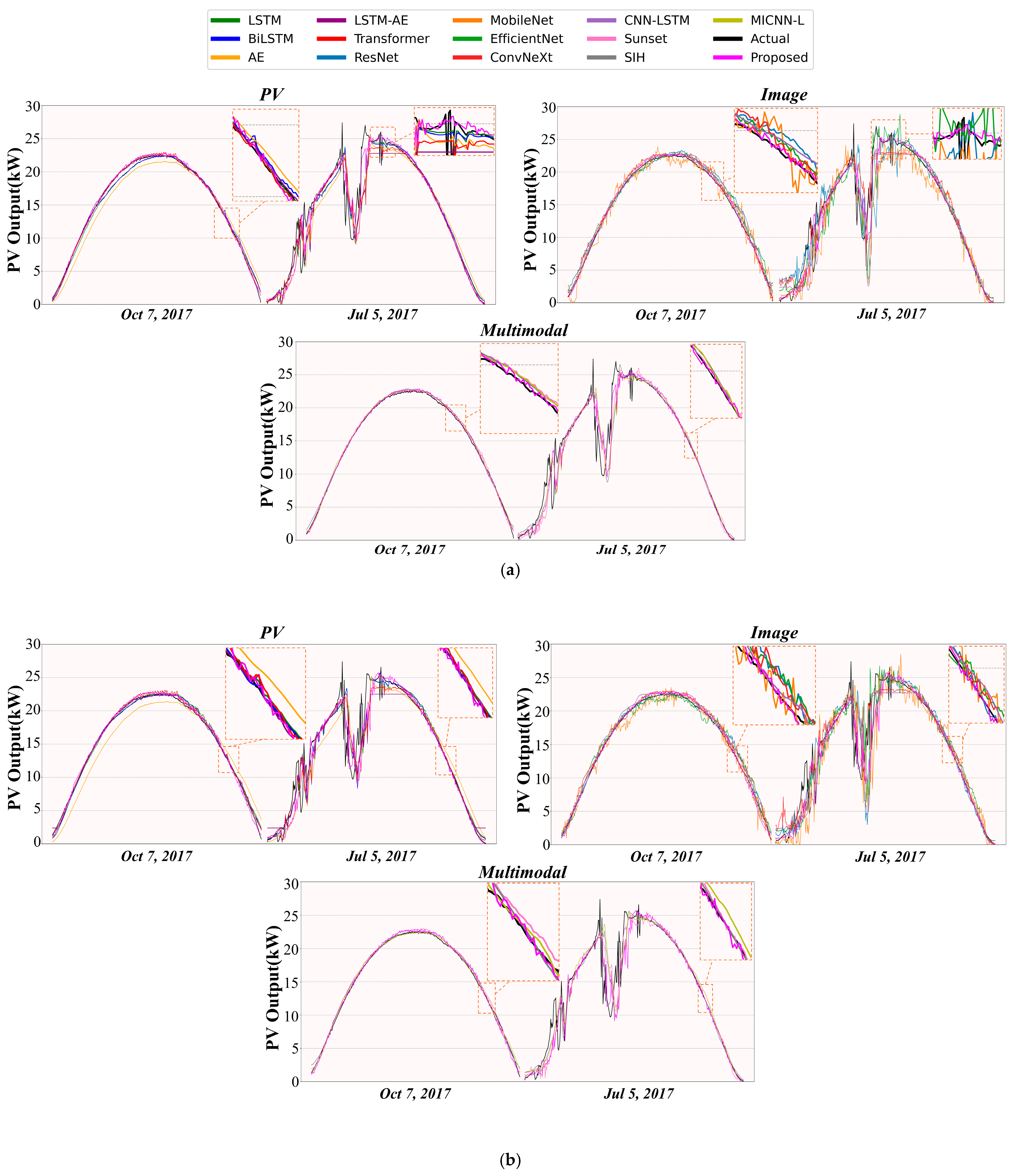
6.1. Comparison of the Proposed Model with the Benchmark Models

Considering the various benchmark models presented in Section 5.2, this study adequately compared them with the models in this study from three aspects: performance comparison under overall performance conditions, performance comparison under different weather conditions, and model uncertainty analysis.

6.1.1. Overall Performance of the Proposed Model and Benchmark Models Comparisons

Table 2. Comparison results of the proposed model with different modal models in the 10 min prediction range.

Stage	Model	$\mathbf{MAE} \left(\mathbf{kW}\right) \downarrow$	$\mathbf{RMSE} \left(\mathbf{kW}\right) \downarrow$	$\mathbf{Forecast} \mathbf{Skill} (\%) \uparrow$
Only PV	LSTM [11]	1.315	2.786	10.91
	Bi-LSTM [10]	1.286	2.78	11.12
	AE [52]	1.861	3.02	3.44
	LSTM-AE [53]	1.281	2.781	11.09
	Transformer [54]	1.244	2.713	13.25
Only image	ResNet [55]	1.438	2.641	15.14
	MobileNet [56]	1.65	2.841	9.16
	EfficientNet [57]	1.533	2.656	15.09
	ConvNeXt [58]	1.526	2.733	12.62
	CNN-LSTM [59]	1.678	2.826	9.64
Multimodal	Sunset [42]	1.219	2.539	18.81
	SIH [20]	1.217	2.646	15.41
	MICNN-L [60]	1.218	2.582	17.45
	Proposed	1.099	2.48	20.72

The upward arrows (↑) indicate that higher values are better, while the downward arrows (↓) indicate that lower values are better.

,

Table 3. Comparison results of the proposed model with different modal models in the 15 min prediction range.

Stage	Model	$\mathbf{MAE} \left(\mathbf{kW}\right) \downarrow$	$\mathbf{RMSE} \left(\mathbf{kW}\right) \downarrow$	$\mathbf{Forecast} \mathbf{Skill} (\%) \uparrow$
Only PV	LSTM [11]	1.451	2.887	10.66
	Bi-LSTM [10]	1.45	2.9	10.25
	AE [52]	2.118	3.21	0.67
	LSTM-AE [53]	1.463	2.884	10.75
	Transformer [54]	1.391	2.802	13.28
Only image	ResNet [55]	1.484	2.633	18.52
	MobileNet [56]	1.754	2.978	7.83
	EfficientNet [57]	1.566	2.74	15.22
	ConvNeXt [58]	1.574	2.763	14.5
	CNN-LSTM [59]	1.705	2.894	10.44
Multimodal	Sunset [42]	1.333	2.592	19.78
	SIH [20]	1.339	2.684	16.94
	MICNN-L [60]	1.328	2.634	18.49
	Proposed	1.176	2.45	24.2

The upward arrows (↑) indicate that higher values are better, while the downward arrows (↓) indicate that lower values are better.

and

Table 4. Comparison results of the proposed model with different modal models in the 20 min prediction range.

Stage	Model	$\mathbf{MAE} \left(\mathbf{kW}\right) \downarrow$	$\mathbf{RMSE} \left(\mathbf{kW}\right) \downarrow$	$\mathbf{Forecast} \mathbf{Skill} (\%) \uparrow$
Only PV	LSTM [11]	1.636	3.107	9.4
	Bi-LSTM [10]	1.626	3.088	9.95
	AE [52]	2.373	3.484	−1.59
	LSTM-AE [53]	1.605	3.062	10.7
	Transformer [54]	1.539	2.982	13.05
Only image	ResNet [55]	1.63	2.823	17.68
	MobileNet [56]	1.869	3.068	10.54
	EfficientNet [57]	1.676	2.917	14.95
	ConvNeXt [58]	1.76	2.918	14.92
	CNN-LSTM [59]	1.82	3.028	11.7
Multimodal	Sunset [42]	1.4	2.7	21.27
	SIH [20]	1.459	2.815	17.91
	MICNN-L [60]	1.443	2.752	19.76
	Proposed	1.308	2.618	23.67

The upward arrows (↑) indicate that higher values are better, while the downward arrows (↓) indicate that lower values are better.

present the comparison results between the proposed model and the benchmark models, reflecting their overall performance. Among the time-series models, LSTM and Bi-LSTM performed well in the short-term forecasts of 10 and 15 min due to their gating mechanisms, which could effectively capture the time dependence, but they lagged behind LSTM-AE in the progressively longer time steps. It was not difficult to see that AE alone showed high errors, which suggests that there are limitations in its ability to capture the information of the time series. In contrast, however, LSTM-AE combined both strengths and performed well at all time steps. The transformer model, which utilizes a self-attentive mechanism to capture global temporal patterns, showed a sustained advantage, with the MAE decreasing compared to the other models by 2.89–33.2%, 4.1–34.3%, and 4.1–35.1% at 10 min, 15 min, and 20 min, respectively, highlighting its ability to effectively handle complex time-series data. However, when applying the proposed method, it achieved the best prediction accuracy in all metrics, proving its robustness and efficiency in time-series forecasting compared to all unimodal methods.

In the comparison of the image models, there were substantial disparities in the performance of several convolutional neural networks. EfficientNet performed well in all prediction steps and significantly outperformed the other convolutional networks. This suggests that EfficientNet’s modern architectural design of deeply separable convolution and squeeze-and-excitation mechanism makes it more suitable for capturing complex image features such as cloud motion. In contrast, ConvNeXt and MobileNet, despite their advantages in model efficiency, performed poorly in prediction accuracy, indicating their lack of ability in complex feature extraction. CNN-LSTM, despite combining spatial and temporal feature extraction, still had a higher overall error than ConvNeXt and other more modern convolutional models, while ResNet, as a classic residual network architecture, performed well in image feature extraction, with RMSEs that were lower than those of the other models by 0.6–33.2% for 10, 15, and 20 min, respectivelyIn terms of FS, ResNet achieves improvements of0.6–7%, 3.9–11.6% and 3.2–8% at 10 min, 15 min and 20 min, respectively), but was still too different in terms of error when compared to the proposed model.

In the comparison of the same multimodal models, sunset, SIH, and MICNN-L showed different feature extraction and fusion strategies. SIH and MICNN-L performed well in the short-term prediction, which shows their ability to handle multimodal data, but the error increased with the increase in the prediction step, which was not as good as sunset, which performed well in the short-term prediction, especially in the 15-min prediction with MAEs of 1.333 kW and 1.328 kW, respectively. Sunset performed very well in short-term prediction and also maintained low errors in 15-min and 20-min prediction, which was significantly lower than that of SIH and MICNN-L, indicating that its multimodal fusion strategy has high accuracy in short-term prediction tasks. In contrast, the multimodal model proposed in this paper significantly improved the prediction performance through the innovative ACMCA mechanism. In the 15-min prediction, the MAE of this paper’s model was 1.176 kW, which was much lower than that of all the other models. Concurrently, the model presented in this research had the highest FS throughout all forecasting stages, with a value of 24.2% in 15-min forecasting, which was much better than the other models. Overall, through the detailed comparative analysis of different modalities, the multimodal fusion model proposed in this paper had a significant advantage in capturing the complementary information of time-series data and image data and performed well in all kinds of prediction tasks, showing the strongest robustness and prediction accuracy.

Aside from the error analysis based on performance metrics, visual comparisons were conducted to assess the predictive performance of the proposed model against benchmarks on two representative days (sunny on 7 October 2017, and cloudy on 5 July 2017), with data sampled every 2 min. Figure 4a–c illustrates the actual and predicted PV outputs. Among the time-series models, AE, LSTM, LSTM-AE, and BiLSTM performed well in the short-term (first 10 min), but faced declines in accuracy over more extended periods, especially during rapid cloud changes, due to error accumulation in sequential inference. While the transformer model improved the performance with a self-attention mechanism, it encountered confusion and redundancy by using all inputs, leading to less efficient feature extraction. Overall, the proposed model demonstrated superior prediction accuracy across all conditions.

In comparing the image models, MobileNet and CNN-LSTM generally performed well in short-term predictions, but their accuracy dropped significantly during periods of complex cloud movement, showing noticeable deviations from the actual values. ConvNeXt and EfficientNet achieved better results under complex weather conditions due to deeper feature extraction, but they still struggled to fully adapt to rapid weather changes, with notable prediction fluctuations. Although ResNet could capture the actual values more accurately during severe fluctuations, its overall performance still lagged behind the proposed model, which maintained stable accuracy under all conditions.

The multimodal model aims to leverage both sky images and historical PV data to enhance prediction accuracy. As shown in the results, models like MICNN-L, SIH, and sunset improve performance under certain complex weather conditions compared to unimodal models. However, they still struggle to capture all of the critical features in scenarios such as fast-moving clouds. In contrast, the proposed model consistently performed well across all time steps, with significantly lower curve deviations than other multimodal models, regardless of the weather conditions. Particularly at the 10-min time step, its predictions almost perfectly aligned with the actual data, demonstrating its strong fusion capability for multimodal data and adaptability to complex scenarios.

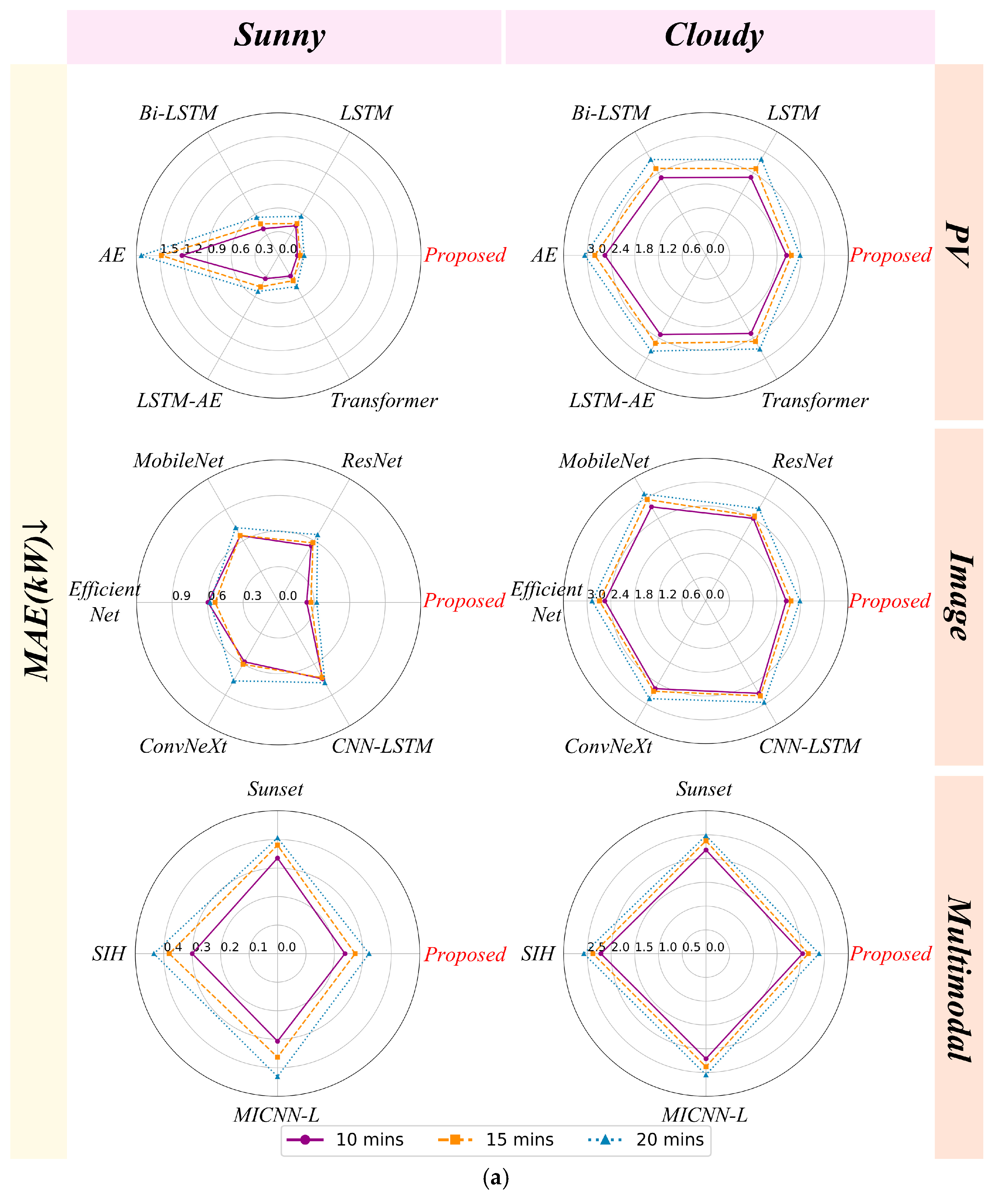
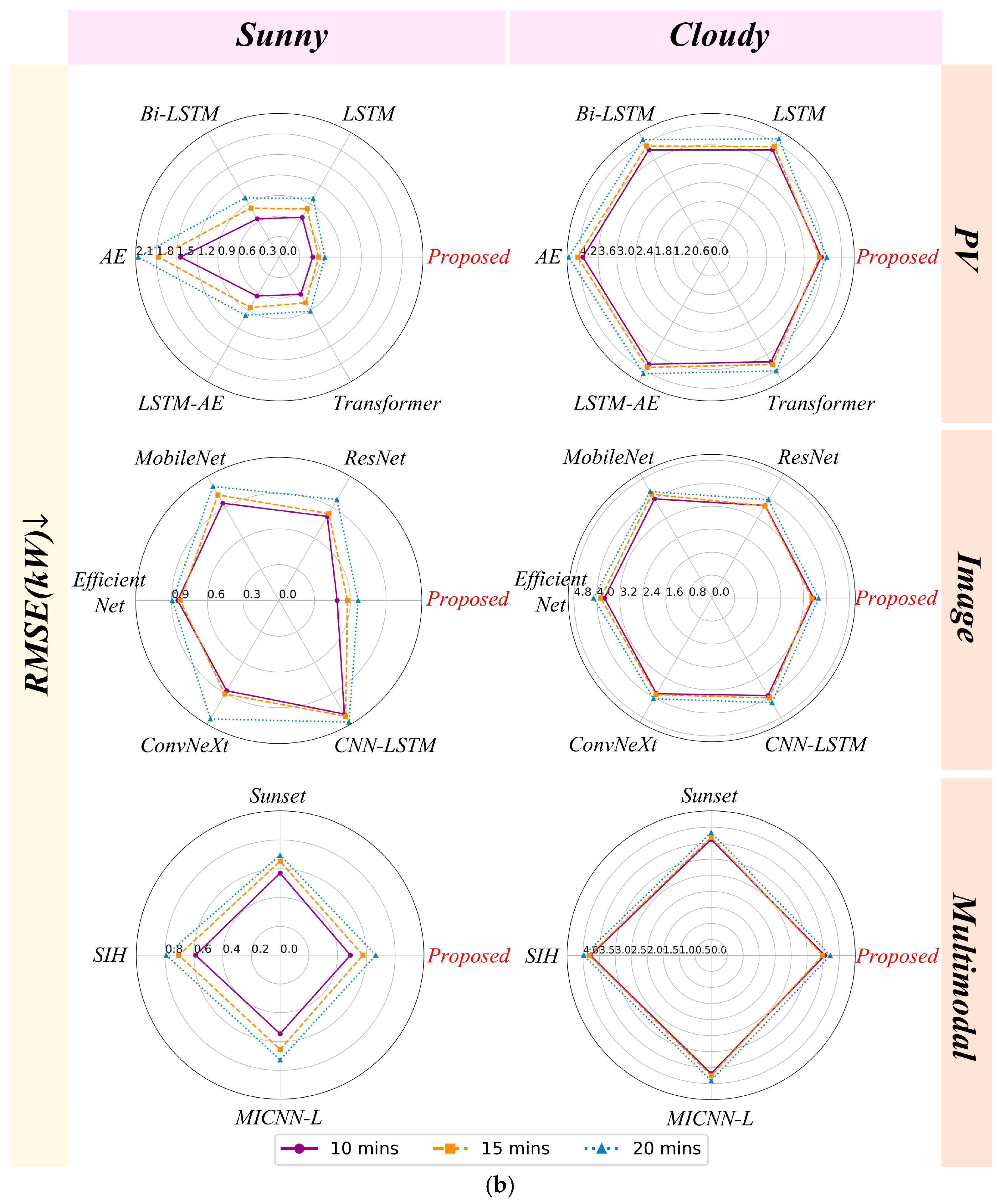
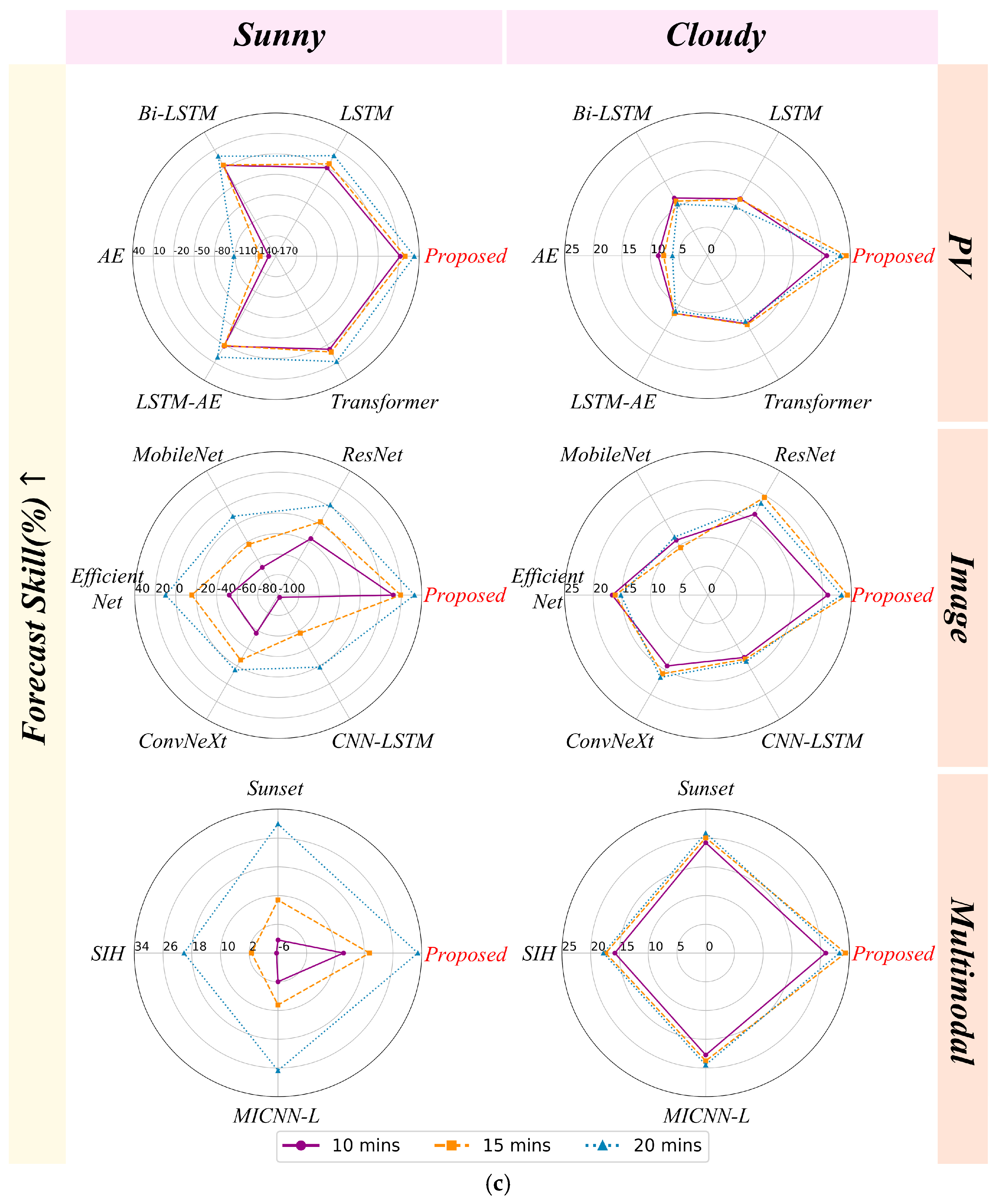
6.1.2. Comparison of Different Weather Conditions

This study evaluated the prediction error and curve fitting while validating the performance of the proposed model alongside three comparative models across multiple metrics under differing weather circumstances, categorized as sunny and overcast based on sky images. The results of the different mode comparisons are shown in Figure 5a–c. Forecast errors are generally lower under sunny conditions, while performance varies more under cloudy conditions. The proposed multimodal model demonstrated the best accuracy across all forecast ranges in both scenarios. Sudden changes in PV output under cloudy conditions are mainly due to cloud motion. The proposed model achieved MAE values of 2.037–2.16–2.384 kW, RMSE of 3.547–3.49–3.721 kW, and FS of 20.87–24.32–23.27%, outperforming other models. While all multimodal models performed better than unimodal models, Sunset showed competitive results with an MAE of 2.181–2.373–2.483 kW, RMSE of 3.621–3.685–3.836 kW, and FS of 19.21–20.08–20.9%. The results suggest that historical time-series data and sky images were individually effective for sunny and cloudy conditions but still fell short of the overall performance of Sunset and the proposed model. The validation confirms that the innovative ACMCA mechanism has stronger predictive ability and adaptability with multimodal data, effectively handling varying conditions and maintaining reliability across different weather scenarios.

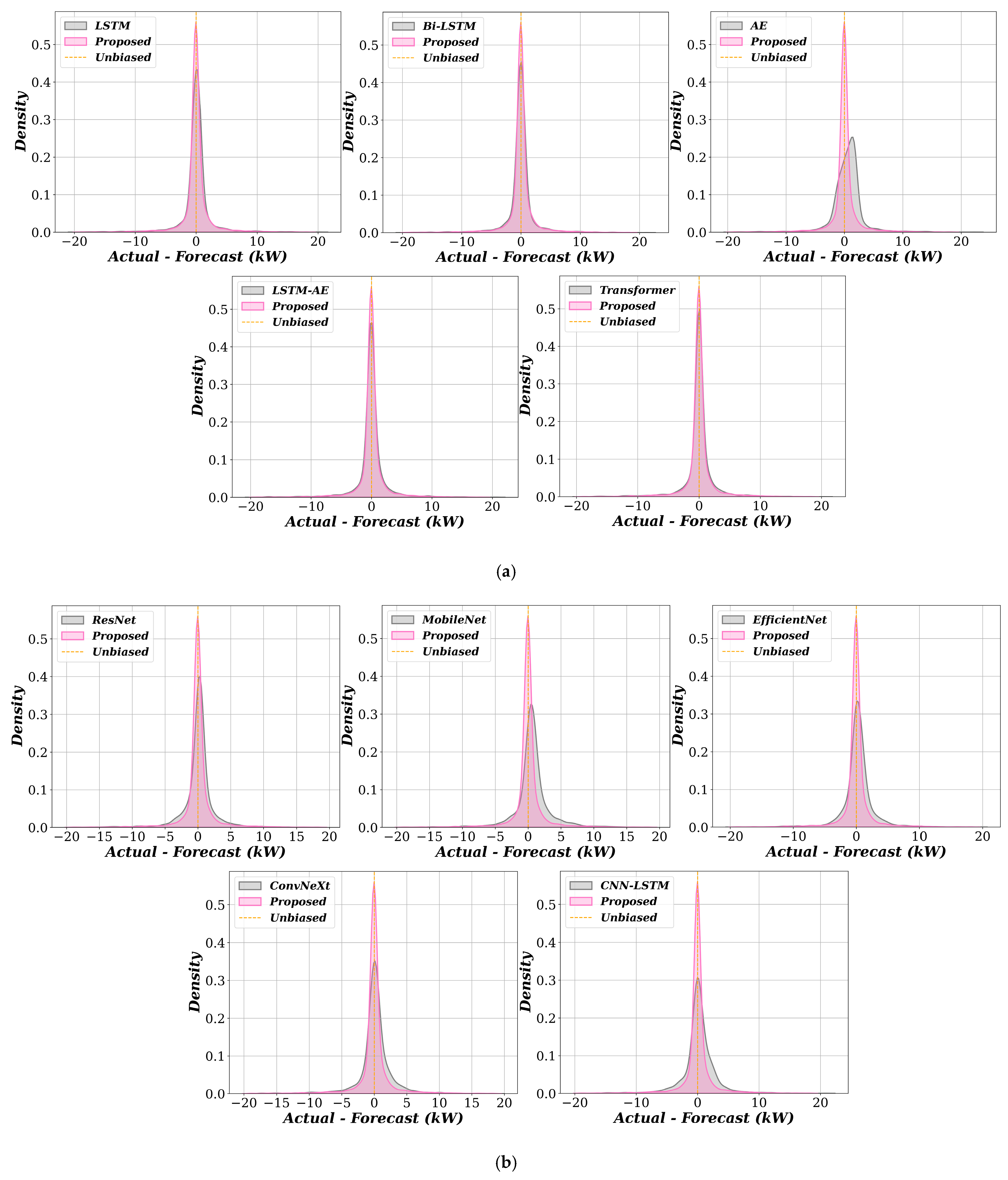
6.1.3. Uncertainty Analysis of the Proposed Model and the Benchmark Model

In addition to forecasting accuracy, the robustness of these methods can be effectively assessed through uncertainty analysis. Figure 6a–c illustrates the distribution of prediction errors across different models. The prediction errors of the proposed model were predominantly centered around 0. Consistent with the previous analysis of model prediction accuracy, AE, CNN-LSTM, and MobileNet demonstrated suboptimal performance, as the error distribution revealed that the lowest density was near zero and the most significant departure from the ideal outcome. SIH showed some improvement over transformer and MICNN-L. In addition, sunset was the second-best method, with an abundance near zero second only to the proposed model. Consequently, the uncertainty analysis aligned with the previously mentioned error and accuracy analyses. The proposed model guaranteed the most constrained distribution along the error axis, hence exhibiting the optimal resilience and stability.

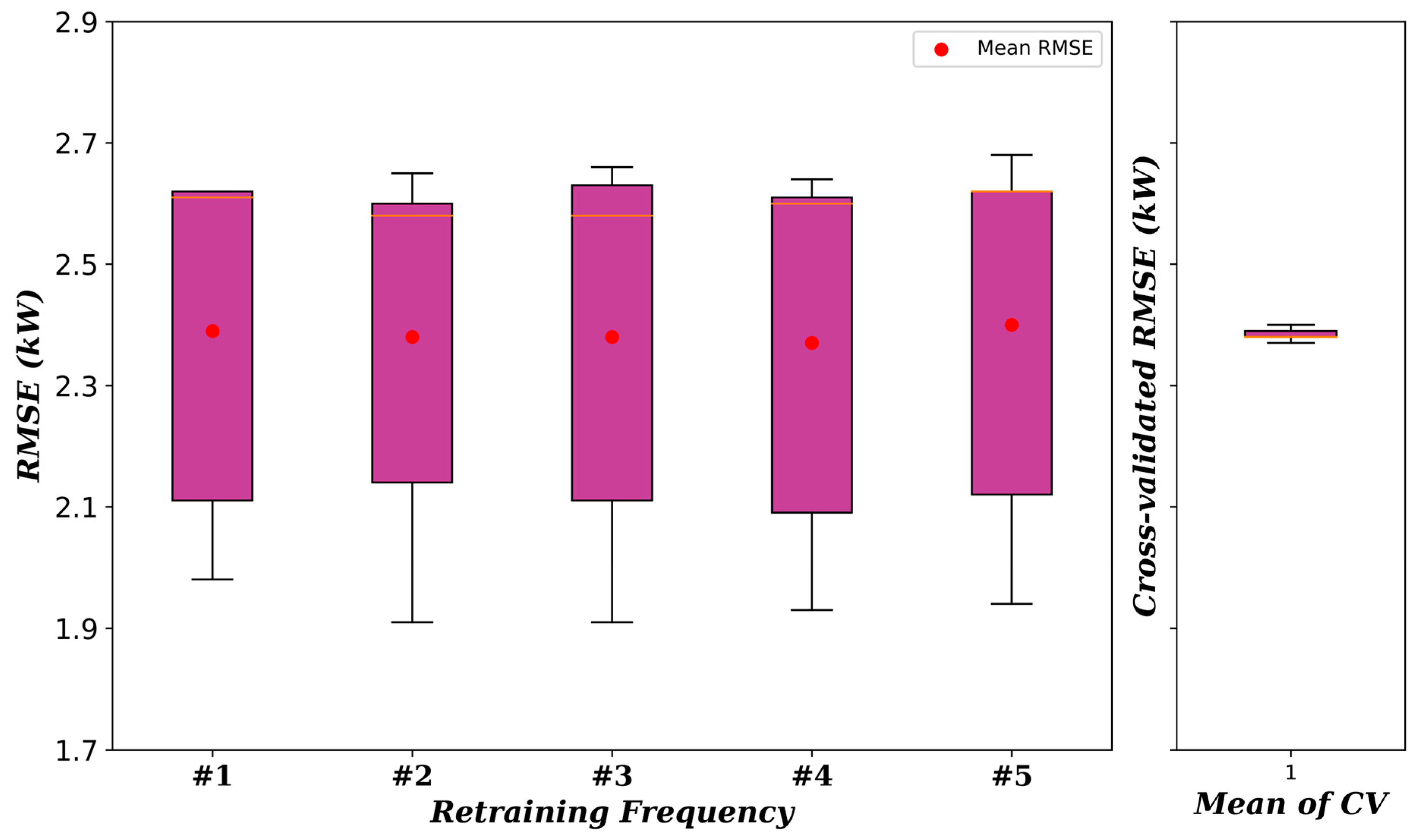
6.2. The Uncertainty in Mean RMSE of the Proposed Model

Considering the random characteristics of the optimizer, training the same model on identical datasets can result in slight performance variations. To verify whether the proposed model’s advantages were genuine or random, we quantified the training uncertainty through 25 runs, organized into fivefold cross-validation (CV), with each set using different random initializations. As shown in Figure 7, the RMSE on the validation set varied across folds within each CV, sometimes nearing 2.7 kW, mainly due to dataset heterogeneity, where cloudy days are more challenging to predict than sunny days. However, the right panel highlights the model’s robustness, as the average RMSE across CVs remained stable with a minimal standard variation of 0.011 kW, affirming the stability of the ADAM optimizer.

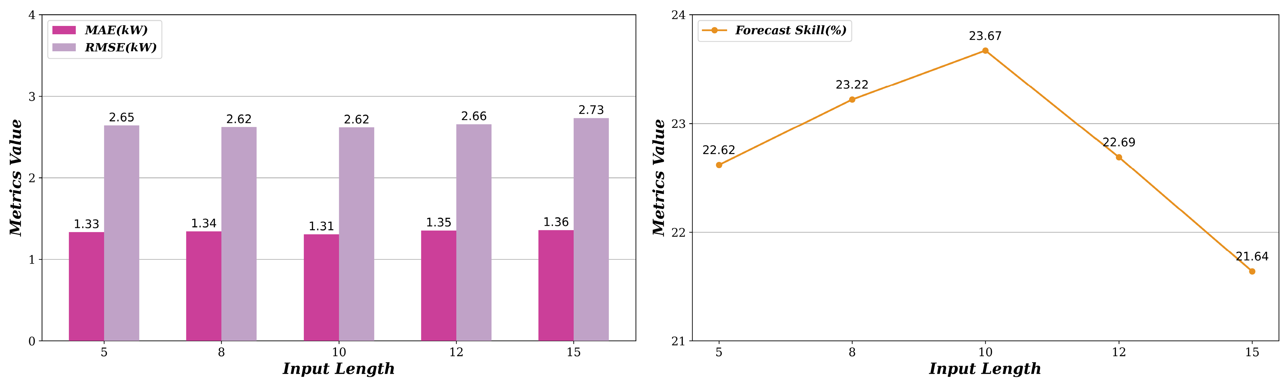
6.3. Sensitivity Analysis of Input Sequence Length

In general, extending the sky image sequence and historical PV data provides richer features for PV power forecasting. However, as the lag increases, the relevance of the sky images and historical PV data to current conditions may diminish. Conversely, shorter sequence data do not adequately capture the corresponding features. Consequently, inputting excessively long or short sequences may diminish the efficacy of feature extraction. We verified the effect of five different input sequence lengths for different metrics. Figure 8 illustrates the ideal configuration of input sequence length is 10-min historical sequence data (11 lags), which had an FS 1.9–9.4% higher than the other results.

6.4. Ablation Experiments for the Proposed Model

To elucidate the function of each component in the proposed multimodal model, this section presents the ablation results for different modules across various prediction ranges. “Proposed without PV stage” denotes removing the PV feature autocorrelation learning stage, replaced by a fully connected layer, leaving only the image feature extraction and fusion components. “Proposed without image stage” refers to eliminating the feature encoder for learning cloud motion, replaced by a linear layer, retaining only the PV feature extraction and fusion parts. “Proposed without fusion stage” indicates the absence of the cross-modal feature fusion, where the PV and image features are directly spliced.

The ablation results are shown in

Table 5. Experimental results of ablation of the proposed model in the 10 min prediction range.

Model	$\mathbf{MAE} \left(\mathbf{kW}\right) \downarrow$	$\mathbf{RMSE} \left(\mathbf{kW}\right) \downarrow$	$\mathbf{Forecast} \mathbf{Skill} (\%) \uparrow$
Proposed without PV stage	1.143	2.528	19.17
Proposed without image stage	1.251	2.572	17.77
Proposed without fusion stage	1.135	2.537	18.88
Proposed	1.099	2.48	20.72

The upward arrows (↑) indicate that higher values are better, while the downward arrows (↓) indicate that lower values are better.

,

Table 6. Experimental results of ablation of the proposed model in the 15 min prediction range.

Model	$\mathbf{MAE} \left(\mathbf{kW}\right) \downarrow$	$\mathbf{RMSE} \left(\mathbf{kW}\right) \downarrow$	$\mathbf{Forecast} \mathbf{Skill} (\%) \uparrow$
Proposed without PV stage	1.251	2.507	22.42
Proposed without image stage	1.371	2.625	18.78
Proposed without fusion stage	1.22	2.543	21.3
Proposed	1.176	2.45	24.2

The upward arrows (↑) indicate that higher values are better, while the downward arrows (↓) indicate that lower values are better.

and

Table 7. Experimental results of ablation of the proposed model in the 20 min prediction range.

Model	$\mathbf{MAE} \left(\mathbf{kW}\right) \downarrow$	$\mathbf{RMSE} \left(\mathbf{kW}\right) \downarrow$	$\mathbf{Forecast} \mathbf{Skill} (\%) \uparrow$
Proposed without PV stage	1.388	2.672	22.1
Proposed without image stage	1.476	2.769	19.25
Proposed without fusion stage	1.322	2.649	22.76
Proposed	1.308	2.618	23.67

The upward arrows (↑) indicate that higher values are better, while the downward arrows (↓) indicate that lower values are better.

. Removing the PV feature autocorrelation learning stage reduces the model’s ability to capture the dynamic characteristics of PV power generation, leading to a significant drop in accuracy. Eliminating the image feature encoder impairs the model’s ability to capture changes in irradiance due to cloud motion, especially during fluctuating weather, affecting the prediction accuracy. Finally, bypassing the cross-modal feature fusion results in a less effective integration of the PV and image features, as simple feature splicing fails to exploit deep correlations, causing a slight decrease in the overall accuracy.

6.5. Sensitivity Analysis of Input Degradation and Missingness

To evaluate the robustness of the proposed model, we conducted sensitivity experiments by degrading the quality of the input data and simulating data missingness. Two sets of experiments were performed: adding Gaussian noise to the input data (degradation) and introducing random data dropout to simulate missing information (missingness). The results are presented in

Table 8. Degradation and missingness experiments for 10-min prediction.

Experiment Type	Noise/Dropout Rate	$\mathbf{MAE} \left(\mathbf{kW}\right) \downarrow$	$\mathbf{RMSE} \left(\mathbf{kW}\right) \downarrow$	$\mathbf{Forecast} \mathbf{Skill} (\%) \uparrow$
Proposed	0%	1.099	2.480	20.72
Degradation	1%	1.097	2.480	20.73
	5%	1.095	2.482	20.66
	10%	1.100	2.481	20.70
Missingness	1%	1.110	2.482	20.64
	3%	1.137	2.493	20.30
	5%	1.171	2.498	20.12

The upward arrows (↑) indicate that higher values are better, while the downward arrows (↓) indicate that lower values are better.

,

Table 9. Degradation and missingness experiments for 15-min prediction.

Experiment Type	Noise/Dropout Rate	$\mathbf{MAE} \left(\mathbf{kW}\right) \downarrow$	$\mathbf{RMSE} \left(\mathbf{kW}\right) \downarrow$	$\mathbf{Forecast} \mathbf{Skill} (\%) \uparrow$
Proposed	0%	1.176	2.450	24.20
Degradation	1%	1.179	2.453	24.09
	5%	1.181	2.456	24.00
	10%	1.182	2.459	23.94
Missingness	1%	1.192	2.452	24.13
	3%	1.224	2.463	23.77
	5%	1.270	2.494	22.81

The upward arrows (↑) indicate that higher values are better, while the downward arrows (↓) indicate that lower values are better.

and

Table 10. Degradation and missingness experiments for 20-min prediction.

Experiment Type	Noise/Dropout Rate	$\mathbf{MAE} \left(\mathbf{kW}\right) \downarrow$	$\mathbf{RMSE} \left(\mathbf{kW}\right) \downarrow$	$\mathbf{Forecast} \mathbf{Skill} (\%) \uparrow$
Proposed	0%	1.308	2.618	23.67
Degradation	1%	1.312	2.615	23.76
	5%	1.315	2.623	23.54
	10%	1.308	2.611	23.89
Missingness	1%	1.318	2.613	23.80
	3%	1.360	2.618	23.66
	5%	1.401	2.639	23.06

The upward arrows (↑) indicate that higher values are better, while the downward arrows (↓) indicate that lower values are better.

for the 10-min, 15-min, and 20-min prediction horizons, respectively.

In the degradation experiments, Gaussian noise with different standard deviations was added to the input data. As shown in the tables, the model’s performance metrics exhibited only slight variations across all noise levels. For instance, for the 10-min prediction horizon, the RMSE increased marginally from 2.480 kW to 2.481 kW under 10% noise, and the forecast skill decreased from 20.72% to 20.70%. These results indicate that the proposed model effectively mitigated the impact of input noise and demonstrated strong robustness in handling degraded input data.

For the missingness experiments, random data dropout was introduced at rates of 1%, 3%, and 5%. Similarly, the results revealed minimal performance degradation. For the 20-min prediction horizon, the RMSE increased slightly from 2.618 kW to 2.639 kW at 5% dropout, while the forecast skill decreased marginally from 23.67% to 23.06%. These findings highlight the model’s ability to tolerate missing input information while maintaining a high level of accuracy.

7. Conclusions

This paper proposed an end-to-end multimodal prediction framework based on an attention mechanism to address the challenges of PV power forecasting in VPPs. The volatility and uncertainty of PV generation, especially under complex weather conditions, complicate efficient VPP management and grid stability, which traditional unimodal methods struggle to handle. By integrating historical PV time-series data and sky images with the ACMCA mechanism, the proposed model adaptively mines correlations between different modalities, enhancing prediction accuracy and robustness, thus providing reliable support for VPP operations. Extensive experiments demonstrated that the proposed model exceled across various prediction horizons and weather conditions. Specifically, in the 20-min forecast, it achieved a 24.2% accuracy across all scenarios, rising to 24.32% in cloudy conditions, thus outperforming the traditional unimodal and other multimodal methods by 4.42% and 4.24%, respectively. The model consistently surpassed the baseline methods across all metrics, showing strong adaptability and robustness, particularly in complex weather scenarios like cloudy and rainy days. From the numerical results, the subsequent conclusions can be derived.

• The multimodal learning prediction framework proposed in this paper effectively captures dynamic changes in PV power generation by integrating time-series data and image data. Experimental results demonstrated strong prediction performance across various weather conditions, significantly enhancing the stability and accuracy of VPPs in short-term power forecasting.
• The designed ACMCA mechanism enables the deep fusion of multimodal features by adaptively learning correlations between temporal and image data, enhancing the complementarity of different modalities. Compared to traditional baseline models, ACMCA showed greater robustness in handling complex weather conditions (e.g., cloudy), offering a more reliable basis for PV power forecasting.
• Extensive experiments showed that the proposed method surpassed the existing unimodal and other multimodal approaches in prediction error, accuracy, and efficiency. Particularly in multimodal data applications, it consistently outperformed traditional baseline models across different time periods and complex weather conditions, validating its practical value for VPP management.

While the proposed multimodal framework has shown promising results in short-term PV forecasting, there is still room for optimization. Future work could integrate more data sources, such as weather forecasts or satellite images, to improve model generalization. This approach can be applied to VPP facilities to predict the PV output within 10 to 20 min, aiding in efficient VPP management and power dispatch optimization when used with all-day imagers in PV plants.

References

1. REN21. Renewables 2018 Global Status Report; REN21 Secretariat: Paris, France, 2018; ISBN 978-3-9818911-3-3. Available online: https://www.ren21.net/gsr-2018/ (accessed on 12 December 2024).
2. Cozzi, L.; Gould, T.; Bouckart, S.; Crow, D.; Kim, T.-Y.; McGlade, C.; Olejarnik, P.; Wanner, B.; Wetzel, D. World energy outlook 2020. Energy 2020, 2019, 30. [Google Scholar]
3. Shahsavari, A.; Akbari, M. Potential of solar energy in developing countries for reducing energy-related emissions. Renew. Sustain. Energy Rev. 2018, 90, 275–291. [Google Scholar] [CrossRef]
4. Ding, M.; Xu, Z.; Wang, W.; Wang, X.; Song, Y.; Chen, D. A review on China׳ s large-scale PV integration: Progress, challenges and recommendations. Renew. Sustain. Energy Rev. 2016, 53, 639–652. [Google Scholar] [CrossRef]
5. Marquez, R.; Coimbra, C.F.M. Intra-hour DNI forecasting based on cloud tracking image analysis. Sol. Energy 2013, 91, 327–336. [Google Scholar] [CrossRef]
6. Quesada-Ruiz, S.; Chu, Y.; Tovar-Pescador, J.; Pedro, H.T.; Coimbra, C.F. Cloud-tracking methodology for intra-hour DNI forecasting. Sol. Energy 2014, 102, 267–275. [Google Scholar] [CrossRef]
7. Mahmud, K.; Khan, B.; Ravishankar, J.; Ahmadi, A.; Siano, P. An internet of energy framework with distributed energy resources, prosumers and small-scale virtual power plants: An overview. Renew. Sustain. Energy Rev. 2020, 127, 109840. [Google Scholar] [CrossRef]
8. Jakoplić, A.; Franković, D.; Kirinčić, V.; Plavšić, T. Benefits of short-term photovoltaic power production forecasting to the power system. Optim. Eng. 2021, 22, 9–27. [Google Scholar] [CrossRef]
9. Radzi, M.; Liyana, P.N.; Akhter, M.N.; Mekhilef, S.; Shah, N.M. Review on the application of photovoltaic forecasting using machine learning for very short-to long-term forecasting. Sustainability 2023, 15, 2942. [Google Scholar] [CrossRef]
10. Chen, Y.; Bhutta, M.S.; Abubakar, M.; Xiao, D.; Almasoudi, F.M.; Naeem, H.; Faheem, M. Evaluation of machine learning models for smart grid parameters: Performance analysis of ARIMA and Bi-LSTM. Sustainability 2023, 15, 8555. [Google Scholar] [CrossRef]
11. Kuo, W.-C.; Chen, C.-H.; Hua, S.-H.; Wang, C.-C. Assessment of different deep learning methods of power generation forecasting for solar PV system. Appl. Sci. 2022, 12, 7529. [Google Scholar] [CrossRef]
12. Chen, C.; Duan, S.; Cai, T.; Liu, B. Online 24-h solar power forecasting based on weather type classification using artificial neural network. Sol. Energy 2011, 85, 2856–2870. [Google Scholar] [CrossRef]
13. Chu, Y.; Pedro, H.T.C.; Coimbra, C.F.M. Hybrid intra-hour DNI forecasts with sky image processing enhanced by stochastic learning. Sol. Energy 2013, 98, 592–603. [Google Scholar] [CrossRef]
14. Nie, Y.; Sun, Y.; Chen, Y.; Orsini, R.; Brandt, A. PV power output prediction from sky images using convolutional neural network: The comparison of sky-condition-specific sub-models and an end-to-end model. J. Renew. Sustain. Energy 2020, 12, 046101. [Google Scholar] [CrossRef]
15. Ahmed, R.; Sreeram, V.; Mishra, Y.; Arif, M.D. A review and evaluation of the state-of-the-art in PV solar power forecasting: Techniques and optimization. Renew. Sustain. Energy Rev. 2020, 124, 109792. [Google Scholar] [CrossRef]
16. Shi, J.; Lee, W.-J.; Liu, Y.; Yang, Y.; Wang, P. Forecasting power output of photovoltaic systems based on weather classification and support vector machines. IEEE Trans. Ind. Appl. 2012, 48, 1064–1069. [Google Scholar] [CrossRef]
17. Haputhanthri, D.; De Silva, D.; Sierla, S.; Alahakoon, D.; Nawaratne, R.; Jennings, R.; Vyatkin, V. Solar irradiance nowcasting for virtual power plants using multimodal long short-term memory networks. Front. Energy Res. 2021, 9, 722212. [Google Scholar] [CrossRef]
18. Zuo, H.-M.; Qiu, J.; Li, F.-F. Ultra-short-term forecasting of global horizontal irradiance (GHI) integrating all-sky images and historical sequences. J. Renew. Sustain. Energy 2023, 15, 0163759. [Google Scholar] [CrossRef]
19. Li, J.; Hong, D.; Gao, L.; Yao, J.; Zheng, K.; Zhang, B.; Chanussot, J. Deep learning in multimodal remote sensing data fusion: A comprehensive review. Int. J. Appl. Earth Obs. Geoinf. 2022, 112, 102926. [Google Scholar] [CrossRef]
20. Kong, W.; Jia, Y.; Dong, Z.Y.; Meng, K.; Chai, S. Hybrid approaches based on deep whole-sky-image learning to photovoltaic generation forecasting. Appl. Energy 2020, 280, 115875. [Google Scholar] [CrossRef]
21. Wan, C.; Zhao, J.; Song, Y.; Xu, Z.; Lin, J.; Hu, Z. Photovoltaic and solar power forecasting for smart grid energy management. CSEE J. Power Energy Syst. 2015, 1, 38–46. [Google Scholar] [CrossRef]
22. Lipperheide, M.; Bosch, J.L.; Kleissl, J. Embedded nowcasting method using cloud speed persistence for a photovoltaic power plant. Sol. Energy 2015, 112, 232–238. [Google Scholar] [CrossRef]
23. Sobri, S.; Koohi-Kamali, S.; Rahim, N.A. Solar photovoltaic generation forecasting methods: A review. Energy Convers. Manag. 2018, 156, 459–497. [Google Scholar] [CrossRef]
24. Sreekumar, S.; Bhakar, R. Solar power prediction models: Classification based on time horizon, input, output and application. In Proceedings of the 2018 International Conference on Inventive Research in Computing Applications (ICIRCA), Coimbatore, India, 11–12 July 2018. [Google Scholar] [CrossRef]
25. Dong, J.; Olama, M.M.; Kuruganti, T.; Melin, A.M.; Djouadi, S.M.; Zhang, Y.; Xue, Y. Novel stochastic methods to predict short-term solar radiation and photovoltaic power. Renew. Energy 2020, 145, 333–346. [Google Scholar] [CrossRef]
26. Sheng, H.; Xiao, J.; Cheng, Y.; Ni, Q.; Wang, S. Short-term solar power forecasting based on weighted Gaussian process regression. IEEE Trans. Ind. Electron. 2017, 65, 300–308. [Google Scholar] [CrossRef]
27. Feng, C.; Zhang, J. Hourly-similarity based solar forecasting using multi-model machine learning blending. In Proceedings of the 2018 IEEE Power & Energy Society General Meeting (PESGM), Portland, OR, USA, 5–10 August 2018. [Google Scholar] [CrossRef]
28. Kong, W.; Dong, Z.-Y.; Jia, Y.; Hill, D.J.; Xu, Y.; Zhang, Y. Short-term residential load forecasting based on LSTM recurrent neural network. IEEE Trans. Smart Grid 2017, 10, 841–851. [Google Scholar] [CrossRef]
29. Ren, S.; Hu, W.; Bradbury, K.; Harrison-Atlas, D.; Valeri, L.M.; Murray, B.; Malof, J.M. Automated extraction of energy systems information from remotely sensed data: A review and analysis. Appl. Energy 2022, 326, 119876. [Google Scholar] [CrossRef]
30. Cheng, L.; Zang, H.; Wei, Z.; Ding, T.; Xu, R.; Sun, G. Short-term solar power prediction learning directly from satellite images with regions of interest. IEEE Trans. Sustain. Energy 2021, 13, 629–639. [Google Scholar] [CrossRef]
31. Feng, C.; Zhang, J. SolarNet: A sky image-based deep convolutional neural network for intra-hour solar forecasting. Sol. Energy 2020, 204, 71–78. [Google Scholar] [CrossRef]
32. Niu, T.; Li, J.; Wei, W.; Yue, H. A hybrid deep learning framework integrating feature selection and transfer learning for multi-step global horizontal irradiation forecasting. Appl. Energy 2022, 326, 119964. [Google Scholar] [CrossRef]
33. Ronneberger, O.; Fischer, P.; Brox, T. U-net: Convolutional networks for biomedical image segmentation. In Proceedings of the Medical Image Computing and Computer-Assisted Intervention–MICCAI 2015: 18th International Conference, Munich, Germany, 5–9 October 2015. proceedings, part III 18. [Google Scholar] [CrossRef]
34. Yao, T.; Wang, J.; Wu, H.; Zhang, P.; Li, S.; Xu, K.; Liu, X.; Chi, X. Intra-hour photovoltaic generation forecasting based on multi-source data and deep learning methods. IEEE Trans. Sustain. Energy 2021, 13, 607–618. [Google Scholar] [CrossRef]
35. Lotter, W.; Kreiman, G.; Cox, D. Deep predictive coding networks for video prediction and unsupervised learning. arXiv 2016, arXiv:1605.08104. [Google Scholar]
36. Lin, Z.; Li, M.; Zheng, Z.; Cheng, Y.; Yuan, C. Self-attention convlstm for spatiotemporal prediction. Proc. AAAI Conf. Artif. Intell. 2020, 34, 11531–11538. [Google Scholar] [CrossRef]
37. Feng, C.; Zhang, J.; Zhang, W.; Hodge, B.-M. Convolutional neural networks for intra-hour solar forecasting based on sky image sequences. Appl. Energy 2022, 310, 118438. [Google Scholar] [CrossRef]
38. Baltrušaitis, T.; Ahuja, C.; Morency, L.-P. Multimodal machine learning: A survey and taxonomy. IEEE Trans. Pattern Anal. Mach. Intell. 2018, 41, 423–443. [Google Scholar] [CrossRef]
39. Ngiam, J.; Khosla, A.; Kim, M.; Nam, J.; Lee, H.; Ng, A.Y. Multimodal deep learning. In Proceedings of the 28th international conference on machine learning (ICML-11), Bellevue, WA, USA, 28 June–2 July 2011. [Google Scholar]
40. Yu, G.; Lu, L.; Tang, B.; Wang, S.; Yang, X.; Chen, R.S. An improved hybrid neural network ultra-short-term photovoltaic power forecasting method based on cloud image feature extraction. Proc. CSEE 2021, 41, 6989–7002. [Google Scholar]
41. Bay, H.; Ess, R.; Tuytelaars, T.; Van Gool, L. Speeded-up robust features (SURF). Comput. Vis. Image Underst. 2008, 110, 346–359. [Google Scholar] [CrossRef]
42. Sun, Y.; Venugopal, V.; Brandt, A.R. Short-term solar power forecast with deep learning: Exploring optimal input and output configuration. Sol. Energy 2019, 188, 730–741. [Google Scholar] [CrossRef]
43. Cheng, L.; Zang, H.; Wei, Z.; Ding, T.; Sun, G. Solar power prediction based on satellite measurements–a graphical learning method for tracking cloud motion. IEEE Trans. Power Syst. 2021, 37, 2335–2345. [Google Scholar] [CrossRef]
44. Alvares, C.A.; Stape, J.L.; Sentelhas, P.C.; de M Gonçalves, J.L.; Sparovek, G. Köppen’s climate classification map for Brazil. Meteorol. Z. 2013, 22, 711–728. [Google Scholar] [CrossRef]
45. Nie, Y.; Li, X.; Scott, E.; Sun, Y.; Venugopal, V.; Brandt, A. SKIPP’D: A SKy Images and Photovoltaic Power Generation Dataset for short-term solar forecasting. Sol. Energy 2023, 255, 171–179. [Google Scholar] [CrossRef]
46. Sun, Y.; Szűcs, G.; Brandt, A.R. Solar PV output prediction from video streams using convolutional neural networks. Energy Environ. Sci. 2018, 11, 1811–1818. [Google Scholar] [CrossRef]
47. Wu, H.; Xu, J.; Wang, J.; Long, M. Autoformer: Decomposition transformers with auto-correlation for long-term series forecasting. Adv. Neural Inf. Process. Syst. 2021, 34, 22419–22430. [Google Scholar]
48. Wiener, N. Generalized harmonic analysis. Acta Math. 1930, 55, 117–258. [Google Scholar] [CrossRef]
49. Tsai, Y.-H.H.; Bai, S.; Liang, P.P.; Kolter, J.Z.; Morency, L.-P.; Salakhutdinov, R. Multimodal transformer for unaligned multimodal language sequences. In Proceedings of the 57th Annual Meeting of the Association for Computational Linguistics, Association for Computational Linguistics, Florence, Italy, 28–31 July 2019; pp. 6558–6569. [Google Scholar] [CrossRef]
50. Dosovitskiy, A. An image is worth 16x16 words: Transformers for image recognition at scale. arXiv 2020, arXiv:2010.11929. [Google Scholar]
51. He, K.; Zhang, X.; Ren, S.; Sun, J. Identity mappings in deep residual networks. In Proceedings of the Computer Vision–ECCV 2016: 14th European Conference, Amsterdam, The Netherlands, 11–14 October 2016. Proceedings, Part IV 14. [Google Scholar] [CrossRef]
52. Ramesh, G.; Logeshwaran, J.; Kiruthiga, T.; Lloret, J. Prediction of energy production level in large pv plants through auto-encoder based neural-network (auto-nn) with restricted boltzmann feature extraction. Future Internet 2023, 15, 46. [Google Scholar] [CrossRef]
53. Sabri, M.; El Hassouni, M. Photovoltaic power forecasting with a long short-term memory autoencoder networks. Soft Comput. 2023, 27, 10533–10553. [Google Scholar] [CrossRef]
54. Vaswani, A.; Shazeer, N.; Parmar, N.; Uszkoreit, J.; Jones, L.; Gomez, A.N.; Kaiser, Ł.; Polosukhin, I. Attention Is All You Need. In Proceedings of the 31st Conference on Neural Information Processing Systems (NeurIPS), Long Beach, CA, USA, 4–9 December 2017; pp. 5998–6008. [Google Scholar] [CrossRef]
55. He, K.; Zhang, X.; Ren, S.; Sun, J. Deep residual learning for image recognition. In Proceedings of the 2016 IEEE Conference on Computer Vision and Pattern Recognition (CVPR), Las Vegas, NV, USA, 27–30 June 2016. [Google Scholar] [CrossRef]
56. Howard, R.G. Mobilenets: Efficient convolutional neural networks for mobile vision applications. arXiv 2017, arXiv:1704.04861. [Google Scholar]
57. Tan, M.; Le, Q. Efficientnet: Rethinking model scaling for convolutional neural networks. arXiv 2019, arXiv:1905.11946. [Google Scholar]
58. Liu, Z.; Mao, H.; Wu, C.-Y.; Feichtenhofer, C.; Darrell, T.; Xie, S. A convnet for the 2020s. In Proceedings of the IEEE/CVF Conference on Computer Vision and Pattern Recognition, New Orleans, LA, USA, 18–24 June 2022. [Google Scholar] [CrossRef]
59. Agga, A.; Abbou, A.; Labbadi, M.; El Houm, Y. Short-term self consumption PV plant power production forecasts based on hybrid CNN-LSTM, ConvLSTM models. Renew. Energy 2021, 177, 101–112. [Google Scholar] [CrossRef]
60. Ajith, M.; Martínez-Ramón, M. Deep learning based solar radiation micro forecast by fusion of infrared cloud images and radiation data. Appl. Energy 2021, 294, 117014. [Google Scholar] [CrossRef]
Figure 1. Photographs of the different sky images. (A) Cloudy sky image taken on 5 July 2017 at 12:04:10. (B) Clear sky image taken on 20 May 2017 at 11:48:50.
Energies 17 06378 g001
Figure 2. PV output for the twenty test days in the test set. The top graph shows the PV output on ten sunny days and the bottom graph shows the PV output on ten cloudy days. These images cover seasonal variations throughout the year.
Energies 17 06378 g002
Figure 3. The short-term photovoltaic power forecasting framework.
Energies 17 06378 g003
Figure 4. (a) The visualization results of the proposed model and the benchmark model for three different modalities in the 10-min prediction range. (b) The visualization results of the proposed model and the benchmark model for three different modalities in the 15-min prediction range. (c) The visualization results of the proposed model and the benchmark model for three different modalities in the 20-min prediction range.
Energies 17 06378 g004aEnergies 17 06378 g004b
Figure 5. (a) The MAE performance of the proposed model compared with the benchmark model of different modes under different weather conditions with different prediction time scales. (b) The RMSE performance of the proposed model compared with the benchmark model of different modes under different weather conditions with different prediction time scales. (c) The forecast skill performance of the proposed model compared with the benchmark model of different modes under different weather conditions with different prediction time scales. (The upward arrows (↑) indicate that higher values are better, while the downward arrows (↓) indicate that lower values are better).
Energies 17 06378 g005aEnergies 17 06378 g005bEnergies 17 06378 g005c
Figure 6. (a) Visualization of the error distribution between the proposed model and the only PV benchmark model. (b) Visualization of the error distribution between the proposed model and the only image benchmark model. (c) Visualization of the error distribution between the proposed model and the multimodal benchmark model.
Energies 17 06378 g006aEnergies 17 06378 g006b
Figure 7. Visualization of the five times fivefold cross-validation and mean RMSE. (# represents the sequence number of the repeated experiments conducted during five times five-fold cross-validation).
Energies 17 06378 g007
Figure 8. Visualization of the impact of different input sequence lengths.
Energies 17 06378 g008