Model Identification and Transferability Analysis for Vehicle-to-Grid Aggregate Available Capacity Prediction Based on Origin–Destination Mobility Data

Abstract

Vehicle-to-grid (V2G) technology is emerging as an innovative paradigm for improving the electricity grid in terms of stabilization and demand response, through the integration of electric vehicles (EVs). A cornerstone in this field is the estimation of the aggregated available capacity (AAC) of EVs based on available data such as origin–destination mobility data, traffic and time of day. This paper considers a real case study, consisting of two aggregation points, identified in the city of Padua (Italy). As a result, this study presents a new method to identify potential applications of V2G by analyzing floating car data (FCD), which allows planners to infer the available AAC obtained from private vehicles. Specifically, the proposed method takes advantage of the opportunity provided by FCD to find private car users who may be interested in participating in V2G schemes, as telematics and location-based applications allow vehicles to be continuously tracked in time and space. Linear and nonlinear dynamic models with different input variables were developed to analyze their relevance for the estimation in one-step- and multiple-step-ahead prediction. The best results were obtained by using traffic data as exogenous input and nonlinear dynamic models implemented by multilayer perceptrons and long short-term memory (LSTM) networks. Both structures achieved an $R^2$ of 0.95 and 0.87 for the three-step-ahead AAC prediction in the two hubs considered, compared to the values of 0.88 and 0.72 obtained with the linear autoregressive model. In addition, the transferability of the obtained models from one aggregation point to another was analyzed to address the problem of data scarcity in these applications. In this case, the LSTM showed the best performance when the fine-tuning strategy was considered, achieving an $R^2$ of 0.80 and 0.89 for the two hubs considered.

1. Introduction

At the end of 2021, there were more than 16.5 million electric cars on the roads, and according to the International Energy Agency’s (IEA) NZE scenario, the global stock will rise to nearly 350 million by 2030 [1]. This rapid growth poses major challenges for the management of electricity grids and the development of infrastructures. Vehicle-to-grid (V2G) technology, which enables bi-directional energy flow, allows electric vehicles (EVs) to feed electricity into the grid and provide services such as demand balancing and frequency regulation. As EVs integrate into energy markets, either directly or via aggregators, they will play a key role in decarbonization and a definitive paradigm shift in the development of the electric vehicle sector.

Uncoordinated charging of EVs can increase load during peak hours and cause local problems in distribution grids [2,3]. On the other hand, effective management of V2G technology can lead to beneficial effects, such as frequency and voltage regulation, improved transient stability, peak shaving and improved power quality, provided that the integration of EVs is technically planned and coordinated [4,5,6,7,8]. The ability to control the discharge of batteries into the power grid therefore represents a great opportunity to offer the services required for the new energy scenarios. Through bidirectional power exchange with the grid, EV batteries can serve as “distributed storage systems”. This bidirectional interaction between vehicles and the power grid is only possible in the context of a smart grid. It is worth noting that private vehicles are used for transportation for only 4–5% of daytime [9], mainly for home–work trips on weekdays and for longer trips on weekends. During their inactive phases, EVs can be used for other purposes, utilizing both the batteries and the communication systems installed on board.

To have a significant impact on the power grid, EVs should be aggregated into larger groups, known as aggregators or hubs [10,11,12]. Aggregators act as intermediaries that manage these fleets and interact with the grid operator to optimize the contribution of EVs to the electricity system. Energy communities using V2G technology with a significant number of electric vehicles can provide energy quantities comparable to those generated by medium-sized urban PV systems. However, the actual energy available through V2G depends on various factors, including the number of participating vehicles, their battery capacity and daily usage patterns. Therefore, the integration of V2G in urban energy communities could also represent, in addition to the purposes already described, a potential significant source of energy, complementary to traditional renewable sources. As an example, annual production per kilowatt installed generally varies between 800 and 1400 kWh, depending on latitude and climatic conditions. Urban wind farms tend to have lower production than those located in rural or offshore areas, due to obstacles such as buildings and infrastructure that can reduce wind speed. Annual production per kW installed in urban areas can range from 500 to 1000 kWh. Considering that the average battery capacity of an EV is in the range of 30–100 kWh and that the discharge percentage allowed by V2G is approximately 50%, in order not to damage the battery, and considering a number of EVs in an urban area available in a given a renewable energy community equal to 1000, the comparison between daily production from renewable sources and V2G is shown in the

Table 1. Comparison between daily production of renewable sources in urban areas and potential contribution of V2G.

Source	Daily Energy [kWh]	Notes
Solar PV (1 MW)	3000–3600	Based on local solar radiation in urban areas (e.g., Padova).
Wind (1 MW)	1400–2700	Urban wind production tends to be lower due to obstructions.
V2G (1000 EVs)	10,000	Assumes 50 kWh per EV and 20% availability for V2G.

.

Moreover, the efficiency and reliability of V2G services can be influenced by unforeseen circumstances, such as abrupt changes in traffic flow, geomagnetic storms, or extreme temperatures. The work by Comi et al. [13] proposes a methodology that leverages floating car data to identify potential areas for V2G implementation, emphasizing how variations in traffic flow can affect energy contributions to the grid and induce localized stress on grid infrastructure. Geomagnetic storms pose a significant challenge to V2G systems, as they can generate geomagnetically induced currents (GICs) that destabilize power grids, disrupt communication networks and impair the reliability of connected infrastructure. Kappenman [14] discusses how these storms can compromise grid stability by impacting power system technologies, such as transformers and communication equipment integral to V2G operations. Pulkkinen et al. [15] explored the impacts of severe geomagnetic events through modeled scenarios over 100-year intervals, underscoring the need for proactive risk assessment and mitigation strategies. Similarly, Boteler [16] revisited the March 1989 geomagnetic storm, demonstrating how robust monitoring systems and fault detection mechanisms can mitigate the adverse effects of GICs on critical infrastructure, including components essential for seamless V2G functionality. Extreme temperatures also have a considerable impact on the performance and durability of EV batteries, which are fundamental to V2G operations. Elevated temperatures accelerate battery degradation, while lower temperatures reduce charging efficiency and energy capacity, as outlined in Micari et al. [17]. Collectively, these studies underscore the necessity of advanced predictive tools and protective measures to enhance grid resilience and ensure the operational stability of V2G systems in the face of sudden and extreme external phenomena.

Accurate forecasting of energy flows into and out of the grid is therefore essential for effective market participation, especially when dealing with mobile and geographically dispersed fleets. This ensures that the agreed power or energy is delivered reliably. Managing such a system presents challenges, as the availability of vehicles to participate in grid services is heavily influenced by user decisions and behavior. By using strategies such as demand-side management, users can be encouraged to change their energy consumption behavior and thus improve the overall efficiency of the aggregation process [10,18,19].

The updated Italian National Integrated Plan for Energy and Climate (PNIEC) calls for an acceleration of the energy transition and a reduction in dependence on fossil fuels. However, a clear legal framework and targeted incentives are still lacking [20]. By 2030, emissions must be cut by over 24% and final energy consumption reduced by 12%, while electricity demand is expected to increase by 6%. Despite plans to increase renewable energy capacity by 40%, installed capacity from renewable energy sources (RESs) has only grown slowly, reaching around 64 GW by the end of 2022. Since resolution 300/2017, Italy has been experimenting with the expansion of units capable of providing grid services through mixed enabled virtual units (UVAMs), in which aggregated resources can modulate electricity generation and consumption. V2G technology is intended to be incorporated into UVAMs, with recent legislation lowering the minimum size for UVAMs consisting solely of vehicle charging stations to 200 kW [21]. However, regulatory delays have led to a slower-than-expected roll-out, with only 208 UVAMs being activated by September 2023. In Italy, more than 220,000 fully electric vehicles were on the road in January 2024, but registrations of all-electric vehicles have fallen by more than 10% compared to 2022 [22]. Studies have quantified the potential of V2G integration in Italy up to 2030 and estimated two scenarios. The first scenario is based on the PNIEC targets and forecasts 6.8 million EVs by 2030 and an impact of 5–10 TWh on electricity consumption. The second scenario expects 1.2 million plug-in hybrid EVs (PHEVs), 6.3 million battery electric vehicles (BEVs) and 750,000 electric light commercial vehicles (e-LCVs) [23,24]. For V2G systems to be both efficient and economically viable, an accurate prediction of aggregated available capacity (AAC), i.e., the amount of energy that a fleet of EVs can provide when connected to the grid via aggregator hubs, is essential. However, energy sector professionals may consider these predictions unreliable without sufficient context. Therefore, it is important to understand and explain the factors that influence the prediction of AAC.

Several key factors need to be considered when modeling and forecasting AAC for V2G applications. Predictions require different time horizons for effective market participation, multiple data sources for accurate model identification and consideration of exogenous factors such as weather and calendar events that influence users’ willingness to connect to V2G infrastructure. In addition, the models differ in their approach, ranging from analytical to linear and nonlinear data-driven methods. Although recent advances in V2G prediction are promising, they only partially take these different aspects into account in a comprehensive way.

To address energy providers’ needs for scheduling EV participation in ancillary services and managing demand in different markets, predictive models are used to determine pricing in the day-ahead market, facilitate intraday power trading and schedule power sources to balance fluctuations in renewable energy availability and periods of high demand. Consequently, the modeling needs to consider different time scales and prediction horizons: the short-term scale, with a settlement time of only half an hour [24,25,26,27,28,29,30], and the day-ahead forecast scale [29,30,31,32,33]. The latter is calculated offline for 24 h in advance to serve the day-ahead energy market, although such long-term predictions can be highly uncertain [30]. To reduce this uncertainty, rolling predictions on an hourly basis [29,34] are considered to meet the requirements of short-term ancillary services.

In this research context, data relevant to the identification of V2G models can be obtained from various historical datasets: geographic coordinates and battery management system data collected from limited-scale EV fleets [27,29,31,32,35,36,37]; charging and discharging session information from V2G infrastructure hubs [24,25,33]; simulated EV datasets [28,36]; real-world, extensive floating car data (FCD) on mobility patterns and vehicle information [26,30,38].

Many models rely primarily on historical data of the target variable itself for training, while others improve prediction accuracy by incorporating exogenous inputs—additional features that are not directly related to the V2G system. These exogenous inputs include a variety of calendar data, such as weekdays [24,26,28,33,34], weekends [24,26,34] and public holidays [26], as well as meteorological conditions [28,34], analytical models for traffic [39] and specific energy market events [31,32,35], including price fluctuations [37].

In distinguishing the models used to predict V2G variables, a further primary classification arises based on their reliance on data-driven or deterministic approaches. Historical analysis largely favors data-driven models, with deterministic models less commonly used for comparative forecasting, due to the risk-averse stance that utilities typically take, as discussed in [25,40]. Deterministic models are generally reserved for static scenarios, which are often used in mobility and transportation analyses to support V2G systems [37,38,39]. In the field of dynamic modeling, nonlinear black-box methods have proven to be advantageous over traditional linear regression approaches. These nonlinear models adequately capture the complex dynamics inherent in V2G systems and outperform the capabilities of dynamic linear regression models. Prominent examples of such black-box techniques are multilayer perceptrons (MLPs) [25,26,29,35] and long short-term memory (LSTM) networks [26,32], further enhanced by K-means clustering and federated learning in [24] or convolutional neural networks (CNNs) in [31]. Other notable methods are random forest (RF) [33], gradient-boosted decision trees (GBDTs) [30] and extreme gradient boosting (XGBoost) [36]. Linear models, especially autoregressive models, have also been used, but with more limited applications, as mentioned in [25,33]. A linear state-space representation based on dynamic mode decomposition with control (DMDc) has shown promising results in AAC estimation and better performance than LSTM models when meteorological data and calendar days are included as exogenous inputs [34].

In addition to model selection and input variables, another key challenge when working with EV and EV infrastructure (EVI) data is dealing with data scarcity, unbalanced data sets, incomplete data and possible inaccuracies. To approach these problems, data augmentation techniques, the use of artificial intelligence (AI) to generate synthetic data [41] or statistical augmentation methods [42] can be used. Another strategy is to explore model transferability, which allows knowledge from models developed for one aggregator to be transferred to another, thus reducing data collection requirements by reusing existing models for similar systems [43,44]. In this paper, we investigate the transferability of AAC prediction models, analyzing the feasibility of transferring a model from one aggregator (source domain) to another (target domain) to support effective and scalable V2G modeling.

In this highly complex context of predictive modeling, this work introduces innovations in several aspects of the methodological framework. A number of state-of-the-art methods, including linear autoregressive models with exogenous inputs (ARX), MLPs and LSTM networks, have been applied to short-term predictions covering intervals from half an hour to two hours. Unlike most other approaches, these methods utilize generic FCD provided by insurance companies rather than relying on the geographic coordinates of cell phones. In addition, the inclusion of real, directional traffic data, not previously used in data-driven predictions, provides a solid foundation for predictive modeling as it more accurately reflects real-world traffic dynamics.

To ensure that our models are not overly dependent on the datasets, data augmentation techniques were used to enrich the training data and thus improve the robustness and generalization capabilities of the models. In addition, the transferability of the models was investigated by applying pre-trained models to new aggregation hubs with minimal additional training. The results of our transferability analysis show that fine-tuning the pre-trained models with a small subset of data from a new location significantly improves performance. This ensures that the models can be used effectively in different urban contexts without the need for extensive retraining. This alleviates the lack of flexibility often associated with neural network models.

A practical case study was conducted using two aggregators in the Italian city of Padua. It was chosen to demonstrate the effectiveness of the framework in estimating aggregated capacity with private vehicles rather than a specialized or biased EV fleet. This approach ensures that the predictions reflect actual traffic patterns, allowing for a more accurate and comprehensive understanding of V2G potential in complex urban environments.

This paper is organized as follows: Section 2 describes the methodology, which includes the data collection and preprocessing protocols and details the dynamic models developed for the predictive analysis. Section 2.3 then provides an overview of the Padua case study and illustrates the application of these models in a real urban environment. Section 3 presents the results, examining the performance of each model, the transferability of the models between aggregators and a comparative analysis of the model types in terms of predicted time series and key performance indicators. Finally, Section 4 provides concluding remarks on the findings, limitations and future directions for the further development of scalable V2G modeling.

2. Methodology

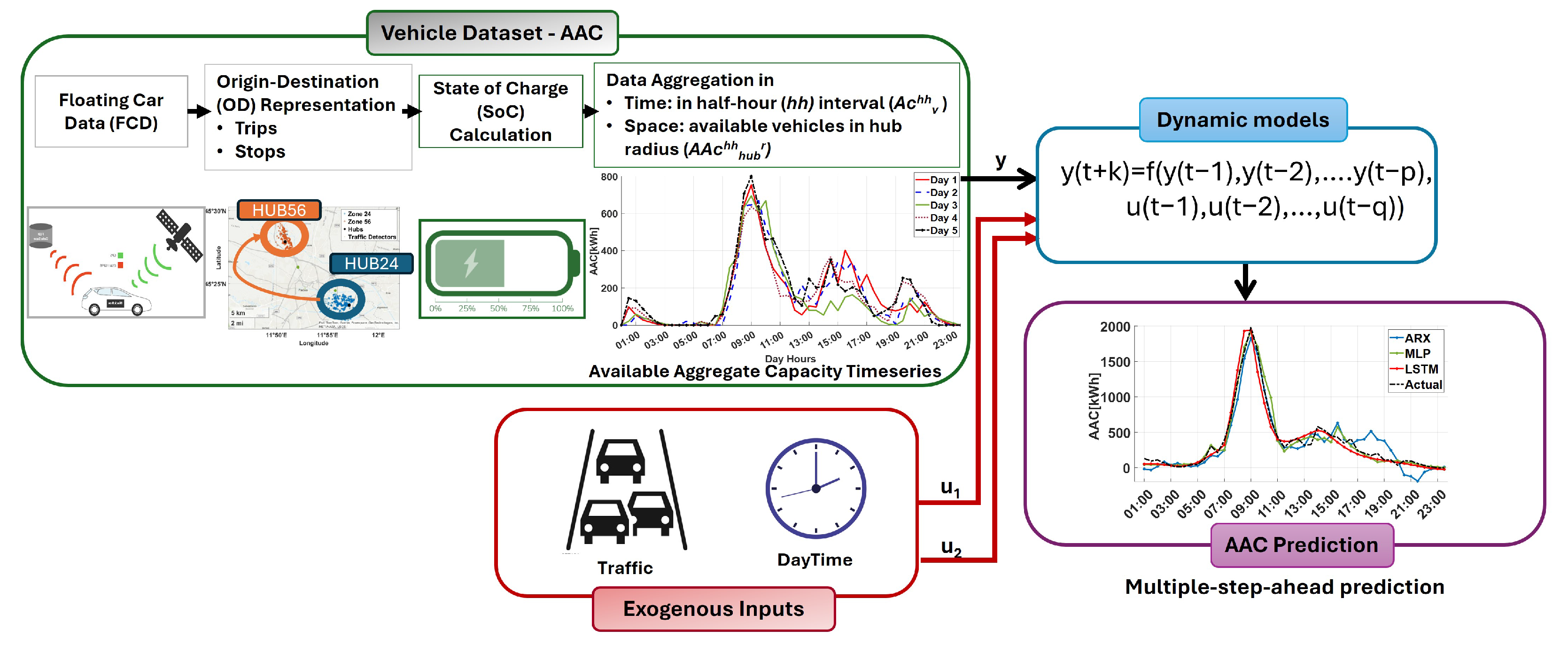
This section presents the framework proposed in this paper for estimating AAC within the required time horizon. Figure 1 shows a block diagram of the proposed procedure. The vehicle dataset block describes the acquisition of the floating car data, i.e., the real-time vehicle tracking data on status and localization, and its relevant features, such as origin–destination (OD), to extract the trips and stops to determine the state of charge ($SoC\%$) for each vehicle. A spatio-temporal analysis is then performed to calculate the AAC time series, i.e., the target variable for the prediction models. The areas of interest are selected by considering a distance radius, r, from the selected hub. This is the basis of the spatial aggregation, while the temporal aggregation was performed in half-hour ($hh$) intervals corresponding to the time scale of the intraday energy market, as indicated in the literature [25,26,31,32]. The exogenous inputs block is dedicated to the elaboration of the exogenous model inputs, i.e., the time of day and the traffic data collected at specific locations related to the analyzed hubs. The model block represents the dynamic models implemented with different identification approaches, which are discussed and compared below. Both linear and nonlinear models were implemented and compared with each other. The output of the model consists of the prediction of AAC over a given time window, adopting multiple-step-ahead prediction strategies. In the next subsections, the analyzed dataset and the used prediction models are discussed in detail.

2.1. Data Collection and Pre-Processing

The available vehicle dataset includes static data on vehicle categories and dynamic data including the geographical coordinates of vehicle routes. Basic vehicle information, including vehicle class, brand, registration year, type, fuel type and gross weight is included in the information form for each vehicle considered in the sample and used for virtual electrification of the vehicles. The vehicle identifier, date (the date on which the record was recorded), timestamp (the time at which the record was recorded), coordinates (the geographical location: longitude and latitude), instantaneous speed, road type (urban, extra-urban, highway) and directional angle are included in the daily trip logs, which contain all trips made by the sampled vehicle in chronological order. However, the dataset does not include information on the purpose of the registered trips (e.g., work or study) or the type of activity the vehicle was engaged in.

The datasets can be processed to obtain the AAC and other aggregated information in the space and time domain with a parametric T-hour ($Th$) time interval. The first step is to identify V2G points of interest (i.e., candidate hubs) as V2G services rely on the identification of suitable geographical zones based on vehicle data analysis. The movement from one location (origin) to another (destination) (OD) to perform one or more tasks is called a trip. Access to telemetry data enables the collection of trip information with FCD, which enables continuous vehicle tracking over time [42]. The vehicle position (a sequence of geographic coordinates) and status (traveling or stopping states) are also given. Two consecutive data points of a particular vehicle can be used to identify the start and end of a trip and to detect major changes in vehicle position based on the corresponding status information. A journey or trip chain refers to a series of trips linked such that the destination of one trip coincides with the starting point of the next. Consequently, the activity stops are determined using the fine-grained FCD. For EVs, this approach enables the determination of battery levels and additional tasks performed after each stop. The proposed process is based on measurements of a vehicle’s speed and engine state. The process evaluates these measurements to determine whether the vehicle is traveling very slowly or has come to a complete stop. Observations, where the vehicle has stopped at a bottleneck but appears to be parked, are the main cause of inaccuracies in identifying stops from vehicle data. The method guarantees that only active stops (e.g., longer than a pre-defined threshold and far away from intermediate stops/service points such as gas stations) are classified as such in the result by evaluating both the speed during the previous time interval and the geographical coordinate data as well as the engine status.

The zoning process aligns with the study area data, identifying potential locations for V2G service implementation, such as parking lots near cinemas, retail centers, and workplaces.

Following the integration of dynamic mobility data with static vehicle category data, the entire dataset is processed to virtually electrify each vehicle entry. This virtual electrification process entails linking each car model in the dataset to an equivalent battery electric vehicle (BEV) and assigning an energy value, measured in kWh, to its battery pack.

The activity is performed by:

• a classification often used by manufacturers
• market research on the characteristics of battery packs used in EVs
• the assignment of an average energy value in relation to the class of the vehicle reported in the database

The classification aims to distinguish different car models and categorizes them based on technical specifications, as shown in

Table 2. Passenger car classification and average energy value for each segment.

Segment	ACEA Classification	Description	Average Energy Value [kWh]
A	Small	City cars	28
B	Small	Small cars	30
C	Lower Medium	Medium cars	70
D	Upper Medium	Large cars	74
E	Luxury	Executive cars	71
F	Luxury	Luxury cars	86
S	-	Sport coupes	101
J	SUV	Sport utility cars	74
M	MPV	Multi purpose cars	66

[45]. The market research led to the identification of 60 BEV models currently on the market in Italy. For each model, the energy of the installed battery pack was recorded and, if the vehicle supported more than one solution, the one with the highest energy was selected. The data were then processed by determining the number of vehicles in each specific segment and calculating the average battery energy value for that segment. For each segment, the energy consumption per kilometer traveled was also assigned. Each vehicle in the database was subsequently classified and virtually electrified by assigning an equivalent energy value to the battery pack (Table 2).

The next step involves mapping trips and stops by spatially aggregating data to create a subset for each candidate V2G hub. Additionally, time aggregation is performed with a parametric $Th$ interval, generating a time series that serves as the target for the dynamic prediction model. The calculation of the AAC time series for a specific V2G hub leverages the concept of the percentage state of charge ($SoC\%$), which can be determined as an indirect measure of both distance traveled and V2G stop intervals.

The minimum battery charge ($So{C}_{min}$) that each vehicle must maintain after transferring energy to the grid is taken into account when highlighting participation in V2G services. In particular, $SoC\%$ calculation can be performed under specific hypotheses [31]: $SoC=100\%$ at the beginning of each day; the minimum state of charge that must be maintained can be set as a fixed value. It is determined as the maximum between a selected value ($So{C}_{min}=30\%$) and the one obtained as the charge necessary to cover the remaining part of the travel chain. To calculate the $SoC\%$ at each step of the trip, other key parameters must be considered: the energy consumption per kilometer traveled, which varies depending on the vehicle segment, and the discharge rate during the V2G plug-in, which is fixed at 22 kW for simplification purposes. For simplification, conventional energy transfers from the power grid to the vehicle while it is connected to a V2G system are not considered. The available capacity of a vehicle ($A{C}_v$) is derived from the simulated $So{C}_v$, reflecting the $SoC\%$ for each individual vehicle. Specifically, $A{C}_v^{Th}$ denotes the capacity of each vehicle to supply energy to the grid within a time interval that has been fixed to a half-hour $T_{hh}$:

$$A{C}_v^{T_{hh}}=max(So{C}_v^{T_{hh}}-So{C}_{min},0)\times B{C}_v$$

(1)

where $B{C}_v$ denotes the vehicle’s battery capacity, assumed to correspond to the average energy value for its vehicle segment, as outlined in Table 2. Equation (1) identifies vehicles eligible for V2G activity: if $So{C}_v^{T_{hh}}$ does not exceed the predefined $So{C}_{min}$, then $A{C}_v^{T_{hh}}$ is zero, indicating that the vehicle cannot contribute energy to the grid.

The space aggregation is based on the assumption that the vehicles parked for a period exceeding an interval $T_{hh}$ in the selected area related to a specific hub and determined in the zoning procedure would participate in the V2G activities. In particular, a vehicle parked in this area at a given time interval, and respecting the $So{C}_{min}$ requirement, is considered available ($a{v}_{Hub}$) to provide energy into the V2G system in that time interval. The target feature to be predicted is the aggregated available capacity ($AA{C}_{Hub}^{T_{hh}}$) in a $T_{hh}$ interval in the hub zone ($Hub$). It is defined in the following equation:

$$AA{C}_{Hub}^{T_{hh}}=\sum _{a{v}_{Hub}}A{C}_v^{T_{hh}}$$

(2)

An additional dataset comprising traffic flow information, i.e., specifically vehicle counts, is integrated to capture traffic dynamics on motorways and main roads near the designated V2G hub zones. These data provides insights into traffic density and movement patterns, enhancing the analysis by reflecting real-time conditions in areas proximate to potential V2G hubs. The level of the vehicle flows as well as the expansion to the universe of investigation can exploit the information coming from the traffic counts, i.e., counts of users (vehicle) flows, on some elements (links–roads) of the transportation supply system (network). Such information can be easy to obtain, often automatically through sensors or cameras located in designed road sections. In particular, count locations should be designed with respect to their information content and their use, e.g., origin–destination demand estimation.

The above extraction and pre-processing structure are applied to extract the AAC and the traffic data on the different aggregation points for the whole observation period. Considering the large dataset needed by AI approaches, a data augmentation procedure has been finally applied, consisting of increasing the available data by adding uniform noise with a maximum amplitude of 10%, increasing the amount of available data tenfold.

2.2. Dynamical Models

In this paper, we compare the performance and the transferability of different classes of model implemented with state-of-the-art methodologies. Both linear and nonlinear data-driven models have been considered: ARX models, external dynamics nonlinear models implemented with MLPsand internal dynamics nonlinear models implemented with LSTM networks.

The ARX model is given by:

$$AAC\left(t\right)=\sum _{k=1}^n{a}_k·AAC(t-k)+\sum _{k=1}^m{b}_k·T(t-k)$$

(3)

where $AAC(t-k)$ for $k=1,\cdots ,n$ are the past samples of the output variable, T is the input vector, $a_k$ and $b_k$ are the model coefficients identified using the least square method through the experimental dataset and n (model order) and m (number of input regressors) have been determined using optimization criteria. The described model is designed to perform one-step-ahead prediction. The prediction over a longer time horizon is obtained by iterating Equation (3), using estimated values of the output.

In the nonlinear ARX model implemented through MLPs, the following relation is considered:

$$AAC\left(t\right)=f\left(AAC\right(t-1),AAC(t-2),\cdots ,AAC(t-n),T(t-1),T(t-2),\cdots ,T(t-m\left)\right)$$

(4)

where f is a nonlinear function implemented by the MLP through multiple hidden layers constituted by neurons with a nonlinear activation function. The n and m parameters were selected to be equal to the ones identified for the ARX model. The hyperparameters to be optimized are the number of fully connected layers, the layer size and the activation function.

An LSTM network belongs to the recurrent neural network class that processes input data by iterating over time steps and updating the internal state that retains information from the previous time steps. A sequence-to-sequence LSTM neural network can predict future values in a time series or sequence based on the preceding time steps as input [46]. An LSTM architecture consists of a sequence input layer, with size depending on the number of input data features, LSTM hidden layers with ReLU activation and dropout implementation to avoid overfitting, a fully connected layer and a regression layer. The hyperparameters to be optimized are the number of LSTM layers and units and the dropout probability.

The different models were compared in terms of key performance indicators, such as the root mean squared error (RMSE) and the coefficient of determination ($R^2$) [47].

Let $X_i$ and $Y_i$ represent the predicted and actual values for the i-th data point, respectively, $\overline{Y}$ denote the mean of the actual values and m the number of data points. The RMSE is defined as:

$$\mathrm{RMSE}=\sqrt{{\displaystyle \frac{1}{m}}\sum _{i=1}^m{(X_i-Y_i)}^2}$$

(5)

Its units of measurement correspond to those of the predicted variable. The optimal value for RMSE is 0, while its maximum value extends to $+\infty$.

The $R^2$ coefficient is defined as follows:

$$R^2=1-{\displaystyle \frac{{\sum }_{i=1}^m{(X_i-Y_i)}^2}{{\sum }_{i=1}^m{(\overline{Y}-Y_i)}^2}}$$

(6)

It can be interpreted as the proportion of the variance in the dependent variable that is predictable from the independent variables. The $R^2$ is adimensional; its optimal value is 1, while its minimum value extends to $-\infty$.

2.3. The Veneto Case Study

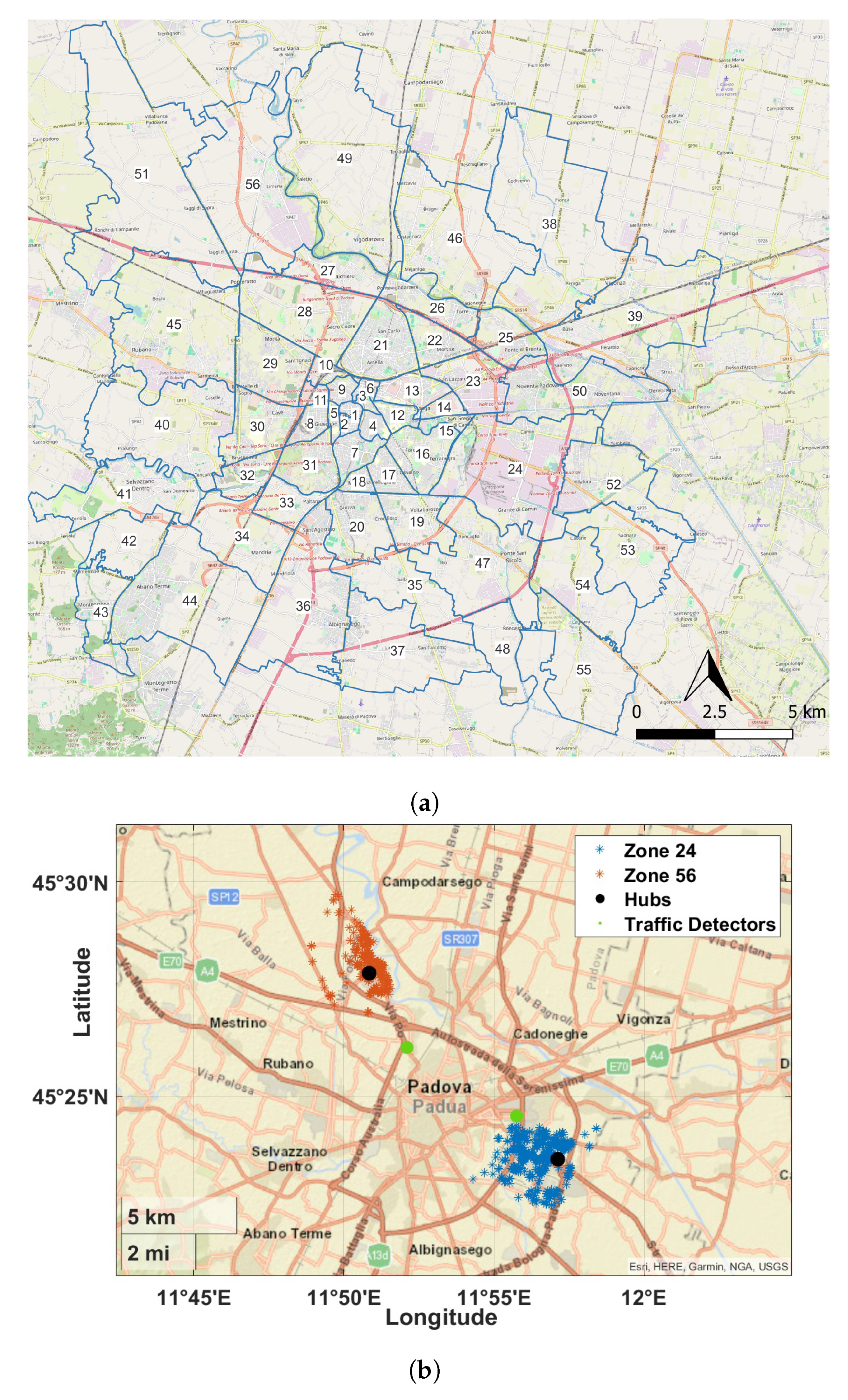
The methodology for estimating the potential energy that can be fed into the electrical grid was applied to Padua, a city in the Veneto region (northern Italy), the third largest region in Italy where EVs are registered. The city of Padua and thirteen smaller neighboring municipalities form the study area. The total population is around 370,000 inhabitants, mainly concentrated in the center of Padua, where the residential density is over 58 inhabitants per hectare. Furthermore, the study area has a total of less than 7000 stores with about 24,000 retail employees, mainly located in the historic city center and in the small town of Abano Terme. There are about 5000 warehouses with about 18,000 employees, mainly located west of the city center, close to the border with Noventa Padovana, where a large warehouse center is located. Finally, the study area was divided into 56 different zones (Figure 2a), taking into account the characteristics of land use (e.g., inhabitants, employees, stores) and emphasizing the homogeneity of functions (e.g., residential area, shopping area, industrial area). Based on the identified zones and the driving patterns resulting from the analysis of the studied vehicles (i.e., using FCD), some points of interest for the location of the stations for V2G services could be identified. Forty-five possible points of interest were identified, including shopping malls, hospitals, train stations, universities, large parking lots in high traffic areas (e.g., city centre), cinemas, stadiums and some supermarkets. It was also checked whether these were areas of high attraction by comparing them with the aggregated points related to the destinations of the trips recorded in the study area on the days studied. Of these 45 points, 2 more relevant locations were selected to which the final energy assessment study was applied. These are a peripheral area with medium traffic volume and medium stops (i.e., zone 56) and an area with high traffic volume and medium-short stops (i.e., zone 24).

The available dataset consists of observations collected over five working days during the autumn period (October–November 2018) on selected weekdays:

• Day1: Monday 15 October 2018
• Day2: Monday 22 October 2018
• Day3: Wednesday 7 November 2018
• Day4: Thursday 15 November 2018
• Day5: Friday 23 November 2018

The selected working days were analyzed for variability in meteorological conditions, and no significant differences were found, as all days had favorable weather according to historical databases. Consequently, no further investigation into the impact of weather, weekends or holidays [26,34] on the predictive models was conducted. The case study has been developed for testing the proposed methodology in terms of both using easy-to-obtain data that well describe the traffic conditions and outcomes provided. The used data refer to 2018, given that a large dataset was available covering 5 full working days of a large sample of vehicle that, during the days of survey, drove in one of the roads of the study area. For such days of the survey, several traffic counts within and outside the study area were available. These data allowed validation of the flows estimated. Furthermore, the goodness and robustness of these data was the objective of further studies, which highlighted the robustness of the traffic forecast. See, for example, [42]. Therefore, to use such data allowed us to really test our proposed methodology by applying it to a well representative case study. After a comprehensive data-cleaning process, which involved discarding records with incomplete entries, the dataset was analyzed to investigate trip patterns and durations. In total, 29,158 vehicles were examined, resulting in approximately 70,000 recorded trip chains over the course of the five-day observation period.

In the land-use analysis, zoning is performed using data from the study area to identify optimal locations for implementing V2G services. Figure 2b provides an initial analysis of mobility data from the Veneto region, illustrating the distribution of vehicle stops within the study area for a sample day. This visualization enables the identification of zones and potential hubs suitable for V2G services. Figure 2b shows the location of two traffic detectors monitoring traffic flow toward the identified zones, further supporting hub placement decisions. The vehicles parked refer mainly to systematic travels and the methodology refers to a planning horizon as well as to not only specific parking lots but also to parking zones. Then, according to specific traffic situations, the users could not reach the specific locations but the area should remain the same given that it is assumed that traffic jams can cause drivers to change their path but not their destination or mode of travel.

A large sample of automated traffic counts was available in the Veneto region, comprising traffic counts on several motorways and main roads. This dataset enabled the characterization of traffic flows in terms of vehicle counts over five days corresponding to the mobility data sample days. To reconstruct the road network flows and to identify the sampling rate in the study area, it was necessary to acquire information relating to traffic counts on the ANAS and motorway networks (CAV operators, Autovie Venete, Autostrade per l’Italia). Furthermore, in five road sections among those of the ANAS network, manual counts were also carried out, confirming the reliability of the data from the automatic ANAS surveys. From the analysis of the hourly data on the ANAS network, classified by vehicle type, the average hourly profiles for cars and commercial vehicles were identified. It has been revealed that, on average, in all the surveyed sections, the hourly profiles are similar, showing two peak time slots (a morning one between 6:00 and 8:00 and an afternoon one between 16:00 and 18:00). Between 8:00 and 16:00, the flow of cars remains almost constant, settling between 4% and 7% of the total daily value measured in correspondence with the surveyed section. A given similarity between the hourly distribution of cars and light commercial vehicles (less than 3.5 t p.t.t.) has been identified. From the analysis of the temporal profile of the equivalent flow, it was possible to identify the 7:00–8:00 time slot as the morning peak, with an average equivalent flow of 1252 vehicles/hour (i.e., 7.2% of the average daily flow passing through the relevant sections) and the 17:00–18:00 time slot as the afternoon peak, with an equivalent flow of 1301 vehicles/hour (i.e., 7.5% of the average daily traffic in the relevant sections).

3. Results and Discussion

In this section, the results for the one-step- and the three-step-ahead prediction of AAC are presented. The linear ARX model, the nonlinear external dynamic neural model implemented with MLPs and the nonlinear internal dynamic model implemented with LSTM are compared. In the first step, a preliminary analysis was performed to select the relevant model inputs.

For this purpose, four different configurations of model inputs were compared:

• Model A: pure autoregressive model;
• Model B: autoregressive model with the daytime (D) as exogenous input;
• Model C: autoregressive model with traffic (Tr) as exogenous input;
• Model D: autoregressive model with D and Tr as exogenous inputs.

Akaike’s information criterion (AIC) was used to select the optimal model order and finite delay in a grid search procedure.

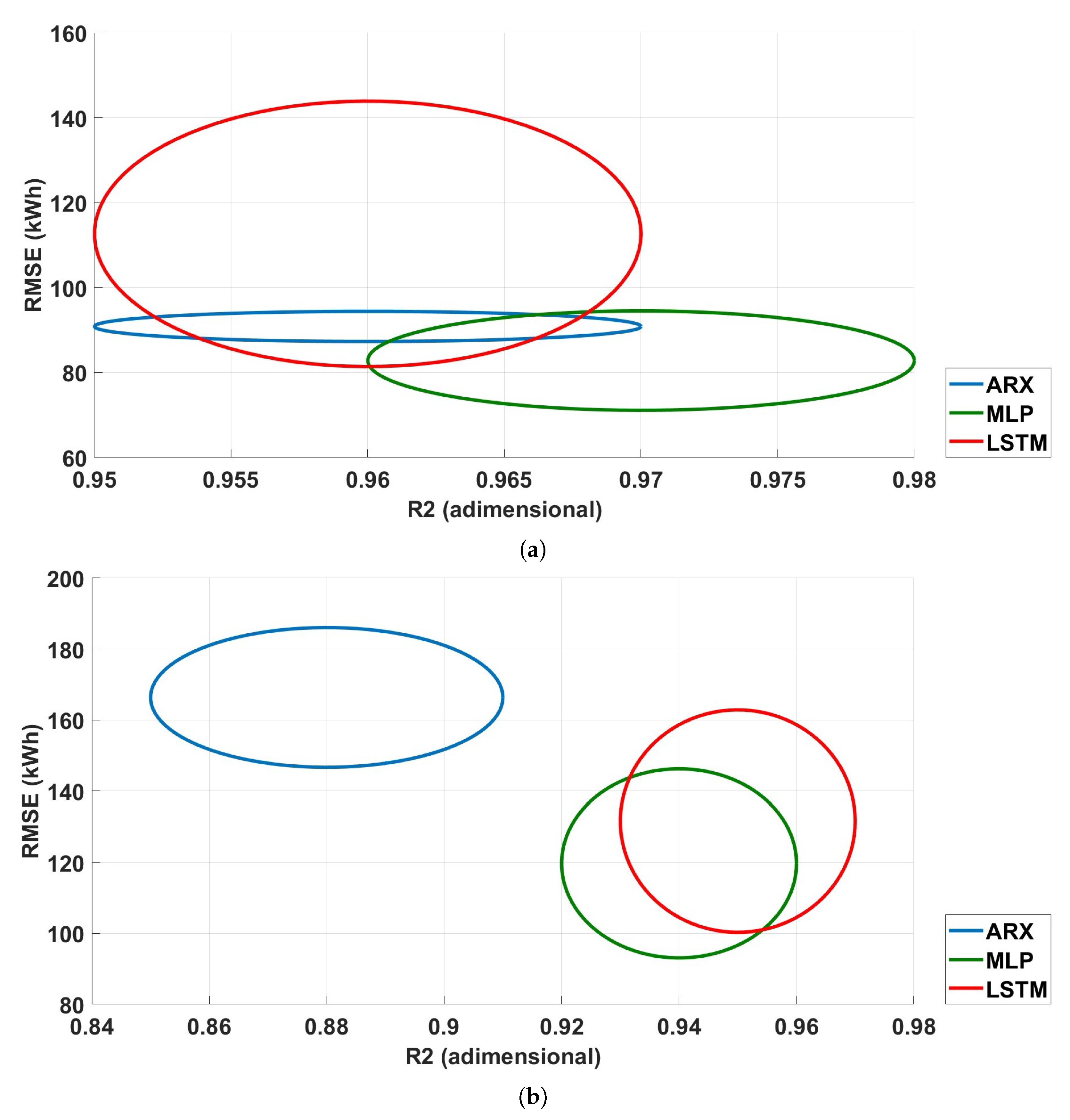
Due to the data scarcity besides the data augmentation procedure mentioned in Section 2, to improve the statistical significance of the reported analysis, a k-fold cross-validation procedure was considered. In particular, the five days of data available were split into four (training and validation) and one (testing) following a 5-fold cross-validation method. The results obtained are shown in Figure 3, where the four input configurations are compared when the one-step- and three-step-ahead predictions are considered. The figure refers to the ARX models trained and tested on Hub 24. Each ellipse shows the distribution of the performance indices used for the test dataset: the RMSE and the $R^2$.

The center of each ellipse corresponds to the mean value over the 5-fold cross-validation, while the dimensions of the axes correspond to the obtained standard deviation.

It can be seen from the figure that the best performance is achieved when traffic is included as an input variable (Model C), while adding the daytime to the input vector is not relevant. Specifically, for the one-step-ahead prediction (Figure 3a), the $R^2$ index improves from about 0.92 to 0.94 and the RMSE decreases from 127 to 90. An even more significant improvement results for the three-step-ahead prediction (Figure 3b); in this case, from Model A to Model C, the $R^2$ increases from 0.43 to 0.88, while the RMSE decreases from 373 to 163.

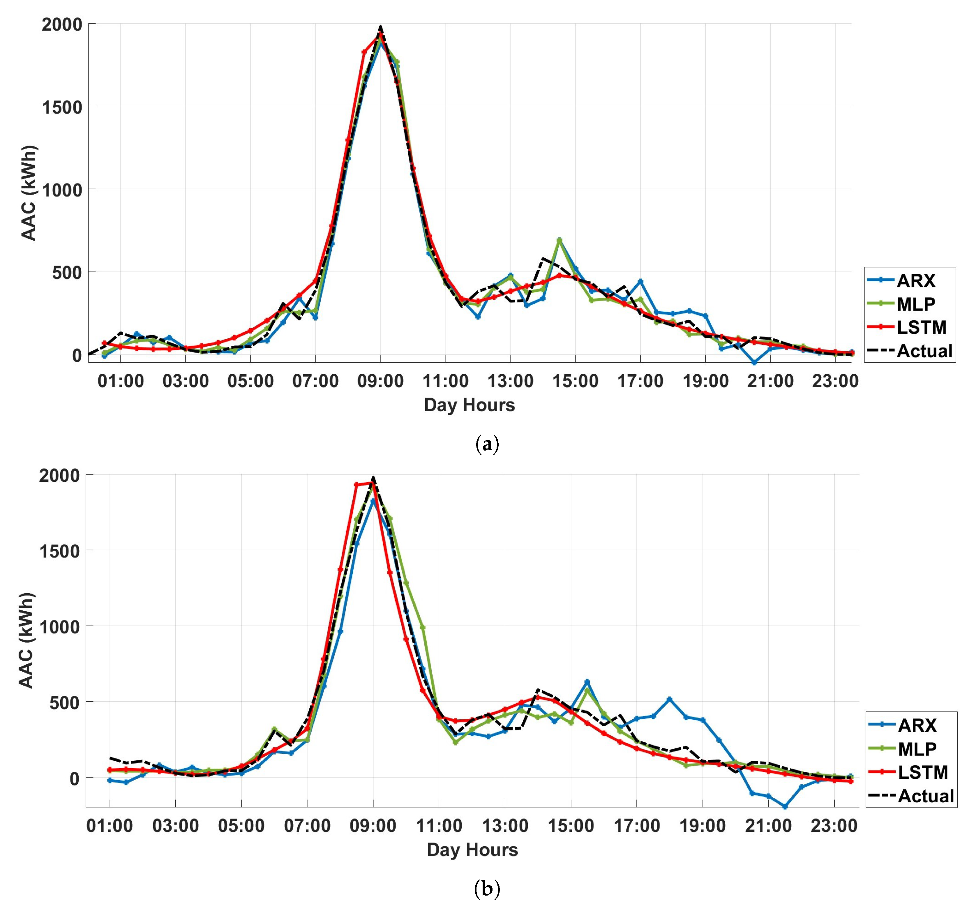
The time evolution of the output variable for the ARX models is shown in Figure 4 for both the one-step- and the three-step-ahead prediction. It can be observed that models that include traffic as an input maintain their performance when a three-step-ahead prediction is calculated. This does not apply to models that contain only past output values.

Table 3. Performance analysis of the different ARX models for Hub 24. The mean and standard deviations obtained during the 5-fold procedure are reported for the training and test data.

	One-Step-Ahead Prediction				Three-Step-Ahead Prediction
	Training		Test		Test
	RMSE	${\mathit{R}}^{\mathbf{2}}$	RMSE	${\mathit{R}}^{\mathbf{2}}$	RMSE	${\mathit{R}}^{\mathbf{2}}$
no input	126.48 ± 9.63	0.92 ± 0.02	127.61 ± 10.12	0.92 ± 0.02	373.90 ± 40.51	0.43 ± 0.06
daytime	125.52 ± 9.50	0.92 ± 0.02	126.59 ± 9.94	0.92 ± 0.02	366.22 ± 38.79	0.41 ± 0.07
traffic	112.53 ± 10.71	0.94 ± 0.02	90.85 ± 3.55	0.96 ± 0.01	166.38 ± 19.68	0.88 ± 0.03
traffic & daytime	113.11 ± 10.57	0.93 ± 0.001	90.92 ± 3.58	0.96 ± 0.01	166.5 ± 20.0	0.88 ± 0.03

shows the performance of the best model for each input configuration. A statistical analysis was performed on the five different folds considered for Hub 24.

The same comparison was also carried out with nonlinear models. In the case of both MLP and LSTM, the optimal choice of parameters involves traffic among the inputs. The same regressor structure used for the ARX model was also considered for the MLP model. The MLP hyperparameters consist of the number of hidden layers, the neurons per layer and the activation function. A grid search optimization procedure was applied, resulting in the following configuration: three hidden layers with ten neurons each using the ReLU activation function. Optimization of the hyperparameters of the LSTM network resulted in a structure consisting of three layers with five neurons each.

From

Table 4. Performance analysis of the linear and nonlinear models, including the traffic as input, for Hub 24. The mean and standard deviation obtained during the k-fold procedure are reported for the training and test data in the case of both one-step- and three-step-ahead prediction.

	One-Step-Ahead Prediction				Three-Step-Ahead Prediction
	Training		Test		Test
	RMSE	${\mathit{R}}^{\mathbf{2}}$	RMSE	${\mathit{R}}^{\mathbf{2}}$	RMSE	${\mathit{R}}^{\mathbf{2}}$
ARX	112.53 ± 10.71	0.94 ± 0.02	90.85 ± 3.55	0.96 ± 0.01	166.38 ± 19.68	0.88 ± 0.03
MLP	47.64 ± 4.15	0.99 ± 0.002	82.77 ± 11.74	0.97 ± 0.01	119.91 ± 26.62	0.94 ± 0.02
LSTM	79.62 ± 10.15	0.98 ± 0.01	112.64 ± 31.25	0.96 ± 0.01	131.58 ± 31.29	0.95 ± 0.02

and Figure 5, it can be seen that the MLP shows the best performance in terms of both RMSE and $R^2$ for one-step-ahead prediction. The ARX shows a lower variance in terms of RMSE compared to the other methods. The LSTM shows performance similar to the MLP. The results for the three-step-ahead prediction (Figure 5b) show a significant drop in performance for the ARX, while the nonlinear models work consistently and again show similar performance. Values of $R^2$ = 0.94 and $R^2$ = 0.95 are obtained for MLP and LSTM, respectively, while $R^2$ = 0.88 is achieved for the ARX model.

Time evolution comparison over one day, which is part of the test set, for the linear and nonlinear models under analysis is reported in Figure 6, where both one-step- and three-step-ahead predictions are shown. The results confirm the superiority of the MLP model, although the other models also provide suitable results, especially in correspondence to the AAC peak.

Similar results were obtained for Hub 56, as summarized in

Table 5. Performance analysis of the linear and nonlinear models, including the traffic as input, for Hub 56.

	One-Step-Ahead Prediction				Three-Step-Ahead Prediction
	Training		Test		Test
	RMSE	${\mathit{R}}^{\mathbf{2}}$	RMSE	${\mathit{R}}^{\mathbf{2}}$	RMSE	${\mathit{R}}^{\mathbf{2}}$
ARX	64.08 ± 7.30	0.88 ± 0.02	61.46 ± 9.74	0.89 ± 0.02	98.58 ± 11.89	0.72 ± 0.04
MLP	40.45 ± 6.36	0.95 ± 0.01	55.04 ± 6.77	0.91 ± 0.02	69.58 ± 9.90	0.87 ± 0.04
LSTM	42.58 ± 4.3	0.95 ± 0.01	70.37 ± 16.62	0.88 ± 0.04	73.77 ± 15.08	0.87 ± 0.04

, for the best-performing model that has traffic as input.

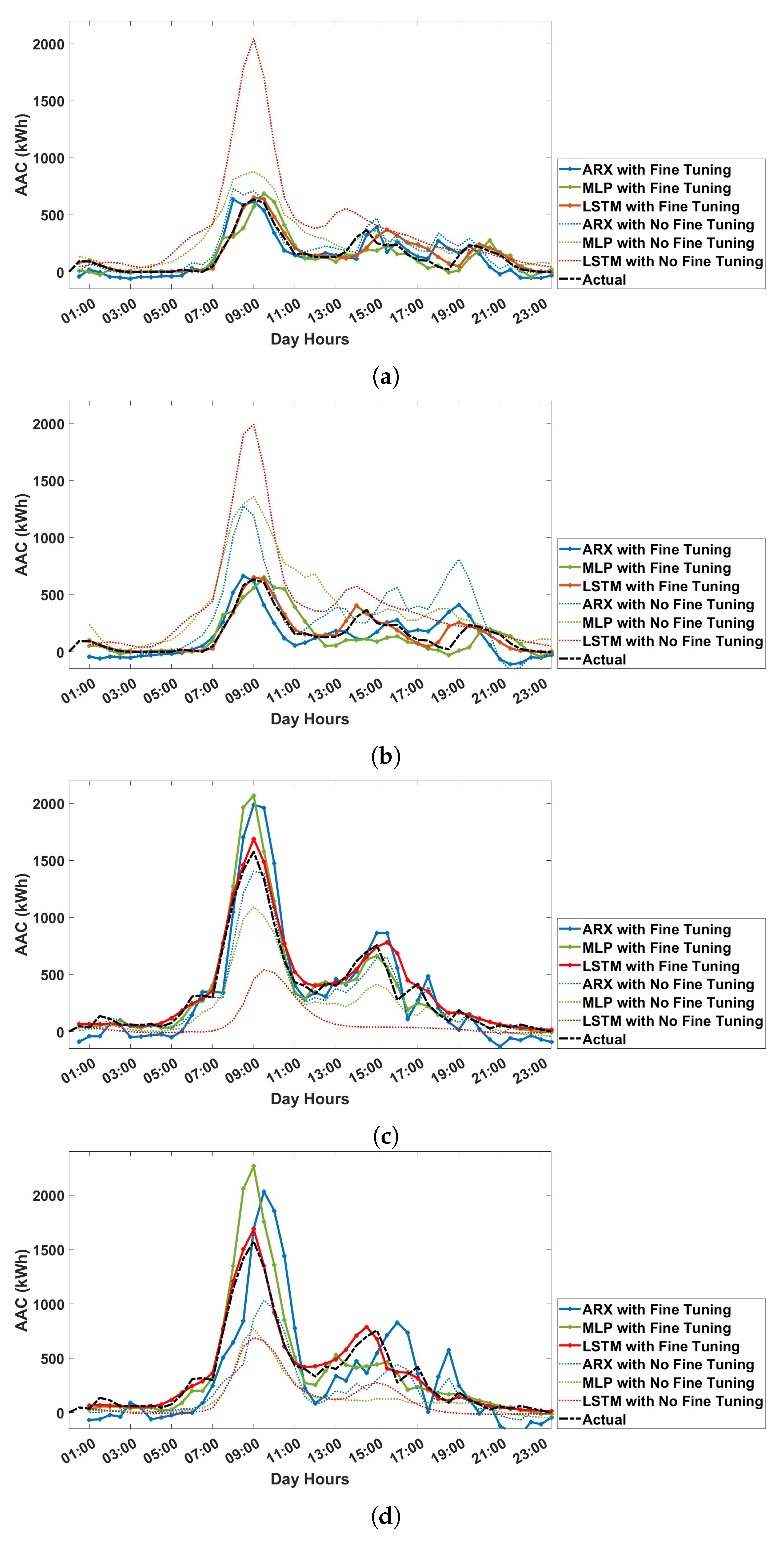
Model Transferability Analysis

In this section, the transferability of the models obtained from one hub to another is analyzed. Two different scenarios are considered. In the first scenario, it is assumed that no data are available for the target domain. This means that the models derived for the source zone are simulated directly with the inputs of the target zone to calculate the predictions. In the second scenario, it is assumed that only a limited amount of data are available from the target area. In this case, the model trained based on the source data is fine-tuned using only one day of data collected in the target area (20% of available data). In the case of MLP and LSTM, this means a few training epochs with the new dataset. In the case of the ARX model, a scaling of the target domain dataset is performed to match it to the source domain dataset. The models obtained from Hub 24 were simulated with the input data from Hub 56 and, vice versa, to implement the first scenario. The results are shown in

Table 6. Performance analysis for the transfer of the model derived for Hub 24 to Hub 56, and vice versa.

		One-Step-Ahead Prediction				Three-Step-Ahead Prediction
		RMSE	${\mathit{R}}^{\mathbf{2}}$	$∆$RMSE	$∆$${\mathit{R}}^{\mathbf{2}}$	RMSE	${\mathit{R}}^{\mathbf{2}}$	$∆$RMSE	$∆$${\mathit{R}}^{\mathbf{2}}$
Transfer Hub 24 ->Hub 56	ARX	118.63 ± 9.38	0.67 ± 0.06	−48%	−25%	299.43 ± 20.94	0.04 ± 0.80	−67%	−94%
	MLP	159.25 ± 20.82	0.52 ± 0.07	−66%	−43%	317.02 ± 28.78	0.20 ± 0.09	−78%	−77%
	LSTM	362.25 ± 34.51	<0	−81%	<−100%	385.39 ± 26.198	<0	−81%	<−100%
Transfer Hub 56 ->Hub 24	ARX	140.84 ± 12.17	0.87 ± 0.07	−35%	−9%	327.70 ± 30.02	0.55 ± 0.13	−49%	−38%
	MLP	238.87 ± 38.61	0.22 ± 0.64	−65%	−77%	419.03 ± 69.70	<0	−71%	<−100%
	LSTM	423.87 ± 51.51	0.20 ± 0.15	−75%	−79%	384.95 ± 51.59	0.35 ± 0.03	−66%	−63%

.

The performance of the models obtained for Hub 24 and transferred to Hub 56 is not satisfactory. For example, the $R^2$ value of the ARX model decreases from 0.88 (see Table 5) to 0.67 for one-step-ahead prediction and from 0.72 (see Table 4) to 0.04 for three-step-ahead prediction, making the model unsuitable. Better results were obtained by transferring the model from Hub 56 to Hub 24. In this case, the ARX model decreased from 0.94 to 0.87 for the one-step-ahead prediction and from 0.88 to 0.55 for the three-step-ahead prediction. The performance degradation indices $∆$RMSE and $∆$$R^2$ are also included in the table. It should be noted that, in some cases, the $R^2$ is negative, so in these cases the chosen model fits worse than using the mean value as an estimator. Similar results are obtained for the other models. It can be concluded that none of the models achieves an adequate level of performance using the direct transfer method considered in the first scenario. The performance drop can be related to some differences in cluster characteristics. The hubs analyzed are a peripheral area with medium traffic volume and medium stops (zone 56) and an area with high traffic volume and medium-short stops (zone 24). The different characteristics of the two hubs are the main cause of the drop in performance when the models are transferred directly from one hub to the other. This is overcome by using a fine-tuning strategy.

The results obtained for the second scenario are shown in

Table 7. Performance analysis for the transfer with finetuning of the model derived for Hub 24 to Hub 56, and vice versa.

		One-Step-Ahead Prediction				Three-Step-Ahead Prediction
		RMSE	${\mathit{R}}^{\mathbf{2}}$	$∆$RMSE	$∆{\mathit{R}}^{\mathbf{2}}$	RMSE	${\mathit{R}}^{\mathbf{2}}$	$∆$RMSE	$∆$${\mathit{R}}^{\mathbf{2}}$
Transfer Hub 24 ->Hub 56	ARX	99.90 ± 7.11	0.69 ± 0.03	−38%	−22%	139.92 ± 14.26	0.41 ± 0.09	−30%	−43%
	MLP	81.22 ± 11.59	0.80 ± 0.03	−32%	−12%	105.13 ± 13.70	0.68 ± 0.06	−34%	−22%
	LSTM	80.98 ± 11.81	0.81 ± 0.07	−14%	−8%	83.85 ± 8.90	0.80 ± 0.06	−13%	−8%
Transfer Hub 56 ->Hub 24	ARX	156.43 ± 25.15	0.87 ± 0.07	−42%	−9%	239.26 ± 33.72	0.58 ± 0.13	−43%	−34%
	MLP	116.33 ± 14.11	0.93 ± 0.02	−29%	−4%	148.95 ± 37.86	0.88 ± 0.07	−19%	−6%
	LSTM	148.31 ± 35.54	0.89 ± 0.09	−28%	−7%	148.03 ± 45.23	0.89 ± 0.09	−12%	−6%

. In this case, the ARX shows better performance with respect to the first scenario, when both the one-step-ahead and three-step-ahead predictions are considered ($R^2$ = 0.69 and $R^2$ = 0.41, respectively). However, the results are still not satisfactory. The nonlinear methods show, instead, quite good performance. Specifically, in the case of transfer from Hub 24 to Hub 56, the MLP decreases from $R^2$ = 0.95 (see Table 5) to $R^2$ = 0.80 for the one-step-ahead prediction and from $R^2$ = 0.95 (see Table 4) to $R^2$ = 0.68 for the three-step-ahead prediction. The LSTM decreases from $R^2$ = 0.87 (see Table 5) to $R^2$ = 0.81 for the one-step-ahead prediction and from $R^2$ = 0.87 (see Table 4) to $R^2$ = 0.80 for the three-step-ahead prediction, revealing this to be the best method as regards transferability. Even better results are obtained for the transfer from Hub 56 to Hub 24. The global analysis of the model performance leads to the conclusion that the LSTM performs better than the other approaches considered, as also shown by the time evolutions reported in Figure 7.

Although the proposed analysis was only tested on two hubs, in the absence of further experimental data the transfer learning approach is a promising method for handling the prediction of AAC in new hubs, reducing the need for data collection. In the presence of multiple hubs, the ability to cluster the hubs, based on their characteristics, can further improve the transfer procedure.

4. Conclusions

This study presents an analysis of linear and nonlinear models to estimate the AAC of electric vehicles for V2G applications based on FCD. A case study in Padua, Italy, is used to demonstrate the potential for AAC estimation by analyzing mobility patterns and traffic data. The results suggest that FCD, complemented by telematics and location-based applications, provides an effective basis for identifying private car trips that could contribute to V2G services. Furthermore, the use of both linear and nonlinear dynamic models enables the prediction of AAC at one- and multiple-steps ahead, providing valuable insights into the predictive capabilities of different input variables.

Specifically, linear dynamic ARX models, incorporating traffic data as exogenous inputs, showed good performance for both one-step- and multi-step-ahead prediction and are intrinsically interpretable and easy to use. However, nonlinear models, in the form of nonlinear ARX, implemented by MLP and LSTM structures, showed better performance at the two hubs considered, at the cost of losing interpretability.

Moreover, the analysis of the transferability of the predictive models from one aggregation point to another underlines the applicability of this approach in different urban areas to overcome the challenges of data scarcity. Two different scenarios of model transfer were analyzed. The direct transfer of the trained models from one hub to another showed poor performance for all models considered. The second scenario, which consists of fine-tuning the source model considering only a small amount of data from the target area, led to good results, especially for the LSTM-based architecture. This study thus contributes to research by providing a scalable and transferable method for predicting AAC, which ultimately supports the advancement of V2G technologies and grid resilience. The availability of data belonging to multiple hubs will make it possible to implement different approaches to improve model transfer performance by incorporating additional contextual features, such as indicators of land use types, and temporal variations (e.g., peak and off-peak hours), to better capture the unique characteristics of each hub. In addition, potential future approaches will involve clustering aggregation points based on common characteristics before model training to ensure a better fit of models to the target area. It is expected that these measures will improve the robustness of the model and its applicability in different urban contexts. Further developments will include the following: considering the stochastic nature of the state of charge when approaching parking locations (e.g., variations in routes taken) as well as when departing to carry out subsequent daily activities; investigating additional variables, such as weather conditions, calendar days and public holidays, which could potentially influence AAC. In this context, an interpretability analysis could be conducted to evaluate the significance of each predictor.