Stochastic Approaches to Energy Markets: From Stochastic Differential Equations to Mean Field Games and Neural Network Modeling

Abstract

This review paper examines the current landscape of electricity market modelling, specifically focusing on stochastic approaches, transitioning from Mean Field Games (MFGs) to Neural Network (NN) modelling. The central objective is to scrutinize and synthesize evolving modelling strategies within power systems, facilitating technological advancements in the contemporary electricity market. This paper emphasizes the assessment of model efficacy, particularly in the context of MFG and NN applications. Our findings shed light on the diversity of models, offering practical insights into their strengths and limitations, thereby providing a valuable resource for researchers, policy makers, and industry practitioners. The review guides navigating and leveraging the latest stochastic modelling techniques for enhanced decision making and improved market operations.

1. Introduction

The liberalization of energy markets and the promotion of sustainable energy have introduced market uncertainties, affecting stakeholders’ decision-making processes. In the energy market, stochastic models are a specific class of mathematical approaches mainly used to take into account the challenges caused by managing uncertainties naturally arising when one aims to represent energy-characterizing variables and their dynamics correctly. Unlike deterministic models, where all input parameters are assumed to be known, stochastic models incorporate uncertainty in at least one input parameter, thus providing a more realistic framework for simulating the evolution of energy production and consumption and for describing the economic behaviours of energy-related assets.

Over the years, and increasingly in recent times because of both political and climatic factors, the need to accurately predict the aforementioned dynamics has become even more pressing. This need has led scientists belonging to a heterogeneous class of disciplines, from physics to mathematics, from climatology to artificial intelligence, to the development of increasingly sophisticated and precise models. Among them, solutions based on advanced tools specific to stochastic analysis in general and the theory of Stochastic Differential Equations (SDEs), in particular, have stood out. It is worth remembering that such models are typically characterized by not having explicit solutions. This lack has made it necessary to use considerable hardware resources, typically via the wise use of parallelization techniques, with specific reference to Graphical Processing Unit (GPU) structures interacting in real-time. In order to optimize computation flows, while at the same time containing execution times in the face of specific cost constraints, the development of hybrid SDE-based and Machine Learning (ML)-based schemes has been undertaken, with specific reference to the implementation of increasingly sophisticated neural networks (NNs).

In the present paper, we address the task of reviewing those stochastic methods that have shown their effectiveness in dealing with the dynamic analysis and forecasting of energy markets. In particular, we provide a comprehensive review of current trends in electricity market modelling, traversing from SDE to NN modelling, passing through Mean Field Games (MFGs). Indeed, as the demand for cleaner and more efficient energy solutions intensifies, understanding and adapting to the intricate dynamics of the market become increasingly crucial. By evaluating the strengths and limitations of existing models, this review aims to contribute to the ongoing discourse surrounding electricity market modelling, offering a roadmap for researchers, policy makers, and industry professionals keen on harnessing the potential of stochastic approaches.

Existing energy systems boast impressive strengths, being characterized by their ability to deliver reliable and consistent power to meet the demands of a growing global population. Centralized power generation has enabled economies of scale, efficient resource utilization, and stable energy supply. However, this centralized paradigm has limitations, especially as the world grapples with the urgent need for sustainable and resilient energy solutions. One notable limitation concerns the vulnerability of centralized power grids to natural disasters, cyber attacks, and other unforeseen events. Moreover, reliance on conventional fossil fuels has led to environmental concerns, prompting a paradigm shift towards renewable energy sources. The intermittent nature of renewable resources, such as solar and wind, adds a layer of complexity to the existing system. As we transition towards a more sustainable energy landscape, challenges in ensuring reliability, flexibility, and efficiency become apparent.

The generation, transmission, and distribution triad represents the core elements of energy markets. The landscape of power generation includes traditional sources like coal and natural gas alongside an increasing reliance on renewable sources such as solar, wind, and hydropower. Modelling the stochastic nature of renewable energy generation is a formidable task, considering the variability and intermittency associated with these sources. The transmission of electricity across vast networks involves intricacies related to load balancing, congestion management, and the integration of diverse energy sources. At the distribution level, these dynamics affect the delivery of electricity to end-users.

In exploring the energy landscape, we traverse the spectrum of SDEs while focusing on stochastic partial differential equations (SPDEs) to model standard financial instruments in energy markets. The strategy of market participants can be encapsulated through various mathematical models that leverage principles from economics, game theory, and optimization. To encompass the strategic interactions among market players, recognizing that energy markets are shaped not only by random fluctuations but also by the rational decision making of numerous participants, we focus on game theory models such as MFGs. MFGs capture the strategic interactions among rational agents seeking to optimize their objectives. This could involve generators determining bidding strategies, retailers optimizing procurement, and consumers adjusting their consumption patterns in electricity markets. MFGs are one of the most widespread models used to establish the Nash equilibrium. They are particularly relevant when modelling scenarios with many interchangeable market participants, such as consumers or small-scale generators, where individual actions collectively influence the market.

Another possibility relies on ML models, such as Reinforcement Learning (RL), which are RL techniques or use predictive analytics based on neural networks for forecasting market trends, electricity prices, and demand patterns. We harness the capabilities of NNs and sophisticated tools designed for pattern recognition and prediction. By leveraging the computational prowess of NNs, we aim to uncover hidden patterns, correlations, and trends within vast and intricate datasets. NNs become invaluable allies in forecasting energy trends, enhancing our ability to make informed decisions and predictions in an ever-evolving energy ecosystem.

Other models are based on optimization algorithms such as Linear Programming (LP) and Mixed-Integer Linear Programming (MILP), which are used to model the bid generation process, considering production costs, demand, and capacity limits as problem constraints.

The paper is organized as follows: Section 2 shows our motivation and paper identification methodology; an overview of the energy modelling market applications and methods is presented in Section 3. In Section 4, we review more recent SDE-based methods to model energy features; in Section 5, we focus on the most recent SPDEs method for financial contracts. In Section 6, we introduce the MFG paradigm with a plethora of applications in the energy sector; in Section 7, we present some key applications of ML and optimization algorithms in the energy sector. We conclude the article with Section 8, outlining future directions.

2. Review Scope and Motivation

Our aim is to review the presence and application of SDEs in energy market analysis while exploring their intersection with ML and neural networks (NNs), given their increasingly central role in this domain. In particular, we encompass a wide array of applications and prominent methodologies discussed in the literature, as shown in Figure 1. While many reviews exist, our goal is to provide a comprehensive one covering a wider perspective of energy modelling applications and approaches, providing the main concepts and theory behind them, and filling gaps left by previous analogous works. For example, in [1,2], the authors primarily focus on stochastic model classifications, while other works focus on specific applications or approaches [3,4,5] without providing a complete analysis, or they adopt a bibliometric perspective (see, e.g., [6]). Additionally, we explore emerging advancements, particularly in the context of AI-driven solutions, also discussing current trends and future directions within this rapidly evolving field.

As previously mentioned, our primary focus is to provide a broader perspective on the literature rather than merely citing a number of publications. Accordingly, we identify key papers across three main energy areas: SDEs, MFGs, and ML for energy. We also detail surveys covering these domains. For this review, we selected papers indexed in Scopus based on two main criteria: high impact (measured by citation count) and/or recent publication date.

3. Energy Modelling: Applications and Methods

Energy market modelling refers to the development and application of mathematical, computational, and statistical methods used to represent and analyze the dynamics of energy markets [7]. It involves simulating interactions between key participants, such as electricity generators, consumers, regulatory bodies, etc., to forecast market outcomes like prices, demand, and system reliability. Energy market modelling involves applying techniques such as agent-based modelling, mathematical and econometric analysis, ML models, and optimization to support decision making in policy development, strategic planning, and investment in energy systems. This modelling process helps to assess the impact of various economic, technical, and regulatory factors on market stability, pricing, investment requirements, and overall efficiency [8].

Figure 1 provides an overview of energy market applications and modelling methods, while

Table 1. Overview of applications and approaches.

Application Area	Techniques	Examples
Electricity prices and production modelling	Mean-Reverting Processes, Jump-Diffusion Models, Fractional Brownian Motion, Regime-Switching Models, Reinforcement Learning, Hybrid Models, ML, DNN	[9,10,11,12,13,14,15,16,17,18,19,20,21,22,23,24]
Energy contract	Jump-Diffusion Processes, Partial Integral Differential Equations (PIDEs), SPDE, Ordinary Differential Equations (ODEs)	[25,26,27,28]
Supply and demand (load and consumption)	MFGs, ML, DNN	[14,20,29,30,31,32]
Strategic bidding and market price formation	MFGs, ML, DNN	[33,34,35]
Grid and power plant management	Stochastic Programming, MFGs, Monte Carlo Simulation, Markov Decision Processes, Blockchain-based Methods, ML, DL	[32,36,37,38,39,40,41,42,43,44,45,46,47,48,49,50,51,52]
Energy Dataset Augmentation	GANs	[53,54,55,56]

reflects various energy market modelling applications along with applied methods. While the energy applications and example papers listed in Table 1 will be discussed in detail later in this review, particularly in Section 4, Section 5, Section 6 and Section 7, this section provides a broader perspective on the reviewed methods. Our aim is to present an abstract definition of these methods, highlighting their classifications and core concepts.

3.1. Stochastic Methods

Stochastic methods are mathematical approaches used to model random processes and uncertainties, making them fundamental in analyzing the dynamic and often unpredictable nature of energy markets. By incorporating randomness and probability, these methods provide realistic insights into factors like price volatility, demand fluctuations, and supply constraints. Common stochastic methods include SDEs, geometric Brownian motion, jump-diffusion models, and mean-reverting processes. SDEs allow for modelling continuous price changes with embedded random fluctuations, while geometric Brownian motion is effective in simulating price paths that assume continuous growth combined with random shocks. Jump-diffusion models go further by accounting for sudden, significant changes, such as economic events or supply chain disruptions. Mean-reverting processes, such as the Ornstein–Uhlenbeck process, are especially useful for modelling variables that tend to oscillate around a stable long-term mean, as often observed in energy commodities like oil and gas prices. Section 4 delves into the use of stochastic processes for energy modelling.

3.2. MFGs

Mean Field Game (MFG) models are a class of mathematical frameworks used to study the strategic interactions among a large number of agents or players in various settings, particularly in economics, finance, and game theory. The core idea behind MFGs is to model situations in which each agent’s decision making is influenced by the overall distribution of other agents’ strategies, while also taking into account their own individual state and actions. Common examples include applications in financial markets, where MFG models can simulate the behavior of numerous investors whose actions affect market prices and trends. MFG models often employ stochastic control and partial differential equations (PDEs) to define the evolution of an agent’s state over time, considering both individual incentives and overall system dynamics. In Section 6, we review influential papers that apply MFG to energy modelling.

3.3. ML Methods

ML is a subfield of artificial intelligence (AI) mainly concerned with algorithms that aim to improve themselves through experience. The field can be rigorously classified into several main families based on the nature of the learning task and the structure of the data. Nevertheless, it is possible to individuate primary categories. The latter include supervised learning, unsupervised learning, reinforcement learning, semi-supervised learning, transfer learning, and deep learning, and each of these families encompasses a variety of methods characterized by specific mathematical frameworks. For the sake of completeness, let us quickly recall the standard definitions of the aforementioned ML main approaches.

3.3.1. Supervised Learning

Supervised learning deals with learning a function that maps inputs to outputs based on example input–output pairs. Formally, given a dataset $\mathcal{D}={\left\{(x_i,y_i)\right\}}_{i=1}^N$, where $x_i\in \mathcal{X}\subseteq {\mathbb{R}}^n$ and $y_i\in \mathcal{Y}\subseteq {\mathbb{R}}^m$, the goal is to find a function $f:\mathcal{X}\to \mathcal{Y}$ that minimizes a loss function $L\left(f\right(x),y)$. The latter can be expressed as an optimization problem:

$$\underset{f\in \mathcal{F}}{min}{\displaystyle \frac{1}{N}}\sum _{i=1}^{N}L(f\left(x_i\right),y_i)+\lambda \mathrm{\Omega }\left(f\right),$$

(1)

where $\mathcal{F}$ is a hypothesis space of functions, $\mathrm{\Omega }\left(f\right)$ acts as a regularization term, and $\lambda \ge 0$ controls the trade-off between the empirical loss and regularization. Typical methods belonging to supervised learning applications are those related to regression and classification tasks, e.g., in linear regression, $f\left(x\right)=w^{\top }x+b$, and the loss function (being quite often the standard choice) can be the mean squared error:

$$L(f\left(x_i\right),y_i)={\parallel w^{\top }{x}_i+b-y_i\parallel }^2.$$

(2)

3.3.2. Unsupervised Learning

Contrary to the supervised approach, unsupervised learning aims to find hidden structures or patterns in unlabeled data. Specifically, given data $\mathcal{D}={\left\{x_i\right\}}_{i=1}^N$, the objective is to model the underlying probability distribution $P\left(x\right)$ or to discover groupings in the data. A key problem in unsupervised learning is the clustering problem. A typical example are k-means clustering related tasks, in which the goal is to partition the data into k clusters by minimizing the within-cluster sum of squares:

$$\underset{C_1,\dots ,C_k}{min}\sum _{j=1}^k\sum _{x_i\in C_j}{\parallel x_i-{\mu }_j\parallel }^2,$$

(3)

${\mu }_j$ being the centroid of cluster $C_j$.

An alternative relevant method, which originally belongs to the traditional statistical field, is the principal component analysis (PCA) approach. The latter seeks a projection of the data onto a lower-dimensional space that maximizes the variance. Accordingly, the PCA tool solves the following:

$$\underset{W\in {\mathbb{R}}^{n\times p}}{max}Tr\left(W^{\top }SW\right),$$

(4)

subject to $W^{\top }W=I_p$, where S is the sample covariance matrix, $p\le n$, and $I_p$ is the $p\times p$ identity matrix.

3.3.3. Reinforcement Learning

RL focuses on learning optimal policies through interactions with an environment. The problem is typically formalized as a Markov decision process (MDP), defined by the tuple $(\mathcal{S},\mathcal{A},P,R,\gamma )$, where $\mathcal{S}$ is the set of states, $\mathcal{A}$ is the set of actions, $P(s^{\prime }\mid s,a)$ represents the state transition probability, $R(s,a)$ is the reward function, and $\gamma \in [0,1)$ is the discount factor. It is worth mentioning that such an approach is strictly connected to one of the Markov chains. Indeed, the underlying structure of state transitions is supposed to follow the Markov property. Moreover, its functioning involves taking decisions that influence (the probability of) state transitions, hence generalizing the Markov chain approach to the one of making choices in the presence of stochastic noise. In particular, the above implies that the role played by the underlying probability filtration is limited to the present $\sigma$-algebra, which practically implies that, given the present, the future does not depend on the past. Within this context, the objective is to find a policy $\pi :\mathcal{S}\to \mathcal{A}$ that maximizes the expected cumulative reward, as follows:

$$V^{\pi }\left(s\right)={\mathbb{E}}_{\pi }\left[\sum _{t=0}^{\infty }{\gamma }^{t}R(s_t,a_t)\mid s_0=s\right],$$

(5)

Typical tools in RL applications are based on value iteration and policy gradient methods. For example, in Q-learning, which is a so-called model-free RL algorithm and is also able to manage tasks characterized by stochastic transitions, the action-value function $Q(s,a)$ is updated iteratively:

$$Q_{k+1}(s,a)=\mathbb{E}\left[R(s,a)+\gamma \underset{a^{\prime }}{max}{Q}_k(s^{\prime },a^{\prime })\mid s,a\right].$$

(6)

3.3.4. Semi-Supervised Learning

Semi-supervised learning leverages both labelled and unlabeled data. Indeed, given a small set of labelled data ${\mathcal{D}}_l={\left\{(x_i,y_i)\right\}}_{i=1}^L$ and a larger set of unlabeled data ${\mathcal{D}}_u={\left\{x_i\right\}}_{i=L+1}^{L+U}$, the goal is to improve learning performance by exploiting the structure in ${\mathcal{D}}_u$.

Typically, authors apply minimization techniques based on a combined loss function:

$$\underset{f\in \mathcal{F}}{min}\left({\displaystyle \frac{1}{L}}\sum _{i=1}^{L}L(f\left(x_i\right),y_i)+\alpha {\displaystyle \frac{1}{U}}\sum _{j=1}^U{L}_u\left(f\left(x_j\right)\right)\right),$$

(7)

where $L_u$ is an unsupervised loss term, and $\alpha$ balances the contribution of the unlabeled data.

3.3.5. Transfer Learning

Transfer learning aims to transfer knowledge from a source task to a target task. Specifically, given a source domain ${\mathcal{D}}_S$ with task ${\mathcal{T}}_S$ and a target domain ${\mathcal{D}}_T$ with task ${\mathcal{T}}_T$, the objective is to improve learning in ${\mathcal{T}}_T$ using information from ${\mathcal{D}}_S$ and ${\mathcal{T}}_S$. Therefore, the task concerns finding a mapping $\varphi$, such that

$$P_T(y_T\mid x_T)\approx P_S(y_S\mid \varphi \left(x_T\right)),$$

(8)

or adjusting the hypothesis space or regularization terms to reflect knowledge from the source domain.

3.3.6. Deep Learning

Typically seen as a subset of ML, deep learning (DL) employs neural networks with many layers to model complex patterns in data, where the (single) artificial neuron is defined by

$$h_i=\sigma \left(\sum _{j=1}^n{w}_{ij}{x}_j+b_i\right),$$

(9)

where $\sigma$ is an activation function, $w_{ij}$ are weights, and $b_i$ is a bias term.

DL-based networks are trained by minimizing a given loss function via optimization algorithms such as the stochastic gradient descent (SGD) one. A typical choice of gradient estimation method is the backpropagation algorithm, which computes gradients of the loss function with respect to the weights, as follows:

$${\displaystyle \frac{\partial L}{\partial w_{ij}}}={\displaystyle \frac{\partial L}{\partial h_i}}·{\displaystyle \frac{\partial h_i}{\partial w_{ij}}}.$$

(10)

3.3.7. Probabilistic Models and Graphical Models

Probabilistic models represent uncertainty using probability distributions. Graphical models, such as Bayesian networks and Markov random fields, use graphs to encode dependencies among variables.

In a Bayesian network, the joint probability distribution over variables $X=\{X_1,X_2,\dots ,X_n\}$ is factorized according to the network structure:

$$P\left(X\right)=\prod _{i=1}^{n}P(X_i\mid \mathrm{Pa}\left(X_i\right)),$$

(11)

where $\mathrm{Pa}\left(X_i\right)$ denotes the parents of $X_i$ in the graph. Accordingly, inferencing in this latter setting often involves computing marginal distributions or maximum a posteriori estimates. It is worth mentioning that such tasks can be rather computationally difficult, largely because of the summation over exponential numbers of states.

3.3.8. Online Learning

Online learning algorithms process data sequentially and update the model incrementally, aiming to minimize the so-called regret representing the difference between the algorithm’s cumulative loss and that of the best-fixed predictor in hindsight. Specifically, given a sequence of loss functions ${\left\{L_t\left(w\right)\right\}}_{t=1}^T$, the regret $R_T$ is

$$R_T=\sum _{t=1}^T{L}_t\left(w_t\right)-\underset{w\in \mathcal{W}}{min}\sum _{t=1}^T{L}_t\left(w\right).$$

(12)

3.3.9. Ensemble Methods

As the last approach we consider in this quick review of ML approaches, let us recall the family of ensemble methods defined by combining multiple models to improve predictive performance, essentially exploiting the best peculiarity of each model while aiming at closing the gap of the model X by using the model Y. Indeed, the general idea is to aggregate the predictions of individual models, often by averaging or voting. Therefore, from a mathematical point of view, we realise an ensemble predictor $f_{\mathrm{ens}}$ defined by

$$f_{\mathrm{ens}}\left(x\right)={\displaystyle \frac{1}{M}}\sum _{m=1}^M{f}_m\left(x\right),$$

(13)

where $f_m$ are the individual models. As an example, the boosting technique formulates the ensemble as a weighted sum, then focuses on models correcting the errors of previous ones.

4. Stochastic Modelling of Electricity Prices and Production Quantities

SDEs are widely employed in modelling energy markets due to their ability to capture the inherent uncertainty and randomness in market dynamics [57,58]. In this section, we present prevalent trends in using SDEs for energy market modelling. These trends highlight the versatility of SDEs in accommodating the diverse and dynamic nature of energy markets, allowing researchers and practitioners to tailor models to specific characteristics and requirements.

4.1. Mean-Reverting Processes

A natural class of stochastic models widely employed to capture the dynamics of energy spot prices are Ornstein–Uhlenbeck models. These processes, characterized by mean-reverting behavior, are instrumental in modelling the tendency of energy prices to return to a long-term mean over time. Accordingly, we can recall the following SDE, which is instrumental in describing the stochastic evolution of electricity spot prices:

$$d{X}_t=\theta (\mu -X_t)dt+\sigma d{W}_t$$

(14)

where $X_t$ is the variable being modeled, $\theta$ is the speed of reversion, $\mu$ is the mean level, $\sigma$ is the volatility, $d{W}_t$ is a Wiener process, and $dt$ is the differential time.

Ornstein–Uhlenbeck processes often represent the baseline for modelling energy prices that exhibit mean-reverting behavior, such as natural gas or electricity spot prices. Many extensions of this model are present in the literature. For example, the work in [11] presents a novel approach to modelling spot prices in energy markets using exponential non-Gaussian Ornstein–Uhlenbeck processes. The authors model spot prices in energy markets using an Ornstein–Uhlenbeck process driven by Levy processes instead of the classical geometric Brownian motion or mean reversion models caused by Brownian motion. This approach offers a more realistic representation of spot price dynamics, especially in capturing the large fluctuations typically observed in energy markets. Special attention is given to the normal inverse Gaussian (NIG) Levy process, which is used to model the increments in the Levy process in the spot price model. The NIG distribution is a four-parameter family of distributions and is part of the class of generalized hyperbolic distributions. This choice is motivated by the superior fit of the NIG distribution to financial log returns and its flexibility in capturing the heavy tails observed in energy market data. Moreover, the aforementioned paper discusses the pricing of derivatives in the context of energy markets, which are characterized as incomplete markets. The authors propose using the Esscher transform to derive equivalent martingale measures for evaluating forwards and options. This approach acknowledges the complexity and incompleteness of these markets, where the standard hedging approach used in other financial markets is not directly applicable. For the valuation of options, the paper calculates the characteristic function for the logarithmic spot price, which is crucial when applying numerical methods like the fast Fourier transform for option pricing. The characteristic function is derived under the probability measure modified by the market price of risk. Then, the authors investigate the condition for the exponential integrability of the Levy measure in the case of NIG-type Levy processes. It is shown that this condition is fulfilled for every $k<\alpha -\beta$, where $\alpha ,\beta$ are parameters of the NIG distribution. This analysis is essential for ensuring the existence of moments of the spot process, which are necessary for the valuation of forwards and options. The proposed model is more straightforward in fitting price data than alternative models described by stochastic differential equations. The normal inverse Gaussian distribution used for modelling the residuals in the Ornstein–Uhlenbeck process provides a more accurate representation of actual spot price dynamics in energy markets. Hence, the paper represents a significant advancement in the modelling of energy market spot prices by incorporating Levy processes and normal inverse Gaussian distribution, offering enhanced realism and flexibility compared to traditional models and also addressing the complexity of pricing derivatives in these markets, thus providing methodologies that are able to handle the inherent incompleteness and irregularities of energy markets.

4.2. Jump-Diffusion Models

Jump-diffusion models combine continuous diffusion processes with occasional jumps to account for sudden, discontinuous price movements. Paper [19] addresses SDEs that feature a discontinuous drift coefficient and possibly a degenerate diffusion coefficient, which are relevant in applications like optimal control problems in energy markets. The authors prove the existence and uniqueness of robust solutions for these SDEs and examine the strong convergence order of the Euler–Maruyama (EM) scheme, achieving an optimal rate of 1/2. The SDE under consideration is a time-homogeneous jump-diffusion SDE, given by

$$d{X}_t=\mu \left(X_t\right)dt+\sigma \left(X_t\right)d{W}_t+\rho \left(X_{t^{-}}\right)d{N}_t,t\in [0,T],X_0=\xi$$

(15)

where $\xi \in \mathbb{R}$, $\mu ,\sigma ,\rho :\mathbb{R}\to \mathbb{R}$ are measurable functions, $T\in (0,\infty )$, $W={\left(W_t\right)}_{t\in [0,T]}$ is a standard Brownian motion, and $N={\left(N_t\right)}_{t\in [0,T]}$ is a Poisson process on a filtered probability space that satisfies the usual conditions. The novelty in this work lies in allowing the drift coefficient $\mu$ to be discontinuous at a finite number of points, a characteristic often seen in models for energy markets and financial markets in which control actions can introduce discontinuities. This contrasts with previous studies in which SDEs with discontinuous drift but without jumps have been explored extensively. In such cases, the SDE admits a unique, robust solution that is approximable with the EM scheme at a strong convergence order of 1/2 when the coefficients $\mu ,\sigma ,\rho$ are Lipschitz. Therefore, the primary contributions of the paper include the first existence and uniqueness result for jump-diffusion SDEs with discontinuous drift and the first approximation result for solutions to such SDEs. The authors employ a transform G that ensures Lipschitz continuity, allowing the application of the Meyer–Itô formula to a transformed SDE. The transformed SDE has coefficients $\tilde{\mu },\tilde{\sigma },and \tilde{\rho }$ which are Lipschitz, thereby ensuring the existence of a unique global strong solution. Specifically, the paper demonstrates that the original SDE (15) has a unique global strong solution under certain assumptions.

4.3. Fractional Brownian Motion (fBm)

fBm is a generalization of standard Brownian motion that allows for long-range dependence and self-similarity. It can be used to model the price and volatility of energy prices, electricity loads, and variability in wind and solar power generation.

In [16], the authors model power price dynamics: $S=\{S\left(t\right),t\in {\mathbb{R}}_{+}\}$ is modelled as a sum of a deterministic trend of the evolution $f\left(t\right)$ and a stochastic process X:

$$S\left(t\right)=f\left(t\right)+X\left(t\right).$$

(16)

The process $X=\{X\left(t\right),t\in {\mathbb{R}}_{+}\}$ is built as a superposition of two effects,

$$X\left(t\right)=X_1\left(t\right)+X_2\left(t\right)$$

(17)

where the continuous process $X_1$ models the base component; eanwhile, $X_2$ corresponds to the jump process, describing the spiky behavior of the electricity prices.

$X_1$ follows an SDE driven by a fractional Brownian motion $B^H=\{B^H\left(t\right),t\in {\mathbb{R}}_{+}\}$ ,

$$d{X}_1\left(t\right)=-{\alpha }_1{X}_1\left(t\right)dt+\sigma d{B}^H\left(t\right)$$

(18)

with diffusion coefficient $\sigma \in {\mathbb{R}}_{+}$, subject to mean reversion around a level zero, with strength ${\alpha }_1$.

Fractional Brownian motion (fBm) with Hurst parameter $H\in (0,1)$ is a zero mean Gaussian process with covariance function given by

$$\mathit{cov}(B_s^H,B_t^H)=\mathbb{E}[B_t^H,B_s^H]={\displaystyle \frac{1}{2}}\left({\left|t\right|}^{2H}+{\left|s\right|}^{2H}+{|t-s|}^{2H}\right).$$

(19)

Moving from numerical simulations, the authors uncover some evidence that fBm-driven models may be more adequate for forecasting electricity prices than a standard Bm-driven model by achieving better scores for different loss functions.

A similar empirical approach for forecasting electricity price is also taken in [13]. The aim is again to use fBm to capture the long-range dependent characteristics of the price action. Differing from [16], where the Italian electricity price is considered, the datasets correspond to residential, commercial, and industrial monthly electricity prices for the US market. Among different methods used to estimate the Hurst exponent (variance time method, absolute value estimation method, or rescaled range (R/S) analysis method), the authors in [13] use the R/S method to compute Hurst parameters, obtaining a reference value of $0.5$ for residential use and higher values ($0.65$) for commercial and industrial uses.

4.4. Regime-Switching Models

Regime-switching models help capture structural changes in energy markets, such as shifts in supply–demand dynamics or policy changes. These models incorporate different regimes or states, each characterized by distinct parameters. The system switches between these regimes based on specific criteria.

$$d{X}_t=\left\{\begin{array}{cc}{\mu }_{1}dt+{\sigma }_{1}d{W}_t\hfill & \mathrm{with}\mathrm{probability}p\hfill \\ {\mu }_{2}dt+{\sigma }_{2}d{W}_t\hfill & \mathrm{with}\mathrm{probability}1-p\hfill \end{array}\right.$$

(20)

where $X_t$ is the underlying process, ${\mu }_1,{\sigma }_1$ are the parameters of the first regime, ${\mu }_2,{\sigma }_2$ are the parameters of the second regime, and p is the switching probability.

In [17], the authors explore the dynamics of electricity prices, mainly focusing on their volatile and jump-prone nature, contributing a novel regime jump model to better represent the dynamics of electricity prices, particularly addressing the need for a model that can separately identify mean reversion and jump behaviors. This approach provides a more accurate and nuanced understanding of electricity price movements, which are essential for effective risk management and financial modelling in electricity markets. It is worth mentioning that since electricity prices are known for their high volatility and frequent jumps attributed to factors like system breakdowns, demand shocks, and inelastic supply, such volatility is a key challenge in deregulated electricity markets, impacting pricing and portfolio and risk management. Consequently, the authors focus on modelling electricity price jumps, which are typically short-lived, with prices reverting to normal levels quickly, often within a day. Traditional stochastic jump models combined with mean-reversion are used to model these jumps. However, these models might fail to separate mean-reversion from jump behavior accurately. The basic model used is a standard random walk model with a drift parameter for the log of the daily electricity price. The model is expressed as $d{x}_t=\mu +{ϵ}_t$, where $\mu$ and $\sigma$ represent the drift and volatility of the spot price, and ${ϵ}_t$ is a normally distributed error term. Then, to address the shortcomings of the stochastic jump models, the paper introduces a regime jump model. This model identifies three states: a normal state, an initial jump state, and a state representing the reversion to normal levels after a jump. The regime jump model is defined as $d{x}_t={\mu }_{r_t}+{ϵ}_t$, where $r_t$ is a latent variable indicating the regime, and ${\mu }_{r_t}$ and ${\sigma }_{r_t}$ are the mean and variance for each regime. In contrast, the regime transitions are modelled using a Markov transition matrix, which specifies the probabilities of transitioning from one state to another. The model assumes that after a price jump, the process will move sequentially from the initial jump state to the reversion state and back to the normal state. Moreover, the authors applied the model to electricity price data from various markets. The volatility of electricity prices is significantly higher than that of other energy commodities like oil and natural gas. This high volatility emphasizes the need for a model, like a regime-jump one, to capture the dynamics of electricity prices accurately.

4.5. Hybrid Models

These models combine multiple SDE models or integrate SDEs with other modelling techniques to enhance predictive accuracy. Hybrid models offer a more flexible and adaptive approach, leveraging the strengths of different modelling paradigms to capture various aspects of energy market dynamics.

Ref. [15] introduces an ambit stochastic model to study and predict electricity forward prices, focusing on the European Energy Exchange (EEX) market. The authors use ambit stochastic processes and fields to model electricity price dynamics, which are atypical price patterns such as large spikes, short-term volatility, and occasionally negative prices. Ambit processes were initially developed for studying turbulence, but due to their flexible structure, they are implemented in various areas, including finance, to model dynamic processes. Unlike other commodities, electricity cannot be traditionally stored and must be delivered to the grid immediately upon production. These unique characteristics make it crucial to develop ad hoc techniques for electricity trading, which the paper addresses. Ambit processes in the model can encapsulate unique market behaviors, such as leptokurtic return distributions, stochastic volatility, leverage effects, and the Samuelson effect, where the forward price volatility increases and converges to spot price volatility as the contract’s maturity approaches. The model is claimed to efficiently forecast the price of German monthly peak forward contracts under the conditions of the EEX market by correctly specifying ambit fields and processes that reflect observed market characteristics.

Another clear example of this approach is contained in [18], which presents a comprehensive and innovative method for characterizing and utilizing energy flexibility in systems such as water towers and buildings. Overall, the paper makes significant contributions to the field of energy flexibility by providing a robust and generalizable model that integrates stochastic modelling, economic considerations, and practical applications in energy markets. As demonstrated in the paper, characterizing and utilizing energy flexibility effectively are crucial for optimizing renewable energy resources and achieving operational and economic efficiencies in energy systems. Interestingly, the research develops a generic model for characterizing energy flexibility, incorporating stochastic differential equations and state-space models. This model is vital for understanding and optimizing the operational response of energy-flexible consumers, especially in the context of increasing renewable energy sources and the need for $C{O}_2$ reduced emissions. Indeed, the model includes variables such as state of charge, baseline demand, energy price, and demand change, all normalized between 0 and 1 for simplicity, to then consider the following:

-

State Equation: this element represents the state of charge of the energy-flexible system, with 0 indicating no stored energy and 1 indicating maximum stored energy.

-

Demand Link to State of Charge and Price: This part of the model uses assumptions such as high prices reducing demand and vice versa and stored energy affecting demand. Non-linear functions derived from data, denoted f and g, are used to model the effects of state of charge and energy price, respectively.

-

Demand and Observation Equation: This equation calculates the expected demand after modifying the baseline demand, with a parameter indicating the proportion of flexible overall demand. Then, the model is applied to case studies involving three water towers and the electrical heating requirements of a household, an office building, and a commercial building. These studies demonstrate the practical application and validity of the proposed model in real-world settings. Moreover, the authors also utilize energy flexibility on the day-ahead market of the Scandinavian power market Nord Pool. This involves using flexi orders to buy electricity at the cheapest price within a certain interval. This strategy aligns with the flexibility characteristics of the systems studied.

-

Designing Price Signals for Control: The model also addresses the challenge of designing price signals to control the consumption of water towers and buildings according to the amount of energy bought. This involves solving an inverse problem to find a price signal that results in an expected demand close to the reference demand.

5. Stochastic Partial Differential Equations for Energy Contracts

Through a systematic review of the literature and notable research contributions, this chapter aims to elucidate the advancements made in the field of stochastic modelling for energy contracts. We will discuss critical methodologies, numerical techniques, and case studies that showcase the practical utility of SPDEs in addressing the challenges posed by the dynamic nature of energy markets.

As energy markets mature, the role of energy as a vital asset class for investments has grown exponentially. Diverse participants join traditional market actors, including speculators such as investment banks, hedge funds, and pension funds. Within these markets, the primary financial instruments are spots, futures, forward contracts, and options written on these contracts. The advent of organized markets necessitates the development of consistent stochastic models to describe the price evolution of these products, enabling analytical treatment for pricing derivatives.

Traditionally, electricity is usually labelled a “commodity”, although its non-storability profoundly affects the infrastructure and the organization of the electricity market.Financial power contracts are linked to some reference electricity spot prices whose market is open to speculators, since consumption or production of electricity is not required to participate in the market.

Energy-related spot prices exhibit distinct characteristics that set them apart from other commodities with a notable mean reversion towards a prominent feature, which is mean reversion towards a seasonally varying mean level, reflecting the cyclical nature of energy demand and supply. Additionally, energy markets often experience sharp, short-term price spikes resulting from imbalances between supply and demand. For instance, electricity spot prices can surge several hundred percent over brief intervals before returning to normal levels. As explained in Section 4, Ornstein–Uhlenbeck processes are a type of mean-reverting SDE that can be used to incorporate a tendency for prices to revert to a long-term mean over time, reflecting the cyclical nature of energy markets.

In contrast to more classical commodity markets like agriculture and metals, energy-related futures contracts deliver the underlying spot price over a contracted period. Deriving futures prices from spot prices introduces complexities, relying on the choice of risk-neutral probability and the type of model employed. Technical challenges arise when calculating futures prices based on exponential spot models with a delivery period. However, arithmetic models are more feasible for analytical pricing in this context. The Heath–Jarrow–Morton approach suggests direct modelling of futures prices, but challenges persist in proposing arbitrage-free models that are simultaneously tractable from statistical and theoretical perspectives.

In [26], the authors introduce a novel approach to valuing swing options in electricity markets, particularly addressing the incorporation of price spikes, by developing sophisticated mathematical models and numerical methods for pricing swing options in electricity markets, especially considering their stochastic nature and jumps in electricity prices. In particular, the paper considers the valuation of swing options, which are path-dependent financial products with multiple exercise rights. These options are unique due to the incorporation of spikes in the underlying electricity price, modelled as jump-diffusion processes. This approach is significant because it realistically captures the volatile nature of market electricity prices. The valuation of these swing options leads to a sequence of free boundary problems associated with a partial integral differential equation (PIDE). The PIDE is formulated as follows:

$$\begin{array}{cc}\hfill & {\displaystyle \frac{\partial V}{\partial t}}+{\displaystyle \frac{1}{2}}{\sigma }^2{M}^2{\displaystyle \frac{{\partial }^{2}V}{\partial M^2}}+\alpha (\mu \left(t\right)-ln\left(M\right))M{\displaystyle \frac{\partial V}{\partial M}}-\beta ln\left(N\right)N{\displaystyle \frac{\partial V}{\partial N}}-rV\hfill \\ \hfill +& \lambda {\int }_{-\infty }^{\infty }\left[V(t,M,Nexp\left(z\right))-V(t,M,N)-N(exp\left(z\right)-1){\displaystyle \frac{\partial V(t,M,N)}{\partial N}}\right]\nu \left(z\right)dz=0.\hfill \end{array}$$

(21)

Moreover, the paper models swing options in electricity markets as financial products with multiple exercises of the American type, with two consecutive exercise dates separated by a constant refracting period $\delta >0$. This period prevents the simultaneous exercising of all rights, which would otherwise be optimal. Accordingly, to solve the PIDEs, the authors propose a Crank–Nicolson characteristics time discretization scheme combined with a piecewise quadratic Lagrange finite element method. They explicitly treat the integral term in the PIDE with a suitable quadrature formula and address inequality constraints with an augmented Lagrangian active set technique. The paper details the discretization of the time derivative in the PIDE and the approximation of the integral term, which arises due to the presence of jumps in the electricity price. This approximation is achieved using the classical composite trapezoidal rule with a specific numerical integration procedure, and numerical results are then presented to validate the performance of these methods. It compares these results with examples from the existing literature, noting that this is the first paper to consider the numerical solution of the PIDE associated with a two-factor model for electricity prices.

Paper [27] presents a comprehensive approach to hedging electricity swaptions using a Hilbert space-valued exponential jump-diffusion model, addressing the challenges of hedging in a market with inherent incompleteness due to the infinite-dimensional nature of the forward curve and a finite set of hedging instruments, primarily via its formulation and solution of the quadratic hedging problem under a risk-neutral measure. More specifically, it focuses on solving the quadratic hedging problem for European options on electricity swaps, known as electricity swaptions. In particular, the paper employs a Hilbert space-valued time-inhomogeneous exponential jump-diffusion process to model the forward curve, capturing the stylized features observed in electricity prices, such as the Samuelson effect of increasing volatilities near maturity, also introducing a general class of Hilbert space-valued exponential jump-diffusion models for this purpose. From a mathematical point of view, the forward curves are defined on a delivery period and are elements of a separable Hilbert space $H\subseteq L^2([T_1,T_2];{\mu }_D)$, with ${\mu }_D$ being the Lebesgue measure on the delivery period. The norm for each element in H is defined in terms of an integral over the delivery period, where the primary stochastic process driving the model is an H-valued additive process $X_t$, incorporating a drift term ${\gamma }_s$, a volatility term ${\sigma }_s$ driven by a Wiener process, and a jump term ${\eta }_s$ caused by a compensated random measure. Accordingly, the Hilbert space martingales are defined in the context of the forward curve $f_t$ as an exponential of the driving process X. The paper provides a solution to the quadratic hedging problem for European electricity swaptions within the latter scenario. This involves hedging an option that depends on an infinite-dimensional object (the forward curve) using a limited set of traded contracts (swaps with different delivery periods). In particular, the quadratic hedging minimizes the expected global quadratic hedging error, formulated as

$$J\left(\theta \right):=E|V^{\theta }{\left(T\right)-V\left(T\right)|}^2.$$

(22)

where $V^{\theta }\left(T\right)$ is the portfolio value at time T under strategy $\theta$. Moreover, the paper discusses the stochastic dynamics of swap rates. It derives the PIDE for the swaption price, which is crucial for determining an optimal hedging strategy, considering a portfolio of n swap contracts. The value of this portfolio at time t is a critical component of the hedging strategy, with an associated quadratic hedging error with a given strategy $\theta$, which is expressed as an integral involving a matrix-valued process M, which represents the sensitivity of the traded swaps to changes in the stochastic processes driving the model.

Another example of SPDE application is contained in [25], which introduces an infinite-dimensional approach to modelling forward price curves. In particular, the authors present a novel infinite-dimensional forward price dynamics model similar to the Heath–Jarrow–Morton framework in interest rate modelling, utilizing a first-order hyperbolic stochastic partial differential equation model for the dynamics of forward price curves. Accordingly, the approach is then applied under the risk-neutral measure and follows the Musiela parametrization, where time-to-maturity is a crucial parameter in the model. The forward price $f(t,T)$ at time t for a contract with maturity T is expressed as $f(t,T)=g(t,T-t)$, ensuring that $f(t,T)$ is a martingale for every maturity T. Both additive and multiplicative models for forward price dynamics are explored, and the choice between these models depends on whether to model the dynamics of g directly or its logarithm. Previous studies have justified alternative models for energy markets, leading to additive dynamics for forward and flow-forward price dynamics. Meanwhile, for the multiplicative model, the dynamics are assumed to follow $gm(t,x)=exp\left(dx\right(X\left(t\right)\left)\right)=exp\left(X\right(t,x\left)\right)$, and the forward price dynamics are based on a general infinite-dimensional stochastic process $X\left(t\right)$, which can accommodate both additive and multiplicative models. Moreover, as a simple case, the paper considers a real-valued noise process $M=W$, where W is a Brownian motion. The dynamics of $X\left(t\right)$ are then given by

$$X\left(t\right)=S\left(t\right)X\left(0\right)+{\int }_0^{t}S(t-s)a\left(s\right)ds+{\int }_0^{t}S(t-s)b\left(s\right)dW\left(s\right).$$

(23)

Consequently, the obtained methods are particularly relevant for energy markets due to the complexity and specific characteristics of these markets, such as the delivery period of electricity forward contracts and the high-dimensional nature of noise sources affecting forward curves.

Alongside the SPDE method, another type of reference for the financial framework relies on [28]. Risk management for energy retailers is addressed in the context of fluctuating wholesale electricity prices exploiting energy derivatives, particularly considering energy retailers who may risk bankruptcy due to price fluctuations in wholesale electricity. To mitigate this risk, the authors suggest trading in energy derivatives, specifically electricity options, carbon options, and green certificates. Accordingly, the main objective is to develop a strategy that maximizes the value of energy derivatives while minimizing risks arising from stochastic price fluctuations. To this end, the paper models the dynamic prices of electricity and carbon options using SDEs and the prices of green certificates using ordinary differential equations (ODEs). The problem of allocating initial funds to purchase each derivative, considering price volatility optimally, is formulated as a mean-variance portfolio selection problem in control theory, and the objective function is formulated to minimize the expected value of the portfolio minus a term that represents risk, given by the variance of the portfolio. The function is expressed as

$$minJ\left(T\right)=min\left[-E\left[x\right(T\left)\right]+\delta Var\left[x\right(T\left)\right]\right]$$

(24)

The optimization problem is then transformed into an auxiliary problem to facilitate the application of the linear–quadratic (LQ) control method. In particular, the latter is stated as $minJ\left(T\right)=E\delta x{\left(T\right)}^2-\lambda x\left(T\right)$ subject to the original constraints. Then, this transformed problem is solved using an LQ control approach. The solution involves solving a Riccati differential equation and obtaining the optimal control function $u\left(t\right)$ that minimizes the objective function under the given constraints.

6. Bidding and Operation Strategy of the Market Participants

In the intricate landscape of electricity market modelling, a vital component of the model concerns the strategic behavior of market participants. The bidding and operational strategies employed by these participants play a pivotal role in shaping the dynamic equilibrium of the market.

6.1. MFG Applications in Electricity Markets

Mean Field Game (MFG) models provide a stylized quantitative representation of a power system featuring distributed local energy generation and storage. The model considers N nodes within the power grid, each characterized by state variables (e.g., local power production) and action variables (e.g., storage action). The nodes can also be partitioned into distinct groups where nodes within the same group share similar characteristics based on local net power production and storage or geographic proximity.

MFGs can be applied to model bidding strategies, production decisions, and price dynamics in electricity markets. MFG frameworks can incorporate learning dynamics, allowing agents to adapt their strategies over time based on the observed behavior of others, capturing the adaptive nature of market participants as they respond to changing market conditions.

In what follows, we shall consider some of the main MFG models typically employed in the electricity market modelling sector.

• Supply and Demand Dynamics: MFGs can be applied to model the strategic behavior of electricity market participants, such as generators and consumers, in response to changing market conditions. Agents aim to optimize their production or consumption decisions based on the average behavior of the entire market. For example, in [30], the authors characterize the state variable of each agent by the time evolution of its temperature, described with a linear ordinary differential equation. In addition, each agent is given a cost function that accounts for energy consumption and deviation of the agent’s temperature from the reference value. At the mean-field equilibrium, each agent adopts a bang-bang-like switching control with a threshold placed at the nominal temperature of deviation.
• Strategic Bidding: Generators participate in auctions by strategically bidding to maximize profits. MFGs can capture the bidding strategies of multiple generators, considering the impact of their decisions on market prices and the behavior of other participants. In [35], an electric power network with congestion is studied; energy consumers can strategically increase their bids on the day-ahead market in anticipation of payouts from the dispatch market to maximize individual welfare on the day-ahead market in anticipation of the dispatch market. This increase–decrease game for large populations of energy consumers is solved via a mean field game approach by proving the existence and uniqueness of the Nash equilibrium and the convergence of the proposed algorithm based on a Picard–Banach iteration scheme.
• Market Price Formation: This refers to the formation of market prices over time. Agents strategically adjust their bidding or consumption patterns based on the observed market prices, and the model captures the resulting feedback loop. For example, in [34], the solution of the MFG describes the market-clearing equilibrium for an electricity grid connecting consumers to energy producers. Moreover, a uniqueness condition is investigated, allowing numerical methods to be developed.
• Renewable Energy Integration: With the increasing penetration of renewable energy sources, MFGs can help to model the strategic interactions among conventional and renewable energy producers. This includes decisions on production levels, pricing strategies, and integrating intermittent renewable resources. In [36], the authors assess the evolution of future electricity markets under different incentive schemes by developing a proper MFG model with two classes of agents: renewable producers (e.g., wind), who generate electricity with a stochastic capacity factor at zero marginal cost, and conventional (gas) producers with a fixed capacity but a random running cost (depending in particular on the fuel cost and the $C{O}_2$ emission cost). Renewable producers aim to determine the optimal moment to enter the market by paying a sunk cost. In contrast, fossil fuel producers aim to determine the optimal moment to exit the market. This model is studied under different incentive schemes to understand the effect of these policy decisions on the entry and exit of the market players and the evolution of renewable penetration and electricity prices. A similar problem is also investigated in [40]. Instead of considering an exit/entry game, the impact of the green transition in the presence of a carbon tax is studied according to two different models: an MFG with competitive producers reaching a Nash equilibrium and a mean field control (MFC) game where players cooperate to reach a social optimum. The authors show the existence and uniqueness of the solutions for both settings. Using a numerical scheme, they also propose a numerical approach based on a forward–backward stochastic differential equation (FBSDE) system in order to monitor the effect of a carbon tax on optimal and equilibrium decisions in both cases, arriving at quantifying the difference between the two approaches, i.e., the so-called Price of Anarchy.
• Demand Response Modeling: MFGs can be used to model demand response programs where consumers adjust their electricity consumption patterns in response to market signals. The interactions among consumers in deciding when to shift their demand have been investigated, for example, in [29], from the perspective of n consumers linked by a demand-side management contract. The failure to deliver the service is penalized depending on the difference between the sum of the n power consumption and the established target. This scenario is modelled as a non-zero-sum stochastic game whose asymptotic behavior corresponds to an MFG with penalties at random jump time and interaction on the control. The authors investigate the case with quadratic cost and linear pricing, whose mean field equilibrium is characterized by a decoupled system of forward–backward SDEs with jumps, involving a Riccati BSDE with jumps.
• Transmission System Operations: MFGs can be applied to model the strategic behavior of transmission system operators in managing and optimizing the electricity grid for congestion management, reactive power control, and voltage regulation. In [59], a quantitative model for a power system with distributed local energy generation is developed. The smart grid is modelled as a network connecting many nodes with their consumption, production, and storage. Following the MFG approach, each node is characterized by two state variables, local net production $Q_t$ and a battery level $S_t$, and a control variable ${\alpha }_t$, which is the storage action. If $Q_t-{\alpha }_t$ is positive or negative, it corresponds to electricity that the node sells to. Buys from the grid at the spot price. Nodes are divided into different groups in which each node may represent another agent type, being traditional consumers with no local production ($Q_t=0$) or prosumers with local production and storage. Each node minimizes its own cost of electricity consumption by controlling the storage device where the spot price of electricity reflects the instantaneous global consumption, depending on the strategies of the nodes. Hence, the solution for this problem corresponds to Nash equilibria in a non-cooperative game setting.

6.2. Stochastic Algorithm for the Transition to Decentralization in Smart Grids and Power Plants

Until the late 1990s, the power system operated under a centralized and vertically integrated model, where massive utilities assumed the three significant services of generation, transmission, and distribution. However, critical changes have occurred, paving the way for a new scheme characterized by small-scale distributed generation and storage. This transition, prompted by technological innovation and environmental concerns, has caused the substantial integration of intermittent renewable energy sources. The rapid deployment of decentralized small-scale power generation aligns with advancements in local storage technologies, necessitating a thorough re-engineering of distribution networks, including tariff structures.

We divide this section according to different use cases and technologies.

6.2.1. Micro Grids (MGs)

Paper [47] focuses on developing an optimal bidding strategy for MGs participating in energy and ancillary service markets. It introduces a novel approach through which MGs can participate in joint energy and ancillary service markets, especially considering flexible ramping products. The hybrid stochastic/robust optimization method and the detailed formulation of the objective function enable MGs to bid strategically in these markets, maximizing their revenues while managing the uncertainties inherent in renewable energy sources and market prices. Microgrids can integrate various distributed energy resources to offer energy and ancillary services to the bulk power system, including flexible ramping products. The paper then develops an optimal bidding strategy in order for MGs to assess their ramping capabilities in these markets. In particular, the authors consider a hybrid approach combining stochastic and robust optimization to address uncertainties in renewable generation and day-ahead market prices. Stochastic programming models the price scenarios in energy markets, while complete optimization addresses uncertainties in wind and photovoltaic power generation. Consequently, the MG’s bidding strategy aims to maximize total revenue expressed by the following objective:

$$\underset{UB}{max}\underset{UU}{min}\sum _{s=1}^{NS}{c}_s(R{E}_s+RRE{S}_s+RFR{P}_s-COP)$$

(25)

Here, $UB$ and $UU$ represent the sets of decision and random variables; $c_s$ is the weight of price scenario s; $R{E}_s$, $RRE{S}_s$, and $RFR{P}_s$ are the revenues from energy, reserve, and FRP markets, respectively; and $COP$ is the operation cost. Specific equations determine the associated revenues from the energy and reserve markets, while revenues from FRPs are composed of upward and downward FRPs.

A similar approach for MG is also proposed by [37]. That paper presents a cooperative market mechanism for multi-micro grids (MMGs). This model is designed to work for both grid-connected and isolated MMGs and accommodates various MG owners. It uses a cooperative approach to ensure the existence of the optimal solution, a feature not guaranteed by Nash equilibrium points in competitive strategies. The model considers various energy production units, including renewable resources (photovoltaic and wind), dispatchable energy resources, energy storage systems (ESSs), and a demand response program. The model is formulated as an MILP problem and solved using GAMS software (https://www.gams.com/, accessed on 25 November 2024).

The terminology used in the paper includes various indices and parameters, such as the number of dispatchable units, renewable units, energy storage units, loads, MGs, purchase bid blocks, and sell bid blocks, among others. Accordingly, the objective is to minimize the operation costs of each MG, considering sell/buy bids based on economic aspects. The operation costs include dispatchable generators (DGs), renewable sources, flexible loads, curtailment, and critical load curtailment. The proposed model consists of the relationship between wind speed and the output power of wind turbines. The power output is directly proportional to the wind speed within certain intervals and drops to zero outside these intervals. Moreover, the output of the PV module is modelled as dependent on solar irradiance and ambient temperature, changing with each hour and scenario, and the market is cleared based on maximizing a function involving the number of microgrids, the number of purchase bid blocks, and the number of sell bid blocks for all time slots and scenarios.

6.2.2. Electric Vehicles (EVs)

Paper [50] presents a novel stochastic optimization model for EV aggregators in day-ahead energy and ancillary service markets, especially considering the variability of wind energy. This model incorporates several uncertainties, including forecast errors of EV fleet characteristics, hourly loads, wind energy, and random outages of generating units and transmission lines. These uncertainties are represented by Monte Carlo simulation (MCS) scenarios. The authors use the conditional value-at-risk (CVaR) index to measure the risks that EV aggregators face due to these uncertainties, and the optimal bidding strategy of EV aggregators is formulated as a mathematical programming with equilibrium constraints (MPEC). In this formulation, the upper-level problem maximizes the aggregator’s CVaR, while the lower-level problem minimizes the system operation cost. Then, the bi-level MPEC problem is transformed into a single-level MILP problem. This transformation is achieved using the prime-dual formulation with linearized constraints, making the problem more tractable for computational purposes. After solving the resulting single-level MILP problem, the paper utilizes the PHA, a method known for its effectiveness in dealing with stochastic programming problems. Moreover, a game theoretical framework is developed in order to analyze the competition among EV aggregators. This approach adds a strategic layer to the model, considering the interactions and competitive behaviors of multiple aggregators in the market. The latter solutions are then validated through numerical studies on a modified six-bus system and the IEEE 118-bus system. The results demonstrate the effectiveness of the proposed approach and highlight the significant impact of the aggregator’s bidding strategies on the operation of stochastic electricity markets.

An interconnection between EVs and MGs is also studied in [60], which focuses on developing a stochastic energy management algorithm for smart MGs for EVs. This algorithm addresses the complexities arising from the high integration of intermittent renewable energy resources like wind turbines (WTs) and photovoltaic (PV) units, especially when these MGs participate in an electricity market. The presented approach contributes to integrating multiple components and their uncertainties, applying game theory to model the market clearing price (MCP) and using advanced optimization techniques to minimize total cost while considering the interactions between MGs and the electricity market. The integration of intermittent renewable energy resources and the consideration of operational and reliability constraints in the proposed algorithm highlight the complexity and novelty of the study. From a stochastic analysis point of view, the authors consider distribution network operators (DNOs) and EVs. Indeed, the generated power of renewable energy resources and the consumed power of EVs are modelled, and their uncertainties are addressed using the Copula method. This approach allows for a comprehensive understanding of the variabilities and interdependencies in the output. The paper employs quantum particle swarm optimization to solve the objective function, aiming to find the optimal size of the components in the MGs and optimizing all microgrids to find the minimum total cost according to the corresponding objective function. The MGs then announce the power bids to the DNO, and the MCP is calculated. The process continues until Cournot equilibrium is achieved.

6.2.3. Virtual Power Plants (VPPs)

In [38], the authors present a novel approach to optimizing the offering strategy of a VPP, integrating both stochastic and robust optimization techniques to handle uncertainties in market prices and wind power production, hence providing a sound approach to managing the complex and uncertain environment of energy markets, particularly for entities like VPPs that combine various energy resources and participate in multiple market segments. In particular, VPPs include a conventional power plant (CPP), a wind power (WP) unit, a storage facility, and a flexible load, and they participate in day-ahead (DA) and real-time (RT) markets as a single entity, aiming to optimize energy resources. The goal is to determine the optimal offering strategy of the VPP in the DA market, considering its participation in the RT market to balance power deviations. To achieve the latter goal, the paper proposes a stochastic adaptive robust optimization model, which is stochastic concerning market prices, using scenarios to represent their uncertainties. It is adaptive and robust concerning WP production, using confidence bounds to manage this uncertainty. The offering strategy problem for the VPP in the DA market is formulated as an MILP model. The model maximizes the following function:

$$\underset{{\mathrm{\Theta }}_t}{max}\sum ({\lambda }_{DA,t}{P}_{DA,t}\Delta t+{\lambda }_{RT,t}{P}_{RT,t}\Delta t)$$

(26)

where ${\lambda }_{DA,t}$ and ${\lambda }_{RT,t}$ are the DA and RT market prices, $P_{DA,t}$ and $P_{RT,t}$ are the powers sold in these markets, and $\Delta t$ is the time step.

A similar perspective is also followed by [49] for VVP. Their paper presents a multi-stage stochastic programming approach to optimizing the bidding strategy of a VPP operating in the Spanish electricity market. The VPP manages electricity produced in wind parks, participating in the day-ahead market and six staggered auction-based intraday markets. The novelty of this paper lies in its comprehensive treatment of uncertainty, both in electricity prices and wind energy production, and its application of a Markov decision process (MDP), which is solved using a variant of the stochastic dual dynamic programming algorithm. This approach is novel in integrating bidding on both the day-ahead and all intraday markets within a unified model, considering the dependency of decisions across these markets and the flow of information throughout the trading period. The model assumes that the VPP does not own dispatchable assets like storage plants, focusing instead on marketing the intermittent production of the wind power plants it manages. This decision is based on the limited storage capacity relative to intermittent production assets, the typical non-ownership of assets by VPPs, and the expectation that market participants will specialize in providing flexibility for balancing intermittent production. The model considers a daily independent stochastic optimization problem, allowing for speculative trading and statistical arbitrage between markets. The decision problem is formulated as a finite horizon discrete-time MDP, partitioning the state-space into an environmental state representing exogenous randomness (like spot prices and wind farm production forecasts) and a resource state reflecting the current trading position and bids for the next market. The model incorporates trading decisions that are made without knowledge of the market prices when bidding. The immediate reward in each stage is calculated based on the bids from the previous stage, and the resource state is used to evaluate quick profit and track the overall net position. Furthermore, the paper introduces the modelling of risk preferences through nested CVaR, a time-consistent extension of conventional CVaR that is suitable for dynamic settings. This approach replaces the model’s expectation operator, facilitating the inclusion of risk aversion in decision making. The nested CVaR is defined as a convex combination of expectation and CVaR, recursively integrating these combinations through the stages of the model. This method allows for solving the nested CVaR problem by considering worst-case expectations over specific probability measures.

One alternative possibility relies on blockchain-based methods for distributed power networks. A blockchain is a decentralized ledger that records sequences of real-time transactions, representing asset ownership at a particular time t. Blockchains are often used as platforms for exchanging goods and services, maintained by a set of nodes in a decentralized network, with no reliance on a trusted central authority. In [42], the possibility of implementing distributed power networks on the blockchain is investigated. Based on forecasted demand generated from the blockchain, each producer determines its production quantity, which is related to mismatch cost controlled by an auction mechanism with the prosumers on the blockchain. The consistent relationship between demand and supply provides a fixed-point system whose solution is a mean field-type equilibrium.

7. ML for Energy Modeling

The advent of new developments in ML applications in the energy marketing sector has sparked a wave of innovation, enabling a more sophisticated and data-driven understanding of energy market dynamics. The energy sector has traditionally grappled with forecasting, risk management, and decision-making complexities in a volatile environment. Artificial intelligence approaches, including supervised and unsupervised ML, neural networks, reinforcement learning, and adversarial generative models, have effectively expanded the horizons of possibilities in addressing challenges within the realm of energy marketing.

Artificial intelligence models have been extensively applied to resolve diverse energy marketing challenges. These applications span a broad spectrum, encompassing tasks such as forecasting energy demand and supply, predicting prices and understanding market dynamics, managing loads and implementing demand response strategies, integrating renewable energy sources, optimizing energy efficiency and consumption, overseeing asset management and predictive maintenance, and enhancing grid optimization and control mechanisms. Detailed reviews of ML models applied to different areas within the energy market can be found in [61,62] with a literature review and statistical analysis of the number of ML-based research works published.

This section reviews ML methodologies applied to different application areas within the energy market, as summarized in

Table 2. ML-based methods applied to various energy modelling tasks.

Area	Methods	Use Cases	Examples
Reinforcement Learning	Model-free algorithms, Q-learning, DQN, policy gradient methods, MARL, actor–critic methods, deep deterministic policy gradient (DDPG), Monte Carlo tree search (MCTS), IRL	Electricity auction modeling	[22,63,64,65,66,67,68,69,70,71,72,73]
Supervised ML	Gradient boosting decision trees (GBDTs), Gaussian process regression (GPR), Bayesian models, support vector machine, hybrid and ensemble models	Forecasting tasks (i.e., prices, consumption and demand).	[24,74,75]
	Linear programming	Smart distribution grids	[39]
Unsupervised ML	C-means, K-means, fuzzy C-means, hierarchical models, self-organizing maps	Customer clustering	[32,48]
	k-medoids	Anomaly detection	[76]
Deep Neural Networks	RNN, CNN, self-attention, GCNs, Transformer, GAN, and hybrid approaches (i.e., LSTM-CNN, GRU-LSTM, LSTM-attenstion, LSTM-SDEs), ensemble learning	Forecasting tasks (i.e., prices, consumption, and demand)	[14,20,21,23,31,54,77,78,79,80,81]
	GAN	Data augmentation	[56]
	GAN, RNN, CNN and hybrid approaches (i.e., LSTM-CNN)	Other operation and optimization modeling (storage management, production, smart grids, and monitoring)	[39,41,45]

.

7.1. Reinforcement Learning

Reinforcement learning [82,83] is a learning paradigm that maps situations to actions in order to maximize a numerical reward signal through repeated experience gained by interacting with the environment. The agent aims to develop a strategy that maximizes the expected cumulative reward over time by learning a policy that maps states to actions. The most common algorithms for RL include Q-learning, deep Q-networks (DQN), and policy gradient methods, such as REINFORCE and proximal policy optimization (PPO).

In a recent survey paper, [84], the authors review model-free RL algorithms with an infinite horizon and discounted reward, focusing on some classical value-based and policy-based methods.

RL approaches to boosting market participants’ performance and the general effectiveness of power auctions have gained popularity in recent years. We will explore their main issues and techniques while summarizing the state of the art in RL for electricity auctions.

7.1.1. Model-Free Algorithms: Value-Based vs. Policy-Based Approaches

Model-free algorithms do not require knowledge about the underlying model and instead focus on directly optimizing the policy or other value parameters in a goal-oriented approach. They can be further divided into two categories: value-based approaches and policy-based approaches. Value-based methods aim to find accurate estimates of the state and/or state–action pair value functions $V\left(s\right)$ and $Q(s,a)$. One example of this approach is the well-known Q-learning algorithm. On the other hand, policy-based methods do not require estimating the value function. Instead, they use a parameterized policy representing a probability distribution of actions over states, with ${\pi }_{\theta }=Pr\left[a\right|s]$ as a neural network. The policy is directly optimized by defining an objective function and using gradient ascent to reach an optimal point. An example of a policy-based method is the actor–critic algorithm.

Two networks are trained in the family of algorithms known as actor–critic. The critic evaluates the effectiveness of the action taken, i.e., it approximates the value function, whereas the actor approximates the policy and chooses which action to take.

7.1.2. Methodologies for RL in Electricity Auctions

In recent years, there has been increasing interest in applying reinforcement learning techniques to modelling day-ahead electricity markets, aiming to develop more accurate and effective strategies for market participants. In [22], the authors model the electricity auction market using a Q-learning algorithm, considering each supplier bidding strategy as a Markov decision problem where the agents learn, using experience, an optimal bidding strategy in order to maximize payoff. Although there are certain limits in application for actual case scenarios due to the use of simple synthetic datasets and Q-tables with discrete action–state pairings, this work still serves as a reference point.

This section presents a selection of RL methodologies applied to electricity auctions, along with their key contributions and limitations.

• Q-learning is a popular model-free RL algorithm for learning optimal action–value functions in discrete state and action spaces [85]. In a discrete Q-learning setting, we utilize a Q-table, which is a simple data structure that we use to keep track of the states, actions, and their expected rewards; the Q-table maps a state–action pair to a Q-value that represents the quality (hence the estimated optimal future value) of the selected action given a particular space that the agent will learn. At the start of the Q-learning algorithm, the Q-table is initialized to all zeros, indicating that the agent does not know anything about the world. This method relies on a trial-and-error procedure to learn each state–action pair’s expected reward and to update the Q-table with the new Q-value; this is called exploration. Conversely, explicitly choosing the best-known action at a state is called exploitation. Q-learning has been used in electricity auctions to learn bidding strategies for market participants, such as generators and retailers [67]. However, the discrete nature of Q-learning can limit its applicability to auctions with large or continuous state and action spaces.
• Deep Q-networks (DQN) extend Q-learning by using deep neural networks (NNs) to approximate the action–value function, enabling RL in large or continuous state spaces [66]. DQN has been applied to electricity auctions for learning optimal bidding strategies in various market settings, such as day-ahead markets and real-time markets [86]. However, DQN still assumes discrete action spaces and can be computationally expensive due to the use of deep neural networks. The idea is to exploit a neural network mapping states to (action, Q-value) pairs to approximate the state–action value function. The success of deep RL is based on the following features. The first introduces an experience replay mechanism in which every experience tuple $e_t$, composed of state transition, action selected, and reward received, is stored in a dataset and then randomly batched, avoiding the correlation between consecutive iterations. The second feature concerns the use of two NNs with the same architecture but different weights in the learning process. The first NN aims to approximate Q, the Q-network. Conversely, for every n steps, the parameters from the leading network are copied to the target network that uses the following training loss function, defined as

  $$L_i\left({\theta }_i\right)={\mathbb{E}}_{(s,a,r,s^{\prime })\sim U\left(D\right)}\left[{\left(r+\gamma \underset{a^{\prime }}{max}Q(s^{\prime },a^{\prime };{\theta }_i^{-})-Q(s,a;{\theta }_i)\right)}^2\right]$$

  (27)

  with ${\theta }_i^{-}$ and ${\theta }_i$ being the parameters of the target network and the Q-network at iteration i, respectively.
• Policy gradient methods have been extended to use deep NNs, keeping the advantage of allowing for policies in the continuous action space. Policy gradient methods, such as REINFORCE and proximal policy optimization (PPO), directly optimize the policy by estimating the gradient of the expected cumulative reward [69,71]. These methods can handle continuous state and action spaces, making them suitable for electricity auctions with complex market dynamics. Applications of policy gradient methods in electricity auctions include learning optimal bidding strategies for generators and demand response aggregators [87]. One limitation of policy gradient methods is that they may require many samples for stable learning.
• Electricity auctions involve multiple agents with different objectives and learning dynamics, making them a natural fit for Multi-Agent Reinforcement Learning (MARL) approaches [88]. MARL algorithms, such as independent Q-learning, multi-agent deep deterministic policy gradient (MADDPG), and centralized critics with decentralized actors (CCDAs), have been applied to learn coordinated bidding strategies for electricity auctions [72]. Although MARL can capture complex agent interactions, it may suffer from scalability issues and instabilities in the learning process.
• Actor–critic methods combine the advantages of policy gradient methods and value function approximation to improve the learning process [89]. The actor is responsible for generating actions based on the current policy, while the critic learns to evaluate the policy by estimating the value function. In electricity auctions, actor–critic methods have been used to learn bidding strategies and demand response management, offering a balance between exploration and exploitation [64].
• Deep deterministic policy gradient (DDPG) is an off-policy algorithm that extends the idea of the actor–critic method to continuous action spaces [65]. DDPG uses a deep neural network to approximate the policy and another deep neural network to approximate the value function. In the context of electricity auctions, DDPG has been applied to learn optimal bidding strategies for generators and energy storage systems in day-ahead markets and real-time markets [73].
• Monte Carlo tree search (MCTS) is a tree search algorithm that uses Monte Carlo simulations to estimate the expected value of actions in a given state [90]. MCTS has been applied to electricity auctions to handle complex decision-making problems with large state spaces and uncertainty. For example, MCTS has been used to optimize bidding strategies in multi-stage electricity auctions, considering the uncertainty in future market conditions [63].
• Inverse reinforcement learning (IRL) aims to learn the underlying reward function of an expert agent by observing its behavior [68]. In electricity auctions, IRL has been used to model the bidding behavior of market participants, allowing for the analysis of strategic interactions and the development of counter-strategies [70]. By learning the reward function of other market participants, IRL can provide insights into their objectives and decision-making processes.

7.2. Supervised ML

Supervised learning techniques have been widely employed in energy market modelling, utilizing various algorithms such as support vector models (SVMs), Gaussian processes (GPs), gradient boosting decision trees (GBDTs), decision trees (DTs), and linear regression (LR) models.

Ref. [75] presents a comprehensive study on forecasting energy consumption using gradient boosting decision trees (GBDTs). This study emphasizes the limitations of traditional linear models in capturing complex relationships in energy consumption data. It introduces a GBDT-based framework tailored for predicting energy demand in different Italian electricity market zones. The study highlights the challenges of forecasting with outdated data and incorporates historical and air temperature features to enhance prediction accuracy. The results demonstrate a significant improvement over classical statistical models, with a mean absolute percentage error (MAPE) ranging between 5 and 15 per cent. The paper also explores the importance of features, revealing the critical role of past consumption data and time-related features. A comparative analysis with ARMA models further establishes the superior performance of the GBDT approach, particularly in capturing periodic behaviors and the effects of holidays on energy demand. The paper emphasizes the effectiveness of ensemble models, particularly gradient boosting decision trees (GBDTs), in improving forecasting accuracy. Ensemble models combine multiple learning algorithms to obtain better predictive performance than could be obtained when using any of the constituent learning algorithms alone. A notable innovation highlighted in the paper is the model’s ability to make predictions without relying on the most recent data. This is a significant challenge given that the latest data available at the start of each month are two months old. This situation arises from technological limitations and variations in data reporting frequencies among different types of electric meters and changes in the client base over time. The latter results were achieved because in data preprocessing, the authors took several steps to ensure the quality and consistency of the dataset. These include leap day removal (LDR) to standardize the year length to 365 days, thus simplifying time series analysis; outlier identification by developing an algorithm to identify outliers, which is particularly effective for contiguous series of outliers; and handling anomalies due to SARS-CoV-2, hence discussing the impact of the SARS-CoV-2 pandemic on energy demand, particularly during the first wave, which led to a significant drop in demand in certain zones.

The study presented by [24] applies Gaussian process regression (GPR) as a primary predictor of energy consumption. The experiments were conducted using actual operational data from six commercial buildings. Feature selection was performed by analyzing the impact of several parameters, including meteorological parameters and users’ behaviors, on the building’s electricity use by calculating the correlation between energy use and these parameters. The operational data of these parameters were used to predict the electricity use of six different buildings. In this study, the Gaussian process regression method was used as the prediction algorithm, and the prediction results were then integrated into the building’s energy monitoring system to compare them with the actual energy use in terms of pre-defined criteria, including deviation values, percentages, and statistical analysis indicators. For a linear model, the prediction function is $y^{*}={\beta }_0{\mathbf{X}}^{*}+{\beta }_1+{ϵ}_t$, where ${\mathbf{X}}^{*}$, $y^{*}$, ${ϵ}_t$ indicate the matrix of test inputs, the matrix of test outputs, and a noise term, respectively. The Gaussian process regression assumes that the ${ϵ}_t$ follows a Gaussian distribution with a mean of 0 and a variance of ${\sigma }_n^2$: ${\epsilon }_t\sim \mathcal{N}(0,{\sigma }_n^2)$ [24]. Gaussian process regression offers probabilistic predictions, capturing uncertainty, adaptability to small datasets, and natural noise handling, making it particularly useful for applications where uncertainty estimation is crucial.

In [74], the authors evaluated a set of models for short-term electricity demand (G) forecasting in Queensland, Australia. These models were developed based on support vector regression (SVR), the autoregressive integrated moving average (ARIMA) model, and the multivariate adaptive regression spline (MARS) for forecasting short-term (24 h) electricity deamnd. G-data were adopted using 0.5 h, 1.0 h, and 24 h forecasting horizons. Determination of the MARS and SVR model inputs was carried out by applying the partial autocorrelation function (PACF) to historical (area aggregated) G-data in the training period to discriminate between the significant (lagged) inputs. This approach utilized time-lagged information to determine temporal dependencies in the time series. Thus, inputs for each time lag (0.5 h, 1.0 h, and 24 h) were identified by statistically verifying lagged G combinations and their respective correlation coefficient (r). In this study, the authors studied the impact of data length on forecasting accuracy by applying the SVR and MARS models over different periods and multiple forecast horizons. However, as the ARIMA model’s mechanism differs because the lagged data are created through the p and q parameters developed in the identification phase, single-input G-data are used to implement the univariate ARIMA model for all forecasting horizons. The radial basis function (RBF) has been employed in developing the SVR model to map non-linear input samples onto a high-dimensional feature space because it examines the non-linearities between target and input data. A grid-search procedure was used to optimize the selection of hyperparameter values, with an objective function to minimize MSE. MARS models were tuned with a piecewise multivariate regression function based on the lowest GCV statistic, while the ARIMA models were optimized by a trial-and-error process. The results reported in this paper indicate that the MARS models outperform the SVR and ARIMA models for 0.5 h and 1.0 h forecasting horizons. Meanwhile, for the 24 h forecasting horizon, the SVR performed considerably better.

Ref. [10] introduced a probabilistic data-driven predictive model for energy consumption forecasting in residential buildings. They used a Bayesian-based framework to model the dependencies between various contributing factors in demand forecasting in the smart grid, with free prior assumptions and thereby more efficient capture of input variables’ uncertainties and quantifying their influence on system outputs. Their main contribution is applying the Bayesian model to sensor-based probabilistic load forecasting, emphasizing its adaptability and flexibility in handling high-dimensional variables. Ref. [91] provides a comprehensive review and analysis of various ML models frequently employed in energy modelling tasks.

7.3. Unsupervised ML

Unlike supervised learning, where the model is trained on labelled data with known outcomes, unsupervised ML algorithms identify underlying relationships or hidden structures in unlabeled datasets. This type of learning is often used to explore data, discover patterns, and group data points based on their similarity. Some everyday unsupervised ML tasks include clustering, dimensionality reduction, anomaly detection, and exploratory data analysis [48,76]. Standard unsupervised methods include the stacked autoencoder (SAE), deep belief network (DBN ), and data clustering algorithms. While SAE and DBN are mainly used for marking the main characteristics of processing data, clustering, a well-known unsupervised ML technique, is the process of partitioning data instances (objects) of a dataset into several groups (called clusters) based on a determined level of similarity. Clustering algorithms are widely employed to extract the underlying patterns from data generated by sensing and tracking technologies in energy consumption systems. The utilization of clustering methods is beneficial for studying household electricity consumption behavior (ECB) to support the deployment of distributed energy systems, the development of differentiated tariff policies, and accurate load forecasting. As an example, a typical clustering of electricity customers includes the following five stages [32]: (1) electricity consumption data gathering; (2) data size reduction and feature extraction; (3) selection of clustering techniques and parameters depending on various factors; (4) clustering performance assessment; (5) formation of customer classes based on real-world scenarios.

In [32], the authors extensively reviewed significant clustering techniques (including K-means, k-medoids, fuzzy C-means (FCM), hierarchical models, self-organizing map (SOMs), and other methods) and their applications to the load curves of customers in the power system. The authors compared these clustering techniques and studied the impacts of the various parameters of the presented algorithms on the clustering of daily load curves of electricity customers.

In a recent work by [48], the authors introduced a novel method for optimizing residential energy management, employing a fuzzy c-Means clustering algorithm to automatically determine the optimal number of customer groups for demand-side management (DSM). The proposed model performs a four-step approach to capturing the relationship between residential electricity consumption profiles and socio-demographic information: (1) data preparation; (2) identifying typical consumption patterns of consumers’ data by applying the robust-learning fuzzy C-means (RL-FCM) clustering algorithm; (3) feature engineering to identify a highly correlated subset of decisive socio-demographic information for each clustering load pattern; and (4) evaluating the mapping relationship between household consumption patterns and the selected socio-demographic information. The primary objective is to elucidate the relationship between household electricity consumption and socio-demographic factors. This approach can help electricity providers to provide more adapted services and effective policies for demand-side management. The dataset used in their experiments was obtained from the Commission for Energy Regulation (CER), which contains data on 4232 residential households in Ireland.

Ref. [76] introduced an unsupervised dynamic anomaly detection algorithm for building energy consumption data, aiming to improve energy-efficient building management. The method combines a particle swarm optimization (PSO)-optimized k-medoids clustering algorithm with a semi-supervised mechanism, integrating KNN, DTW distance, and LOF algorithms for point and collective anomaly detection. Point anomalies are data points that are significantly different from the rest of the data, while collective anomalies are groups of data points that are abnormal together.

7.4. Neural Networks

Neural networks offer several advantages over traditional statistical ML algorithms (such as SVM, DT and LR), making them good choice for tackling complex data analysis and modelling tasks. Their ability to handle non-linear relationships, automate feature extraction, adapt to new data, handle high-dimensional data, and process unstructured data has made them indispensable tools for various applications in various fields. Deep learning methods have exhibited immense potential in addressing a range of power systems challenges, particularly in light of the burgeoning data generated by electric power systems, encompassing sensor data, intelligent metering, and supervisory control and data acquisition (SCADA) systems [92].

This section briefly introduces the main artificial neural network (ANN) algorithms, while Section 7.5 reviews some examples of their applications in energy market modelling.

7.4.1. Recurrent Neural Network (RNN)

Recurrent Neural Networks (RNNs) are a class of neural networks designed for sequential data processing, capable of capturing temporal dependencies in information. In the context of electricity markets, RNNs find extensive applications due to their capacity to model time series data, making them suitable for forecasting tasks. Notable RNN architectures such as Long Short-Term Memory (LSTM) and Gated Recurrent Unit (GRU) have gained prominence for their effectiveness in handling long-range dependencies and mitigating the vanishing gradient problem. Their popularity in forecasting stems from their ability to capture intricate patterns and dynamic behaviors within time series data.

• Long Short-Term Memory (LSTM) networks are a special kind of RNN designed to overcome the limitations of traditional RNNs in capturing long-range dependencies in sequential data. LSTMs are equipped with a unique memory cell that facilitates the retention and modulation of information over extended time intervals. Key components, such as gates, enable the network to update, forget selectively, or output information, enhancing its ability to process and learn from sequential data while mitigating the vanishing or exploding gradient issues commonly encountered in standard RNNs. The architecture’s focus on preserving contextual information makes LSTMs particularly effective in tasks involving time series analysis, natural language processing, and other sequential data applications. To briefly introduce the concept of the LSTM, we use a similar naming convention as in [93]. Let $x_1,x_2,...,x_T$ represent a typical input sequence for an LSTM, with $x_t\in {\mathcal{R}}^k$ indicating a k-dimensional vector of real values at the t-th time step. To establish temporal connections, the LSTM defines and sustains an internal memory cell state throughout its entire life cycle, constituting the pivotal element within the LSTM structure. The interaction between the memory cell state $s_{t_1}$, the intermediate output $h_{t_1}$, and the subsequent input $x_t$ guides the decision-making process on updating, maintaining, or erasing specific elements within the internal state vector. This determination relies on the outputs from the previous time step and the inputs from the current time step. The LSTM architecture also specifies the input node $g_t$, input gate $i_t$, forgetting gate $f_t$, and output gate $o_t$. The expressions for all nodes within an LSTM structure are provided as follows:

  $$\begin{array}{cc}\hfill f_t=& \sigma \left(W_{fx}{x}_t+W_{fh}{h}_{t-1}+b_f\right)\hfill \\ \hfill i_t=& \sigma \left(W_{ix}{x}_t+W_{ih}{h}_{t-1}+b_i\right)\hfill \\ \hfill g_t=& \varphi \left(W_{gx}{x}_t+W_{gh}{h}_{t-1}+b_g\right)\hfill \\ \hfill o_t=& \sigma \left(W_{ox}{x}_t+W_{oh}{h}_{t-1}+b_o\right)\hfill \\ \hfill s_t=& g_t\odot i_t+s_{t-1}\odot f_t\hfill \\ \hfill h_t=& \varphi \left(s_t\right)\odot o_t\hfill \end{array}$$

  where $W_{gx}$ , $W_{gh}$ , $W_{ix}$ , $W_{ih}$ , $W_{fx}$ , $W_{fh}$ , $W_{ox}$ and $W_{oh}$ are weight matrices of inputs of the activation functions; ⨀ stands for an element-wise multiplication; $\sigma$ represents the sigmoid activation function; and $\varphi$ represents the tanh function.
• Gated Recurrent Unit (GRU) has a simplified architecture with two gates: the update gate $\left(z\right)$ and the reset gate $\left(r\right)$. The update gate manages the retention of the prior hidden state, while the reset gate determines the degree of past information to forget. GRU can be considered a simpler version of the Long Short-Term Memory (LSTM) architecture. Though simpler in design than LSTMs, GRU can still learn to capture long-term dependencies effectively. Furthermore, having fewer parameters makes GRU more computationally efficient.

RNN networks are commonly integrated into hybrid approaches, combining them with statistical methods and other artificial neural networks (ANNs) to enhance the accuracy with which electricity markets are modelled.

7.4.2. Convolution Neural Networks (CNNs)

Convolutional neural networks (CNNs) are deep learning architectures primarily designed for image recognition tasks. However, their versatile architecture and ability to capture spatial dependencies have led to their adoption in diverse domains. In energy markets, CNNs are valuable for extracting complex spatial and temporal patterns from various data sources, such as sensor readings, grid images, or geographical information. Their application within the energy sector extends to tasks like load forecasting, anomaly detection, and renewable energy generation prediction [31]. The adaptability of CNNs to different data formats, coupled with their feature extraction capabilities, positions them as practical tools for enhancing the accuracy of predictive models in energy market applications. Key components in a typical CNN include convolutional layers, pooling layers, activation functions, and fully-connected layers. The convolutional layers apply learnable filters (kernels) to extract features from input data. Their repeated application across different data areas allows CNNs to capture local patterns and spatial relationships. The pooling layers downsample the data, reducing its resolution while retaining essential information. This helps to control overfitting and computational complexity. The activation functions introduce non-linearity into the network, allowing it to learn complex relationships in the data. Popular choices include ReLU and sigmoid. The fully connected layers perform traditional neural network operations in the later stages of the network, often for tasks like classification.

7.4.3. Generative Adversarial Networks (GANs)

Generative adversarial networks (GANs) represent a cutting-edge class of artificial intelligence models with diverse applications. GANs consist of two neural networks, a generator and a discriminator, which are engaged in a competitive training process. This dynamic enables GANs to generate new data instances resembling the original dataset. In the energy sector, GANs have been employed for tasks such as synthetic data generation and enhancing the diversity and quantity of available datasets. This proves particularly useful for training models where obtaining large labelled datasets can be challenging. Additionally, GANs have been applied to generate realistic scenarios for load forecasting and simulate different energy market conditions. Their ability to learn and replicate complex data distributions positions GANs as innovative tools for improving the performance and robustness of models within the dynamic landscape of the energy market.

7.5. ANN Applications to Electricity

7.5.1. Electricity Forecasting

Forecasting is a cornerstone in energy market modelling, serving as a critical component that guides decision-making processes and resource allocation. Within power systems, various types of forecasting play pivotal roles in ensuring the reliability and efficiency of operations. Load forecasting is fundamental, predicting future electricity demand and enabling utilities to plan and optimize their generation and distribution strategies. Price forecasting is equally essential, particularly in competitive electricity markets, providing valuable insights for market participants to anticipate and navigate through fluctuations in market prices. Additionally, renewable energy forecasting holds significance, focusing on predicting the variable output of renewable sources such as wind and solar, which is crucial for seamlessly integrating these resources into the grid. These diverse forecasting approaches collectively contribute to the comprehensive modelling of energy markets, offering valuable insights for stakeholders across the power industry. Energy forecasting generally encompasses a wide range of time horizons and applications. Short-term forecasts, typically covering periods of up to a day, focus on predicting electricity load and price, enabling real-time grid operations and trading strategies. Medium-term forecasts, spanning a few days to weeks, are used for planning resource procurement and grid scheduling. Long-term forecasts, extending to multiple years or decades, guide investment decisions, infrastructure planning, and energy policy formulation [94].

Beyond the inherent characteristics of the data used for forecasting, many external factors can also significantly influence the accuracy of forecasts. These external factors can be identified differently based on the forecasting areas. However, they can be broadly categorized into main groups, including socio-economic development, geographical climate, and state policies. These external factors introduce additional complexity into the forecasting process and model generalization, as they contribute unique dynamics that extend beyond the data’s intrinsic properties.

In [79], the authors evaluated different ML models, such as support vector machine and RNN deep learning, for predicting electricity price forecasting on the day-ahead market over other areas of Europe on separated test periods, focusing on the impact of adding new predictive features.

LSTM and GRU Models

Among the diverse RNN architectures, Long Short-Term Memory (LSTM) and Gated Recurrent Unit (GRU) networks stand out as prominently employed tools in the field of energy forecasting. LSTMs excel at handling long-range dependencies by introducing gating mechanisms that regulate the flow of information through the network. These gates act as filters, enabling LSTMs to selectively remember or forget important information from previous time steps while suppressing irrelevant or outdated information. This allows LSTMs to learn and retain long-range temporal relationships, even in noise or irregular patterns. GRUs, on the other hand, are a simplified version of LSTMs that offer a slightly faster and more efficient architecture. The widespread use of LSTM and GRU can be attributed to their ability to capture temporal dependencies and effectively handle sequential data [95].

In the paper by [93], which has attracted significant attention, the authors proposed an LSTM-based framework for short-term residential load forecasting. The authors incorporated time- and date-related features, such as weekdays and holidays, alongside historical energy consumption data. The dataset was scaled to the range of (0, 1), and the time and date features were encoded using a one-hot encoder. The input for the LSTM layer is a matrix of the concatenation of the four, i.e.,

$$X=\left\{{\tilde{E}}^{\mathrm{T}},{\tilde{I}}^{\mathrm{T}},{\tilde{D}}^{\mathrm{T}},{\tilde{H}}^{\mathrm{T}}\right\}$$

(28)

where E is the sequence of energy consumptions for the past K time steps; I is the incremental sequence of the time of day indices for the past K time steps; D is the corresponding day of the week indices for the past K time steps, each of which ranges from 0 to 6; H is the related binary holiday, each of which can either be 0 or 1.

Several LSTM blocks are stacked, and the outputs of the top LSTM layer are fed to a conventional feedforward neural network, which maps the intermediate LSTM outputs to a single value (the energy consumption forecast of the target time interval).

In [21], the authors presented a novel method based on stacked GRU-RNN and monitoring parameters for predicting renewable energy and electricity load. The impact of monitoring on improving prediction accuracy has been empirically evaluated by correlation analysis between the parameters and output. AdaGrad and adjustable momentum were combined to modify the training algorithm with an adaptive learning rate to improve training efficiency. The authors customize a variant gate to reduce the time complexity of the traditional GRU-RNN structure. In particular, each gate is computed using only the previous hidden state and the bias, which largely reduces the total number of the trained parameters. The gate variant of the proposed GRU-RNN is expressed by

$$\begin{array}{cc}& z_t=\sigma (U_{hz}{h}_{t-1}+b_z)\hfill \end{array}$$

(29)

$$\begin{array}{cc}& r_t=\sigma (U_{hr}{h}_{t-1}+b_r).\hfill \end{array}$$

(30)

RNN and Self-Attention Approaches

Self-attention, at its core, is a mechanism that enables neural network models to attend selectively to different parts of an input sequence, thus capturing long-range dependencies and relationships. Self-attention’s ability to capture long-range dependencies has made it a game-changer in NLP. The Transformer architecture, built entirely on self-attention, achieved state-of-the-art results in NLP tasks. In traditional LSTM or GRU networks, information is passed sequentially through the memory cells, leading to difficulties in capturing long-range dependencies in time series data. Many researchers have employed self-attention mechanisms to overcome this limitation by allowing the network to “focus” on specific parts of the sequence based on their importance, even if it is far in the past. The basic idea behind using self-attention in LSTM networks for time series forecasting is to enhance the model’s ability to capture relevant temporal dependencies across various time steps [23,78].

Ref. [23] proposed a novel day-ahead residential load forecasting method based on feature engineering, self-attention LSTM, and pooling. Initially, feature engineering is carried out through a two-stage preprocessing approach applied to the data for each user. The preprocessing stages encompass decomposition and the reconstruction of multi-source input dimensions. The data and numerical weather prediction (NWP) data undergo distinct processing steps. The historical load time series is decomposed into three components using variational mode decomposition (VMD), and the input features of these components are subsequently reconstructed to enable the extraction of temporal correlations. In contrast, NWP data undergo a similar processing procedure but without decomposition. Feature engineering, which includes input dimension reconstruction, is conducted on individual user data to streamline feature extraction. Subsequently, pooling is employed to consolidate data from interconnected users, enhancing the incorporation of additional information regarding the electricity consumption behavior of the target user and mitigating overfitting by reducing relative differences in complexity between the input data and the model. Finally, a hybrid model featuring two input channels is established through the fusion of LSTM and the self-attention mechanism, thereby addressing any shortcomings in LSTM functionality.

CNN-LSTM Approach

One popular hybrid approach combines convolutional neural networks (CNNs) with recurrent neural networks (RNNs). CNNs are well suited to extracting spatial features from time series data, while RNNs excel at capturing temporal dependencies. Hybrid CNN-RNN architectures can effectively capture spatial and temporal patterns by integrating these two models.

Ref. [31] proposes a novel approach combining CNN and LSTM neural networks to extract spatial and temporal features to effectively predict housing energy consumption. The main idea is to exploit CNN to remove noise and to take into account the correlation between multivariate variables, while LSTM models temporal information and maps time series into separable spaces to generate forecasts, inspired by the success of this approach in many various fields such as NLP and speech/video processing. The spatial characteristics of a multivariate time series variable (variables that affect energy consumption prediction, such as date, time, the behavior of the residents, voltage, intensity, and sub-metering) are extracted from the convolution and pooling layers of the CNN layer. The outputs of these CNN layers are passed to the LSTM layer after removing the noise. The last output of the LSTM layer, which remembers the irregular trend factor of energy consumption, is passed to a fully connected layer to generate the prediction values. The proposed model accurately predicted performance in various time unit resolutions (minutely, hourly, daily, and weekly). Another example of using CNN/CNN-LSTM for energy forecasting can be found in [96,97,98].

Graph Convolutional Networks (GCNs)

GCNs have emerged as a valuable tool for multi-factor forecasting in energy, leveraging the inherent relationships between different energy variables to capture complex interactions and improve forecasting accuracy. GCNs explicitly model the relationships between energy variables using graph-based representations. These graphs capture the connections between different entities, allowing GCNs to propagate information across the graph and learn the underlying patterns that drive energy dynamics [12,99,100].

Transformer Approaches

Many research works have explored the use of Transformers for forecasting applications, especially with high-frequency data. Initially developed for natural language processing (NLP), Transformers have succeeded in various domains, including computer vision and time series forecasting. Transformers rely on encoder–decoder architecture and self-attention mechanisms. The encoder–decoder architecture lets transformers learn the temporal dependencies between data points and make informed forecasts. The attention mechanism will enable them to attend to different parts of the input sequence, focusing on the most relevant features for each time step. Over the last three years, a family of Transformer-based models has emerged, including noteworthy examples such as Autoformer [20] and Informer [81]. These models have undergone evaluation across various datasets, encompassing multivariate electricity demand and weather time series data. However, as Transformers evolve, their potential for time series forecasting is expected to grow.

The Autoformer model presented in [20] is a Transformer-based architecture designed to tackle the long-term time series forecasting problem. The model has been evaluated on several datasets, including an electricity dataset containing the hourly electricity consumption of 321 customers from 2012 to 2014 and a weather dataset recorded every 10 min for the whole year of 2012, which includes 21 meteorological indicators, such as air temperature, humidity, etc. This model employs a decomposition layer to decompose time series into seasonality and trend-cycle components. The decomposition is incorporated as internal operations. The encoder and decoder utilize these decomposition blocks to merge the trend-cyclical component and systematically extract the seasonal part from the series. Additionally, the model introduces an innovative auto-correlation mechanism that replaces the standard self-attention used in the vanilla transformer. This mechanism allows the model to leverage dependencies based on periods of attention, enhancing overall performance. Mathematically, given a time lag $\mathcal{T}$, autocorrelation for a single discrete variable y is used to measure the Pearson correlation between the variable’s current value at time t to its past value at time t−$\mathcal{T}$. $Autocorrelation\left(\mathcal{T}\right)=Corr(y_t,y_{t-\mathcal{T}})$. Using this autocorrelation mechanism, the model extracts frequency-based dependencies from the queries and keys instead of the standard dot-product between them.

GAN Models

The performance of the above-mentioned deep learning networks relies heavily on the quality and quantity of data available for training. Over the last few years, generative adversarial networks (GANs) have showcased their ability to solve the data shortage problem by generating synthetic data through learning from existing datasets. GANs can produce novel samples that have not been encountered previously, but they should also have distributional properties similar to original data. One of the strengths of GANs in time series forecasting is that they can model data distribution and consider noise.

GANs consist of a pair of neural networks (generator G and discriminator D) engaged in a competitive relationship. In this respect, the training of GANs relies on game theory scenarios. The generator directly generates samples from a random distribution (e.g., normal and uniform distributions) as input, and the discriminator attempts to distinguish between original samples (from the training dataset) and generated data. The discriminator output represents the probability that a sample is drawn from the actual data distribution. In contrast, the generator output represents a sample drawn from the distribution learned from the training data. The competition between the generator and discriminator, which is a linear function that heuristically shows the adversarial nature of the competition, can be expressed mathematically as a min–max game:

$$\begin{array}{cc}\hfill & \underset{G}{min}\underset{D}{max}V(D,G)=\underset{G}{min}\underset{D}{max}\left({\mathbb{E}}_{x\sim \mu }[log\left(D\left(x\right)\right)]\right.\hfill \\ \hfill & \left.+{\mathbb{E}}_{z\sim \gamma }[log(1-D\left(G\left(z\right)\right))]\right)\hfill \end{array}$$

(31)

where $D\left(x\right):{\mathbb{R}}^n\mapsto [0,1]$ and $G\left(z\right):{\mathbb{R}}^d\mapsto {\mathbb{R}}^n$. Here, random samples $z\in {\mathbb{R}}^d$ from a distribution $\gamma$ are transformed into generated samples $G\left(z\right)$ by generator G. The output of the discriminator is a binary variable ($D\left(x\right)=1$ for real samples, and $D\left(x\right)=0$ for fake samples), while the generator output is a vector.

Ref. [54] proposed a parallel prediction scheme for building energy consumption using generative adversarial nets (GANs). The model is implemented in two stages: generating data energy consumption and training the prediction model. The main idea is to use a small number of the original data series to generate the parallel data via GAN and then form the mixed dataset, which includes the original data and the artificial data. Then, the prediction models (NN, SVM, etc.) will be trained using the mixed data. This model is based on the parallel learning theory, which is a new framework for ML that utilizes computational experiments to conduct predictive learning. It maps the source data to a parallel space then evaluates and analyzes the effects of actions through a series of virtual experiments and finally returns the optimal action result to the reality space. This model is mathematically expressed as follows. Consider a dataset of $N_1$ days of real building energy consumption data:

$${\left\{x_t={\left[x_1^t,x_2^t,\cdots ,x_n^t\right]}^T\right\}}_{t=1}^{N_1}.$$

(32)

where t is the day number, and n is the number of sampling data in each day. The parallel data generation function can be seen as a state transition function and can be realized by the GAN. A filter is applied to remove irregular parallel data generated by the GAN. Then, the mixed data are created by mixing the original and parallel data as follows: Consider that the GAN has generated a building energy consumption time series data of $N_2$ days:

$${\left\{y_t={\left[y_1^t,y_2^t,\cdots ,y_n^t\right]}^T\right\}}_{t=1}^{N_2}.$$

(33)

Then the mixed data are obtained as follows:

$$x_1^1,\cdots ,x_n^1,\cdots ,x_1^{N_1},\cdots ,x_n^{N_1},y_1^1,\cdots ,y_n^1,\cdots y_1^{N_2},\cdots ,y_n^{N_2}.$$

(34)

Ref. [56] studied the efficacy of four GAN models (RCGAN, TimeGAN, CWGAN, and RCWGAN) for synthetic data generation for individual electricity consumption. The study suggests using GAN models to avoid data privacy concerns and increase load modelling efficiency for grid modelling. Recurrent conditional GAN (RCGAN) is a standard architecture of a regular GAN, replacing the generator and discriminator with recurrent neural networks to generate sequences of realistic data subject to some conditional inputs. The time-series GAN model (TimeGAN) contains four neural network components: two autoencoding components (embedding and recovery functions) and two adversarial components (generator and discriminator). The main idea is that TimeGAN integrates autoencoding and adversarial components in a joint training process (i.e., it simultaneously learns to encode features, generate replicas, and iterate across time). This model updates temporal features in the dataset over time (e.g., electricity consumption), while no changes are applied to static features. Recurrent conditional Wasserstein GAN (RCWGAN) follows the standard architecture of the CWGAN, replacing the generator and discriminator with recurrent neural networks (RNNs). The idea behind the Wasserstein generative adversarial network (WGAN) concept is to tackle mode collapse and the vanishing gradients encountered in traditional GANs by optimizing the Wasserstein-1 distance. Meanwhile, the conditional WGAN(CWGAN) extends WGAN by adding a vector of other information.

Ref. [14] implemented a novel technique, known as normalizing flows, to produce accurate scenario-based probabilistic forecasts. Normalizing flows (NFs) are a class of generative models that learn to generate complex distributions from a simple distribution (e.g., a Gaussian distribution) through a series of invertible transformations. They have attracted increasing interest in recent years. For example, Glow, by OpenAI, has garnered interest because of its immense power to model probability distributions. The strength of NFs is that they can directly learn the stochastic multivariate distribution of the underlying process by maximizing the likelihood. They have proven to be an effective method of modelling complex data distributions with neural networks in many domains, such as speech synthesis. The aforementioned author compared, both in terms of quality and value, the proposed conditional normalizing flows with conditional versions of state-of-the-art deep learning generative models, i.e., generative adversarial networks and variational autoencoders. The implementation of the conditional NF model presented in this paper can be summarised in three steps: (1) a model $f_{\theta }$ is trained by maximizing the log-likelihood of the model’s parameters given a dataset which consists of historical observations of PV and weather forecasts; (2) $f_{\theta }$ establishes a one-to-one mapping (bijection) between the variable of interest x, PV generation, and a normal distribution z; (3) the PV scenarios $\widehat{\mathbf{X}}$ are generated through the inverse of $f_{\theta }$, which takes samples of the normal distribution z and the weather forecasts c as inputs. This paper reports the superiority of the normalizing flows model over generative adversarial networks and variational autoencoders for this forecasting task.

Hybrid Approach

Hybrid deep learning approaches for electricity market modelling have become a common strategy for enhancing accuracy and robustness. These approaches involve combining multiple deep learning networks, such as convolution neural networks (CNNs) or Long Short-Term Memory (LSTM) networks and often integrating them with other statistical time series analysis methods, for instances [101,102,103,104,105]. By leveraging the strengths of different models, hybrid approaches aim to capitalize on the complementary nature of their capabilities. This combination improves the overall predictive performance and enhances the model’s adaptability to diverse market dynamics.

Ref. [77] proposed a novel robust deep learning framework, namely a long- and short-term time series network (LSTNet) for multivariate time series forecasting. This model has been evaluated using several forms of time series data, including solar power production and electricity consumption. LSTNet combines the strengths of convolutional and recurrent neural networks and an autoregressive component. The convolutional layer extracts short-term patterns in the time dimension and local dependencies between variables. The output obtained from this convolutional layer is passed to recurrent and recurrent skip components. The recurrent component is the gated recurrent unit (GRU). In contrast, the recurrent skip component is a recurrent skip component with temporal skip connections used to extend the temporal span of the information flow. In particular, skip links are added between the current hidden cell and the hidden cells in the same stage in adjacent periods. The main idea behind the recurrent skip component is to leverage the periodic pattern in real-world sets to capture very long-term correlations. A dense layer combines the outputs of the recurrent and recurrent skip components. So, this dense layer takes the hidden states of the recurrent component at time t, and p hidden states of recurrent-skip component from time $t-p+1$ as inputs, where p is the number of hidden cells skipped (e.g., $p=24$ in an hourly electricity consumption dataset). However, a temporal attention layer is proposed as an alternative for the recurrent skip component, particularly for non-seasonal time series datasets where the period length is dynamic over time. To address the potential loss of proportionality between input and output scales caused by using non-linear RNN and CNN functions in the model, the authors decomposed the final prediction of the LSTNet model. This decomposition separates the prediction into a linear component that handles local scaling issues (using an autoregressive model) and a non-linear component that captures recurring patterns. The study’s findings emphasize the AR model’s effectiveness in improving prediction accuracy.

Numerous studies have explored different hybrid approaches. For instance, ref. [80] proposes using Gated Recurrent Unit (GRU) and random forest (RF) to estimate the electric power load. GRU has been employed to predict the electric load, whereas RF has been applied to reduce the input dimensions of the model. Ref. [106] proposes a multi-step ahead PV power forecasting (PPF) model, which combines three key components: (1) time series generative adversarial networks (TimeGAN) for data augmentation of PV power data; (2) soft dynamic time warping (DTW)-based K-medoids clustering algorithms used to improve the accuracy of photovoltaic power classification; and (3) a hybrid neural network model computed by a convolutional neural network (CNN) and Gated Recurrent Units (GRUs) to produce photovoltaic power forecasts. Ref. [107] presents an electricity forecasting method based on empirical mode decomposition (EMD) and a bidirectional Long Short-Term Memory (BI-LSTM) network.

Beyond hybrid models, ensemble methods also represent a popular approach. This strategy involves combining forecasts from multiple individual models to generate a single, potentially more accurate prediction. This principle behind ensemble methods lies in the notion that diverse models are less likely to share the same errors, leading to a more robust final forecast. Several well-established methods exist for combining individual models into an ensemble forecast, such as simple averaging, weighted averaging, and support vector machines (SVMs). For instance, ref. [108] introduced an ensemble of deep learning belief networks (DBNs) for regression and time series forecasting. A support vector regression (SVR) model aggregates the output forecasts obtained from various DBNs.

7.5.2. Operation and Optimization

By analyzing vast amounts of data and identifying complex patterns, DL algorithms enable utilities and grid operators to make more informed decisions, improve grid efficiency, and enhance overall system reliability. ML algorithms have been employed in various areas, such as enhancing power quality, optimizing operations, and detecting faults and anomalies.

Paper [33] introduces a novel methodology for pricing options on flow forwards using infinite-dimensional neural networks. In particular, the authors propose a unique approach for pricing options on flow forwards, commonly encountered in commodity markets like electricity, gas, and others, where the underlying commodity or service is delivered over a contracted period rather than at a specified future time. This approach involves recasting the pricing problem as an optimization problem within a Hilbert space of real-valued functions. This Hilbert space represents the state space for the term structure dynamics, which is essential for modelling these financial instruments. The solution to this optimization problem is approached through a feedforward neural network architecture designed explicitly for approximating continuous functions within this state space. Accordingly, the paper details the derivation of properties of the pricing function, enabling the recasting of the pricing problem into an optimization problem over a space of continuous functions defined on a Hilbert space. This approach narrows the optimization to a specific subset of constant functions, namely those that are part of Hilbert space neural networks. The authors demonstrate how these neural networks can be efficiently implemented using standard stochastic gradient descent algorithms for optimization. This methodology has the advantage of automatically delivering option prices for a broad range of initial market conditions, significantly reducing computational effort compared to traditional methods like Monte Carlo simulations. Indeed, through numerical case studies, the authors validate the efficiency of their methodology, especially in dealing with high-dimensional noise. This aligns with the general understanding that neural networks can effectively overcome the problem of dimensionality. The paper compares the proposed infinite-dimensional neural network approach in a Hilbert space with traditional methods in which term structure curves are sampled and transformed into high-dimensional input objects. The results strongly favor the superiority of the proposed infinite-dimensional network, especially in terms of interpretability and the ability to approximate the Greeks of the option (sensitivities) using numerical or analytical differentiation. This is contrasted with classical networks trained by sampling, which do not offer easy approximations of these sensitivities.

Ref. [45] presented a real-time stochastic optimization method for energy storage management. The authors proposed an integrated controller combining stochastic dual dynamic programming (SDDP) for energy management strategy and a real-time rule-based controller. This integrated approach optimizes battery energy storage (BES) charge/discharge schedules based on forecast profiles while adapting to real-time changes with high granularity. The proposed framework is implemented in three hierarchical steps: First, solar PV generation and load demand profiles are forecasted for the next 24 h in 15 min intervals. Date features (such as holiday/working day and day of the month ) alongside previous 15 historical data features are considered as input features for an LSTM forecasting model. Secondly, multistage stochastic optimization is performed. The overall objective is to minimize household electricity purchase costs by optimizing the integrated solar PV system storage operation. In this step, the future load and solar generation uncertainties are modelled by a scenario tree to represent possible events for the random parameters. This finite scenario tree is constructed by independently sampling values for photovoltaic (PV) generation and household electricity demand from their probability distributions. The SDDP algorithm has been employed to solve the multistage stochastic program by constructing a piecewise linear approximation of the future cost function. Finally, a rule-based controller is integrated with the SDDP optimization to enhance decisions obtained from SDDP in real time.

In [39], the authors introduce a novel ML algorithm to address high-dimensional optimal switching problems in energy markets as follows. In particular, the paper focuses on optimizing electricity production in energy markets, where both electricity and fossil fuel prices exhibit stochastic jumps. This optimization is crucial for energy producers if they are to operate efficiently amid volatile electricity demand and fuel availability. Optimal switching problems in this context involve a stochastic state process, such as exogenous electricity demand and fuel prices, influencing an objective function. Decisions are made at discrete switching times from a set of production modes, with penalties for switching. A backwards-in-time ML algorithm using a sequence of neural networks is developed to solve these optimal switching problems. This approach is applied to various energy scheduling problems, including novel high-dimensional challenges. The stochastic model underlying the problem is defined on a filtered probability space, involving a d-dimensional Wiener process and a one-dimensional Poisson random measure for the jump-diffusion processes. Feedforward neural networks are employed, where each layer creates an affine function from weighted sums of inputs processed through an activation function. This structure allows for approximating unknown functions effectively. The neural network architecture is designed to be a universally good approximator, per the universal approximation theorem. The parameter space is compact, ensuring the existence of a minimizing parameter set for the loss function associated with the problem. The practical applications of this algorithm are broad, including various energy scheduling and planning problems where decisions must be made dynamically in response to fluctuating market conditions.

Ref. [44] explored the impact of stochastic approaches and distribution assumptions on strategic investment decisions in energy planning problems. This study introduces a two-stage stochastic programming model with various distribution assumptions for input parameters, revealing substantial differences between stochastic and other robust solutions in the existing literature. To address this sensitivity, the paper proposes a combined approach using ML and distributionally complete optimization (DRO). Considering uncertainty assumptions, this combined approach results in more robust and stable strategic investment decisions. DRO is applied to handle ambiguous probability distributions, and ML is employed to limit the DRO model to essential uncertain parameters for computational feasibility.

Another paper presented by [46] proposes a novel approach for micro-PMU placement in smart distribution grids, considering the ability to change the network topology. The proposed method is based on a stochastic framework that combines integer linear programming (ILP) and the whale optimization algorithm (WOA). The ILP formulation determines the optimal location of micro-PMUs, while the WOM optimizes the network reconfiguration. To model the uncertainties in the problem, the authors proposed a point estimation method (PEM).

Ref. [109] proposed an interdisciplinary mechanism that integrates ML, optimization, and data structure design for creating an integrated and adaptable demand response (DR) and household energy management (HEM) system that can effectively handle variable and real-world conditions. This innovative DR and HEM technique can effectively adapt to real-time variations in weather, seasons, and household conditions. The paper classifies the loads of significant home appliances into three categories: fixed loads, regulateable loads, and deferrable loads. The proposed system uses historical data and real-time information to predict HVAC energy consumption and optimize thermostat settings. The learned HVAC model determines 24 h next-day thermostat temperature settings based on weather forecasts and electricity prices. These temperature settings are then sent to the thermostat for actual HVAC operation.

The work presented in [41] discusses how artificial intelligence (AI) and smart monitoring can be used to improve energy sustainability in smart cities. The authors propose a framework prototype based on three main components: smart monitoring, AI-based optimization, and feedback mechanisms. Smart monitoring involves collecting data on energy consumption patterns from various sources, such as smart meters and sensors. These data can then be used to identify inefficiencies and opportunities for improvement. AI-based optimization algorithms can analyze the collected data and develop strategies for reducing energy consumption. These algorithms can consider weather patterns, occupancy levels, and energy prices. The paper presents a non-intrusive load monitoring (NILM) method that utilizes a genetic algorithm (GA) to optimize the parameters of a multiple kernel learning (MKL) classifier. The authors aim to improve the performance of NILM by combining GA with MKL and introducing a method for reducing the number of classes the classifier needs to learn. However, modelling security and abnormal and fraud detection are other critical areas in which ML algorithms have been exploited.

Ref. [52] proposed using wide and deep convolutional neural networks (CNNs) to learn electricity consumption data and identify electricity thieves. This framework consists of two main components: the wide component and the deep CNN component. The wide component is a fully connected neural network layer which learns the frequent co-occurrence of features by memorising 1D time series data. The CNN component is used to transform the 1D electricity consumption data into 2D data according to weeks. The objective is to identify abnormal electricity usage by analyzing electricity consumption data for several weeks simultaneously.

However, many researchers have investigated the intersection of the IoT and blockchain technologies with AI for energy modeling, aiming to optimize energy operations in urban and building environments. Recent review papers have thoroughly examined these research avenues and advancements, providing valuable insights into the current state of the field [110,111].

7.6. Large Language Models and Future Trends

The advent of large language models (LLMs), such as ChatGPT, is reshaping the AI landscape and providing innovative solutions to longstanding challenges across various fields. Unlike traditional domain-specific models which are developed and trained individually for specific use cases, LLMs are trained on vast datasets, proving able to achieve great performance among different tasks. These models exhibit advanced reasoning skills, sophisticated pattern recognition, and the ability to learn from a few examples, making them versatile tools suitable for multiple applications. Leveraging these qualities, LLM-based approaches could offer innovative solutions to long-term limitations in energy market modelling, such as the lack of sufficient annotated datasets that can comprehensively represent energy dynamic market contexts. Moreover, integrating LLMs can enhance model generalization, scalability, and interoperability, also thanks to their robust language understanding and adaptability to unseen scenarios. This could enable direct communication between IoT devices, end-users, and control systems without requiring domain experts, retraining of models, or infrastructure modifications. Over the past two years, researchers have started exploring the potential of these models for energy market modelling and forecasting, inspired by their success in computer vision and natural language processing, see, e.g., [112]. However, this area is still in its early stages, with a need for established methodologies to guide future developments.

Moreover, several authors have started to explore and highlight LLMs’ capacity for building energy modelling applications. As a case study, in [113], the authors fused ChatGPT-4 , the version running in July 2023. with a piece of building energy modelling software called EnergyPlus (https://energyplus.net/, accessed on 25 November 2024); their goal was to simulate input and output generation and error analysis. The authors reported their effectiveness across a range of tasks, from simplifying data analysis with code generation to integrating multiple LLMs into a multi-agent system for intricate simulation input generation. However, there were underlying challenges due to computational demands and potential self-consistency issues.

The latter issues will surely be at the core of future studies in the energy sector, providing significant mathematical challenges. Indeed, as we mentioned in all the previous sections, the forecasting of energy-related quantities involves predicting future values of variables, e.g., electricity demand, renewable energy generation, energy prices, etc. We know that all of these exhibit complex temporal dynamics due to several factors, e.g., weather conditions, human behavior, market fluctuations, etc. In this scenario, LLMs, as mentioned, can offer new powerful solutions to address the above tasks. In particular, we think that they will be particularly useful when grounded in Transformer architectures, also offering an effective alternative by leveraging self-attention mechanisms to model intricate dependencies in sequential data. To this end, let us specify how such solutions could be designed.

Let ${\left\{x_t\right\}}_{t=1}^T$ be a multivariate time series representing energy-related variables, where $x_t\in {\mathbb{R}}^d$ at each time step t; accordingly, we aim to predict future values $\{x_{T+1},x_{T+2},\dots ,x_{T+H}\}$, with H being the forecast horizon, using Transformer models which employ self-attention to weigh the influence of different time steps on the prediction. Therefore, we shall consider their core component represented by the scaled dot-product attention:

$$\mathrm{Attention}(Q,K,V)=\mathrm{softmax}\left({\displaystyle \frac{Q{K}^{\top }}{\sqrt{d_k}}}\right)V,$$

(35)

where $Q=X{W}_Q$ (queries), $K=X{W}_K$ (keys), $V=X{W}_V$ (values), $X\in {\mathbb{R}}^{T\times d_{\mathrm{model}}}$ is the input sequence, $W_Q,W_K,W_V\in {\mathbb{R}}^{d_{\mathrm{model}}\times d_k}$ are projection matrices, and $d_k$ is the dimensionality of the keys and queries. By its definition, the model proceeds to process the entire sequence simultaneously, then capturing dependencies across any distance without the recurrent structure’s limitations.

To solve the Transformer’s lack of an inherent notion of sequence order, positional encoding is added to the input embeddings to incorporate temporal information:

$${\mathrm{PE}}_{(t,2i)}=sin\left({\displaystyle \frac{t}{10,{000}^{2i/d_{\mathrm{model}}}}}\right),{\mathrm{PE}}_{(t,2i+1)}=cos\left({\displaystyle \frac{t}{10,{000}^{2i/d_{\mathrm{model}}}}}\right),$$

(36)

for $i=0,1,\dots ,d_{\mathrm{model}}/2-1$ .

Moreover, we will consider the role played by exogenous variables (e.g., weather data $w_t$, economic indicators $e_t$), which can be integrated into the model as follows:

$$X_t=[x_t;w_t;e_t],$$

(37)

$[·;·]$ denotes concatenation, so that the model now processes an enriched input sequence ${\left\{X_t\right\}}_{t=1}^T$.

Then, a possible extension could be to capture information from different representation subspaces, thus implementing a multi-head attention mechanism:

$$\mathrm{MultiHead}(Q,K,V)=\mathrm{Concat}({\mathrm{head}}_1,\dots ,{\mathrm{head}}_h)W^O,$$

(38)

where each head computes the following:

$${\mathrm{head}}_i=\mathrm{Attention}(Q{W}_i^Q,K{W}_i^K,V{W}_i^V),$$

(39)

and $W_i^Q,W_i^K,W_i^V\in {\mathbb{R}}^{d_{\mathrm{model}}\times d_k}$, $W^O\in {\mathbb{R}}^{h{d}_k\times d_{\mathrm{model}}}$.

Accordingly, the model outputs a sequence ${\widehat{x}}_{T+1:T+H}$, whose loss function defined as

$$\mathcal{L}={\displaystyle \frac{1}{H}}\sum _{h=1}^H{∥x_{T+h}-{\widehat{x}}_{T+h}∥}^2.$$

(40)

Alternatively, for probabilistic forecasting, the model predicts parameters of a distribution (e.g., Gaussian with mean ${\mu }_t$ and variance ${\sigma }_t^2$):

$$\mathcal{L}=-{\displaystyle \frac{1}{H}}\sum _{h=1}^{H}logp\left(x_{T+h}\right|{\mu }_{T+h},{\sigma }_{T+h}),$$

(41)

where

$$p\left(x_{T+h}\right|{\mu }_{T+h},{\sigma }_{T+h})={\displaystyle \frac{1}{\sqrt{2\pi }{\sigma }_{T+h}}}exp\left(-{\displaystyle \frac{{(x_{T+h}-{\mu }_{T+h})}^2}{2{\sigma }_{T+h}^2}}\right).$$

(42)

As mentioned before, such approaches have already been shown to be efficient in modeling long-term dependencies, mainly because of the self-attention mechanism that allows the model to consider all time steps when making a prediction, effectively capturing long-term dependencies that are prevalent in energy data due to seasonal effects and recurrent patterns. Moreover, Transformers can adapt their functioning to handle the typical non-stationary behavior of energy time series; indeed, they adapt themselves by re-weighting attention dynamically, allowing for better modelling of shifts in the data distribution.

It is worth mentioning that, by their nature, Transformer architectures enable efficient training on large datasets, which is essential given the high-resolution data in energy systems; it also minimizes computational efforts that, as mentioned before, will especially affect the numerical implementations/approximations of SDE-based approaches. The latter advantage is even more evident when incorporating exogenous variables directly into the input sequence, since, in doing so, the model can leverage additional information that influences energy quantities, thereby improving forecasting accuracy without significantly increasing the hardware effort needed to obtain the results.

For the sake of completeness, let us underline that what is above is mathematically justified. Indeed, the ability of Transformers to capture complex temporal patterns can be linked to their universal approximation capabilities. Given that the self-attention mechanism is a form of weighted averaging over the input sequence, the model can formally represent any sequence-to-sequence mapping given sufficient capacity. In particular, we know that if we consider the approximation of a function $f:{\mathbb{R}}^{T\times d}\to {\mathbb{R}}^{H\times d}$, then, under suitable conditions, there exists a Transformer model $\mathcal{T}$, such that

$$\underset{X\in \mathcal{X}}{sup}∥f\left(X\right)-\mathcal{T}\left(X\right)∥<ϵ,$$

(43)

for any $ϵ>0$ and compact set $\mathcal{X}$.

8. Conclusions

In this paper, we have provided a comprehensive exploration of advanced methodologies in energy market modelling, ranging from sophisticated statistical methods, particularly SDE-based models, to recent developments in ML and LLMs, thus offering a cohesive framework that addresses the complexities inherent in several settings as, e.g., industrial, climate, and economic/commercial.

The synthesis of diverse methodologies presented in this paper lays the groundwork for future research and technological developments. In particular, the interplay between stochastic modelling, optimization strategies, and ML-based algorithms offers a robust toolkit for both analysts and practitioners aiming to develop and/or to use increasingly efficient solutions dealing with forecasting energy-related quantities.

We began by reviewing the methodologies and applications of SDEs in modelling energy markets, focusing on their success in capturing, e.g., the inherent uncertainty in the forecasting of the spot price of electricity $S_t$, which can be modelled using mean-reverting processes to reflect the tendency of prices to return to a long-term equilibrium, as in the case of implementing the Ornstein–Uhlenbeck process:

$$d{S}_t=\kappa (\theta -S_t)dt+\sigma d{W}_t,$$

(44)

where $\kappa$ is the rate of reversion, $\theta$ represents the long-term mean price level, and $\sigma$ is the volatility parameter. The model is steered by a stochastic process of the the Wiener type. Along the same line, we recalled how to account for the seasonal effects and sudden spikes often observed in energy markets. Indeed, we cited references in which authors extended the model by incorporating a seasonal function $\mathrm{\Phi }\left(t\right)$ and a jump process $J_t$:

$$d{S}_t=[\kappa (\theta -S_t)+\mathrm{\Phi }\left(t\right)]dt+\sigma d{W}_t+J_{t}d{N}_t,$$

(45)

hence exploiting $N_t$ to represent the (random) occurrence of jumps, and of (possibly stochastic) jump size $J_t$, which is typically modeled using a log-normal or exponential distribution.

We then delved into the bidding and operation strategies of market participants, addressing mean field game (MFG) applications and stochastic algorithms in electricity modelling to consider the interactions of a large number of agents, e.g., power producers, consumers, etc., who make decisions based on the aggregate behavior of the population. Within this context, we recall the typical stochastic control problem addressed in the literature:

$$J\left(\alpha \right)=\mathbb{E}\left[{\int }_0^{T}L(t,X_t^{\alpha },{\alpha }_t,m_t)dt+g(X_T^{\alpha },m_T)\right],$$

(46)

which is subject to the following state dynamics:

$$d{X}_t^{\alpha }=b(t,X_t^{\alpha },{\alpha }_t,m_t)dt+\sigma (t,X_t^{\alpha })d{W}_t,$$

(47)

where ${\alpha }_t$ is the control strategy, $X_t^{\alpha }$ is the state process, L is the running cost, g is the terminal cost one, and $m_t$ is the distribution of states across agents at time t. The latter task has been typically addressed in finding the associated system equilibrium by exploiting analytical tools typically used to consider the coupled Hamilton–Jacobi–Bellman (HJB) and Fokker–Planck–Kolmogorov (FPK) equations. Analogously, we cited stochastic algorithms, such as the stochastic dual dynamic programming (SDDP) method, to solve multi-stage stochastic optimization problems in electricity generation and distribution.

Then, we explored the commonly employed ML approaches, highlighting their diverse capabilities in various energy-related tasks. Deep learning models, such as convolutional neural networks (CNNs) and recurrent neural networks (RNNs), have been applied to forecast energy consumption and production. In particular, Long Short-Term Memory (LSTM) networks are shown to be effective in modelling temporal dependencies in time series data. Then, particularly in view of future developments, we considered existing studies in which authors have incorporated the use of LLMs, particularly Transformer-based architectures, in energy forecasting and market analysis. Indeed, LLMs have also been employed to analyze textual data relevant to energy markets, such as news articles, policy documents, and social media feeds. Natural language processing (NLP) techniques extract sentiment scores and topic distributions, which are then incorporated into quantitative models to predict market movements.

This field, which is basically at the intersection of stochastic analysis, ML-based approaches, and IoT/blockchain tasks, has attracted a lot of interest within the community of both practitioners and academics because of the intrinsic uncertainties of energy production, distribution, and consumption, particularly with the increasing prominence of renewable energy sources.

As outlined in the present paper, electricity prices can also be modelled using SDEs, e.g., starting with exploiting the standard Ornstein–Uhlenbeck process:

$$d{P}_t=\theta (\mu -P_t)dt+\sigma d{W}_t$$

(48)

where $P_t$ represents the electricity price, provided that the parameter $\theta$ is used to consider possible mean reversion toward $\mu$, i.e., the long-term mean price, and subject to market volatility $\sigma$. Then, we noted how ML methods can effectively enhance the latter type of approach, e.g., by implementing DL architectures, such as RNNs networks and LSTM, to model temporal sequences and then capture complex non-linear relationships in energy data. In particular, they improve the forecasting of demand, supply, and prices, which is crucial for operational planning and market participation. Analogously, reinforcement learning algorithms enable the development of adaptive strategies for energy trading and resource allocation by learning optimal policies through interaction with the environment, particularly taking into account IoT devices, which are being used more and more within the energy sector, that generate (tons of) real-time data streams from smart meters, sensors, and grid equipment. This information has been used to feed previously cited hybridization of stochastic and ML models, thus enhancing their accuracy and responsiveness. One example is the case of real-time load forecasting achieved by integrating IoT data with stochastic state-space models and Kalman filtering techniques, which provide recursive estimates of the system states, allowing for real-time updates as new data arrives.

Let us also mention that in the realm of renewable energy integration, stochastic weather modelling combined with ML can enhance the forecasting of renewable generation. In particular, we are thinking about exploiting copulas, which couple multivariate distribution functions to their one-dimensional margins in order to model dependencies between different weather variables effectively. Indeed, according to Sklar’s theorem, such an approach allows for the simulation of correlated weather variables, improving the accuracy of renewable energy forecasts.

Concerning blockchain technology, it introduces a decentralized ledger system that ensures secure, transparent, and immutable records of transactions in energy markets. Moreover, smart contracts and programmable agreements executed on the blockchain automate transactions and settlements without intermediaries. In the context of peer-to-peer energy trading, blockchain enables prosumers to trade surplus energy directly, fostering a decentralized energy markets. Accordingly, particularly within the practitioners’ community, the combination of blockchain with stochastic models and ML facilitates the creation of platforms where energy prices and transactions adapt dynamically to supply and demand conditions.

In particular, the latter can be formalized through stochastic control and optimization frameworks, e.g., by considering the Hamilton–Jacobi–Bellman (HJB) setting, whose associated solution yields the optimal control policy for energy storage operations under uncertainty.

Furthermore, stochastic optimization methods are pivotal in training ML models on energy data. Indeed, algorithms like the SGD are employed to minimize loss functions $L\left(\theta \right)$ by iteratively updating the model parameters $\theta$:

$${\theta }_{k+1}={\theta }_k-{\eta }_k\nabla L_{{\mathcal{B}}_k}\left({\theta }_k\right)$$

(49)

where ${\eta }_k$ is the learning rate, while $\nabla L_{{\mathcal{B}}_k}$ is the gradient computed on a mini-batch ${\mathcal{B}}_k$ of data. Enhancements to SGD, such as adaptive learning rates in algorithms like Adam or RMSprop, improve convergence speed and model performance.

Moreover, it is worth mentioning that in blockchain technology, advancements in interoperability protocols will allow different blockchain networks to communicate and transact seamlessly. Cross-chain communication protocols, such as atomic swaps and relay chains, enable assets and data to move across disparate blockchains, fostering a more interconnected energy market ecosystem.

Nevertheless, let us underline that despite the promising potential, challenges remain in implementing these integrated systems. Scalability issues in blockchain, particularly concerning transaction throughput and energy consumption of consensus mechanisms like Proof of Work, necessitate the development of more efficient alternatives, such as Proof of Stake or Directed Acyclic Graphs (DAGs). Moreover, data privacy and security are critical, given the sensitivity of consumption patterns and the risks of cyber attacks on interconnected devices. Techniques like differential privacy and secure multiparty computation can mitigate these risks by allowing data analysis without exposing individual data points.

Last but not least, regulatory frameworks need to evolve to accommodate the aforementioned technological advancements. Indeed, energy markets are heavily regulated, and the integration of decentralized and automated systems must align with policies on grid reliability, market fairness, and consumer protection. The latter implies that a proactive and collaborative agreement between technology developers, energy companies, and regulators is essential to establish standards and protocols that ensure interoperability and compliance.

To summarize, we would like to underline that what we provided is not to be considered a mere juxtaposition of different sources, different forecasting methods, or solutions to specific problems related to forecasting aspects in the energy sector; rather, it is to be viewed as an examination of the state of the art of those methods that, particularly in the field of applied stochastic analysis, can be further refined and placed in proactive competition in order to obtain integrated tools of extreme precision and computational usability.
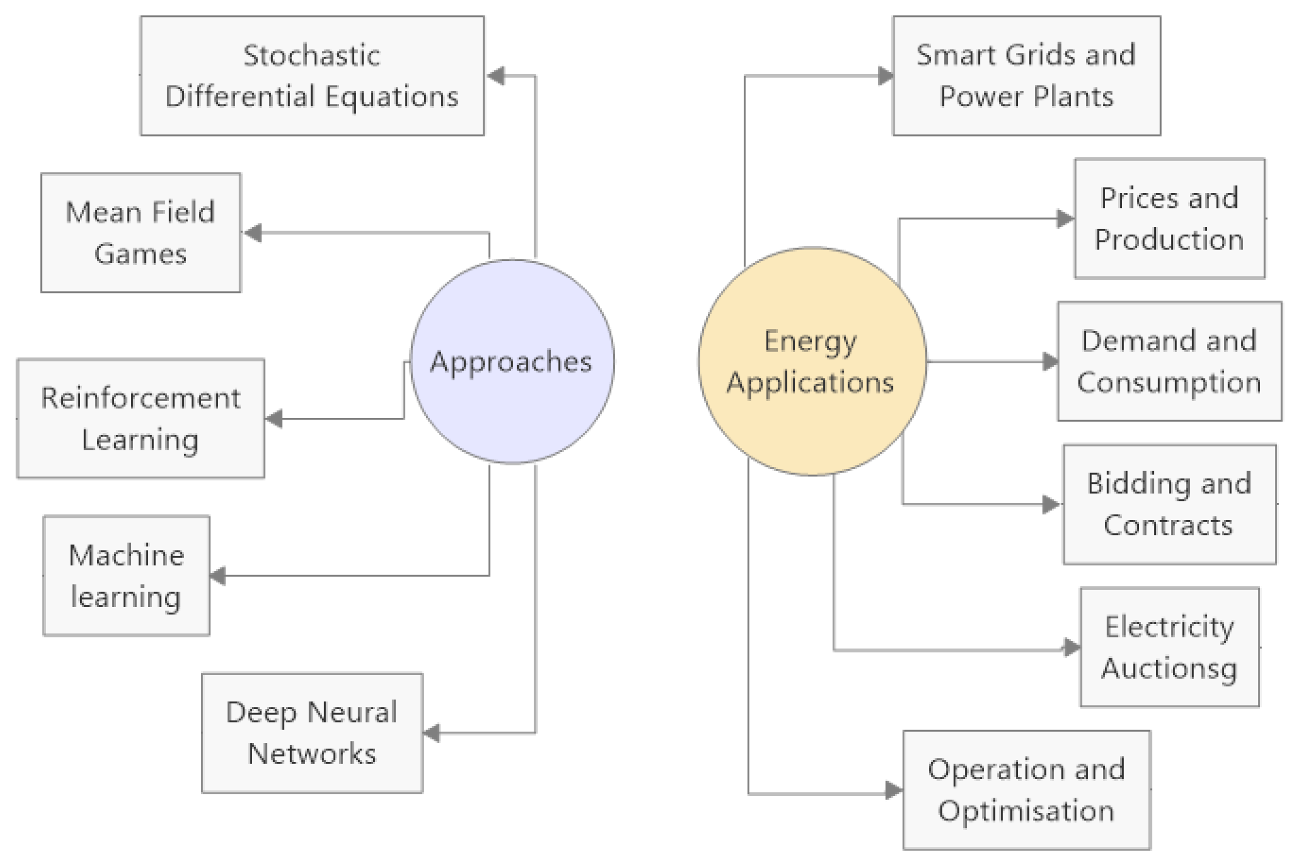