Article

Coordinated Optimization of Multi-Regional Integrated Energy Service Providers with Flexible Reserve Resources

by
Xueting Wang
1,2,*,
Hao Zhong
1,2,
Xianqiu Zou
3,
Qiujie Wang
1,2 and
Lanfang Li
1,2
1
Hubei Provincial Key Laboratory for Operation and Control of Cascaded Hydropower Station, China Three Gorges University, Yichang 443002, China
2
College of Electrical Engineering & New Energy, China Three Gorges University, Yichang 443002, China
3
State Grid Hunan Electric Power Co., Ltd. Loudi Power Supply Company, Loudi 417000, China
*
Author to whom correspondence should be addressed.
Energies 2025, 18(2), 284; https://doi.org/10.3390/en18020284
Submission received: 15 December 2024 / Revised: 4 January 2025 / Accepted: 8 January 2025 / Published: 10 January 2025
(This article belongs to the Special Issue Electricity Market Modeling Trends in Power Systems)

Abstract

:
Aiming at solving the problem of new energy and load uncertainty leading to a steep increase in the demand for flexible reserve resources by integrated energy service providers (IESPs), a coordinated and optimized scheduling method for multi-region integrated energy service providers considering flexible reserve resources is proposed. First, for the uncertainty of new energy and load, Latin hypercube sampling is used to generate scenarios, and the scenarios are reduced by a K-means clustering algorithm. Second, based on the interaction relationship between the active distribution network (ADN) and multi-region IESPs, a mixed game model of the ADN and IESP alliance is established. ADN guides IESPs to optimize their operation by setting prices for electricity and reserves, and IESPs fully tap their own flexible reserve resources according to the prices set by ADN and achieve power interoperability through the interaction of IESPs in multiple regions to synergistically cope with the uncertainties of new energy and load. Finally, the example results show that the model proposed in this paper is able to realize the allocation of flexibility resources in a wider range, reduce the reserve pressure on the superior grid, and improve the profitability of IESPs.

1. Introduction

In recent years, in response to the “dual-carbon” policy, renewable energy sources such as wind power and photovoltaic have been developing rapidly in China [1]. However, the uncertainty of wind and solar power output has adversely affected the safe and stable operation of the power system, resulting in a steep increase in the system’s demand for flexible reserve resources [2,3]. Against this backdrop, integrated energy service providers (IESPs) with multi-energy coupling equipment have gradually become the focus of research in the energy industry [4,5,6]. Multi-regional interconnected IESPs can combine multiple energy conversion devices with demand response to synergize against the impact of source-load uncertainty. The reserve capacity is closely related to the operating status of the energy supply units, and the reserve should be co-optimized with the scheduling plans of IESPs. Therefore, it is of great significance to study the ADN scheduling strategy containing multi-region IESPs, establish a mixed game model of ADN and IESPs, fully tap the reserve resources of IESPs to realize inter-region power interconnection, and explore the best way for IESPs to reduce the reserve pressure on the higher-level grid.
At present, many scholars have conducted research on the reserves of integrated energy systems. Ref. [7] improves the flexibility of generating units by considering the participation of energy storage in reserve configurations with the objective of coping with the risk of source-load uncertainty. Ref. [8] stores the excess thermal energy generated by combined heat and power (CHP) through thermal storage, thus increasing the supply of reserve capacity to the system by the CHP. Ref. [9] suggests that the reserve provided by CHP and fuel cells in integrated energy systems can cope with uncertainty risks. Incentive demand response (IDR) plays an auxiliary role in undertaking the reserve task of the system, but the above literature mainly studies the reserve provided by generating units with energy storage and does not consider the introduction of IDR to reduce the reserve pressure on conventional units. Ref. [10] analyzes how incentivized demand response providing reserve reduces the number of costly units turned on and improves the economics of the system. Ref. [11] addresses the problem of insufficient reserve in the system after wind power is connected to the grid by considering incentive-based demand response to provide reserve, which enhances the system’s ability to consume wind power. Although the above literature considers coping with the uncertainty of new energy sources through reserve capacity, it is only studied for a single region and does not consider that multiple regions have complementarity. Therefore, it is of great significance to consider IESPs containing flexibility resources such as CHP and energy storage to trade with ADNs, to explore the flexibility potential of inter-regional energy flow interactions, and to realize cross-region reserve support to promote the consumption of wind and solar energy.
Multi-regional interconnection systems can synergistically dispatch resources in each region, improve energy utilization, and promote the consumption of new energy sources [12,13,14,15]. Among the existing studies on inter-regional interconnection, Ref. [16] considers multi-energy coupling devices and inter-regional energy mutualization to enhance the wind and solar energy consumption of IESPs. Ref. [17] investigates the trading of electrical and thermal energy between IESPs to achieve the coordinated scheduling of multiple energy sources. Ref. [18] investigates the simultaneous participation of multi-regional integrated energy systems in the interaction of multiple energy sources in order to improve energy utilization. For IESPs to participate in the scheduling of active distribution network (ADN), the two belong to a unity of opposites, and the master–slave game usually studies decision-making interactions among multiple players, where the leader and the follower coordinate with each other to eventually reach a steady state, providing an effective framework for solving multiple complex situations. Ref. [19] develops a two-layer game model for active distribution networks and integrated energy systems, and it verifies that the proposed model can improve the peak shaving and valley filling ability of distribution networks. However, the uncertainty of the source load adversely affects the reliability of power supply of the distribution network and integrated energy system. Most of the above studies deal with the interests of IESPs from the perspective of the master–slave game or cooperative game, respectively, but only considering the master–slave game leads to the impossibility of realizing the overall efficiency optimization of ADNs containing multi-region IESPs. If only the cooperative game is considered, the IESPs are unable to exert active regulation. Therefore, it is of great significance to study the mixed game model under the simultaneous participation of ADNs and multi-regional IESPs in the electricity and reserve markets, so as to improve the economic efficiency of IESPs and ADNs.
Based on this, this paper proposes a coordinated optimal scheduling method for multi-regional IESPs considering flexible reserve resources. A hybrid game model is constructed, i.e., the master–slave game for the ADN and IESP alliance and the cooperative game for the IESP alliance. ADNs guide IESPs to optimize the operation by setting the price of electricity and reserve, and the IESPs fully exploit their own flexible reserve resources according to the price set by ADNs, so that the CHP combined with thermal storage and gas boilers can realize thermoelectric decoupling and, through the interaction of the multi-regional IESPs, realize power interconnection. Case analysis shows that the proposed model is able to realize the flexibility resource allocation in a wider range, reduce the reserve pressure of the superior grid, and improve the profitability of IESPs.

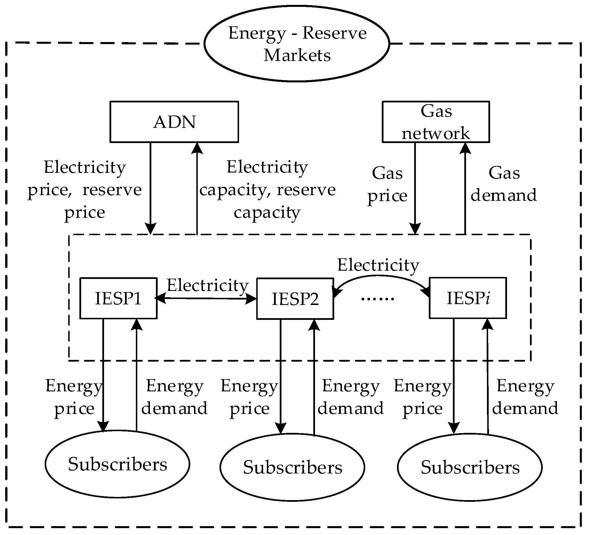
2. Participation of IESPs in Energy and Reserve Market Trading Mechanisms

IESPs can provide users with a full range of energy services, such as electricity, heat, and natural gas, and develop a reasonable plan to improve energy utilization based on users’ energy use [20]. The structure of the IESPs considered in this paper is shown in Figure 1, and its internal CHP can be combined with a gas boiler and a heat storage tank to realize thermoelectric decoupling, so as to provide a flexible reserve for the system. IDR is characterized by flexible response and rapid regulation [21]. Energy storage devices can respond quickly to changes in demand and adjust the output power flexibly. Therefore, CHP, IDR, and energy storage devices can all provide reserve capacity to the system.
The energy trading framework in this paper is shown in Figure 2, where the ADN can purchase electricity and reserve capacity from both the higher-level grid and the coalition of IESPs, while regional IESPs purchase natural gas from the natural gas grid to supply energy, and the heat load is supplied by internal CHP and gas boilers. The ADN sets the price of electricity and reserve capacity from the coalition of IESPs, and when there is an excess of electricity in IESPs, it will be sold to the members of coalition who do not have enough electricity, and the excess will be traded to the ADN. When the IESPs have a surplus of electricity, they first sell it to the members of the alliance that have a surplus of electricity and then trade the surplus with the ADN. When the IESPs have a shortage of electricity, they first buy it from the members of the alliance that have a surplus of electricity and then buy the shortage from the ADN.

3. ADN and IESPs Alliance Mixed Game Model

The master–slave game can help the leader to optimize the incentive mechanism, so that the followers can make decisions that are consistent with the master’s goals while maximizing their interests. ADN-coordinated scheduling containing multi-region IESPs is a complex multi-interest subject scheduling strategy problem, where the ADN sets energy prices, the lower IESPs respond according to the prices, there are sequences and leadership between the two, and the master–slave game is usually adopted. Therefore, this paper establishes a hybrid game model based on the relationship between an ADN and IESPs, i.e., the master–slave game of an ADN and IESP alliance and the cooperative game of the IESP alliance.
ADN, as the leader of the master–slave game, can set the price of electricity and the price of reserve to the coalition of IESPs. IESPs, as the follower of the game, calculate the appropriate trading power and trading tariffs among IESPs based on the price of electricity and reserve set by the ADN. The appropriate inter-alliance transaction price ensures that the IESPs make a profit, and the ADN then trades with the higher-level grid based on the power and reserve capacity purchased by the IESP alliance.

3.1. Gaming Leader ADN

3.1.1. Objective Function of ADN

An ADN aims to minimize the sum of its own purchased power and reserve costs as follows:
min F ADN = t = 1 24 π w w = 1 n w ( C IESP , t , w + C UG , t , w )
C IESP , t , w = i = 1 M ( u e , i , t b P i , t , w b , IESP + u r , i , t b , ur P i , t , w b , IESP , ur + u r , i , t b , dr P i , t , w b , IESP , dr u e , i , t s P i , t , w s , IESP u r , i , t s , ur P i , t , w s , IESP , ur u r , i , t s , dr P i , t , w s , IESP , dr )
C UG , t , w = λ e , t b P t , w b , UG + λ r , t b , ur P t , w b , UG , ur + λ r , t b , dr P t , w b , UG , dr
where π w is the occurrence probability of scenario w; C IESP , t , w and C UG , t , w are the transaction costs of the ADN–IESP alliance and superior power grid under scenario w at time t, respectively; u r , i , t , w b , ur and u r , i , t , w b , dr are the up-reserve prices and down-reserve prices of the purchase made by the ADN to IESP i under scenario w at time t; u r , i , t , w s , ur and u r , i , t , w s , dr are, respectively, the up-reserve prices and down-reserve prices sold by the ADN to IESP i under scenario w at time t; u e , t , w b and u e , t , w s are the purchase and sale prices set by the ADN for IESP i under scenario w at time t; and P i , t , w b , IESP , ur and P i , t , w b , IESP , dr are the up-reserve capacity and down-reserve capacity purchased by the ADN from IESP i in scenario w at time t. P i , t , w s , IESP , ur and P i , t , w s , IESP , dr are the up-reserve capacity and down-reserve capacity sold by the ADN to IESP i under scenario w at time t; P i , t , w b , IESP and P i , t , w s , IESP are the power capacity purchased and sold by the ADN to IESP i under scenario w at time t; λ e , t b , λ r , t s , ur , and λ r , t s , dr are showing that ADN buys power from the superior grid at time t, the up-reserve price, and the down-reserve price; and P t , w b , UG , P t , w b , UG , ur , and P t , w b , UG , dr are the power purchased from the upper power grid in scenario w at time t, the up-reserve capacity, and the down-reserve capacity.

3.1.2. ADN Constraints

(1)
The power balance constraint is as follows:
P t , w L + i = 1 M P i , t , w s , IESP = P t , w b , UG + P t , w new + i = 1 M P i , t , w b , IESP
where P t , w L and P t , w new are the ADN load and new energy predicted value under scenario w at time t.
(2)
Reserve capacity constraints are as follows:
P t , w b , UG , ur + i = 1 M P i , t , w b , IESP , ur P ADN , t ur + i = 1 M P i , t , w s , IESP , ur
P t , w b , UG , dr + i = 1 M P i , t , w b , IESP , dr P ADN , t dr + i = 1 M P i , t , w s , IESP , dr
where P ADN , t ur and P ADN , t dr are the up-reserve requirements and down-reserve requirements of the ADN at time t.

3.2. Game Follower IESPs Alliance

3.2.1. Objective Function of the IESPs Alliance

The objective function is the i integrated energy service provider with the greatest economic benefit:
max U i IESP = t = 1 24 π w w = 1 n w ( C ADN , i , t , w + C i , t , w trad C i , t , w g C ES , i , t , w C TS , i , t , w C DR , i , t , w C R , i , t , w )
where C ADN , i , t , w is the income of IESP i and the ADN trading power and reserve under scenario w at time t, C i , t , w trad is the income from the purchase and sale of electric energy between IESP i and other regions under scenario w at time t, C i , t , w g is the cost of natural gas purchased by IESP i under scenario w at time t, C ES , i , t , w and C TS , i , t , w are the costs of IESP i electric and thermal energy storage under scenario w at time t, C DR , i , t , w is the cost of IESP i demand response under scenario w at time t, and C R , i , t , w is the spare capacity cost of IESP i under scenario w at time t.
C i , t , w trad = j = 1 j i M ( p i j , t e q i j , t , w e )
C ES , i , t , w = C E , i P i , t , w e , ES
C TS , i , t , w = C T , i P i , t , w h , TS
C DR , i , t , w = λ IDR , i e P i , t , w e , IDR + λ IDR , i h P i , t , w h , IDR + λ IDR , i g P i , t , w g , IDR + λ PDR , i e P i , t , w e , PDR + λ PDR , i h P i , t , w h , PDR + λ PDR , i g P i , t , w g , PDR
C R , i , t , w = C IDR , i , t ur R IDR , i , t , w ur + C IDR , i , t dr R IDR , i , t , w dr + C CHP , i , t ur R CHP , i , t , w ur + C CHP , i , t dr R CHP , i , t , w dr + C ES , i , t ur R ES , i , t , w ur + C ES , i , t dr R ES , i , t , w dr
where p i j , t e is the electricity price traded between IESP i and IESP j , q i j , t , w e is the power capacity traded between IESP i and IESP j under scenario w at time t, C E and C T are the charge and discharge cost coefficients of electric and thermal energy storage, P i , t , w e , ES and P i , t , w h , TS are the charge and discharge power of electric and thermal energy storage under scenario w at time t, λ IDR , i e is the cost factor of interruptible electrical load in IESP i , P i , t , w e , IDR is the load that IESP i can interrupt under scenario w at time t, C IDR , i , t ur and C IDR , i , t dr are the cost coefficients of IDR up-adjustment and down-adjustment of reserve capacity in IESP i at time t, and R IDR , i , t , w ur and R IDR , i , t , w dr are the up-reserve capacity and down-reserve capacity provided by IDR in IESP i in scenario w at time t.

3.2.2. Constraints of the IESPs Alliance

(1)
The power balance constraint is as follows:
P i , t , w b + P i , t , w new + P i , t , w e , IDR + P i , t , w e , CHP + P i , t , w in , ES = P i , t , w s + P i , t , w out , ES + P i , t , w e , load + j = 1 j i M q i j , t , w
P i , t , w h , CHP + P i , t , w h , GB + P i , t , w h , IDR + P i , t , w h , TS , out = P i , t , w h , TS , in + P i , t h , load
P i , t , w g , ub + P i , t , w g , IDR = P i , t , w g , CHP + P i , t , w g , GB + P i , t g , load
where P i , t , w new is the new energy output of IESP i under scenario w at time t, P i , t , w b is the electric energy purchased by IESP i from the ADN under scenario w at time t, P i , t , w e , CHP is the electric energy generated by CHP in IESP i under scenario w at time t, P i , t , w h , GB is the heat energy generated by GB in IESP i under scenario w at time t, P i , t , w in , ES and P i , t , w out , ES are the charging and discharging energies of ES in scenario w at time t, and P i , t , w e , load , P i , t , w h , load , and P i , t , w g , load are the power of electricity, heat, and gas load after price-type demand response in IESP i under scenario w at time t.
(2)
The demand response constraint is as follows:
P PDR e , max P i , t , w e , PDR P PDR e , max
t = 1 24 P i , t , w e , PDR = 0
0 P i , t , w e , IDR u i , t , w P IDR e , max
where P PDR e , max is the maximum transferable electrical load of IESP i , is the interrupt state of interruptible load in IESP i under scenario w in time period t, P IDR e , max is the maximum interruptible electrical load of IESP i . Regarding the heat load and gas load demand response constraint cocurrent load, this article will not go into more detail.
(3)
The IDR reserve constraints are as follows:
0 R i , t , w IDR , dr P i , t , w e , IDR
0 R i , t , w IDR , ur u i , t , w P IDR e , max P i , t , w e , IDR
where R i , t , w IDR , ur and R i , t , w IDR , dr are the up-reserve and down-reserve provided by interruptible power load under scenario w at time t in IESP i , respectively.
(4)
The constraints on energy storage devices are as follows:
0 P i , t , w CH P CH max I s , t , w
0 P i , t , w DC P DC max I r , t , w
I s , t , w + I r , t , w 1
S e , t , w = S e , t 1 , w + [ P i , t , w CH η e CH P i , t , w DC / η e DC ]
S e min S e , t , w S e max
S e , 0 , w = S e , T , w
where P CH max and P DC max are the maximum charge and discharge power of energy storage; I s , t , w and I r , t , w are the charging and discharging state variables of ES under scene w at time t; η e CH and η e DC are charging and discharging efficiency, respectively; and S e , t , w is the ES capacity in scenario w at time t. Thermal energy storage constraints are the same as those for electric energy storage, which will not be described here.
(5)
The constraints on CHP are as follows:
P i , t , w e , CHP = η i , e CHP P i , t , w g , CHP
P i , t , w h , CHP = η i , h CHP P i , t , w g , CHP
0 P i , t , w e , CHP P CHP , i e , max I CHP , i , t , w
0 P i , t , w h , CHP P CHP , i h , max I CHP , i , t , w
P i , t , w e , CHP P i , t 1 , w e , CHP r CHP , i up ( 1 u CHP , i , t , w ) + r CHP , i down u CHP , i , t , w
P i , t , w e , CHP P i , t 1 , w e , CHP r CHP , i down ( 1 v CHP , i , t , w ) + r CHP , i down v CHP , i , t , w
where η i , e CHP and η i , h CHP are the conversion coefficients of electric power and thermal power of CHP in IESP i , respectively. P CHP , i e , max and P CHP , i h , max are, respectively, the maximum electrical and thermal power outputs of CHP in IESP i . I CHP , i , t , w is the on–off state of the CHP in IESP i under scenario w at time t, u CHP , i , t , w and v CHP , i , t , w are the state quantities of CHP on and off in IESP i under scenario w at time t, and r C H P , i down and r C H P , i up are, respectively, the upper and lower limits of the climb rate of CHP in IESP i .
(6)
The gas boiler constraints are as follows:
P i , t , w h , GF = η i GF P i , t , w g , GF
0 P i , t , w h , GF P GF , i h , max
where P i , t , w h , GF is the heat energy generated by the gas boiler at time t and scenario w, η i GF is the thermal power conversion coefficient of the gas-fired boiler, P i , t , w g , GF is the natural gas power input by GF in IESP i under scenario w at time t, and P GF , i max is the maximum thermal power output of GF in IESP i .
(7)
The reserve constraints of the unit are as follows:
0 R i , t , w CHP , ur min [ P CHP , i e , max I CHP , i , t , w P i , t , w e , CHP , r CHP , i up I CHP , i , t , w ]
0 R i , t , w CHP , dr min [ P i , t , w e , CHP P CHP , i e , min I CHP , i , t , w , r CHP , i down I CHP , i , t , w ]
0 R t , w ES , ur min { [ S e , t , w S e min ] η e DC , P DC max P DC , t , w }
0 R i , t , w ES , dr min { [ S e max S e , t , w ] / η e CH , P CH max P CH , t , w }
(8)
The reserve capacity constraints are as follows:
R i , t , w ES , ur + R i , t , w CHP , ur + R i , t , w IDR , ur R i , t , w b , IESP , ur + R i , t , w s , IESP , ur R i , t ur
R i , t , w ES , dr + R i , t , w CHP , dr + R i , t , w IDR , dr R i , t , w b , IESP , dr + R i , t , w s , IESP , dr R i , t dr
where R i , t ur and R i , t dr are the up-reserve and down-reserve demand of IESP i at time t.

3.3. IESP Alliance Nash Negotiation Model

Nash negotiation can effectively describe the cooperative interaction between alliance members. In this paper, the Nash negotiation model is used to ensure that all members of the alliance can reach the Pareto equilibrium solution.
max i = 1 M ( U i U i 0 ) s.t.       U i U i 0
where U i is the benefit obtained by IESP i from participating in the negotiation, while U i 0 is the benefit obtained by IESP i from not participating in the negotiation.
However, this model is difficult to solve directly, so it is divided into two sub-problems: alliance benefit maximization (P1) and cooperation benefit distribution (P2).

3.3.1. SubProblem (P1) Maximization of Alliance Profits

max U IESP = i = 1 M π w w = 1 n w t = 1 24 ( C ADN , i , t , w C i , t , w g C ES , i , t , w C TS , i , t , w C DR , i , t , w C R , i , t , w ) s.t. Formulas 7 40
where U IESP is revenue from alliance cooperation.

3.3.2. Subproblem (P2) Distribution of Cooperation Profits

max i = 1 M ln [ ( t = 1 24 j = 1 j i M ( p i j , t e q i j , t e * ) + U i IESP * ) U i 0 ] s . t . t = 1 24 j = 1 j i M ( p i j , t e q i j , t e * ) + U i IESP * U i 0 u e , i , t s * p i j , t e u e , i , t b * U i IESP * = t = 1 24 π w w = 1 n w ( C ADN , i , t , w C i , t , w g C ES , i , t , w C TS , i , t , w C DR , i , t , w C R , i , t , w )
where the variable marked with * is the optimal solution to maximize the benefits of the alliance. U i IESP * is the benefit of IESP i obtained via the maximization of the alliance benefit.

4. Model Solving

4.1. Uncertain Scenario Portrayal for Wind, PV, and Loads

Aiming at overcoming the uncertainty of wind power, PV, and load output, this paper adopts Latin hypercubic sampling to generate a large number of wind power, photovoltaic, and load output scenarios obeying probability distributions. The Latin hypercube sampling method, a stratified and dimensional random sampling method, enables the sampling points to be distributed as much as possible throughout the sampling space, effectively overcoming the phenomenon of truncation, thus improving the sampling accuracy and efficiency.
Taking wind power as an example, suppose ( P 1 , P 2 ,⋯, P t ) is the historical output data of wind power for t hours in a day and ( Δ P 1 , Δ P 2 ,⋯, Δ P t 1 ) is the incremental data of wind power output, i.e., Δ P t = P t + 1 P t . F(x) is the cumulative probability distribution function of wind power output incremental data for a typical day, and let N be the sampling size; the specific steps are described as follows.
(1)
The cumulative probability distribution function F(x) into N non-overlapping sub-intervals, each spaced 1/N apart.
(2)
t−1 random numbers in the range [0, 1], denoted by r t m , at each equal portion m. Calculate the value of the cumulative probability function corresponding to each random number as follows: p t m = ( 1 / N ) r t m + ( t 1 ) / N .
(3)
The incremental sampling value of wind power data x t m is obtained according to the inverse function F 1 ( p t m ) of the cumulative probability distribution function, i.e.: x t m = F 1 ( p t m )
(4)
The historical output data are added to the incremental sampling values obtained in step (3) to simulate the generation of wind power output data.
(5)
If the obtained randomized scenario m has negative power at moment t, i.e., p t m < 0 , then take p t m = 0 .
(6)
An N × t-dimensional matrix is generated to randomly order the data in each column, i.e., N random wind power outflow scenarios are generated.
Consider that if all scenario sets are used for calculation, it will have a great impact on the calculation speed. In order to reduce the calculation time and obtain representative photovoltaic and load data for the following research, scene reduction technology is needed. K-means clustering algorithm can efficiently process multi-dimensional and large-scale data and achieve a quick reduction in scenes. Typical scenarios obtained after the reduction are shown in Appendix A The steps are as follows:
(1)
The cluster number W 0 was determined, and W 0 samples were randomly selected as initial cluster centers.
(2)
The Euclidean distance between each sample and each cluster center is calculated and compared. The nearest cluster center is the cluster to which the sample belongs.
(3)
All samples in the same cluster are averaged as the new cluster center coordinates for the cluster
(4)
Steps (2) and (3) repeat the calculation until all in-cluster samples no longer change.
(5)
The probability of the occurrence of each scene is calculated, with π w , π w representing the number of scenes in the wth category divided by the total number of scenes.

4.2. Solving Master–Slave Game Based on KKT Condition

In the master–slave game of the ADN and IESP alliance, due to the coupling of the iteration process and complex trading strategy, the model presents strong nonlinearity and non-convexity, so the global optimal solution cannot be obtained directly. In order to enable commercial solvers to solve it directly, the advantage of the KKT condition in optimization problems is used to convert bilevel problems into monolayer mixed integer linear programming problems.
The master–slave game process of the ADN and IESP alliance considered in this paper is carried out in the following steps:
Step 1: ADN sets prices for the purchase and sale of electricity and reserve to IESPs;
Step 2: IESPs respond according to the ADN’s power and reserve prices and its own output and feedback the purchase and sale of power and reserve plans to the ADN;
Step 3: The ADN revises the prices again based on the plans reported by the IESPs for the purchase and sale of power and reserve capacity.

4.3. Solving Cooperative Game Based on ADMM

The transaction prices of IESP i and IESP j are coupled to each other. In order to ensure that the interaction prices between IESPs are equal, the coupling variables need to be decoupled, that is, the following:
p i j , t e = p j i , t e = z i j , t e
ADMM can decompose complex problems into multiple sub-problems and simplify the calculation process by using a single-variable solution. Compared to the centralized problem, decentralized using ADMM, the scheduling problem not only ensures the independence and privacy of the different producers and consumers but also enhances the scalability of the proposed model by reducing the computation time of the energy management of the micro-energy network operator. So, we take the inverse of the objective function and solve the model through ADMM. The IESP i distributed optimization models obtained by decomposition are as follows:
min L i = ln [ U i 0 ( t = 1 24 ( p i j , t e q i j , t e * ) + U i * ) ] + t = 1 24 j = 1 , j i M ω i j , t ( p i j , t e z i j , t e ) + ρ 2 p i j , t e z i j , t e 2 2 s.t. t = 1 24 ( p i j , t e q i j , t e * ) + U i * U i 0 u e , i , t s * p i j , t e u e , i , t b *
where ω i j , t is the dual variable interacting from IESP i to IESP j , while ρ is the penalty factor.
( p i j , t , k + 1 e ) = arg min L i ( p i j , t , k e , z i j , t , k e , ω i j , t , k )
( p j i , t , k + 1 e ) = arg min L i ( p j i , t , k e , z i j , t , k e , ω i j , t , k )
where k is the number of iterations, while ω i j , t , k is the dual variable of the KTH iteration.
The transaction price of electric energy between the k + 1 IESP, obtained from Equations (46) and (47), updates the auxiliary variable of the price of k + 1:
z i j , t , k + 1 e = ( p i j , t , k + 1 e + p j i , t , k + 1 e ) / 2
From the price auxiliary variable of k + 1, we find the dual variable of k + 1:
ω i j , t , k + 1 = ω i j , t , k + ρ ( p i j , t , k + 1 e + z i j , t , k + 1 e ) / 2
The convergence conditions is as follows:
t = 1 24 p i j , t , k + 1 e z i j , t , k + 1 e 2 2 ε
where ε is the coefficient of convergence.

5. Example Analysis

The clearing price of power from the upper power grid is shown in Table 1, the parameters related to IESPs are shown in Table 2, and the interruptible and transferable load does not exceed 10% of the initial load. The experiments in this paper were conducted using MATLAB version 9.5.0.944444, GUROB version 9.0.3 and MOSEK version 9.3.12 as a learning framework. For subproblem (P1), programming and solving were performed using MATLAB and GUROBI, with a computational time of about 425s; for subproblem (P2), programming and solving were performed using MATLAB and MOSEK, with a computational time of about 25s.

5.1. Each Subject Transaction Price Analysis

The electricity prices set by the ADN and the electricity prices traded between IESPs are shown in Figure 3.
ADN, in order to ensure its own revenue, sets its power purchase tariffs to the IESP Union higher than the power sales tariffs. During 01:00–06:00 and 23:00–24:00, ADN wind power generation is larger, and users use less electricity, at which time the ADN is in the net load valley time, and the valley time tariff is established. During 07:00–09:00, 15:00–17:00, and 21:00–22:00, the difference between the ADN’s new energy output and its load is not big, and it is in the net load usual period, so the usual tariff is set. During the hours of 10:00–14:00 and 18:00–20:00, the net load of ADN is at its peak, and the peak tariff is set. IESPs, in order to ensure the benefit of cooperation, always trade at a price lower than the price of purchasing electricity from the ADN and higher than the price of selling electricity to the ADN, so the IESPs in each region prioritize inter-regional trading and then trade the remaining electricity with the ADN. It is also because the members of each IESPs consortium have the ability to set their own prices, so they can have better bargaining power with the ADN while protecting the interests of each member. It can be seen that cooperative gaming reduces the dependence of IESPs on the ADN and improves the operational efficiency.

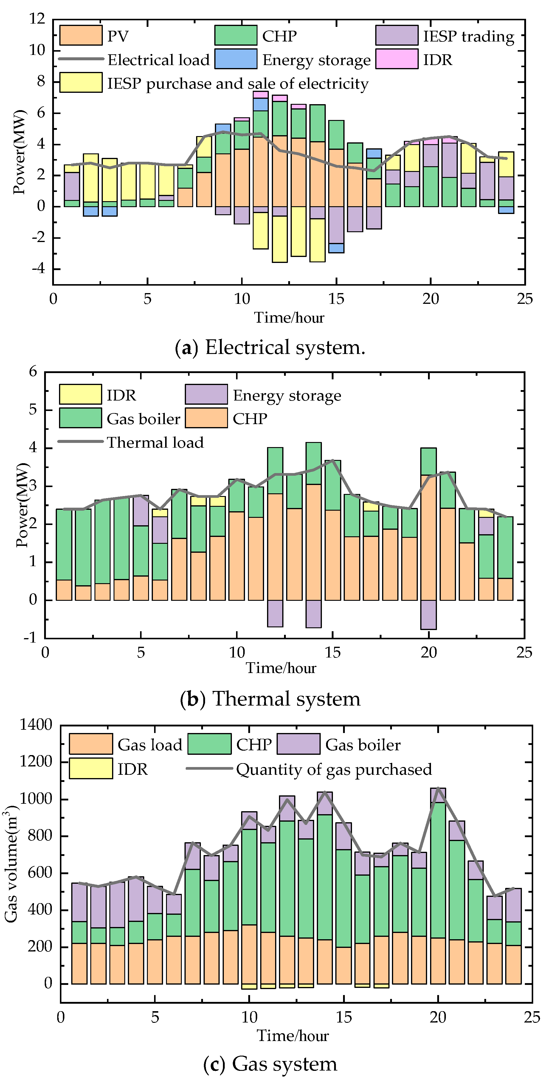
5.2. Analysis of Electrical, Heat, and Gas Balance Results

The optimization results of IESP1 are shown in Figure 4. During the 01:00–06:00 and 23:00–24:00, the ADN sets a lower price for electricity and there is no output from PV, and there is a surplus of wind generation from IESP3. IESP1 prioritizes the purchase of electricity from IESP3 in order to reduce the operating costs and buys the shortfall from the ADN. IESP1 needs to cope with the problem of the uncertainty in the source loads, so the CHP needs to keep the output small to provide reserve for IESP1. In the flat price period set by the ADN, the CHP maintains a high-output operation from 07:00 to 09:00, 15:00 to 17:00 and 21:00 to 22:00. The heat load is satisfied by the heat production of CHP and the gas boiler. The CHP produces more heat, and the gas boiler operates at a smaller output and realizes the thermoelectric decoupling of CHP, so that the CHP can provide up-reserve and down-reserve. During the peak price period set by the ADN, from 10:00 to 14:00 and from 18:00 to 20:00, the system interrupts part of the electrical load, and at the same time, the electric energy storage and discharge are provided to reduce the reserve pressure of the system, and the CHP maintains a higher unit output, so as to obtain greater profits by selling electric energy in the electricity market. CHP generate excess heat energy that is stored through heat storage tanks. Among them, from 10:00 to 14:00, IESP1 produces a photovoltaic power generation surplus, in order to absorb new energy, to sell electricity to IESP3 from 18:00 to 20:00, because IESP1’s CHP output is limited and photovoltaic power generation is 0, so buying electricity from IESP3 is avoided. The analyses of IESP2 and IESP3 are similar to this stage and are therefore not repeated in this paper.

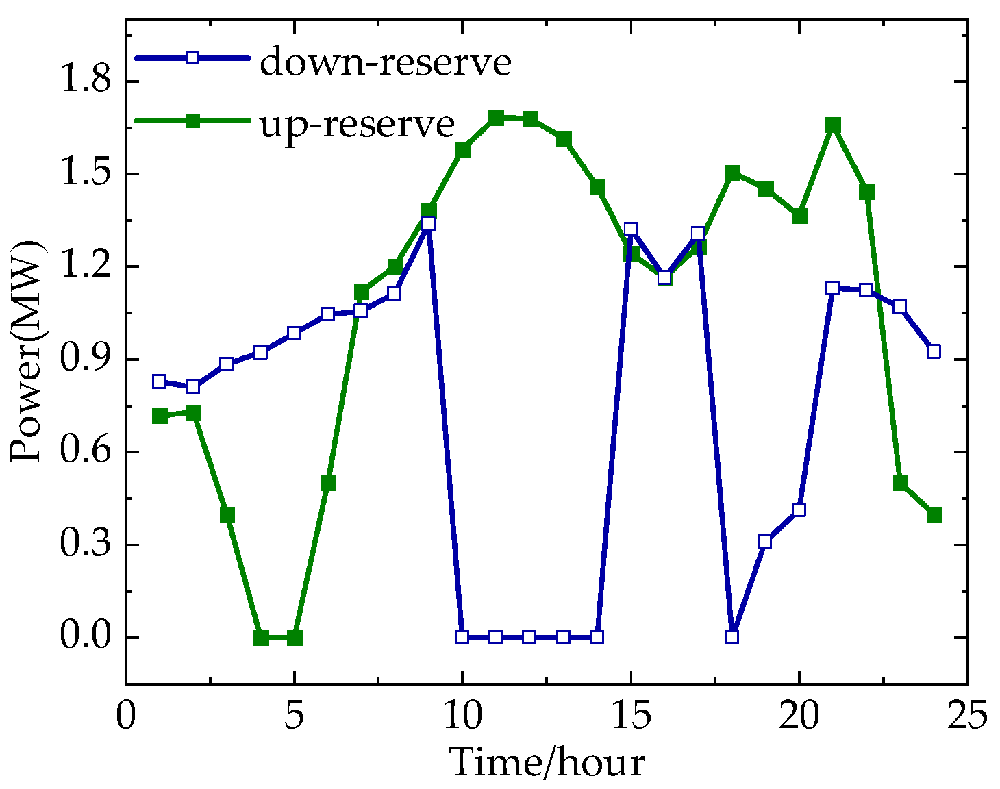
5.3. Analysis of Reserve Capacity Optimization Results

Figure 5 shows the reserve provided by energy storage, IDR, and CHP. In the figure, it can be seen that after considering the multiple flexible reserve resources, the reserve provided by the CHP remains dominant, and energy storage and IDR play a supplementary role in undertaking the reserve task of the system. During the peak tariff hours set by the ADN, IDR can curtail the peak load, which is equivalent to a virtual power supply replacing the CHP output. In addition, the CHP’s ability to provide reserve during peak hours is weak and inadequate, so considering IDRs to provide rotating reserve relieves the CHP’s reserve pressure The up-reserve provided by energy storage at peak tariffs reduces the reserve pressure on CHP, thus allowing CHP to maintain high output levels while coping with wind, photovoltaic, and load uncertainty. The reserve provided by energy storage is also taken into account when developing the energy storage charging and discharging plan, which gives full recognition to the role of energy storage. When the electricity price is low, CHP power output is low and gas boiler maintains higher output, and when electricity price is high, CHP maintains higher power output and the gas boiler maintains lower output. Therefore, considering thermal energy storage and the gas boiler enables CHP thermoelectric decoupling, which not only provides electricity to the electricity market but also provides reserve to the rotating reserve market, which increases the economic efficiency of IESP1.

5.4. Analysis of Alternate Transaction Results Between ADN and IESPs

Figure 6 shows the reserve capacity sold by the IESPs to the ADN. During the low tariff hours set by the ADN for the IESPs, the CHP is less productive and therefore provides less down-reserve capacity, while the down-reserve capacity provided by the storage units and the CHP is essentially used to cope with fluctuations in their own wind loads, and therefore the IESPs sell less down-reserve capacity and more up-reserve capacity to the ADN. During the high tariff hours set by the ADN to the IESPs, the CHP operates at higher outputs and thus provides less up-reserve, and the up-reserve provided by electric storage, IDR, and CHP is essentially used to cope with fluctuations in their own wind loads, so the IESPs sell less up-reserve and more down-reserve to the ADN.

5.5. Scheme Comparison Analysis

In order to verify the effectiveness of the scheme proposed in this paper, four schemes are set up for comparative analysis:
Scheme 1: Consider the cooperation game between IESPs and demand response, which is the method proposed in this paper;
Scheme 2: Ignore the cooperation game between IESPs and consider demand response;
Scheme 3: Consider the cooperation game between IESPs without considering the demand response;
Scheme 4: Do not consider the cooperation game between IESPs and do not consider the demand response.

5.5.1. Economic Benefit Analysis of IESPs Under Each Scheme

The economic benefits of IESPs under different schemes are shown in Table 3 and defined below:
(1)
An analysis of the effectiveness of cooperative game: Compared with the scheme 2, scheme 1 considers the cooperative game, and the income of the IESs alliance in the first scheme is 4842 yuan higher than in the second scheme. This is due to the fact that the trading of electricity between IESP members utilizes inter-regional complementarities, which reduces the dependence of IESPs on the ADN and achieves an increase in the total benefits of the IESP alliance. Compared with directly trading with the ADN, the benefits for each IESP increased by 1337 yuan, 779 yuan, and 2726 yuan, respectively.
(2)
Demand response effectiveness analysis: Compared with scheme 3, it can be found that scheme 1 considers more incentive demand response and price demand response, which increases the revenue of each IESP alliance by 877 yuan, 1110 yuan, and 1083 yuan. This is because IESPs can transfer or cut the load when the price of electricity is high. At the same time, the implementation of incentive demand response increases the reserve capacity of IESPs, effectively relieves the reserve pressure of CHP, and improves the economy of system operation.
(3)
The effectiveness analysis of the cooperative game and demand response is also considered: Compared with scheme 4, scheme 1 considers the cooperation game and demand response, which makes the income of IESPs in each region in scheme 1 increase by 2204 yuan, 1862 yuan, and 3973 yuan, respectively. This is due to the fact that the price of electricity traded between regions is higher than the price of electricity supplied to the ADN. IDR has a short response time to reduce or stop electricity consumption during peak tariffs. When the IESPs have sufficient power, the IESPs provide more power to the ADNs and thus the IESPs increase their revenues.Through the comparison of the above schemes, it is found that the mixed game model of the IESP and ADN alliance considering flexible reserve resources proposed in this paper can effectively improve the economic benefits of each region.

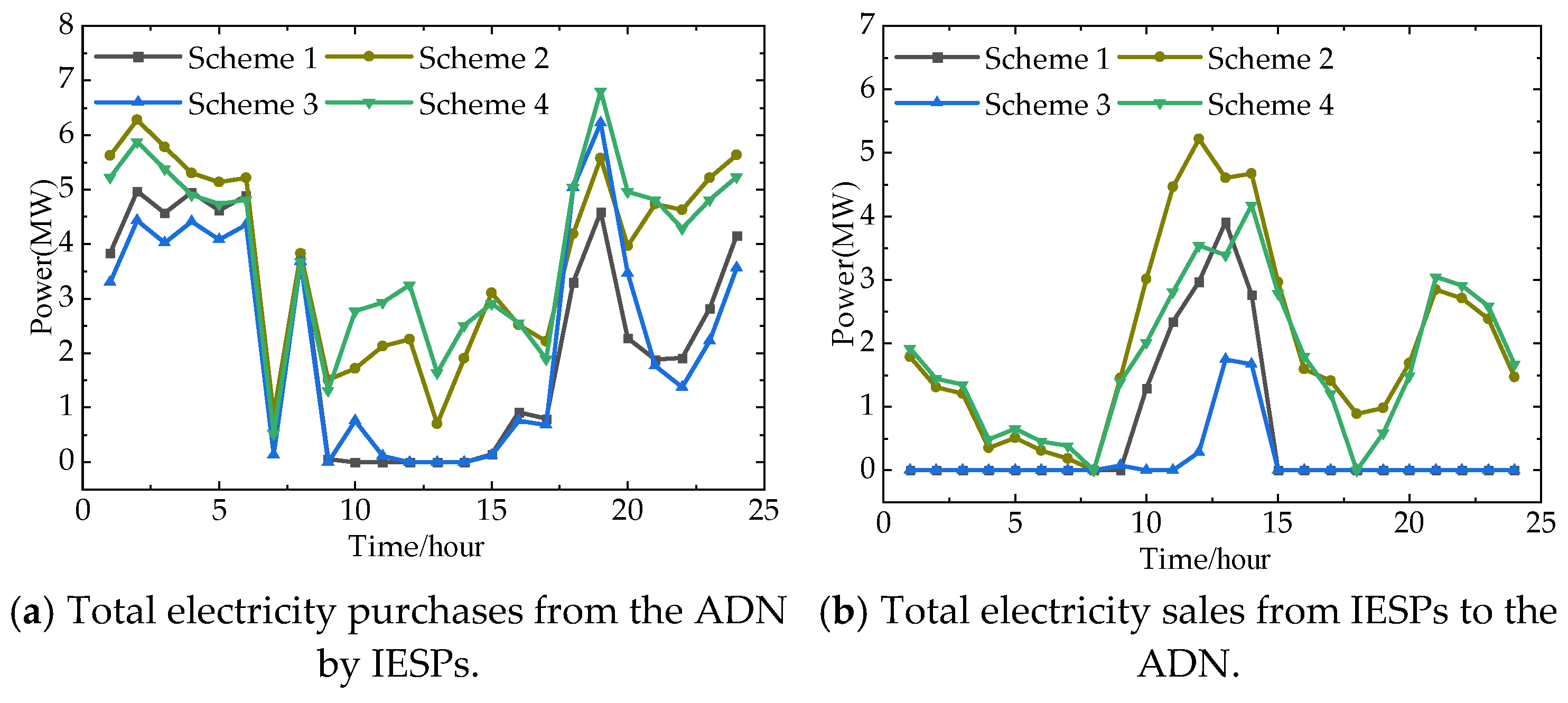
5.5.2. Analysis of Total Transaction Power of IESPs and the ADN Under Each Scheme

Figure 7 shows the total electricity purchased and sold by IESPs to the ADN under the four schemes. Compared with scheme 1, scheme 2 does not consider the cooperation game, and the purchased and sold electric energy of IESPs depend on the ADN, so the total electric energy purchased from and sold to the ADN by IESPs is more in scheme 2. Scheme 4 also has more total purchases and sales of electricity from IESPs to the ADN in compared to scheme 3, because scheme 4 does not consider cooperative gaming. It can be seen that considering cooperative gaming reduces the dependence of the IESPs on the ADN. In the case of scheme 3, demand response is not considered, so in the period of low electricity prices set by the ADN from the IESP alliance, the IESP alliance in scheme 3 buys less electric energy from the ADN, and in the period of high electricity prices set by the ADN from the IESP alliance, the IESP alliance in scheme 3 sells less electric energy to the ADN. It can be seen that after taking demand response into account, IESPs can transfer or cut the electrical load when the electricity price is high, thereby reducing the operating cost.

6. Conclusions

This paper takes the ADN and multi-regional IESPs as the research object, comprehensively considers the reserve capacity required by the ADN and IESPs in the face of uncertainty, and builds a mixed game model, which is in line with the actual interests of multi-agents. The main conclusions are as follows:
(1)
The mixed game model established in this paper takes into account the uncertainty of new energy and load and collaboratively formulates the unit output plan and reserve capacity scheme of IESPs in each region, as well as the trading power among the subjects. ADN formulates the price of electricity and reserve to guide the IESPs to fully exploit their own flexible reserve resources, alleviate the pressure of reserve on the higher-level grids, and enhance the profitability of the IESPs.
(2)
Cooperative gaming can coordinate the scheduling of IESP resources in each region and reduce the dependence on the ADN. Compared to trading directly with ADN, the benefits of each regional IESP are increased by 1337 yuan, 779 yuan, and 2726 yuan, respectively.
(3)
The example simulation results show that the flexible reserve resources provided by energy storage and demand response participate in system optimal scheduling, which can improve the flexibility of the CHP group operation and thus improve the economy of system operation. In addition, the method proposed in this paper can provide a reference point for integrated energy systems with large new energy installed capacity and encourage more flexible resources to provide reserve.

Author Contributions

Conceptualization, X.W. and H.Z.; methodology, X.W.; software, X.W. and L.L.; validation, X.Z. and H.Z.; formal analysis, X.W.; investigation, Q.W.; resources, X.W.; data curation, L.L.; writing—original draft preparation, X.W.; writing—review and editing, H.Z. All authors have read and agreed to the published version of the manuscript.

Funding

This research was funded by the National Natural Science Foundation of China, grant number 52307109.

Data Availability Statement

The original contributions presented in this study are included in the article; further inquiries can be directed to the corresponding author.

Acknowledgments

This research was supported by Hao Zhong’s group at China Three Gorges University. We deeply appreciate their diligent work and contribution.

Conflicts of Interest

Author Xianqiu Zou was employed by the company State Grid Hunan Electric Power Co., Ltd. Loudi Power Supply Company. The remaining authors declare that the research was conducted in the absence of any commercial or financial relationships that could be construed as a potential conflict of interest.

Nomenclature

P CHP e , max Maximum electrical power output of combined heat and power
η i , h CHP Thermal power conversion factor for combined heat and power
η i , e CHP Electrical power conversion factor for combined heat and power
r CHP , i up Maximum creep rate for combined heat and power
r CHP , i down Minimum creep rate for combined heat and power
C E , i Costs of charging and discharging electrical energy storage
C T , i Charge and discharge costs for thermal energy storage
P CH e , max Maximum charging power of electrical energy storage
P DC e , max Maximum discharge power of electric energy storage
S e max Maximum capacity of electrical energy storage
S e min Minimum capacity of electrical energy storage
λ IDR e Electric load demand response costs
λ IDR h Thermal load demand response costs
λ IDR g Gas load demand response costs
P GF h , max Maximum thermal power output of gas boiler
η GF Thermal power conversion factor for gas boiler
π w Probability of occurrence of scenario w
ρ Penalty factor
ε Convergence factor

Abbreviations

IESPIntegrated energy service provider
ADNActive distribution network
IDRIncentive demand response
CHPCombined heat and power
PVPhotovoltaic
WTWind turbine
KKTKarush–Kuhn–Tucker
ADMMAlternating direction multiplier method

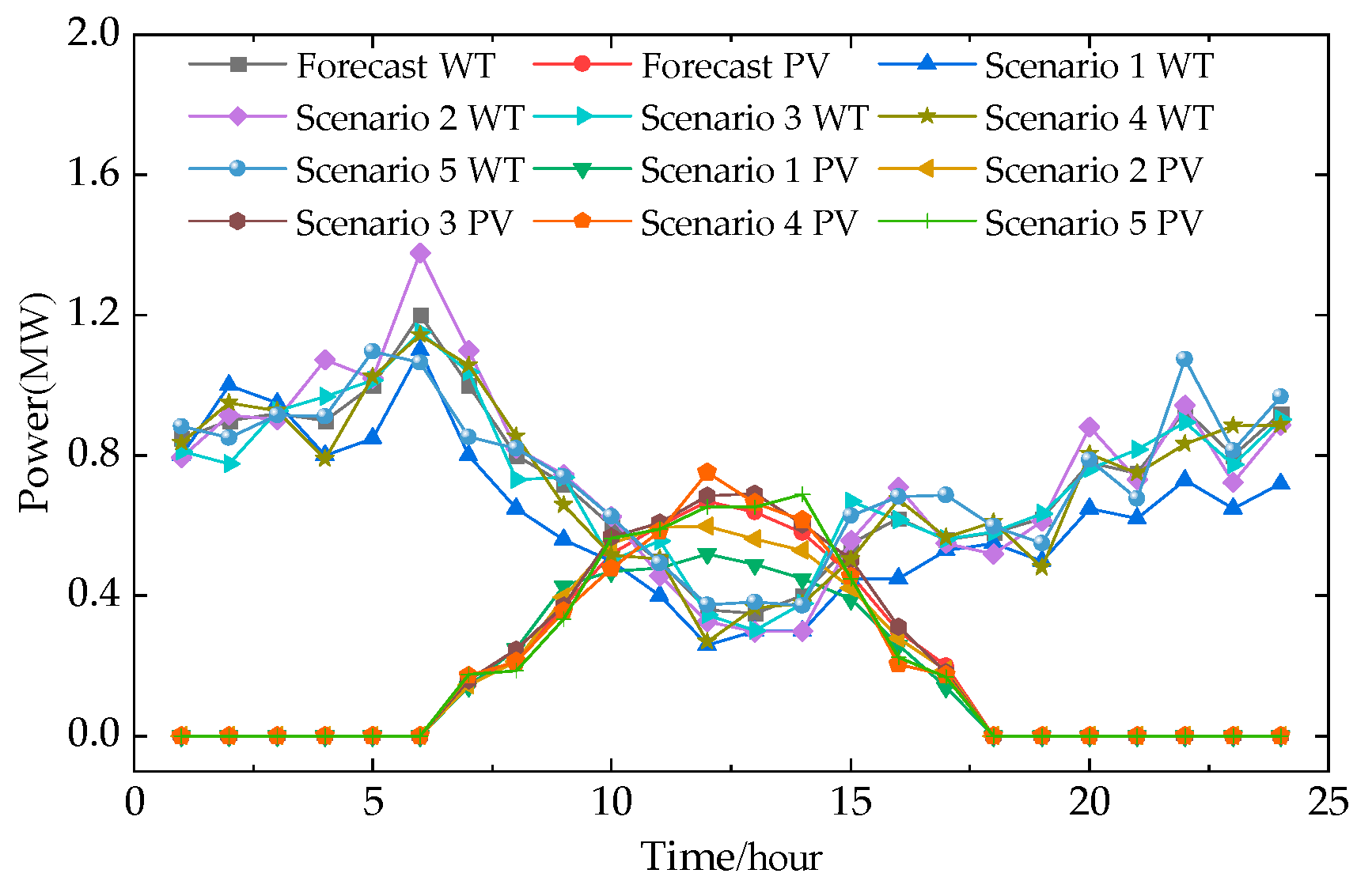
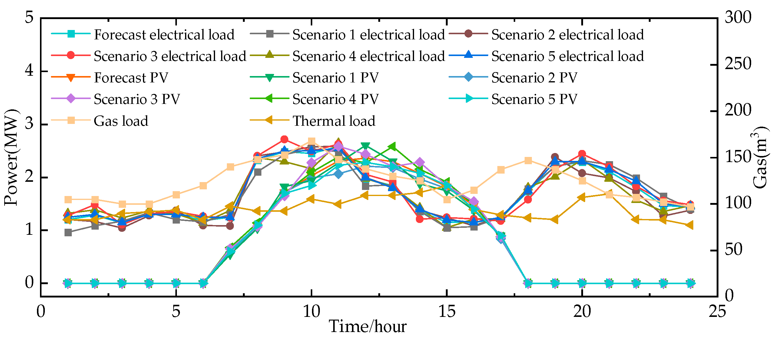
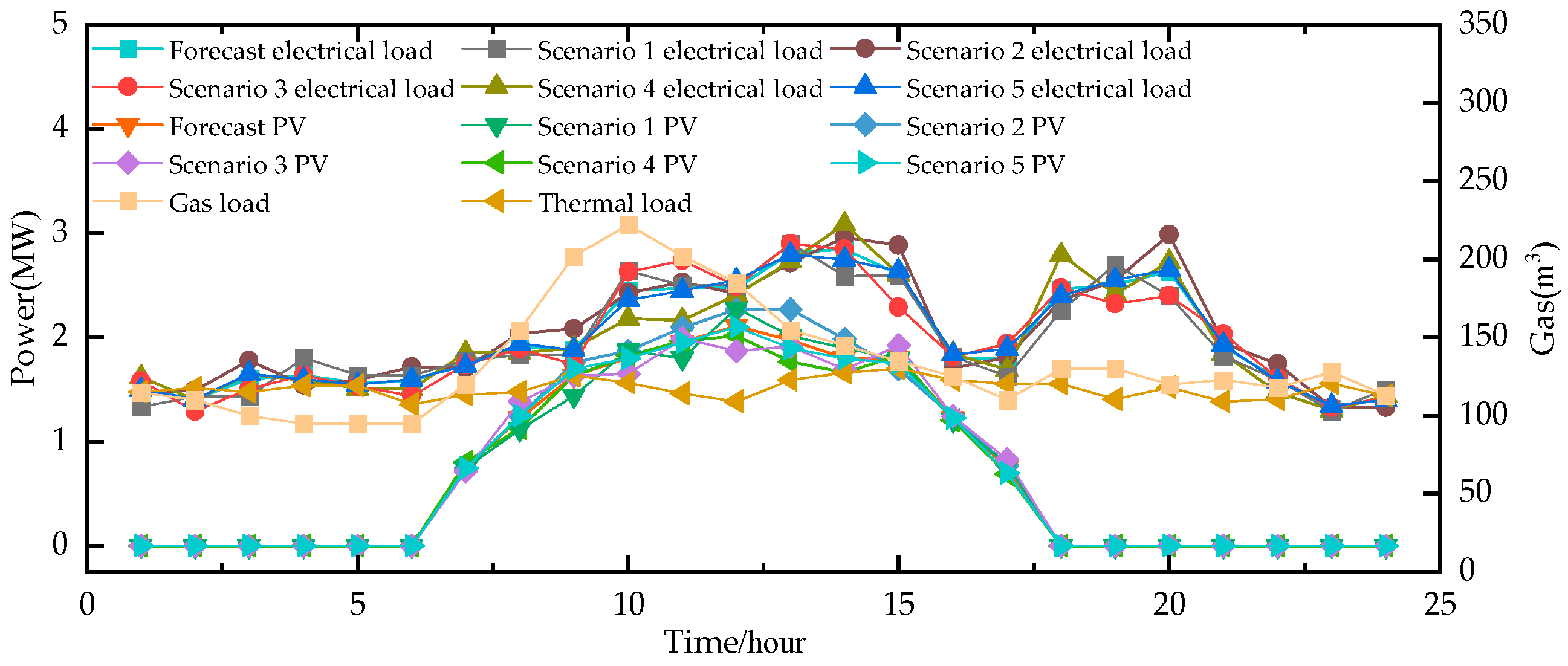
Appendix A. WT, PV, and Load-Out Scenarios

Figure A1. WT and PV output scenarios in ADN.
Energies 18 00284 g0a1
Figure A2. Load-out scenarios in ADN.
Energies 18 00284 g0a2
Figure A3. Load and PV output scenarios in IESP1.
Energies 18 00284 g0a3
Figure A4. Load and PV output scenarios in IESP2.
Energies 18 00284 g0a4
Figure A5. Load and WT output scenarios in IESP1.
Energies 18 00284 g0a5

References

  1. Wang, K.; Niu, D.; Yu, M.; Liang, Y.; Yang, X.; Wu, J.; Xu, X. Analysis and countermeasures of China’s green electric power development. Sustainability 2021, 13, 708. [Google Scholar] [CrossRef]
  2. Safaei, M.; Al Dawsari, S.; Yahya, K. Optimizing Multi-Channel Green Supply Chain Dynamics with Renewable Energy Integration and Emissions Reduction. Sustainability 2024, 16, 9710. [Google Scholar] [CrossRef]
  3. Mohandes, B.; Moursi, M.S.E.; Hatziargyriou, N.; Khatib, S.E. A Review of power system flexibility with high penetration of renewables. IEEE Trans. Power Syst. 2019, 34, 3140–3155. [Google Scholar] [CrossRef]
  4. Lu, Q.; Guo, Q.; Zeng, W. Optimization scheduling of integrated energy service system in community: A bi-layer optimization model considering multi-energy demand response and user satisfaction. Energy 2022, 252, 124063. [Google Scholar] [CrossRef]
  5. Luo, F.; Shao, J.; Jiao, Z.; Zhang, T. Research on optimal allocation strategy of multiple energy storage in regional integrated energy system based on operation benefit increment. Int. J. Electr. Power Energy Syst. 2021, 125, 106376. [Google Scholar] [CrossRef]
  6. Lu, Q.; Guo, Q.; Zeng, W. Optimization scheduling of an integrated energy service system in community under the carbon trading mechanism: A model with reward-penalty and user satisfaction. J. Clean. Prod. 2021, 323, 129171. [Google Scholar] [CrossRef]
  7. Nasrolahpour, E.; Kazempour, J.; Zareipour, H.; Rosehart, W.D. A Bilevel Model for Participation of a Storage System in Energy and Reserve Markets. IEEE Trans. Sustain. Energy 2018, 9, 582–598. [Google Scholar] [CrossRef]
  8. Zhou, Y.; Hu, W.; Min, Y.; Dai, Y. Integrated Power and Heat Dispatch Considering Available Reserve of Combined Heat and Power Units. IEEE Trans. Sustain. Energy 2019, 10, 1300–1310. [Google Scholar] [CrossRef]
  9. Yang, R.; Li, K.; Liu, J.; Liu, J.; Xiang, Y. Day-ahead Economic Dispatch Model of Park Integrated Energy System Considering Reserve Allocation of Energy Storage. Electr. Power Constr. 2022, 43, 103–111. [Google Scholar]
  10. Li, N.; Sun, S.; Zhang, L.; Wang, J.; Qu, Y. The Evaluation Method of the Power Supply Capability of an Active Distribution Network Considering Demand Response. Processes 2024, 12, 2719. [Google Scholar] [CrossRef]
  11. Chen, Z.; Li, F.; Huang, R. Spinning reserve optimal configuration strategy of a wind power system with demand response. Power Syst. Prot. Control. 2020, 48, 117–122. [Google Scholar]
  12. Mo, L.; Deng, Z.; Chen, H.; Lan, L. Multi-Objective Co-Operative Game-Based Optimization for Park-Level Integrated Energy System Based on Exergy-Economic Analysis. Energies 2023, 16, 7945. [Google Scholar] [CrossRef]
  13. Ji, X.; Li, M.; Li, M.; Han, H. Low-carbon dispatch of multi-regional integrated energy systems considering integrated demand side response. Front. Energy Res. 2024, 12, 1361306. [Google Scholar] [CrossRef]
  14. Sun, H.; Zou, H.; Jia, J.; Shen, Q.; Duan, Z.; Tang, X. Master–Slave Game Optimization Scheduling of Multi-Microgrid Integrated Energy System Considering Comprehensive Demand Response and Wind and Storage Combination. Energies 2024, 17, 5762. [Google Scholar] [CrossRef]
  15. Yang, S.; Tan, Z.; Lin, H.; De, G.; Zhou, F. Stochastic Optimization and Income Allocation Model for Park Integrated Energy System Considering Cooperation Alliance. Power Syst. Autom. 2020, 44, 36–46. Available online: https://link.cnki.net/urlid/32.1180.TP.20200713.1548.008 (accessed on 3 January 2025).
  16. Cui, M.; Xuan, M.; Lu, Z.; He, L. Operation Optimization Strategy of Multi Integrated Energy Service Companies Based on Cooperative Game Theory. Proc. CSEE 2022, 10, 3548–3564. [Google Scholar] [CrossRef]
  17. Zhou, C.; Zheng, C.B. Energy Trading Strategy for Heat and Electricity-Coupled Microgrid Based on Cooperative Game. Appl. Sci. 2022, 12, 6568. [Google Scholar] [CrossRef]
  18. Khazaei, H.; Aghamohammadloo, H.; Habibi, M.; Mehdinejad, M.; Mohammadpour Shotorbani, A. Novel Decentralized Peer-to-Peer Gas and Electricity Transaction Market between Prosumers and Retailers Considering Integrated Demand Response Programs. Sustainability 2023, 15, 6165. [Google Scholar] [CrossRef]
  19. Tong, X.; Hu, C.; Zheng, C.; Rui, T.; Wang, B.; Shen, W. Energy Market Management for Distribution Network with a Multi-Microgrid System: A Dynamic Game Approach. Appl. Sci. 2019, 9, 5436. [Google Scholar] [CrossRef]
  20. Lai, X.; Xie, Z.; Xu, D.; Ying, S.; Zeng, Y.; Jiang, C.; Wang, F.; Wen, F.; Palu, I. Operation Optimization of an Integrated Energy Service Provider with Ancillary Service Provision. Energies 2022, 15, 4376. [Google Scholar] [CrossRef]
  21. Cui, Y.; Deng, G.; Zhao, Y.; Zhong, W.; Tang, Y.; Liu, X. Economic Dispatch of Power System With Wind Power Considering the Complementarity of Low-carbon Characteristics of Source Side and Load Side. Proc. CSEE 2021, 41, 4799–4815. [Google Scholar] [CrossRef]
Figure 1. Integrated energy service provider.
Energies 18 00284 g001
Figure 2. Energy trading framework.
Energies 18 00284 g002
Figure 3. Member transaction prices.
Energies 18 00284 g003
Figure 4. Electricity, thermal, and gas balance results in IESP1.
Energies 18 00284 g004
Figure 5. Flexibility resource participation reserve optimization decision result in IESP1.
Energies 18 00284 g005
Figure 6. IESP selling of reserve to the ADN.
Energies 18 00284 g006
Figure 7. Total electricity purchases and sales by IESPs to the ADN.
Energies 18 00284 g007
Table 1. Electricity price of upper network.
Time FramePrice (Yuan/kW·h)
Valley time01:00–06:00; 23:00–24:000.25
Flat price period07:00–09:00; 15:00–17:00; 21:00–22:000.58
Rush hour10:00–14:00; 18:00–20:001
Table 2. Parameters related to IESPs.
ParametersNumerical ValueParametersNumerical Value
P CHP e , max /MW2 η i , e CHP /(kW/m3)3.5
η i , h CHP /(kW/m3)4.5 r CHP , i up /(MW/h)0.8
r CHP , i down /(MW/h)0.8 C E , i /(yuan/kW·h)0.01
P CH e , max /(MW/h)0.6 P DC e , max /(MW/h)0.6
S e max /(MW·h)2 S e min /(MW·h)0.3
P CH h , max /(MW/h)0.4 P DC h , max /(MW/h)0.4
S h max /(MW·h)1.5 S h min /(MW·h)0.2
P GF h , max /MW2 η GF /(kW/m3)9
λ IDR , 1 e /(yuan/kW·h)0.5 λ IDR , 2 e /(yuan/kW·h)0.48
λ IDR , 3 e /(yuan/kW·h)0.48 λ IDR h /(yuan/kW·h)0.25
λ IDR g /(yuan/kW·h)0.25 C T , i /(yuan/kW·h)0.005
λ PDR e /(yuan/kW·h)0.08 λ PDR h /(yuan/kW·h)0.05
λ PDR g /(yuan/kW·h)0.05
Table 3. A comparison of the benefits of IESPs under four schemes.
SchemeIESP1 Earnings
(Ten Thousand Yuan)
IESP2 Earnings
(Ten Thousand Yuan)
IESP3 Earnings
(Ten Thousand Yuan)
Total Earnings
(Ten Thousand Yuan)
1−3.1096−3.8904−4.9612−11.9612
2−3.2433−3.9683−5.2338−12.4454
3−3.1973−4.0015−5.0695−12.2683
4−3.3300−4.0766−5.3585−12.7651
Disclaimer/Publisher’s Note: The statements, opinions and data contained in all publications are solely those of the individual author(s) and contributor(s) and not of MDPI and/or the editor(s). MDPI and/or the editor(s) disclaim responsibility for any injury to people or property resulting from any ideas, methods, instructions or products referred to in the content.

