Analytical Computation of the Maximum Power Point of Solar Cells Using Perturbation Theory

Abstract

To compute the maximum power point (MPP) from physical parameters of the single-diode model (SDM), it is necessary to solve a transcendental equation using numerical methods. This is computationally expensive and can lead to divergence problems. An alternative is to develop analytical approximations which can be accurate enough for engineering problems and simpler to use. Therefore, this paper presents approximations for computing the MPP of single-junction solar cells. Two special cases are considered: (i) SDM with only series resistance, and (ii) SDM with only shunt resistance. Power series closed-form expressions for the MPP are obtained using perturbation theory and the Lagrange inversion theorem. Validation of the formulas is performed using experimental data from six different technologies obtained from the NREL database and comparing the results with the numerical solution of the SDM and three approximations from the literature. The results show an absolute percentage error (APE) of less than 0.035% with respect to the real MPP measurements. In cases with limited computational resources, this value could be further improved by using a higher- or lower-order power-series approximation.

1. Introduction

Shockley’s diode equation describes the behavior of the electrical variables of an ideal solar cell. In order to include the power losses experienced by an operating solar cell, the resistance of the series $R_{\mathrm{s}}$ and the shunt $R_{\mathrm{p}}$ need to be included through Kirchhoff’s current law (KCL) and Ohm’s laws [1]. The resulting model is commonly referred to as the five-parameter single-diode model (SDM) [2]. In this case, an implicit equation arises when calculating the current–voltage ($I-V$) characteristic, which is necessary to solve numerically. Banwell et al. showed [3] that an explicit expression for the current in terms of the voltage that includes $R_{\mathrm{s}}$ can be obtained with the Lambert $\mathrm{W}$-function. A version of this expression that also includes $R_{\mathrm{p}}$ was developed in [4]. In [5], formulas were presented for computing the voltage in terms of the current and explicit expressions for short-circuit current $I_{\mathrm{sc}}$ and open-circuit voltage $V_{\mathrm{oc}}$.

The maximum power point (MPP) voltage $V_{\mathrm{mpp}}$ and current $I_{\mathrm{mpp}}$ are the pair of points of an $I-V$ curve for which the power defined by $P=VI$ is at its maximum. The MPP is of interest because commercial solar panels are optimized to operate at this point for better efficiency [6]. Furthermore, the MPP used as a simulation tool for predicting generation power [7], estimating the MPP in real time using low-cost hardware [8], or calculating the power density for optimal flow studies [9], to mention only a few applications. The MPP computation problem has been addressed from different approaches. In [10], the Lagrange multiplier method was used, employing an objective function to maximize the power within the constraint of satisfying the $I-V$ equation of the photovoltaic (PV) module. A similar methodology was used in [11], with the addition of an objective function to maximize the rectangle inside the $I-V$ characteristic curve and study of the double diode model. In [12], the objective was to maximize the power output using the tilt angle of the PV module given an arbitrary location, which was accomplished through the use of neural networks. Using measurements of the slope of the $I-V$ curve around points $I_{\mathrm{sc}}$ and $V_{\mathrm{oc}}$, ref. [13] constructed a parallelogram by which the MPP was computed using Lagrangian interpolation. Through the use of Thevenin and Norton equivalent circuits, ref. [14] approximated a linearized version of the $I-V$ curve of the PV module around the MPP in order to relate the parameters of the equivalent circuits to a variety of weather conditions. On the other hand, a significant problem in PV cell modeling consist of finding an explicit expression for the MPP in terms of the physical parameters of the SDM. Numerical method can be employed to easily determine the MPP with arbitrary accuracy; however, these methods are computationally expensive and may have divergence problems if the initial value is relatively far from the exact value of the solution. Therefore, it is worth finding analytical expressions for $I_{\mathrm{mpp}}$ and $V_{\mathrm{mpp}}$ with an acceptable level of accuracy. These should allow for quick and easy calculation of the MPP.

Obtaining analytical expressions is based on simplifications that reduce the implicit transcendental equation to an analytically solvable one. The previous literature has addressed this calculation from different approaches. The problem of including only $R_{\mathrm{s}}$ was first tackled in [15] provided an explicit expression describing the relationship between voltage and current. From this expression, they proceeded to derive formulas for calculating $V_{\mathrm{mpp}}$ and $I_{\mathrm{mpp}}$. Subsequently, expressions for MPP voltage and current were obtained in [8] through analytical methods based on the Mean Value Theorem (MVT) applied to the implicit current equation. Building on this, in [16] the Lambert W-function was employed to refine the PV module’s current equation. It was observed that the arguments of the Lambert W-function take on small values, allowing for an approximation in which these terms are replaced by their arguments to simplify the expressions for $V_{\mathrm{mpp}}$ and $I_{\mathrm{mpp}}$. The resulting equations can be analytically solved using the Lambert W-function, providing a more precise approach. The problem of solving the transcendental equation for the MPP becomes more complex when $R_{\mathrm{p}}$ is included in the formulation. This problem was initially addressed in [17], where the problem was reduced to a quadratic equation for $I_{\mathrm{mpp}}$ by employing some simplifications (such as $V_{\mathrm{mpp}}/R_{\mathrm{p}}\to 0$ and $\frac{\mathrm{d}V}{\mathrm{d}I}/R_{\mathrm{p}}\to 0$) and using a linear approximation to solve the problem analytically. In [7,18], the exact solution of the MPP for the ideal case was presented in terms of the Lambert $\mathrm{W}$-function. The parameters $R_{\mathrm{p}}$ and $R_{\mathrm{s}}$ were included using the KCL. An alternative approach for analytical computation of the MPP was presented in [19], where an explicit model with parameters associated with the SDM was taken as a reference. Returning to the idea of applying the MVT to the $I-V$ curve, ref. [20] applied the MV to the ideal SDM to find an approximation for the MPP, which was dependent on the natural logarithm and included $R_{\mathrm{s}}$ and $R_{\mathrm{p}}$ by viewing the circuit as a two-port network. Recently, the exact solution to the problem of applying the MVT to MPP computation was finally found in [21].

It is well known that the accuracy of MPP calculation is strongly dependent on the method used to calculate the SDM parameters. In [22], the authors found that with available $I-V$ curve measurements, the most accurate method for representing curve is presented in [23], which considers the five-parameter SDM. When data sheet information is available, the most accurate approach is presented in [24,25], which uses the so-called simplified SDM. This model neglects either $R_{\mathrm{p}}$ or $R_{\mathrm{s}}$ depending on the value of the series-parallel coefficient (SPR) parameter. In the case of SPR $>1$, only $R_{\mathrm{s}}$ is considered and $R_{\mathrm{p}}\to \infty$; otherwise if SPR $<1$, then $R_{\mathrm{s}}=0$, and a finite value of $R_{\mathrm{p}}$ is taken. In the current literature there is no approximation for the latter case, only the model where $R_{\mathrm{s}}$ or a combination of $R_{\mathrm{s}}$ and $R_{\mathrm{p}}$ are considered; nevertheless, the expressions obtained in this way lack accuracy due to the multiple simplifications.

In this work, analytical approximations of these two special cases are developed using perturbation theory and the Lagrange inversion theorem (LIT). For the case in which only $R_{\mathrm{s}}$ is considered, an implicit equation for $I_{\mathrm{mpp}}$ obtained from the SDM is converted into the dimensionless form $u(a,\gamma )$, where a and $\gamma$ are dimensionless parameters. From here, we note that for small values of a (which correspond to small values of $R_{\mathrm{s}}$), it is possible to obtain an analytical closed-form expression for u. Using perturbation theory, it can be argued that this approximation is close to the exact solution, at least at a small distance $\xi$. Expanding the power series around $\xi$ = 0, an expression for the exact form is found using the LIT. For the other case, where $R_{\mathrm{p}}$ is considered, a similar methodology is followed, using the $V_{\mathrm{mpp}}$ estimate of the ideal case as an initial approximation. The expressions are validated using the set of six $I-V$ curves measured by the NREL and presented in [26], where they are found to have an error of less than 0.035%.

2. Problem Description

Assuming nondegenerate conditions, the total current I produced by a solar cell follows Shockley’s diode equation [27]. When series and shunt resistance are considered, this equation becomes

$$I=I_{\mathrm{L}}-I_0\left(exp\left(\alpha (V+I{R}_{\mathrm{s}})\right)-1\right)-\frac{I{R}_{\mathrm{s}}+V}{R_{\mathrm{p}}},$$

(1)

where

$$\alpha =\frac{q}{A{N}_s{k}_{\mathrm{B}}T},$$

with $N_s$ being the number of cells connected in series, T the module temperature, $k_{\mathrm{B}}$ Boltzmann’s constant, q the electron charge, A the ideality factor of the diode, $I_0$ the recombination current, $I_{\mathrm{L}}$ the photogeneration current, $R_{\mathrm{s}}$ the series resistance, and $R_{\mathrm{p}}$ the shunt resistance. From Equation (1), the implicit solutions for the current in terms of the voltage (and vice versa) follow [5]

$$\begin{array}{cc}\hfill I& =\frac{\left(I_{\mathrm{L}}+I_0\right)R_{\mathrm{p}}-V}{R_{\mathrm{p}}+R_{\mathrm{s}}}-\frac{\mathrm{W}\left({\mathcal{F}}_{\mathrm{I}}\right)}{\alpha R_{\mathrm{s}}},\hfill \end{array}$$

(2)

$$\begin{array}{cc}\hfill V& =\left(I_{\mathrm{L}}+I_0\right)R_{\mathrm{p}}-I(R_{\mathrm{s}}+R_{\mathrm{p}})-\frac{1}{\alpha }\mathrm{W}\left({\mathcal{F}}_{\mathrm{V}}\right),\hfill \end{array}$$

(3)

with

$$\begin{array}{cc}\hfill {\mathcal{F}}_{\mathrm{I}}& =\frac{\alpha I_0{R}_{\mathrm{p}}{R}_{\mathrm{s}}}{R_{\mathrm{p}}+R_{\mathrm{s}}}exp\left(\frac{\alpha R_{\mathrm{p}}\left(V+\left(I_{\mathrm{L}}+I_0\right)R_{\mathrm{s}}\right)}{\left(R_{\mathrm{p}}+R_{\mathrm{s}}\right)}\right),\hfill \\ \hfill \end{array}$$

(4)

$$\begin{array}{cc}\hfill {\mathcal{F}}_{\mathrm{V}}& =\alpha I_0{R}_{\mathrm{p}}exp\left(\left(I_{\mathrm{L}}+I_0-I\right)R_{\mathrm{p}}\alpha \right).\hfill \end{array}$$

(5)

At the maximum power point (MPP), it follows that $\frac{\mathrm{d}P}{\mathrm{d}V}=\frac{\mathrm{d}P}{\mathrm{d}I}=0$. The maximum power point voltage $V_{\mathrm{mpp}}$ and current $I_{\mathrm{mpp}}$ follow the implicit forms [21]

$$\begin{array}{cc}\hfill -V_{\mathrm{mpp}}+\frac{R_{\mathrm{p}}{V}_{\mathrm{mpp}}}{\left(R_{\mathrm{p}}+R_{\mathrm{s}}\right)\left(\mathrm{W}\left({\mathcal{F}}_{V_{\mathrm{mpp}}}\right)+1\right)}=& \frac{\mathrm{W}\left({\mathcal{F}}_{V_{\mathrm{mpp}}}\right)}{\alpha }+\frac{R_{\mathrm{s}}{V}_{\mathrm{mpp}}-\left(I_{\mathrm{L}}+I_0\right)R_{\mathrm{s}}{R}_{\mathrm{p}}}{(R_{\mathrm{p}}+R_{\mathrm{s}})},\hfill \\ \hfill \end{array}$$

(6)

$$\begin{array}{cc}\hfill I_{\mathrm{mpp}}\left(\frac{R_{\mathrm{p}}}{\mathrm{W}\left({\mathcal{F}}_{I_{\mathrm{mpp}}}\right)+1}+R_{\mathrm{s}}\right)=& \left(I_{\mathrm{L}}+I_0\right)R_{\mathrm{p}}-I_{\mathrm{mpp}}(R_{\mathrm{p}}+R_{\mathrm{s}})-\frac{1}{\alpha }\mathrm{W}\left({\mathcal{F}}_{I_{\mathrm{mpp}}}\right),\hfill \end{array}$$

(7)

where W(x) is Lambert’s $\mathrm{W}$-function, defined by $x=\mathrm{W}\left(x{e}^x\right)$, and ${\mathcal{F}}_{V_{\mathrm{mpp}}}$ and ${\mathcal{F}}_{I_{\mathrm{mpp}}}$ are Equations (4) and (5) evaluated at $V=V_{\mathrm{mpp}}$ and $I=I_{\mathrm{mpp}}$, respectively. Equations (6) and (7) are transcendental equations that cannot be solved analytically. Numerical methods can then be employed; however, these may present divergence problems and can be computationally expensive. In the following section, analytical approximations are presented to avoid these problems.

3. Mathematical Background

This section presents two mathematical tools employed in the present work to find the analytical approximations of the MPP: perturbation theory and the Lagrange inversion theorem (LIT).

Let $x=x_0$ be the exact root of the equation $f\left(x\right)=0$. Consider the problem of finding the roots of a transcendental equation in the form

$$h(x,\epsilon )=f\left(x\right)+\epsilon g\left(x\right)=0,$$

(8)

where $\epsilon$ is a small parameter satisfying $\left|\epsilon \right|<<1$. Following perturbation theory, the solution to Equation (8) can be expressed as a power series in $\epsilon$ of the following form:

$$x=\sum _{n=0}^{\infty }{x}_n{\epsilon }^n.$$

(9)

Expanding to the first order in $\epsilon$ gives

$$\begin{array}{cc}\hfill x& =x_0+\epsilon x_1+O\left({\epsilon }^2\right),\hfill \end{array}$$

(10)

where $x_1$ is the first-order coefficient of the power series. Standard perturbation theory requires substituting Equation (10) in Equation (8) and collecting terms of equal powers of $\epsilon$. This results in a system of algebraic equations that can be solved analytically. However, in this work we explore a different approach. First, we expand $h(x,\epsilon )$ via Taylor series expansion around $x_0$ to provide

$$h(x,\epsilon )=\sum _{n=0}^{\infty }\frac{h^{\left(n\right)}(x_0,\epsilon )}{n!}{(x-x_0)}^n.$$

(11)

Substituting Equation (10) into Equation (11) and simplifying yields

$$\begin{array}{cc}\hfill h(x,\epsilon )& =\sum _{n=0}^{\infty }\frac{h^{\left(n\right)}(x_0,\epsilon )}{n!}{(x_0+\epsilon x_1-x_0)}^n\hfill \\ \hfill & =\sum _{n=0}^{\infty }\frac{h^{\left(n\right)}(x_0,\epsilon )}{n!}{\left(\epsilon x_1\right)}^n\hfill \\ \hfill & =\sum _{n=0}^{\infty }\frac{h^{\left(n\right)}(x_0,\epsilon ){\epsilon }^n}{n!}{x}_1^n.\hfill \end{array}$$

(12)

Separating the zeroth-order term from the series and denoting ${\zeta }_n:=-\frac{h^{\left(n\right)}\left(x_0\right){\epsilon }^n}{n!}$ in Equation (12), it follows that

$$h(x,\epsilon )=h(x_0,\epsilon )-\sum _{n=1}^{\infty }{\zeta }_n{x}_1^n.$$

(13)

However, according to Equation (8), $h(x,\epsilon )=0$; therefore, it follows that

$$h(x_0,\epsilon )=\sum _{n=1}^{\infty }{\zeta }_n{x}_1^n.$$

(14)

From Equation (14), according to the Lagrange inversion theorem (LIT), if ${\zeta }_1\ne 0$, then there exists a function $\psi$ such that [28]

$$\begin{array}{c}\hfill x_1={\psi }^{-1}\left(h\left(x_0\right)\right)=\sum _{m=1}^{\infty }{b}_m\left({\zeta }_1,..,{\zeta }_m\right)h{\left(x_0\right)}^m,\end{array}$$

(15)

where the coefficients $b_m$ follow [29]

$$\begin{array}{cc}{b}_m\left({\zeta }_1,..,{\zeta }_m\right)=\hfill & \frac{1}{m{\zeta }_1^m}\sum _{k_1,k_2,...}{(-1)}^{k_1+k_2+\cdots +k_m}\hfill \\ \hfill & ·\frac{m(m+1)\cdots (m-1+k_1+k_2+\cdots +k_m)}{k_1!k_2!\cdots k_m!}\hfill \\ \hfill & ·{\left(\frac{{\zeta }_2}{{\zeta }_1}\right)}^{k_1}·{\left(\frac{{\zeta }_3}{{\zeta }_1}\right)}^{k_2}\cdots {\left(\frac{{\zeta }_m}{{\zeta }_1}\right)}^{k_m}\hfill \end{array}$$

(16)

with coefficients $k_i$ satisfying the constraints $k_1+2k_2+3k_3+\cdots =m-1$ and $k_1,k_2,...\ge 0$. The first five $b_m$ are [30]

$$\begin{array}{c}{b}_1({\zeta }_1)=\frac{1}{{\zeta }_1},\hfill \\ b_2({\zeta }_1{\zeta }_2)=-\frac{{\zeta }_2}{{\zeta }_1^3},\hfill \\ b_3({\zeta }_1,...,{\zeta }_3)=\frac{2{\zeta }_2^2-{\zeta }_1{\zeta }_3}{{\zeta }_1^5},\hfill \\ b_4({\zeta }_1,...,{\zeta }_4)=\frac{5{\zeta }_1{\zeta }_2{\zeta }_3-5{\zeta }_2^3-{\zeta }_1^2{\zeta }_4}{{\zeta }_1^7},\hfill \\ b_5({\zeta }_1,...,{\zeta }_5)=\frac{1}{{\zeta }_1^9}(14{\zeta }_2^4-21{\zeta }_1{\zeta }_3{\zeta }_2^2+6{\zeta }_1^2{\zeta }_4{\zeta }_2+3{\zeta }_1^2{\zeta }_3^2-{\zeta }_1^3{\zeta }_5).\hfill \\ \hspace{1em}⋮\hfill \end{array}$$

(17)

The LIT allows us to find $x_1$ through Equation (15). The root of $h(x,\epsilon )$, x, is then calculated by inserting Equation (15) in Equation (10). The radius of convergence of the reverse series in Equation (15) has the same domain as the original series in Equation (11), according to [31,32].

4. Computation of the MPP Assuming Only Series Resistance

From the general form of the diode equation provided by Equation (1), the case in which only $R_{\mathrm{s}}$ is considered can be approximated by taking the limit $R_{\mathrm{p}}\to \infty$. This yields

$$I=I_{\mathrm{L}}-I_{0}exp\left((V+I{R}_{\mathrm{s}})\alpha \right).$$

(18)

Solving for V gives

$$V=ln\left|{\left(\frac{I_{\mathrm{L}}-I}{I_0}\right)}^{\frac{1}{\alpha }}\right|-I{R}_{\mathrm{s}},$$

(19)

meaning that the output power of the module $P=V·I$ is provided by

$$P=Iln\left|{\left(\frac{I_{\mathrm{L}}-I}{I_0}\right)}^{\frac{1}{\alpha }}\right|-I^2{R}_{\mathrm{s}}.$$

(20)

At the MPP, the derivative of the power with respect to the current is zero, i.e.,

$$\left(V+I\frac{\mathrm{d}V}{\mathrm{d}I}\right){|}_{I=I_{\mathrm{mpp}}}=0,$$

(21)

with

$$\frac{\mathrm{d}V}{\mathrm{d}I}=-\frac{1}{\alpha (I_{\mathrm{L}}-I)}-R_{\mathrm{s}}.$$

(22)

Substituting Equations (19) and (22) into Equation (21) and combining and simplifying the like terms yields a transcendental equation for $I_{\mathrm{mpp}}$ of the following form:

$$ln\left(\frac{I_{\mathrm{L}}-I_{\mathrm{mpp}}}{I_0}\right)-I_{\mathrm{mpp}}\left(2R_{\mathrm{s}}\alpha +\frac{1}{I_{\mathrm{L}}-I_{\mathrm{mpp}}}\right)=0.$$

(23)

Now, defining the variables a, $\gamma$, and u as

$$\begin{array}{cccc}\hfill a& \hfill :=& 2R_{\mathrm{s}}{I}_{\mathrm{L}}\alpha ,\hfill & \hfill \end{array}$$

(24)

$$\begin{array}{cccc}\hfill & \hfill \gamma & \hfill :=& 1-ln\left(\frac{I_0}{I_{\mathrm{L}}}\right),\hfill \end{array}$$

(25)

$$\begin{array}{ccc}\hfill u& \hfill :=& 1-\frac{I_{\mathrm{mpp}}}{I_{\mathrm{L}}},\hfill \end{array}$$

(26)

Equation (23) can be rewritten as

$$\gamma =\frac{1}{u}-ln\left(u\right)+a(1-u),$$

(27)

which makes the problem dimensionless.

• Parameter Bounds

Because $I_{\mathrm{mpp}}>0$, it follows from Equation (26) that $u<1$. Furthermore, $u>0$ must be satisfied to ensure that the solution of Equation (27) lies in the real plane; therefore, the value of u must be bounded by $0<u<1$. This is expected, as the value of $I_{\mathrm{mpp}}$ that solves Equation (23) is in the range of $0<I_{\mathrm{mpp}}<I_{\mathrm{L}}$ given that $I_{\mathrm{L}}$ is the maximum value taken by the current. This value depends on the PV module technology, incoming irradiance, and cell temperature. The analysis in this section shows that the value of u that solves Equation (27) has a well-defined boundary for constant values. Regarding a, because $I_{\mathrm{L}}$, $I_0$, $R_{\mathrm{s}}$, $V_{\mathrm{th}}$, A, and $N_{\mathrm{s}}$ are physical quantities with positive value, it follows that $a>0$ for any standard PV module. Finally, because $I_0\ll I_{\mathrm{L}}$ for any practical scenario, Equation (25) implies that $\gamma >1$.

4.1. Initial Approximation of the MPP

In the particular case where either $I_{\mathrm{L}}$ or $R_{\mathrm{s}}$ is small, a in Equation (24) is also small. In this case, $\gamma \gg a$ and u should be near zero in order to conserve the equality in Equation (27). This occurs in the case of low illumination, resulting in small $I_{\mathrm{L}}$, or when assuming a reasonable quality of the solar cells in the module such that $R_{\mathrm{s}}$ is small. Therefore, the significant terms that contribute the most to the solution of Equation (27) are the first two on the right-hand side. In this special case, it is possible to neglect the $au$ term, causing a transcendentally small error, as follows:

$$\gamma -a\approx \frac{1}{u}-lnu.$$

(28)

Applying exponentiation to both sides of Equation (28) gives

$$\begin{array}{cc}\hfill exp(\gamma -a)& =exp\left(\frac{1}{u}-lnu\right)\hfill \\ \hfill & =exp\left(\frac{1}{u}\right)exp\left(-lnu\right)\hfill \\ \hfill & =exp\left(\frac{1}{u}\right)\frac{1}{u},\hfill \end{array}$$

and using the definition of $\mathrm{W}$ finally results in

$$u_0=\frac{1}{W_0\left(exp\left(\gamma -a\right)\right)},$$

(29)

where ${\mathrm{W}}_0\left(x\right)$ is the principal branch of Lambert’s $\mathrm{W}$-function. Thus, the MPP is calculated by substituting Equation (29) into Equation (26) for $I_{\mathrm{mpp}}$, then in turn into Equation (19) for $V_{\mathrm{mpp}}$. Returning to the original variables, Equation (29) is represented as follows:

$$I_{\mathrm{mpp}}=\left(1-\frac{1}{W_0\left(\frac{I_{\mathrm{L}}}{I_0}exp\left(1-\frac{2R_{\mathrm{s}}{I}_{\mathrm{L}}}{A{N}_s{V}_t}\right)\right)}\right)I_{\mathrm{L}}.$$

(30)

The expression in Equation (30) was initially presented in [16] for the study of a PV cell. In order for the approximation Equation (29) to satisfy the bounds of u, it must hold that

$${\mathrm{W}}_0\left(exp\left(\gamma -a\right)\right)>1.$$

(31)

The main branch of the Lambert $\mathrm{W}$-function has the special value ${\mathrm{W}}_0(exp\left(1\right))=1$; as it is monotonically increasing, Equation (29) must satisfy $exp\left(\gamma -a\right)>exp\left(1\right)$. Therefore, in order for Equation (31) to be true, it must be the case that

$$\gamma -a>1.$$

(32)

This provides the restriction that the parameters $\gamma$ and a must be satisfied in order for Equation (29) to hold. Furthermore, Equation (32) provides a limit for the values that $R_{\mathrm{s}}$ can take, given by

$$R_{\mathrm{s}}\left(\lim \right)<\frac{log\left(\frac{I_{\mathrm{L}}}{I_0}\right)}{2I_{\mathrm{L}}\alpha }.$$

(33)

4.2. Perturbation Theory

Equation (27) can be rewritten as

$$\gamma -a-\frac{1}{u}+log\left(u\right)-au=0.$$

(34)

Because a is assumed to be small, note that Equation (34) has the same form as the general expression in Equation (8), with $f\left(u\right)=\gamma -a-\raisebox{1ex}{$1$}\!\left/ \!\raisebox{-1ex}{$u$}\right.+log\left(u\right)$, $\epsilon =a$, and $g\left(u\right)=-u$. The root of $f\left(u\right)$ is known to be $u_0$, as provided by Equation (29). Then, following perturbation theory, the roots of Equation (34) follow

$$u=u_0+a{u}_1=u_0\left(1+\xi \right),$$

(35)

where $\xi =a\left(\raisebox{1ex}{$u_1$}\!\left/ \!\raisebox{-1ex}{$u_0$}\right.\right)$ is a new variable introduced for convenience. Substituting Equation (35) in Equation (27) yields

$$ln\left(u_0\left(1+\xi \right)\right)-\frac{1}{u_0\left(1+\xi \right)}+a\left(u_0\left(1+\xi \right)\right)=a-\gamma .$$

(36)

Taylor series expansion for $\xi$ near zero results in

$$\begin{array}{c}\hfill \sum _{n=1}^{\infty }{(-1)}^{n+1}\frac{{\xi }^n}{n}-\frac{1}{u_0}\sum _{n=0}^{\infty }{\left(-1\right)}^n{\xi }^n+a\left(u_0\left(1+\xi \right)\right)+ln\left(u_0\right)=a-\gamma ,\end{array}$$

(37)

which can be represented as

$$\gamma -\frac{1}{u_0}+a(u_0-1)+ln\left(u_0\right)=\sum _{n=1}^{\infty }{(-1)}^n\left(\frac{1}{n}+\frac{1}{u_0}+{\delta }_{n1}a{u}_0\right){\xi }^n,$$

(38)

where ${\delta }_{nm}$ is the Kronecker’s delta. Denoting the left-hand side of Equation (38) as

$$\eta =\gamma -\frac{1}{u_0}+a(u_0-1)+ln\left(u_0\right)$$

(39)

and the coefficients of the summation of the right-hand side as

$${\sigma }_n={(-1)}^n\left(\frac{1}{n}+\frac{1}{u_0}+{\delta }_{n,1}a{u}_0\right),$$

(40)

Equation (38) can be written as

$$\eta =\sum _{n=1}^{\infty }{\sigma }_n{\xi }^n,$$

(41)

which has the same form as Equation (14). Then, applying the LIT, it follows that

$$\xi =\sum _{m=1}^{\infty }{b}_m\left({\sigma }_1,..,{\sigma }_m\right){\eta }^m.$$

(42)

Notice that $\eta$ corresponds to Equation (27) evaluated at $u=u_0$. Therefore, the closer the initial approximation $u_0$ is to the exact solution, the smaller $\eta$ becomes.

The value of $\xi$ is calculated with Equation (42). From here, the value of u can be calculated by substituting $u_1=u_0\left(\raisebox{1ex}{$\xi $}\!\left/ \!\raisebox{-1ex}{$a$}\right.\right)$ into Equation (35), with $u_0$ provided by Equation (29). The MPP is finally calculated by evaluating Equation (26) with the obtained value of u to estimate $I_{\mathrm{mpp}}$, which is then used in Equation (19) to calculate $V_{\mathrm{mpp}}$.

4.3. Statistical Data of $\gamma$ and a Parameters

To illustrate the applicability of the approximation provided by Equations (29) and (35), it is important to know the ranges for the values of a and $\gamma$ for different types of PV technologies and atmospheric conditions. From the $I-V$ data published in [26], PV metrics ($V_{\mathrm{oc}}$, $I_{\mathrm{sc}}$,…) were calculated using the the analytical method described in [24,25]. This method classifies a module according to the series/parallel ratio (SPR) metric, provided by

$$\mathrm{SPR}=\left(1-\frac{I_{\mathrm{mpp}}}{I_{\mathrm{sc}}}\right)exp\left[\left(\frac{V_{\mathrm{oc}}-V_{\mathrm{mpp}}}{I_{\mathrm{sc}}-I_{\mathrm{mpp}}}\right)\frac{I_{\mathrm{mpp}}}{V_{\mathrm{mpp}}}\right].$$

(43)

If SPR $>1$, then only $R_{\mathrm{s}}$ is considered; if SPR $<1$, then only $R_{\mathrm{p}}$ is taken into account. The obtained values were used to evaluate Equations (24)–(26).

It was found that 40,891 experimental measurements resulted in SPR $>1$. These were used to calculate the a and $\gamma$ values.

Table 1. Statistical parameters a and $\gamma$ of the six PV technologies presented in [26].

Parameters	CIGS8-001	CdTe75638	HIT05667	aSiTriple28324	aSiMicro03036	mSi0188
	$\mathit{\gamma }-\mathit{a}$	$\mathit{\gamma }-\mathit{a}$	$\mathit{\gamma }-\mathit{a}$	$\mathit{\gamma }-\mathit{a}$	$\mathit{\gamma }-\mathit{a}$	$\mathit{\gamma }-\mathit{a}$
Max	8.9139	12.1409	42.4092	7.8450	7.5702	24.1751
Min	0.2791	3.1744	5.9245	3.8243	1.7750	7.5282
Mean	3.1397	8.9167	19.8468	6.5169	7.0120	14.4199
Std	0.5489	0.4706	1.4804	0.5149	0.7711	0.5606
SPR >1	8331	10,799	21,235	471	55	5717
SPR < 1	34,815	31,449	22,036	42,234	43,288	37,410

shows a statistical summary of $\gamma -a$, where it can be observed that Equation (32) is valid for four of the five studied modules. In the case of CIGS technology, Equation (32) is not fulfilled in only five of the 8331 measurements. Analyzing the case where $\gamma -a$ obtains its minimum value, it is found that $\gamma =7.8155$ and $a=7.5364$; therefore $u_0=1.484$, indicating that $I_{\mathrm{mpp}}>I_{\mathrm{L}}$, which is physically impossible. However, with the use of Equation (35), it is found that $\xi =-0.7215$; using Equation (35) we then have $u=0.4133$ and the value provided by the numerical solution of Equation (27) is $u_{\mathrm{num}}=0.4076$, with an Absolute Percentage Error of 1.41%, showing that the present methodology performs adequately even in the limiting cases. Furthermore, it is found that 173,822 of the measurements have SPR < 1, emphasizing the importance of finding an approximation for the special case where the SDM model considers only $R_{\mathrm{p}}$.

5. Computation of the MPP Assuming Only Shunt Resistance

In the case where only parallel resistance is considered, the general form of the diode equation in Equation (1) reduces to

$$I=I_L-I_{0}exp\left(\alpha V\right)-\frac{V}{R_{\mathrm{p}}}.$$

(44)

The electrical power is then provided by

$$P=V{I}_L-V{I}_{0}exp\left(\alpha V\right)-\frac{V^2}{R_{\mathrm{p}}}$$

(45)

and its derivative with respect to the voltage by

$$\frac{\mathrm{d}P}{\mathrm{d}V}=I_L-I_{0}exp\left(\alpha V\right)\left(V\alpha +1\right)-\frac{2V}{R_{\mathrm{p}}}.$$

(46)

At the MPP, it follows that $\raisebox{1ex}{$\mathrm{d}P$}\!\left/ \!\raisebox{-1ex}{$\mathrm{d}V$}\right.=0$, which yields

$$I_L-I_{0}exp\left(\alpha V_{\mathrm{mpp}}\right)\left(V_{\mathrm{mpp}}\alpha +1\right)-\frac{2V_{\mathrm{mpp}}}{R_{\mathrm{p}}}=0.$$

(47)

The solution for the ideal case ($R_{\mathrm{p}}\to \infty$) of Equation (47) is provided by [18]

$$v_0=\frac{1}{\alpha }\left[\mathrm{W}\left(exp\left(1\right)\frac{I_{\mathrm{L}}}{I_0}\right)-1\right].$$

(48)

The method presented in Section 3 can be used to find a solution to Equation (47). Because $R_{\mathrm{p}}$ takes large values for conventional modules, it follows that $\left|\raisebox{1ex}{$1$}\!\left/ \!\raisebox{-1ex}{$R_{\mathrm{p}}$}\right.\right|<<1$. Note that Equation (47) follows the general form of Equation (8) with $g\left(V_{\mathrm{mpp}}\right)=2V_{\mathrm{mpp}}$ and $f\left(V_{\mathrm{mpp}}\right)=I_{0}exp\left(\alpha V_{\mathrm{mpp}}\right)\left(V_{\mathrm{mpp}}\alpha +1\right)-I_L$. The root of $f\left(V_{\mathrm{mpp}}\right)$ is $v_0$ provided by Equation (48). Following perturbation theory, Equation (47) has a solution of the following form:

$$V_{\mathrm{mpp}}=v_0+\frac{v_1}{R_{\mathrm{p}}}=v_0(1+\beta )$$

(49)

with $\beta =\raisebox{1ex}{$v_1$}\!\left/ \!\raisebox{-1ex}{$R_{\mathrm{p}}{v}_0$}\right.$. Replacing Equation (49) in Equation (47) yields

$$I_L=\Lambda exp\left(\alpha v_0\beta \right)\left(v_0(1+\beta )\alpha +1\right)+\frac{2}{R_{\mathrm{p}}}{v}_0(1+\beta ),$$

(50)

where $\Lambda :=I_{0}exp\left(\alpha v_0\right)$. Expanding the exponential function via Taylor series expansion for $\alpha v_0\beta$ near zero results in

$$I_L=\Lambda \sum _{i=0}^{\infty }\frac{{\left(\alpha v_0\beta \right)}^i}{i!}\left(v_0\alpha +1+\alpha v_0\beta \right)+\frac{2}{R_{\mathrm{p}}}{v}_0(1+\beta ).$$

(51)

The summation can be separated as

$$\begin{array}{c}\hfill I_L=\Lambda \left(\sum _{i=0}^{\infty }\frac{{\left(\alpha v_0\beta \right)}^i}{i!}\left(v_0\alpha +1\right)+\sum _{i=0}^{\infty }\frac{{\left(\alpha v_0\beta \right)}^i}{i!}\alpha v_0\beta \right)+\frac{2}{R_{\mathrm{p}}}{v}_0(1+\beta ),\end{array}$$

(52)

and extracting the first term of the first summation and multiplying the factor $\alpha v_0\beta$ in the second provides

$$I_L=\Lambda (v_0\alpha +1)+\frac{2}{R_{\mathrm{p}}}{v}_0(1+\beta )+\Lambda \left(\sum _{i=1}^{\infty }\frac{{\left(\alpha v_0\beta \right)}^i}{i!}\left(v_0\alpha +1\right)+\sum _{i=0}^{\infty }\frac{{\left(\alpha v_0\beta \right)}^{i+1}}{i!}\right).$$

(53)

Through an index shift in the second summation and using the factorial property $(i-1)!=\raisebox{1ex}{$i!$}\!\left/ \!\raisebox{-1ex}{$i$}\right.$, Equation (53) becomes

$$\phi =\Lambda \left(\sum _{i=1}^{\infty }\frac{{\left(\alpha v_0\beta \right)}^i}{i!}\left(v_0\alpha +1\right)+\sum _{i=1}^{\infty }\frac{i{\left(\alpha v_0\beta \right)}^i}{i!}\right)+\frac{2v_0\beta }{R_{\mathrm{p}}},$$

(54)

where

$$\phi :=I_L-\frac{2}{R_{\mathrm{p}}}{v}_0-\Lambda \left(v_0\alpha +1\right).$$

(55)

Grouping the summations and adding the term $\raisebox{1ex}{$2v_0\beta $}\!\left/ \!\raisebox{-1ex}{$R_{\mathrm{p}}$}\right.$ with the Kronecker’s delta function results in

$$\phi =\Lambda \sum _{i=1}^{\infty }\frac{{\left(\alpha v_0\beta \right)}^i}{i!}\left(v_0\alpha +1+i+{\delta }_{i,1}\frac{2}{R_{\mathrm{p}}}{v}_0\right).$$

(56)

Now, defining

$${\lambda }_i:=\frac{{\left(\alpha v_0\right)}^i}{i!}\Lambda \left(v_0\alpha +1+i+{\delta }_{i,1}\frac{2}{\Lambda \alpha R_{\mathrm{p}}}\right),$$

(57)

Equation (56) is represented as follows:

$$\phi =\sum _{i=1}^{\infty }{\lambda }_i{\beta }^i.$$

(58)

Applying the LIT, it can be seen that $\beta$ follows

$$\beta =\sum _{m=1}^{\infty }{b}_m({\lambda }_1,...,{\lambda }_m){\phi }^m.$$

(59)

Finally, $V_{\mathrm{mpp}}$ is computed by substituting Equation (59) in Equation (49). The latter expression is then used in Equation (44) to calculate $I_{\mathrm{mpp}}$.

Perturbation theory states that in order for Equation (59) to converge, it must be the case that

$$\left|\phi \right|<1.$$

(60)

Substituting Equation (55) in Equation (60) and splitting the absolute value yields

$$-1<I_L-\frac{2}{R_{\mathrm{p}}}{v}_0-\Lambda \left(v_0\alpha +1\right)<1,$$

(61)

which with some algebraic manipulations can be rewritten as

$$\frac{1+I_L-\Lambda \left(v_0\alpha +1\right)}{2v_0}>\frac{1}{R_{\mathrm{p}}}>\frac{I_L-1-\Lambda \left(v_0\alpha +1\right)}{2v_0}.$$

(62)

For the ideal case ($R_{\mathrm{p}}\to \infty$), $I_{\mathrm{L}}$ can be calculated as follows:

$$I_{\mathrm{L}}\approx \Lambda (v_0\alpha +1).$$

(63)

Substituting Equation (63) in Equation (62),

$$\frac{1}{2v_0}>\frac{1}{R_{\mathrm{p}}}>-\frac{1}{2v_0}.$$

(64)

Because $R_{\mathrm{p}}$ is strictly positive, only the left-hand side of Equation (64) is considered, resulting in

$$R_{\mathrm{p}}\left(\lim \right)>2v_0.$$

(65)

This results in a minimum for the value that $R_{\mathrm{p}}$ can take, ensuring the convergence of Equation (58).

6. Validation

To validate the performance of the model derived in Equations (26) and (49), $I-V$ data from six different photovoltaic technologies were utilized. These data were obtained from the National Renewable Energy Laboratory (NREL) real-time photovoltaic solar resource testing database [33]. A list of the equipment utilized for collecting the $I-V$ data is provided in [26], with properties of these experimental measurements such as accuracy, range, and detailed uncertainty calculations provided in [34].

Table 2. PV metrics and SDM parameters.

Model	Date	${\mathit{I}}_{\mathbf{sc}}\left(\mathit{A}\right)$	${\mathit{V}}_{\mathbf{oc}}\left(\mathit{V}\right)$	${\mathit{I}}_{\mathbf{mpp}}\left(\mathit{A}\right)$	${\mathit{V}}_{\mathbf{mpp}}\left(\mathit{V}\right)$	${\mathit{I}}_{\mathit{L}}\left(\mathit{A}\right)$	${\mathit{I}}_{\mathit{0}}\left(\mathit{A}\right)$	$\mathit{\alpha }$	${\mathit{R}}_{\mathit{s}}(\mathrm{\Omega })$	${\mathit{R}}_{\mathit{p}}(\mathrm{\Omega })$
aSiMicro03036	14 Aug 2012—10:30:10	0.728	200.60	0.599	148.02	0.728	$6.486\times {10}^{-4}$	$3.487\times {10}^{-2}$	-	9532
mSi0188	11 Jan 2013—12:00:02	2.507	23.20	2.325	19.30	2.507	$3.401\times {10}^{-7}$	$6.816\times {10}^{-1}$	-	3441
CIGS1-001	14 Aug 2012—10:30:38	2.209	39.59	1.948	31.01	2.209	$8.679\times {10}^{-5}$	$2.560\times {10}^{-1}$	-	1790
xSi12922	11 Jan 2013—12:00:09	4.690	23.15	4.340	18.85	4.690	$7.856\times {10}^{-7}$	$6.738\times {10}^{-1}$	0.104	-
CdTe75669	14 Aug 2012—10:30:53	1.039	81.38	0.900	60.34	1.039	$9.052\times {10}^{-5}$	$1.149\times {10}^{-1}$	3.821	-
HIT05662	14 Aug 2012—10:30:05	4.890	47.26	4.530	38.45	4.890	$3.756\times {10}^{-7}$	$3.466\times {10}^{-1}$	0.266	-

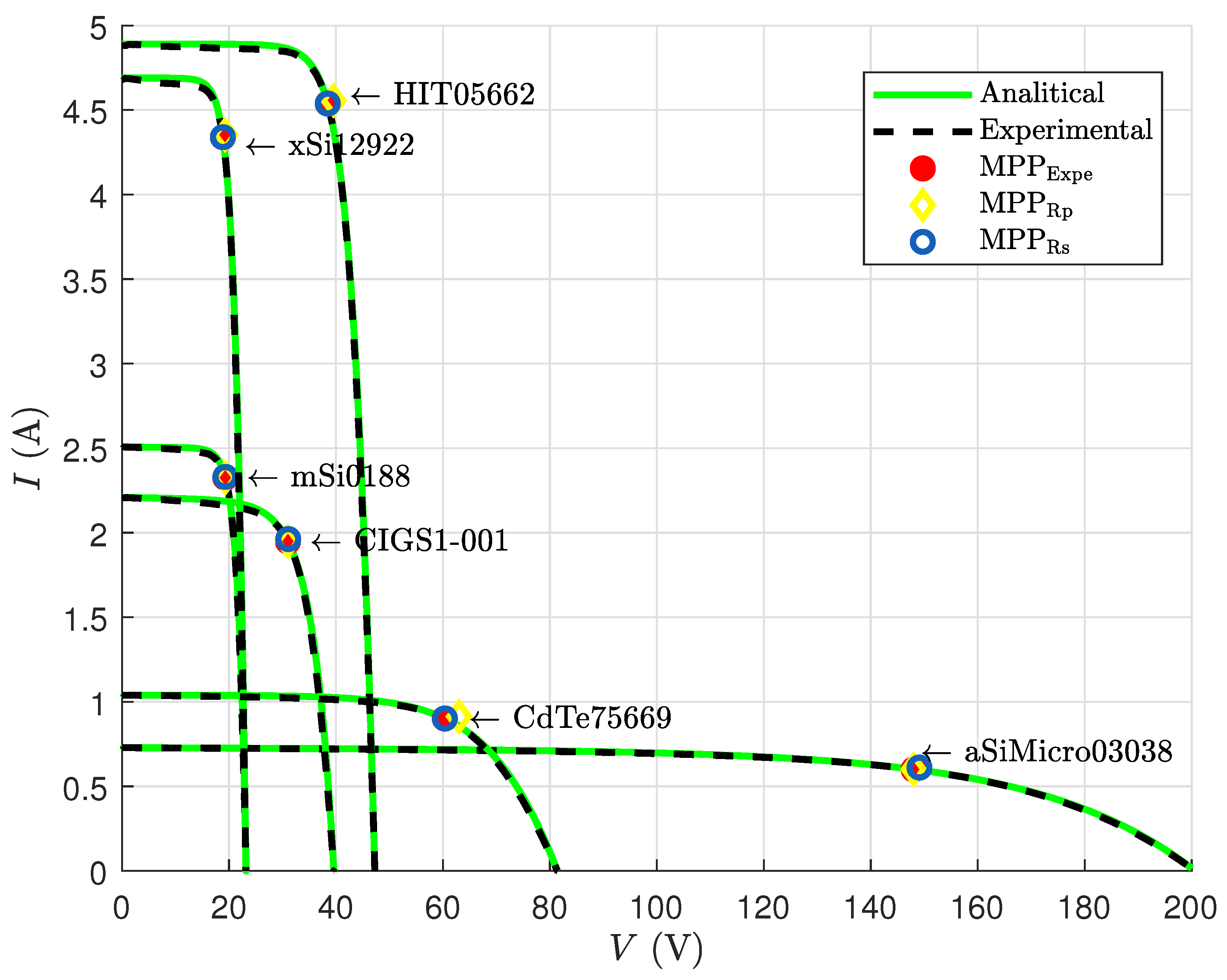
summarizes the PV metrics and the simplified SDM parameters for the six studied PV technologies. The characteristic parameters were calculated using the explicit solutions presented in [24,25]. Figure 1 shows the IV curve and MPP for each module and analytical method. Figure 2 displays the base-10 logarithm of the relative error (in %) between the experimental measurements and the simplified SDM model of the current with respect to the normalized voltage. It can be observed that the error is small around the extremes of the curve ($V_{\mathrm{oc}}$ and $I_{\mathrm{sc}}$) and in the MPP. This is because the methodology seeks to match the experimental curve IV with the theoretical curve at these points. This is sufficient for the methodology presented in this work, which seeks to obtain the highest accuracy in the vicinity of the MPP.

Table 3. APE (%) between the analytical approximations and experimental measurements of $V_{\mathrm{mpp}}$ and $I_{\mathrm{mpp}}$.

Model	Proposed Model		Tirado		Batzelis		Wang		Numerical
	${\mathit{V}}_{\mathbf{mpp}}$	${\mathit{I}}_{\mathbf{mpp}}$	${\mathit{V}}_{\mathbf{mpp}}$	${\mathit{I}}_{\mathbf{mpp}}$	${\mathit{V}}_{\mathbf{mpp}}$	${\mathit{I}}_{\mathbf{mpp}}$	${\mathit{V}}_{\mathbf{mpp}}$	${\mathit{I}}_{\mathbf{mpp}}$	${\mathit{V}}_{\mathbf{mpp}}$	${\mathit{I}}_{\mathbf{mpp}}$
aSiMicro03036	$2.03\times {10}^{-7}$	$2.02\times {10}^{-7}$	$8.65\times {10}^{-1}$	$7.76\times {10}^{-1}$	$7.27\times {10}^{-1}$	$7.40\times {10}^{-1}$	$6.01\times {10}^{-1}$	$7.01\times {10}^{-1}$	$1.88\times {10}^{-7}$	$2.17\times {10}^{-7}$
mSi0188	$7.31\times {10}^{-6}$	$4.74\times {10}^{-6}$	$1.23\times {10}^{-1}$	$1.23\times {10}^{-1}$	$3.18\times {10}^{-2}$	$3.19\times {10}^{-2}$	$1.40\times {10}^0$	$1.53\times {10}^0$	$7.31\times {10}^{-6}$	$4.74\times {10}^{-6}$
CIGS1-001	$3.36\times {10}^{-6}$	$2.92\times {10}^{-6}$	$3.74\times {10}^{-1}$	$3.75\times {10}^{-1}$	$1.79\times {10}^{-1}$	$1.80\times {10}^{-1}$	$1.96\times {10}^0$	$2.12\times {10}^0$	$3.36\times {10}^{-6}$	$2.92\times {10}^{-6}$
xSi12922	$2.63\times {10}^{-3}$	$1.71\times {10}^{-3}$	$1.71\times {10}^{-1}$	$1.73\times {10}^{-1}$	$3.30\times {10}^{-1}$	$3.23\times {10}^{-1}$	$1.11\times {10}^0$	$1.19\times {10}^0$	$2.63\times {10}^{-3}$	$1.71\times {10}^{-3}$
CdTe75669	$3.47\times {10}^{-2}$	$3.21\times {10}^{-2}$	$8.12\times {10}^{-1}$	$8.22\times {10}^{-1}$	$1.32\times {10}^0$	$1.27\times {10}^0$	$1.20\times {10}^{-1}$	$1.10\times {10}^{-1}$	$3.47\times {10}^{-2}$	$3.21\times {10}^{-2}$
HIT05662	$5.11\times {10}^{-3}$	$3.36\times {10}^{-3}$	$1.67\times {10}^{-1}$	$1.68\times {10}^{-1}$	$4.17\times {10}^{-1}$	$4.06\times {10}^{-1}$	$8.76\times {10}^{-1}$	$9.25\times {10}^{-1}$	$5.11\times {10}^{-3}$	$3.36\times {10}^{-3}$
MAPE	$7.08\times {10}^{-3}$	$6.20\times {10}^{-3}$	$4.18\times {10}^{-1}$	$4.06\times {10}^{-1}$	$5.01\times {10}^{-1}$	$4.91\times {10}^{-1}$	$1.01\times {10}^0$	$1.10\times {10}^0$	$7.08\times {10}^{-3}$	$6.20\times {10}^{-3}$

shows the absolute percentage error (APE) between the calculated and the measured $V_{\mathrm{mpp}}$, $I_{\mathrm{mpp}}$. The APE is provided by

$$\mathrm{APE}=\frac{\left|X-X_{\exp }\right|}{X_{\exp }}\times 100(\%),$$

(66)

where $X_{\exp }$ represents the experimental measurements of the MPP and X represents calculation of the MPP for each technology using the presented methodology. In addition, three well-established methods from the literature are used to make comparisons, labeled “Batzelis” for the method presented in [35], “Wang” for [20], and “Tirado” for [21]. For the numerical solutions, these are obtained for the implicit Equations (27) and (47) using Matlab’s built-in fzero solver with Equations (35) and (49) as the respective initial values. According to the methodology used to calculate the SDM parameters, the expressions presented in the Section 4 are use for the modules “xSi12922”, “CdTe75669”, and “HIT05662”, while the expressions presented in Section 5 are used for the other three modules.

Of the three methods used for comparison, the one presented in [21] performs best in estimating the MPP of the xSi12922 and HIT05662 technologies, the method presented in [20] performs best for the aSiMicro and CdTe modules, and the method presented in [35] performs best for the CIGS and mSi0188 technologies. However, the smallest mean of APE for the six modules is achieved by the method from [21], with 0.418% and 0.406% for $V_{\mathrm{mpp}}$ and $I_{\mathrm{mpp}}$, respectively, followed by [35] with 0.501% and 0.491%. The method with the largest mean APE is [20], with 1.011% for $V_{\mathrm{mpp}}$ and 1.096% for $I_{\mathrm{mpp}}$. The best performance is obtained by the numerical solution and the method proposed in this work, both with similar accuracy of 7.077 $\times {10}^{-3}$% for $V_{\mathrm{mpp}}$ and 6.195 $\times {10}^{-3}$% for $I_{\mathrm{mpp}}$, showing superior performance compared to the previously published methods. The reason for this is that the previous methods depend on the values of both resistors (series and shunt); thus, if one is neglected, the resulting expression is strongly affected and becomes significantly inaccurate.

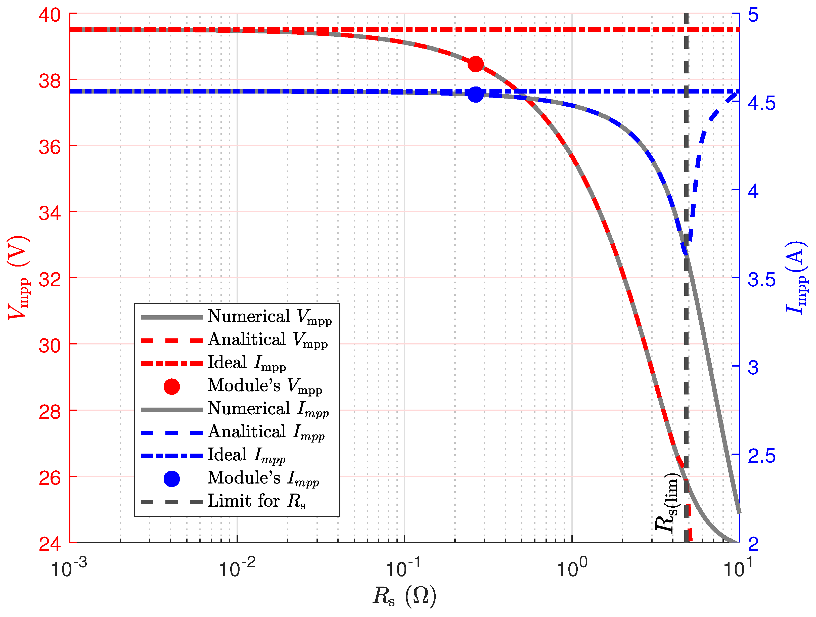
Figure 3 and Figure 4 display the curves of $V_{\mathrm{mpp}}$ and $I_{\mathrm{mpp}}$ with respect to $R_{\mathrm{p}}$ and $R_{\mathrm{s}}$ (with the scale axis in base-10 logarithm) for the aSiMicro03036 and HIT05662 technologies, respectively. Here, the first five terms of Equations (59) and (42) are compared to the numerical approximation using Equations (47) and (27). The MPP value of the module is marked with a dot, while the limits for $R_{\mathrm{p}}$ (from Equation (65)) and $R_{\mathrm{s}}$ (from Equation (33)) are indicated with a vertical dashed line. In Figure 3, it can be observed that there is a good fit between the analytical and numerical approximation for values of $R_{\mathrm{p}}>R_{\mathrm{p}}\left(\lim \right)$, and $V_{\mathrm{mpp}}$ tends to the ideal case as $R_{\mathrm{p}}$ continues to increase. On the other hand, the series diverges for values $R_{\mathrm{p}}<R_{\mathrm{p}}\left(\lim \right)$; however, the range covered by $rpl$ is sufficient to satisfy practical cases. From Figure 4, it can be seen that the values calculated with the new analytical model are in good agreement with the numerical reference model for $R_{\mathrm{s}}<R_{\mathrm{s}}\left(\lim \right)$. For $R_{\mathrm{s}}>R_{\mathrm{s}}\left(\lim \right)$, the value of $V_{\mathrm{mpp}}$ calculated with Eqution (42) appears to decrease, while $I_{\mathrm{mpp}}$ increases with increasing $R_{\mathrm{s}}$, showing a clear divergence of the power series.

Figure 5 and Figure 6 compare the APE for the numerical and the analytical solutions as a function of $R_{\mathrm{p}}$ and $R_{\mathrm{s}}$ for the aSiMicro03036 and HIT05662 technologies and for different numbers of terms in the power-series of Equations (59) and (42). In Figure 6, it can be observed that the APE increases as $R_{\mathrm{p}}$ decreases; taking one term of Equation (42), the approximation yields an APE of 25.98% for $V_{\mathrm{mpp}}$ and 28.51% for $I_{\mathrm{mpp}}$ at $R_{\mathrm{p}}=R_{\mathrm{p}}\left(\lim \right)=298.19\mathrm{\Omega }$. Increasing $R_{\mathrm{p}}$ up to the modulus value $R_{\mathrm{p}}=9532\mathrm{\Omega }$ provides an APE of 1.51 $\times {10}^{-2}$% for both $V_{\mathrm{mpp}}$ and $I_{\mathrm{mpp}}$, while in the limiting case $R_{\mathrm{p}}=1\times {10}^5\mathrm{\Omega }$ the APE is equal to 1.36 $\times {10}^{-6}$%. The APE decreases significantly when increasing the number of terms; estimating the performance for $R_{\mathrm{p}}=R_{\mathrm{p}}\left(\lim \right)=298.19$ $\mathrm{\Omega }$, an $APE$ of 0.719% is calculated by taking five terms, significantly improving the accuracy in this extreme case. Figure 5 shows that the APE increases as $R_{\mathrm{s}}$ increases; this is because the approximation provided by Equation (42) performs better as $R_{\mathrm{s}}$ decreases. It is also observed that in the vicinity of $R_{\mathrm{s}}=R_{\mathrm{s}}\left(\lim \right)$, the APE decreases rapidly as $R_{\mathrm{s}}$ decreases, from an $APE=20.127$% for one term down to $APE=0.295$% using five terms. For the case where $R_{\mathrm{s}}=0.2656$ $\mathrm{\Omega }$, the APE ranges from 1.4148 $\times {10}^{-4}$% for one term to 3.9139 $\times {10}^{-14}$% for five terms, showing significantly improved accuracy of the approximation. Thus, if computational resources are limited, as is the case with real-time MPP estimation using low-cost hardware, it is possible to take the first terms of the series. If requirements are less stringent, it is possible to take as many terms as the level of accuracy requires.

A limitation of the methodology presented here is that it depends on the existence of a small parameter in the equations, introduced in the formulations presented in this work as $\eta$ (provided by (39)) and $\phi$ (provided by (55)). Furthermore, the convergence of the power series depends strongly on how small these parameters are. However, using a large amount of data, we found that the values of these parameters fell within the established limits.

7. Conclusions

In this paper, we have derived formulas for calculating the maximum power point that can explicitly take into account the separate effects of series and shunt resistance. We have found approximations of the transcendental equations for MPP calculation in terms of simplified SDM parameters by employing perturbation theory and the Lagrange inversion theorem. These expressions were validated using the calculated and measured IV curves of six PV modules based on different technologies. The verification results reveal that the APE between the presented approximations and the experimental measurements is less than 0.035%, which is useful in most engineering applications. The formulas can be simplified or made more complex depending on the computational cost and accuracy needs of the specific application. In the future, we intend to extend the presented models to five-parameter SDM using the methods developed in this work.