Proposal of Low-Speed Sensorless Control of IPMSM Using a Two-Interval Six-Segment High-Frequency Injection Method with DC-Link Current Sensing

Abstract

This paper proposes a modification to existing saliency-based, sensorless control strategy for interior permanent magnet synchronous motors. The proposed approach leverages a two-interval, six-segment high-frequency voltage signal injection technique. It aims to improve rotor position and speed estimation accuracy when utilizing a single current sensor positioned in the inverter’s DC-bus circuit. The key innovation lies in modifying both the high-frequency signal injection and demodulation processes to address challenges in accurate phase current reconstruction and rotor position estimation, at low and zero speeds. A significant modification to the traditional high-frequency voltage signal injection method is introduced, which involves splitting the signal injection and the field-oriented control algorithm into two distinct sampling and switching periods. This approach ensures that no portion of the injected voltage space vector falls into the immeasurable region of space vector modulation, which could otherwise compromise current measurements. The dual-period structure, termed the two-interval six-segment high-frequency injection, allows for more precise current measurement during the signal injection period while maintaining optimal motor control during the field-oriented control period. Furthermore, this paper explores a different demodulation technique that improves the estimation of rotor position and speed. By employing a synchronous filter in combination with a phase-locked loop, the proposed method enhances the robustness of the system against noise and inaccuracies typically encountered in phase current reconstruction. The effectiveness of the proposed modifications is demonstrated through comprehensive simulation results. These results confirm that the enhanced method offers more reliable rotor position and speed estimates compared to the existing sensorless technique, making it particularly suitable for applications requiring high precision in motor control.

1. Introduction

The control of interior permanent magnet synchronous motors (IPMSMs) is critical in applications requiring high performance, such as electric vehicles and industrial automation. However, traditional control methods often rely on position sensors, which can add cost and complexity to the system. Sensorless control techniques have emerged as a viable alternative, particularly in environments where sensor reliability is compromised or where reducing system complexity is essential.

Among sensorless techniques, saliency-based methods, which exploit the inherent anisotropies of the motor, have gained considerable attention. These methods are particularly effective at low speeds and during standstill, where back-EMF-based methods falter [1,2,3,4]. However, existing saliency-based techniques face challenges in accurately estimating rotor position and speed due to issues such as noise and inaccuracies in phase current reconstruction [5,6,7,8,9,10].

This paper proposes a modification to an advanced saliency-based sensorless control method initially published by Zhao et al. [11]. The original method is based on the sinusoidal injection of a high-frequency (HF) signal in a stationary reference frame. However, it may encounter challenges related to the accurate reconstruction of phase currents within the immeasurable areas of space vector modulation (SVM). The modification proposed in this paper aims to overcome these challenges. We introduce a two-interval, six-segment high-frequency injection approach that incorporates a modified current reconstruction scheme, as designed by Zhao et al. to enhance the accuracy of the reconstructed current. Additionally, we propose an alternative demodulation technique in combination with the saliency-based sensorless control method to address key challenges in rotor position and speed estimation for IPMSMs. This approach utilizes a synchronous filter and a phase-locked loop (PLL) to further improve the precision of rotor position and speed estimation. This paper details the mathematical foundation, implementation, and results of extensive simulations, validating the effectiveness of the proposed methods.

This article is organized as follows: Section 2 introduces the mathematical model of the IPMSM relevant to the HF injection method and outlines the separation of HF components using the band-pass filter (BPF). Then, it presents the HF injection method adopted for the purposes of this article in Section 2.1. Section 2.2 describes the demodulation process. Section 2.3 outlines the phase current reconstruction scheme and a potential problem with the adopted HF injection method in combination with that scheme and proposes a solution. In Section 3, simulation results are presented to validate the effectiveness of the proposed control strategy. Finally, Section 4 concludes this paper by summarizing the key findings.

2. Proposed Saliency-Based Sensorless Control Method

Since this article addresses saliency-based sensorless methods, it is necessary to introduce a mathematical model of the examined IPMSM. Because these methods rely on the injection of HF signals, an appropriate form of the mathematical model is required. The mathematical model in the $\alpha \beta$ stationary reference frame is employed. At high frequencies, the derivative terms with inductance dominate the voltage equations in the standard dynamic model of the IPMSM. Therefore, terms involving stator resistance can be neglected, as well as induced voltage, as saliency-based sensorless methods are utilized at zero and low speeds.

The voltage equations can then be divided into two parts: one that rotates with the electrical angular velocity and the other representing the HF part. A BPF is introduced to separate the HF part from the component including the basic current harmonic. After filtering, the voltage equations take the form given in (1).

$$\left(\begin{array}{c}{V}_{\alpha \mathrm{h}\mathrm{f}}\\ V_{\beta \mathrm{h}\mathrm{f}}\end{array}\right)={\mathbf{L}}_{\alpha \beta }{\displaystyle \frac{d}{dt}}\left(\begin{array}{c}{i}_{\alpha \mathrm{h}\mathrm{f}}\\ i_{\beta \mathrm{h}\mathrm{f}}\end{array}\right),$$

(1)

where $V_{x\mathrm{h}\mathrm{f}}$ are components of the HF injection voltage and $i_{x\mathrm{h}\mathrm{f}}$ are components of the HF stator current response, both in the $\alpha \beta$ reference frame. ${\mathbf{L}}_{\alpha \beta }$ represents the inductance matrix and is described as follows:

$${\mathbf{L}}_{\alpha \beta }=\left(\begin{array}{cc}{L}_0+L_{\Delta }cos\left(2{\theta }_e\right)& L_{\Delta }sin\left(2{\theta }_e\right)\\ L_{\Delta }sin\left({\theta }_e\right)& L_0-L_{\Delta }cos\left(2{\theta }_e\right)\end{array}\right),$$

(2)

where $L_0={\displaystyle \frac{L_d+L_q}{2}}$ and $L_{\Delta }={\displaystyle \frac{L_d-L_q}{2}}$. ${\theta }_e$ represents electrical rotor position. The second harmonic of the rotor saliency is observable in the inductance matrix and is utilized for rotor speed and position estimation. To accomplish this, it is crucial to first compute the HF stator current response. Therefore, Equation (1) has to be manipulated as seen in (3) and integrated afterwards.

$${\displaystyle \frac{d}{dt}}\left(\begin{array}{c}{i}_{\alpha \mathrm{h}\mathrm{f}}\\ i_{\beta \mathrm{h}\mathrm{f}}\end{array}\right)={\mathbf{L}}_{\alpha \beta }^{-1}\left(\begin{array}{c}{V}_{\alpha \mathrm{h}\mathrm{f}}\\ V_{\beta \mathrm{h}\mathrm{f}}\end{array}\right),$$

(3)

where ${\mathbf{L}}_{\alpha \beta }^{-1}$ is described as follows:

$${\mathbf{L}}_{\alpha \beta }^{-1}={\displaystyle \frac{1}{L_d{L}_q}}\left(\begin{array}{cc}{L}_0-L_{\Delta }cos\left(2{\theta }_e\right)& -L_{\Delta }sin\left(2{\theta }_e\right)\\ -L_{\Delta }sin\left(2{\theta }_e\right)& L_0+L_{\Delta }cos\left(2{\theta }_e\right)\end{array}\right).$$

(4)

The mentioned BPF should be set so that its bandwidth is centered around the difference between twice the basic current harmonic frequency and the frequency of the HF current response, as shown in (7). This assumption is further supported by a Fourier analysis. Figure 1 illustrates such an analysis of the reconstructed phase current with the HF injection described further below. With a sampling frequency of $f_{\mathrm{s}}=25\mathrm{kHz}$, the injection frequency is $f_{\mathrm{hf}}={\displaystyle \frac{f_{\mathrm{s}}}{6}}\approx 4.17\mathrm{kHz}$, which corresponds with the results.

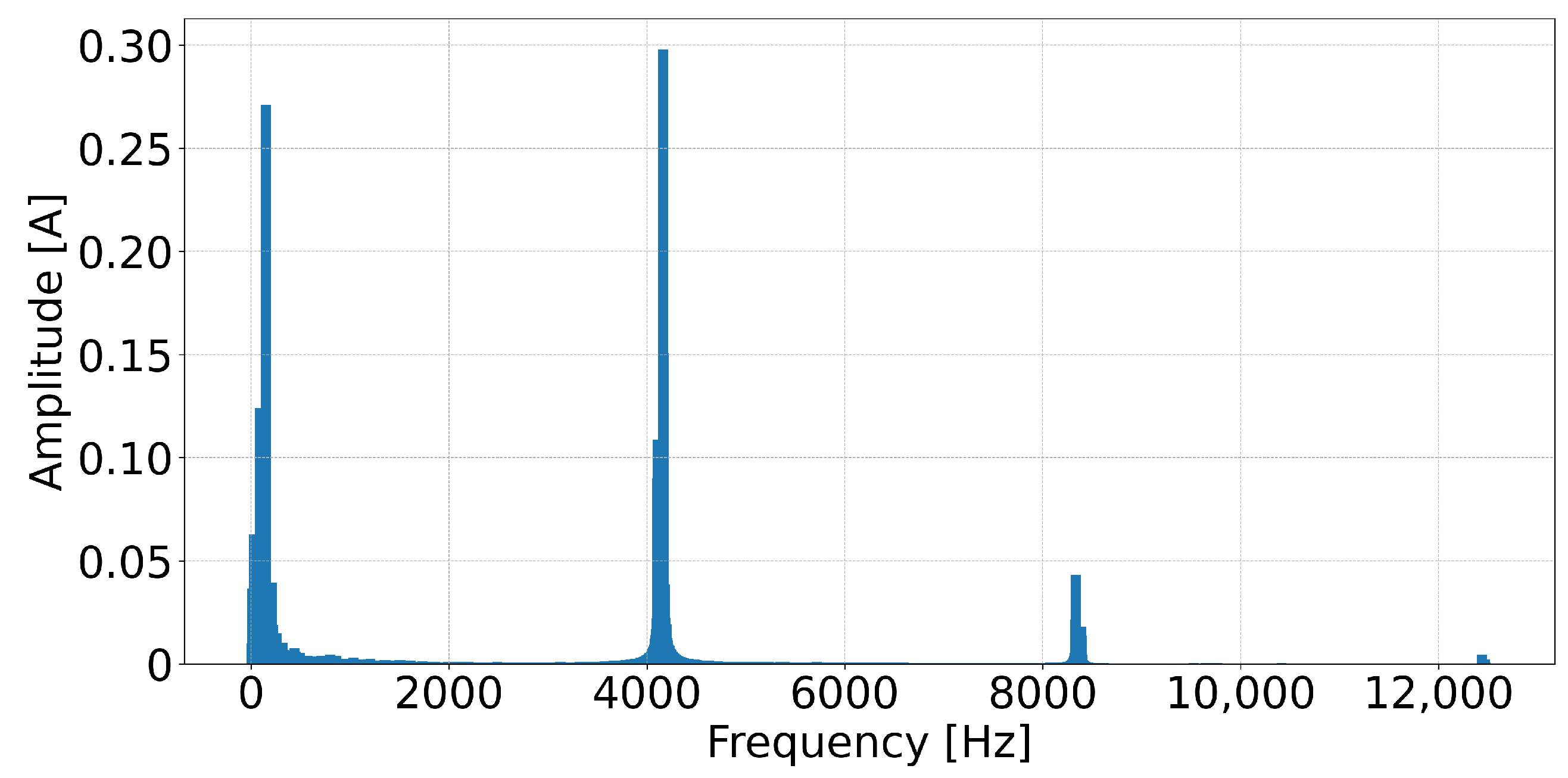
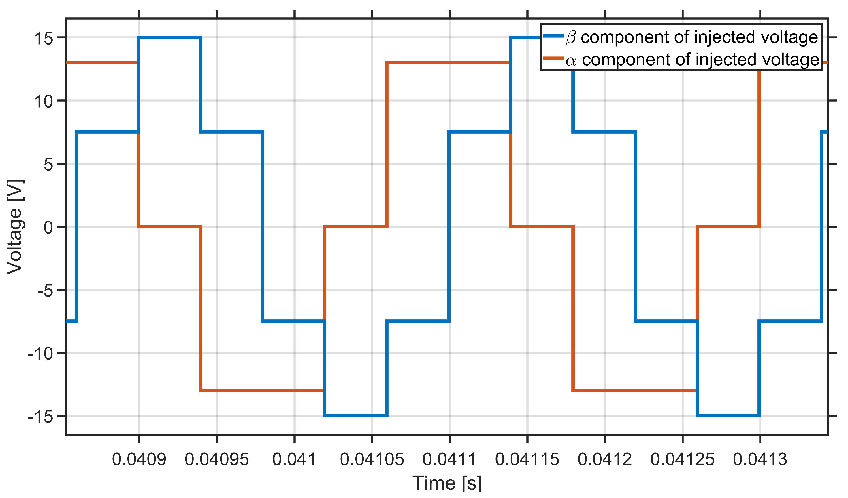
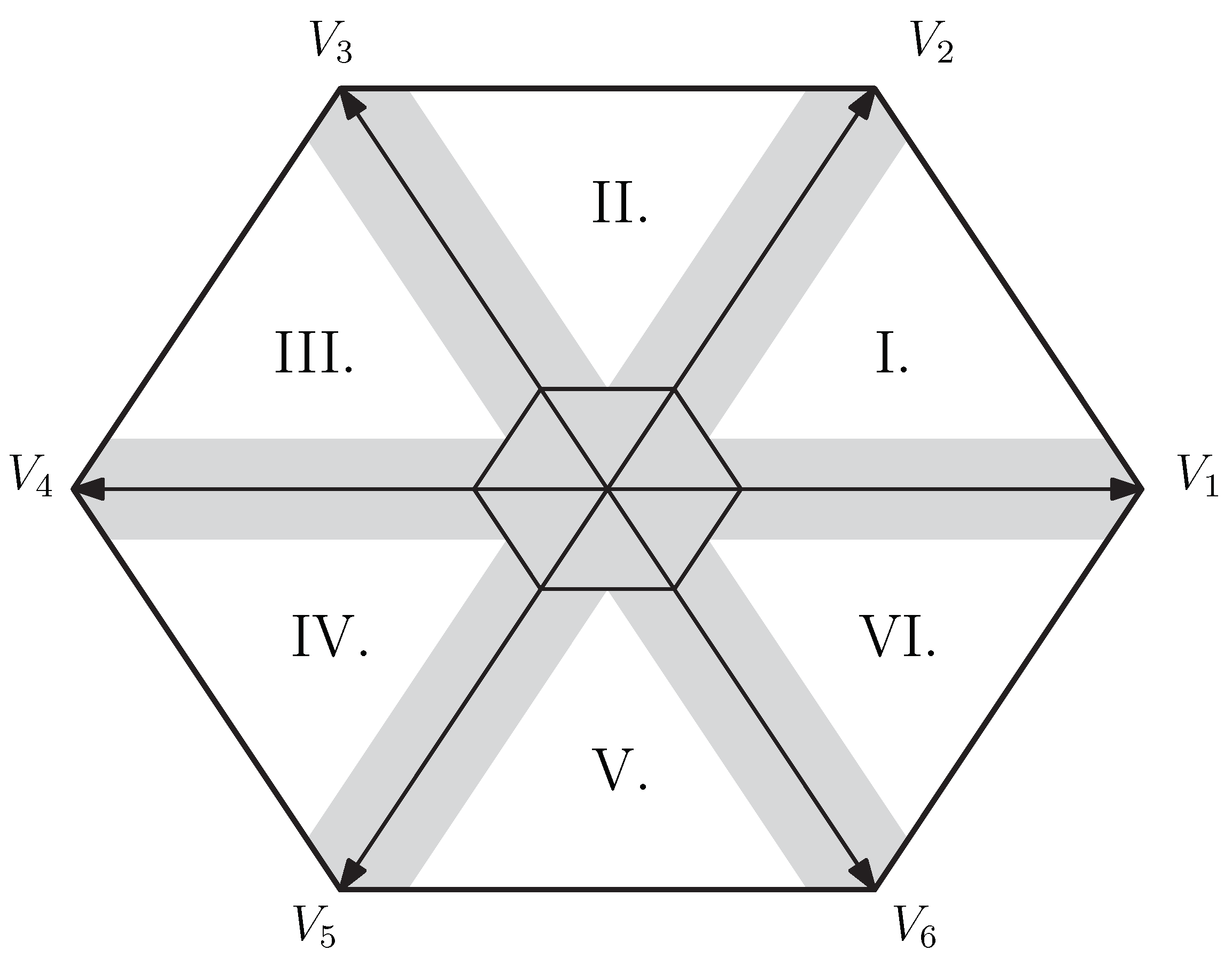
2.1. Six-Segment High-Frequency Injection Method

An injection method, proposed by Zhao et al. [11] and adopted with necessary modifications for the purposes of this article, rotates a voltage space vector successively through each sector. This injection method can be regarded as a HF sinusoidal injection, described by (5), where the angular velocity of the injected voltage is given by ${\omega }_{\mathrm{hf}}={\displaystyle \frac{2\pi }{6}}{f}_{\mathrm{s}}$, with $f_{\mathrm{s}}$ being the sampling frequency. The mentioned modifications will be further described in Section 2.3.

$$\left(\begin{array}{c}{V}_{\alpha \mathrm{h}\mathrm{f}}\\ V_{\beta \mathrm{h}\mathrm{f}}\end{array}\right)=V_{\mathrm{hf}}\left(\begin{array}{c}cos\left({\omega }_{\mathrm{hf}}t\right)\\ sin\left({\omega }_{\mathrm{hf}}t\right)\end{array}\right)$$

(5)

The waveform represented by (5) is shown in Figure 2. The amplitude of the injected voltage $V_{\mathrm{hf}}$ was set to $15\mathrm{V}$. The reason for choosing this value will be explained below in Section 2.3.

By substituting (5) and (4) into (3) and integrating, (6) is obtained. After simplification, the equation describing the HF current response in stationary $\alpha \beta$ can be written as (7).

$$\left(\begin{array}{c}{i}_{\alpha \mathrm{h}\mathrm{f}}\\ i_{\beta \mathrm{h}\mathrm{f}}\end{array}\right)={\displaystyle \frac{1}{L_d{L}_q}}\left(\begin{array}{cc}{L}_0-L_{\Delta }cos\left(2{\theta }_e\right)& -L_{\Delta }sin\left(2{\theta }_e\right)\\ -L_{\Delta }sin\left(2{\theta }_e\right)& L_0+L_{\Delta }cos\left(2{\theta }_e\right)\end{array}\right)\int \left(\begin{array}{c}cos\left({\omega }_{\mathrm{hf}}t\right)\\ sin\left({\omega }_{\mathrm{hf}}t\right)\end{array}\right)$$

(6)

$$\left(\begin{array}{c}{i}_{\alpha \mathrm{h}\mathrm{f}}\\ i_{\beta \mathrm{h}\mathrm{f}}\end{array}\right)={\displaystyle \frac{V_{\mathrm{hf}}}{L_d{L}_q{\omega }_{\mathrm{hf}}}}\left(\begin{array}{c}{L}_{\Delta }sin\left(2{\theta }_e-{\theta }_{\mathrm{hf}}\right)+L_{0}sin\left({\theta }_{\mathrm{hf}}\right)\\ -L_{\Delta }cos\left(2{\theta }_e-{\theta }_{\mathrm{hf}}\right)-L_{0}cos\left({\theta }_{\mathrm{hf}}\right)\end{array}\right)$$

(7)

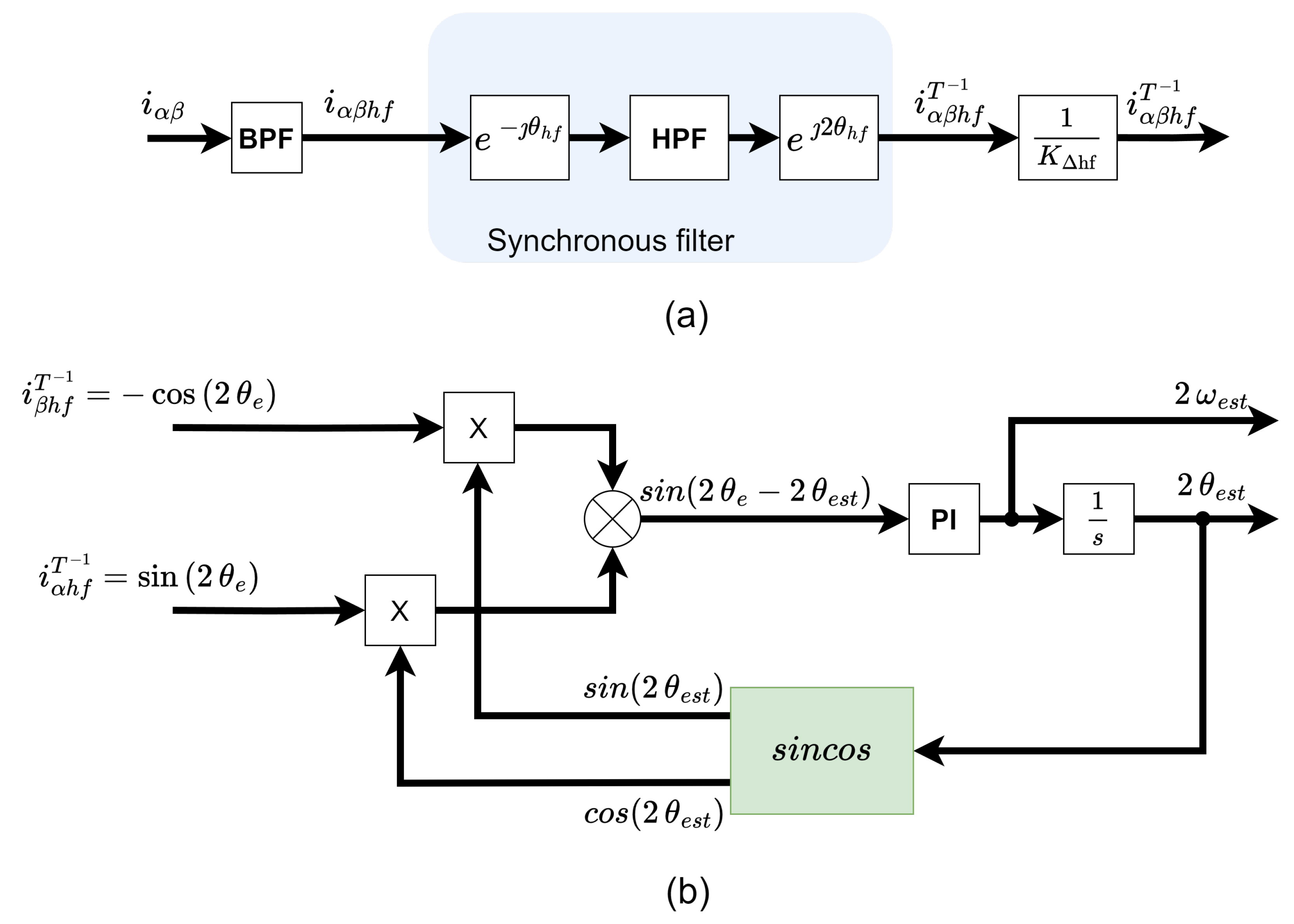
2.2. Demodulation of HF Current Response

The proposed high-frequency demodulation approach here, a method to extract information about rotor speed and position, differs from the one proposed by Zhao et al. [11]. The different approach to high-frequency current response demodulation is one of two key innovations presented in this article.

The proposition is to employ the so-called synchronous filter. The rationale behind using this demodulation technique is that, by employing multiple filters to isolate only the relevant frequencies from the current response signals across different reference frames, the method is expected to be less susceptible to phase current reconstruction errors. Consequently, we anticipate smaller deviations in the estimated position during steady-state operation compared to other methods.

The principle of operation lies in using the Park transformation into a synchronous reference frame rotating with the angular velocity of the injected signal ${\omega }_{\mathrm{hf}}$, as shown in (8) and, after simplification, in (9). ${\theta }_{\mathrm{hf}}$ represents the position of the space vector of the injected signal.

$${\left(\begin{array}{c}{i}_{\alpha \mathrm{h}\mathrm{f}}\\ i_{\beta \mathrm{h}\mathrm{f}}\end{array}\right)}^{\mathrm{T}}=\left(\begin{array}{cc}cos\left({\theta }_{\mathrm{hf}}\right)& sin\left({\theta }_{\mathrm{hf}}\right)\\ -sin\left({\theta }_{\mathrm{hf}}\right)& cos\left({\theta }_{\mathrm{hf}}\right)\end{array}\right)\left(\begin{array}{c}{i}_{\alpha \mathrm{h}\mathrm{f}}\\ i_{\beta \mathrm{h}\mathrm{f}}\end{array}\right)$$

(8)

$${\left(\begin{array}{c}{i}_{\alpha \mathrm{h}\mathrm{f}}\\ i_{\beta \mathrm{h}\mathrm{f}}\end{array}\right)}^{\mathrm{T}}={\displaystyle \frac{V_{\mathrm{hf}}}{L_d{L}_q{\omega }_{\mathrm{hf}}}}\left(\begin{array}{c}{L}_{\Delta }sin\left(2{\theta }_e-2{\theta }_{\mathrm{hf}}\right)\\ -L_0-L_{\Delta }cos\left(2{\theta }_e-2{\theta }_{\mathrm{hf}}\right)\end{array}\right)$$

(9)

Then, a high-pass filter (HPF) is introduced to separate the useful part of the signal from the DC component, as described by (10), with a substitution given in (11).

$${\left(\begin{array}{c}{i}_{\alpha \mathrm{h}\mathrm{f}}\\ i_{\beta \mathrm{h}\mathrm{f}}\end{array}\right)}_{\mathrm{HPF}}^{\mathrm{T}}=K_{\Delta \mathrm{h}\mathrm{f}}\left(\begin{array}{c}sin\left(2{\theta }_e-2{\theta }_{\mathrm{hf}}\right)\\ -cos\left(2{\theta }_e-2{\theta }_{\mathrm{hf}}\right)\end{array}\right)$$

(10)

$$K_{\Delta \mathrm{h}\mathrm{f}}={\displaystyle \frac{V_{\mathrm{hf}}{L}_{\Delta }}{L_d{L}_q{\omega }_{\mathrm{hf}}}}$$

(11)

Now, another Park transformation is used. From (10), it is apparent that the HF current response contains two sine and cosine components, respectively. The first component is associated with the electrical position, while the second component is related to the position of the HF injected signal, which rotates in the opposite direction. To eliminate the second component, the inverse-Park transformation is applied to convert the signals into a synchronous reference frame rotating at twice the angular velocity of the injected signal, as described in (12) and, after simplification, in (13).

$${\left(\begin{array}{c}{i}_{\alpha \mathrm{h}\mathrm{f}}\\ i_{\beta \mathrm{h}\mathrm{f}}\end{array}\right)}^{{\mathrm{T}}^{-1}}=\left(\begin{array}{cc}cos\left(2{\theta }_{\mathrm{hf}}\right)& -sin\left(2{\theta }_{\mathrm{hf}}\right)\\ sin\left(2{\theta }_{\mathrm{hf}}\right)& cos\left(2{\theta }_{\mathrm{hf}}\right)\end{array}\right){\left(\begin{array}{c}{i}_{\alpha \mathrm{h}\mathrm{f}}\\ i_{\beta \mathrm{h}\mathrm{f}}\end{array}\right)}_{\mathrm{HPF}}^{\mathrm{T}}$$

(12)

From (13), it is apparent that the employed synchronous filter has removed the HF component. The $\alpha \beta$ signal at the output of the filter consists of sine and cosine functions, each with an argument of twice the electrical position, and an amplitude given by (11).

$${\left(\begin{array}{c}{i}_{\alpha \mathrm{h}\mathrm{f}}\\ i_{\beta \mathrm{h}\mathrm{f}}\end{array}\right)}^{{\mathrm{T}}^{-1}}=K_{\Delta \mathrm{h}\mathrm{f}}\left(\begin{array}{c}sin\left(2{\theta }_e\right)\\ -cos\left(2{\theta }_e\right)\end{array}\right)$$

(13)

To extract the position information, a PLL structure is employed. The output of the PLL is the estimated position ${\theta }_{\mathrm{est}}$. The input value for the PLL is the error ${\theta }_{\mathrm{est}.\mathrm{error}}$ between the electrical position ${\theta }_e$ and the estimated position ${\theta }_{\mathrm{est}}$, given by ${\theta }_{\mathrm{est}.\mathrm{error}}={\theta }_e-{\theta }_{\mathrm{est}}$. The PLL’s task is to drive this error ${\theta }_{\mathrm{est}.\mathrm{error}}$ to zero. Since $sin\left(x\right)\approx 0$ when $x\to 0$, the trigonometric formula for $sin\left(x-y\right)$ shown in (14) can be used instead.

$$sin(x-y)=sin\left(x\right)cos\left(y\right)-cos\left(x\right)sin\left(y\right)$$

(14)

After substituting the appropriate terms from (13), along with the sine and cosine functions of ${\theta }_{\mathit{est}}$, into (14), the resulting equations are expressed as (15) and (16).

$$\begin{array}{cc}\hfill sin\left(2{\theta }_e-2{\theta }_{\mathit{est}}\right)& ={\displaystyle \frac{i_{\alpha hf}^{T^{-1}}}{K_{\Delta \mathrm{h}\mathrm{f}}}}cos\left(2{\theta }_{\mathit{est}}\right)+{\displaystyle \frac{i_{\beta hf}^{T^{-1}}}{K_{\Delta \mathrm{h}\mathrm{f}}}}sin\left(2{\theta }_{est}\right)=\hfill \end{array}$$

(15)

$$\begin{array}{cc}\hfill & =sin\left(2{\theta }_e\right)cos\left(2{\theta }_{est}\right)-cos\left(2{\theta }_e\right)sin\left(2{\theta }_{est}\right)\hfill \end{array}$$

(16)

Figure 3 then illustrates the block diagram of the synchronous filter with the PLL.

2.3. Two-Interval Six-Segment HF Injection

Authors Zhao et al. [11] also proposed a modified three-phase current reconstruction scheme, which employed all active vectors in any given pulse-width modulation (PWM) period to measure four DC-link currents corresponding to two different phase currents and use them all to reconstruct three-phase currents. The purpose of this scheme is to overcome the effect of unaligned (asynchronous) sample timing in the traditional phase current reconstruction scheme, where only two samples per period are taken. The core of this scheme lies in the calculation of the average values of phase currents from two DC-link samples corresponding to the same phase current taken at different instants in one given PWM period. Figure 4 shows the simulation verification of this modified current reconstruction scheme. A detailed view of a phase current as measured directly (yellow), a phase current reconstructed using a standard scheme (red), and a phase current reconstructed using modified scheme (blue), are portrayed.

It is apparent that, compared to the traditional reconstruction scheme, it demonstrates better reconstruction accuracy. For more details, please see the original article by Zhao et al. [11].

Furthermore, Figure 5 shows the Fourier analysis of phase current reconstruction using the modified current reconstruction scheme. It can be observed that, compared to Figure 1, which presents the Fourier analysis of phase current reconstruction using the standard current reconstruction scheme, the modified scheme exhibits fewer higher harmonics in the signal. This reduction is significant for the demodulation process.

Therefore, the modified current reconstruction scheme is adopted for the purposes of this article.

2.3.1. Problem Statement

In combination with their proposed six-segment injection method, authors Zhao et al. [11] state that it is not necessary to employ any PWM pattern modifications to ensure a sufficient DC-link current sampling window. Active vector pulse widths created by the injected voltage space vectors (depending on the injected voltage amplitude) are sufficient to sample each DC-link current corresponding to two different phase currents. In other words, the voltage space vector is never in the immeasurable area, as shown in Figure 6.

Since authors Zhao et al. [11] propose to superimpose the injected voltage space vector and the reference voltage space vector, a situation may occur where this superposition creates a resulting space vector inside the immeasurable area. For example, if the injected voltage space vector is in sector I. and the reference voltage space vector is in sector III., the resulting space vector can reach the immeasurable area, provided that the amplitude of the reference voltage space vector is large enough.

2.3.2. Proposed Solution

To overcome this limitation, another modification is proposed in this article. First, assume the following:

• The field-oriented control (FOC) structure is implemented and calculated every sampling period after samples of current, voltage, and other useful or mandatory quantities are taken.
• The sampling frequency $f_{\mathrm{s}}$ is equal to the switching frequency $f_{\mathrm{sw}}$.
• The DC-link current sensor is placed in the bottom current path between the DC-bus and the individual phases.

Under these assumptions, the sampling period can be divided into two types. In the first, termed the FOC period, the FOC structure will be calculated and the reconstruction of three-phase currents will be performed. In the second, termed the INJ period, the HF voltage injection and demodulation occur. The sampling frequency $f_{\mathrm{s}}$ will remain the same as the switching frequency $f_{\mathrm{sw}}$, but the FOC and INJ periods will alternate, meaning that each one will have an execution frequency of half the switching or sampling frequency, $f_{\mathrm{control}}={\displaystyle \frac{1}{2}}{f}_{\mathrm{sw}}={\displaystyle \frac{1}{2}}{f}_{\mathrm{s}}$. This division into FOC and INJ periods gives rise to the term “two-interval” six-segment HF injection. Figure 7 illustrates this scheme with a timing diagram for the PWM module in conjunction with the analog-to-digital converter (ADC).

This approach ensures that there is no situation where any of the active vectors would be insufficiently wide for measuring the DC-link current and subsequent reconstruction of phase currents, given that the injection space vectors are outside the immeasurable area. This is why the amplitude of the injected voltage $V_{\mathrm{hf}}$ was set to $15\mathrm{V}$. DC-link current measurements occur during the INJ period when only injection space vectors are applied. During the FOC period, currents are not measured; this period is solely for control purposes, although the reconstruction of three-phase currents is also performed during this period. Additionally, the reference space vector is not amplitude-limited by the injection space vector or by any modification of PWM patterns (e.g., phase-shifting); it is only limited by dead time.

From the perspective of the switching period, the reference space vector is applied for at most half of the period, not considering dead time. This is only a limitation at higher speeds. However, at zero and low speeds, where injection is employed, it is not necessary to use a high duty cycle, i.e., apply a higher voltage to control phase currents, because the induced voltage is very small. This could potentially be a problem only if the application requires high dynamic behavior. Under such circumstances, it is recommended to use a speed or position sensor anyway, since sensorless techniques generally limit control dynamics.

Upon reaching mid-range speeds, it is advisable to switch to an alternative sensorless method, such as a back-EMF (bEMF) observer, and to unify the FOC and INJ periods. Additionally, it is important to note that for enabling the measurement of the DC-link current in the sector boundary regions (Figure 6), an alternative method must be adopted. One option is the previously mentioned phase-shifting technique [12] or other methods [13,14]. Different approaches, such as those based on current prediction [15,16,17,18], should also be considered. These alternative methods avoid manipulating PWM patterns, which can create asymmetrical switching waveforms and lead to an increase in total harmonic distortion (THD).

3. Simulation Results

All simulations were conducted using MATLAB R2022a and Simulink. The parameters of the IPMSM used for the simulations are listed in

Table 1. Parameters of used IPMSM in simulations.

Parameter	Label	Value	Unit
Rated voltage	$V_{\mathrm{N}}$	48	[V]
Winding current	$I_{\mathrm{w}}$	48	[A]
Number of phases	m	3	[-]
Rated speed	$n_{\mathrm{N}}$	2300	[RPM]
Inertia	J	$0.0041$	[$\mathrm{kg}·{\mathrm{m}}^2$]
Number of pole-pairs	$2p$	3	[-]
EMF constant	$K_e$	$0.0423$	[$\mathrm{V}·\mathrm{s}/\mathrm{rad}$]
Stator winding resistance of one stator phase	$R_s$	$0.0549$	[$\mathrm{\Omega }$]
Three-phase synchronous inductance in d-axis	$L_d$	$0.153$	[mH]
Three-phase synchronous inductance in q-axis	$L_q$	$0.385$	[mH]
Ratio between q-axis and d-axis inductance	$L_q/L_d$	$2.5163$	[-]
Stator inductance	$L_s$	$0.269$	[mH]

. All figures and results (Figure 8, Figure 9, Figure 10, Figure 11, Figure 12, Figure 13 and Figure 14) shown are during steady-state operation, apart from Figure 15, Figure 16 and Figure 17.

The control of the IPMSM was carried out in accordance with the methods described above. The switching frequency $f_{\mathrm{sw}}$ was set to $50\mathrm{kHz}$, and the control algorithm toggled between the field-oriented control structure and the two-interval HF injection method, resulting in a sampling frequency $f_{\mathrm{control}}$ of $25\mathrm{kHz}$ for both. The injection frequency $f_{\mathrm{hf}}$ was approximately $4.17\mathrm{kHz}$, as explained earlier. The HF injected voltage in the $\alpha \beta$ reference frame is described by (5) and depicted in Figure 2.

Figure 8 shows the current response in the $\alpha \beta$ reference frame, where both the basic current harmonic and the HF component are present. As stated above and depicted in Figure 3a, the BPF is employed to eliminate the basic current harmonic and isolate the HF component. Figure 8 depicts phase currents represented in the $\alpha \beta$ reference frame during a steady-state operation.

The output of the BPF applied to current response in the $\alpha \beta$ reference frame from Figure 8 is shown in Figure 9. It can be observed that both components have zero bias and align with the expectations described in (7). The BPF’s passband was set from ${\displaystyle \frac{25000}{6}}-1556\mathrm{Hz}$ to ${\displaystyle \frac{25000}{6}}+2000\mathrm{Hz}$, and the coefficients of the filter were calculated using MATLAB’s butter function.

This can be further verified by performing a Fourier frequency analysis, as shown in Figure 10.

Figure 11, Figure 12 and Figure 13 show the results corresponding to the individual steps of the synchronous filter. As described above, the synchronous filter employed for speed and position estimation consists of two transformations (Figure 11, represented by (8), and Figure 13, represented by (12)), as well as the HPF (Figure 12, represented by (10)). The HPF’s bandwidth was set from $1000\mathrm{Hz}$, and the filter coefficients were calculated using MATLAB’s butter function.

Figure 13 shows the output of the synchronous filter, which, according to (13), should be a function of the second harmonic of the rotor saliency.

The Fourier frequency analysis of these signals shown in Figure 14 during steady-state operation, when the rotor mechanical velocity reached $600\mathrm{RPM}$ (corresponding to an electrical frequency of $30\mathrm{Hz}$), indicates that the dominant frequency in the signals is $59\mathrm{Hz}$, which corresponds with the second harmonic.

As described above, the position estimation is performed by a PLL using the signals shown in Figure 13. The PLL coefficients were set using the pole-placement method. Figure 15 compares the estimated position ${\theta }_{est}$ to the actual electrical position of the rotor ${\theta }_e$ during a reverse operation.

To quantify the deviation between the estimated and actual positions, Figure 16 shows the difference ${\theta }_{\mathrm{est}.\mathrm{error}}$ over time. The maximum difference of $-0.097\mathrm{rad}$ was observed during the reverse action.

Figure 17 illustrates both real and estimated positions and mechanical angular velocities.

4. Discussion

The proposed saliency-based sensorless control method modifies the original approach designed by Zhao et al. [11] by integrating a two-interval six-segment high-frequency injection method. This modification aims to enhance the accuracy of rotor position estimation in IPMSMs with the ability to use the modified current reconstruction scheme put forward by Zhao at all times.

While the modified current reconstruction scheme by Zhao et al. [11] significantly improves phase current accuracy, their proposed HF injection and demodulation method introduces potential challenges. Specifically, the superimposition of the injected voltage space vector with the reference voltage space vector, as suggested by Zhao et al. [11], may occasionally result in a space vector falling within the immeasurable area. This situation could impact the reliability of the reconstructed currents and, subsequently, the performance of the sensorless control system. The application of Zhao et al.’s [11] reconstruction method, in conjunction with the proposed modification involving the separation of the signal injection with demodulation and field-oriented control algorithm into two consecutive sampling and switching periods, i.e., two-interval six-segment HF injection technique, mitigates this problem.

Another significant contribution of this paper is the implementation of a synchronous filter and a PLL to extract position information from HF current responses. These innovations lead to a more robust and reliable sensorless control strategy for IPMSMs, particularly in low-speed and zero-speed operations. Given that the injected frequency is relatively high, the proposed method can operate at higher speeds compared to standard sinusoidal injection methods, which are limited by aliasing effects and filtering issues when the electrical frequency approaches the injected frequency. The integration of the synchronous filter and PLL further refines rotor position information by effectively filtering out noise and disturbances.

The authors’ future work will focus on implementing the modified saliency-based sensorless control method along with the proposed demodulation process in a real-world setting and conducting experimental verification to validate its effectiveness. This phase will involve applying the method to an actual IPMSM drive system to assess its performance under various operating conditions, such as low-speed and mid-to-high-speed scenarios, as well as under different load conditions.

Experimental verification will be crucial for comparing the proposed method’s performance against existing techniques, particularly in terms of accuracy in rotor position estimation, robustness and overall efficiency. The authors will aim to demonstrate that the method not only works in simulations but also provides tangible benefits in practical applications, such as improved precision in sensorless control, enhanced stability, and the ability to operate effectively across a wider range of speeds.

The experimental verification will be conducted using an IPMSM drive controlled by a Texas Instruments TMS320F28379D microcontroller. A low-voltage, $48\mathrm{V}$ three-phase IPMSM will be utilized, featuring a maximum phase current of $30\mathrm{V}$ and 3 pole pairs, with its parameters being shown above in Table 1. A custom $48\mathrm{V}$ three-phase voltage source inverter (VSI) with a DC-link current sensing capability will be employed for this experimental verification.

References

1. Schroedl, M. Sensorless control of AC machines at low speed and standstill based on the “INFORM” method. In Proceedings of the IAS ’96. Conference Record of the 1996 IEEE Industry Applications Conference Thirty-First IAS Annual Meeting, San Diego, CA, USA, 6–10 October 1996; Volume 1, pp. 270–277. [Google Scholar] [CrossRef]
2. Ha, J.I.; Ohto, M.; Jang, J.H.; Sul, S.K. Design and selection of AC machines for saliency-based sensorless control. In Proceedings of the Conference Record of the 2002 IEEE Industry Applications Conference. 37th IAS Annual Meeting (Cat. No.02CH37344), Pittsburgh, PA, USA, 13–18 October 2002; Volume 2, pp. 1155–1162. [Google Scholar] [CrossRef]
3. Niu, B.; Zhang, G.; Wang, S.; Zhu, L.; Zhao, N.; Huo, J.; Yang, H.; Wang, G.; Xu, D. Simultaneous MTPA and Sensorless Control Strategy for IPMSM Drives Based on High-Frequency Signal Injection. In Proceedings of the 2022 25th International Conference on Electrical Machines and Systems (ICEMS), Chiang Mai, Thailand, 29 November–2 December 2022; pp. 1–6. [Google Scholar] [CrossRef]
4. Yoo, J.; Lee, Y.; Sul, S.K. Back-EMF Based Sensorless Control of IPMSM with Enhanced Torque Accuracy Against Parameter Variation. In Proceedings of the 2018 IEEE Energy Conversion Congress and Exposition (ECCE), Portland, OR, USA, 23–27 September 2018; pp. 3463–3469. [Google Scholar] [CrossRef]
5. Wang, W.; Yan, H.; Wang, X.; Xu, Y.; Zou, J. Analysis and Compensation of Sampling-Delay Error in Single Current Sensor Method for PMSM Drives. IEEE Trans. Power Electron. 2022, 37, 5918–5927. [Google Scholar] [CrossRef]
6. Kim, M.; Sul, S.K.; Lee, J. Compensation of Current Measurement Error for Current-Controlled PMSM Drives. IEEE Trans. Ind. Appl. 2014, 50, 3365–3373. [Google Scholar] [CrossRef]
7. Hu, M.; Hua, W.; Wu, Z.; Dai, N.; Xiao, H.; Wang, W. Compensation of Current Measurement Offset Error for Permanent Magnet Synchronous Machines. IEEE Trans. Power Electron. 2020, 35, 11119–11128. [Google Scholar] [CrossRef]
8. Han, J.; Kim, B.H.; Sul, S.K. Effect of current measurement error in angle estimation of permanent magnet AC motor sensorless control. In Proceedings of the 2017 IEEE 3rd International Future Energy Electronics Conference and ECCE Asia (IFEEC 2017-ECCE Asia), Kaohsiung, Taiwan, 3–7 June 2017; pp. 2171–2176. [Google Scholar] [CrossRef]
9. Lu, J.; Hu, Y.; Liu, J. Analysis and Compensation of Sampling Errors in TPFS IPMSM Drives with Single Current Sensor. IEEE Trans. Ind. Electron. 2019, 66, 3852–3855. [Google Scholar] [CrossRef]
10. Jang, J.H.; Sul, S.K.; Son, Y.C. Current measurement issues in sensorless control algorithm using high frequency signal injection method. In Proceedings of the 38th IAS Annual Meeting on Conference Record of the Industry Applications Conference, Salt Lake City, UT, USA, 12–16 October 2003; Volume 2, pp. 1134–1141. [Google Scholar] [CrossRef]
11. Zhao, J.; Nalakath, S.; Emadi, A. A High Frequency Injection Technique With Modified Current Reconstruction for Low-Speed Sensorless Control of IPMSMs With a Single DC-Link Current Sensor. IEEE Access 2019, 7, 136137–136147. [Google Scholar] [CrossRef]
12. Gu, Y.; Ni, F.; Yang, D.; Liu, H. Switching-State Phase Shift Method for Three-Phase-Current Reconstruction With a Single DC-Link Current Sensor. IEEE Trans. Ind. Electron. 2011, 58, 5186–5194. [Google Scholar] [CrossRef]
13. Shen, Y.; Zheng, Z.; Wang, Q.; Liu, P.; Yang, X. DC Bus Current Sensed Space Vector Pulsewidth Modulation for Three-Phase Inverter. IEEE Trans. Transp. Electrif. 2021, 7, 815–824. [Google Scholar] [CrossRef]
14. Wu, C.; Zheng, L.; Shi, S.; Ying, W. A Quasi Edge Aligned Pulse-Width Modulation to Enhance Low-Speed Sensorless Control of PMSMs With a Single DC-Bus Current Sensor. IEEE Trans. Energy Convers. 2023, 38, 2919–2928. [Google Scholar] [CrossRef]
15. Wang, W.; Yan, H.; Xu, Y.; Zou, J.; Buticchi, G. Improved Three-Phase Current Reconstruction Technique for PMSM Drive With Current Prediction. IEEE Trans. Ind. Electron. 2022, 69, 3449–3459. [Google Scholar] [CrossRef]
16. Im, J.H.; Kim, R.Y. Improved Saliency-Based Position Sensorless Control of Interior Permanent-Magnet Synchronous Machines With Single DC-Link Current Sensor Using Current Prediction Method. IEEE Trans. Ind. Electron. 2018, 65, 5335–5343. [Google Scholar] [CrossRef]
17. Zhao, J.; Nalakath, S.; Emadi, A. Observer Assisted Current Reconstruction Method with Single DC-Link Current Sensor for Sensorless Control of Interior Permanent Magnet Synchronous Machines. In Proceedings of the IECON 2019—45th Annual Conference of the IEEE Industrial Electronics Society, Lisbon, Portugal, 14–17 October 2019; Volume 1, pp. 1228–1233. [Google Scholar] [CrossRef]
18. Park, B.R.; Lim, G.C.; Han, Y.; Ha, J.I. Saliency-Based Sensorless Control Using Current Derivative in IPMSM Drives with Single DC-Link Current Sensor. IEEE Trans. Ind. Electron. 2024, 71, 3394–3404. [Google Scholar] [CrossRef]
Figure 1. Fourier frequency analysis of simulated reconstructed phase current with HF injection.
Energies 17 05789 g001
Figure 2. Injected voltage waveform in α β reference frame.
Energies 17 05789 g002
Figure 3. Block diagrams. (a) Synchronous filter used. (b) Phase-locked loop structure employed.
Energies 17 05789 g003
Figure 4. Comparison of reconstructed and measured phase current using standard and modified current reconstruction scheme.
Energies 17 05789 g004
Figure 5. Fourier frequency analysis of simulated reconstructed phase current with HF injection. Modified current reconstruction scheme employed.
Energies 17 05789 g005
Figure 6. Space vector diagram with the immeasurable area marked (gray). Around every active vector is the sector boundary region and hexagon around center denotes low modulation region. I.–VI. refer to each sector area.
Energies 17 05789 g006
Figure 7. Timing diagram of PWM and ADC for two-interval six-segment HF injection method.
Energies 17 05789 g007
Figure 8. Current response in the α β reference frame.
Energies 17 05789 g008
Figure 9. High-frequency current response in the α β reference frame. Output of the BPF.
Energies 17 05789 g009
Figure 10. Fourier frequency analysis of a high-frequency current response in the α β reference frame. Output of the BPF.
Energies 17 05789 g010
Figure 11. High-frequency current response transformed to a synchronous reference frame rotating at the frequency of the injected signal.
Energies 17 05789 g011
Figure 12. High-frequency current response. Output of the HPF.
Energies 17 05789 g012
Figure 13. High-frequency current response transformed to a synchronous reference frame rotating with a second harmonic of the injected signal.
Energies 17 05789 g013
Figure 14. Fourier frequency analysis of a high-frequency current response in the α β reference frame. Output of the BPF.
Energies 17 05789 g014
Figure 15. Real electrical position and estimated electrical position of the rotor during reversal.
Energies 17 05789 g015
Figure 16. Error between estimated position θ e s t and actual electrical position θ e .
Energies 17 05789 g016
Figure 17. Mechanical angular velocity of the rotor on top; electrical position on the bottom. Both estimated and real quantities are displayed.
Energies 17 05789 g017