Performance Predictions of Solar-Assisted Heat Pumps: Methodological Approach and Comparison Between Various Artificial Intelligence Methods

Abstract

The coefficient of performance (COP) is a crucial metric for evaluating the efficiency of heat pump systems. Real-time monitoring of heat pump system performance necessitates continuously collecting and processing data from various components utilizing multiple sensors and controllers. This process is inherently complex and presents significant challenges. In recent years, artificial intelligence (AI) models have increasingly been applied in refrigeration, heat pump, and air conditioning systems due to their capability to identify and analyze complex patterns and data relationships, demonstrating higher accuracy and reduced computation time. In this study, multilayer perceptron (MLP), support vector machines (SVM), and random forest (RF) are used to develop COP prediction models for solar-assisted heat pumps. By comparing the predictive accuracy and modeling time of the three models built, the results demonstrate that the random forest model achieves the best prediction performance, with a mean absolute error (MAE) of 2.42% and a root mean squared error (RMSE) of 4.01% on the train set. On the test set, the MAE was 2.35% and the RMSE was 3.84%. The modeling time for the RF model was 6.57 s.

1. Introduction

According to the latest International Energy Agency (IEA) report, World Energy Outlook, space and water heating account for approximately 45% of building energy consumption and contribute 80% of direct CO₂ emissions from buildings [1]. To achieve zero emissions in buildings, heat pump technology garnered significant attention over the past few decades and is considered a key component in the global transition towards secure and sustainable heating [2]. A heat pump is an efficient thermal transfer device that moves heat from a low-temperature source to a high-temperature sink. To further enhance the energy efficiency of heat pumps, reduce overall energy costs, and improve system stability, solar-assisted heat pumps (SAHP) have been developed by integrating solar energy with heat pump systems. The systems have been widely used in recent decades for simultaneous heat, hot water, and power generation for a broad range of applications, from providing domestic and commercial buildings with heat and power to manufacturing and agricultural applications [3]. The primary advantage of SAHP technology is its capability to harness renewable solar resources, which significantly reduces reliance on electricity and fossil fuels [4]. Furthermore, the inherent flexibility and adaptability of SAHP systems enable them to operate efficiently across various climatic conditions, thereby offering effective energy solutions in both cold winters and hot summers [5].

Recent literature on energy efficiency and thermal comfort in public buildings, especially schools and kindergartens, is expanding [6,7,8]. For instance, in [7], the effect of thermal modernization in a kindergarten in Bialystok, Poland, was analyzed. Studies using two different types of energy simulation software, TRNSYS 18 and Auditor OZC 7.0 Pro, demonstrated that insulating external walls and replacing windows could reduce the building’s annual energy consumption by approximately 70%; experimental measurements also confirmed these findings within the building. In [8], Franco et al. also analyzed the energy reductions achieved using heat pumps and demand-controlled ventilation based on actual building occupancy. The interventions in two different educational buildings resulted in up to 70% of energy demand reductions. The COP is a crucial metric for assessing the efficiency of SAHP systems. The COP is defined as the ratio of the instantaneous heat energy (Q) produced to the electrical energy (W) consumed to operate the heat pump. Accurate prediction of the COP for SAHP systems is essential for optimizing system design and operational parameters, enhancing overall energy efficiency, reducing operational costs, and promptly identifying performance degradation or system faults [9]. Performance prediction of SAHP typically employs two types of numerical models: white-box models and black-box models [10]. White-box models necessitate a comprehensive understanding of the physical properties and interactions of all components within the system, requiring the specification of numerous parameters. The complexity of developing white-box models is increased by issues such as data measurement inaccuracies or direct measurement difficulties [11]. In contrast, data-driven black-box models offer a more straightforward approach, as they learn from historical data to extract useful information for accurate predictions without the need for extensive physical modeling data. Recent advances in computational capabilities and big data technologies led to considerable progress in applying intelligent algorithms in the field of heat pumps [12]. Intelligent algorithms, such as the artificial neural network (ANN), support vector machines (SVMs), and random forest (RF), have been extensively employed for heat pump performance prediction. Hikmet et al. [13] developed a predictive model using the SVM algorithm to forecast the COP of ground-coupled heat pump (GCHP) systems. This model leverages the powerful classification and regression capabilities of SVM to provide an effective tool for accurate prediction of GCHP system performance. Xu et al. [14] proposed three numerical methods—namely linear regression, nonlinear regression, and artificial neural networks—to evaluate the heat transfer rate of GSHP under fixed variables. Wang et al. [10] employed SVR as the base estimator, coupled with the Adaboost.R2, the ensemble method, to predict the heating capacity and COP of electric vehicle heat pumps. This approach combines the advantages of SVR with ensemble learning techniques, enhancing the accuracy and robustness of the predictions. Yong et al. [15] compared the performance of three deep learning algorithms—fully connected deep neural networks (FCDNNs), convolutional neural networks (CNNs), and long short-term memory (LSTM)—in quantitatively predicting changes in the performance (including heating capacity, power consumption, and COP) of air source heat pumps (ASHPs) due to frost growth. The study demonstrated that these deep learning methods effectively predict performance variations resulting from frost accumulation. Shin et al. [16] developed and validated performance prediction models for ASHP systems using ANN, SVM, RF, and K-nearest neighbors (KNN). The study explored the performance of different algorithms in predicting system performance, highlighting the strengths and weaknesses of each model. Michael et al. [17] established simple linear regression (SLR) models, MLR models, generalized linear models (GAMs), and RF models to predict the performance of ASHPs in a field trial of deeply retrofitted Irish houses. Their findings indicated that the RF model provided the best predictive results among all the tested models.

According to the literature, the application of data-driven intelligent algorithms in the performance prediction of heat pump systems, to date, primarily focused on traditional GCHP and ASHP systems. These algorithms leverage historical data and machine learning techniques to predict the performance of heat pump systems effectively. Despite extensive research on these conventional systems, there is comparatively limited research on applying data-driven algorithms to novel SAHP systems. A data-driven intelligent model could solve the challenge of continuous performance monitoring during the operation of SAHP systems.

In this study, the aim is to use and compare three remarkable machine learning algorithms (MLP, SVM, and RF) to predict the performance of SAHP systems. Initially, the dataset obtained from TRNSYS simulations was pre-processed to enhance the quality of the modeling database. Subsequently, the model parameters were optimized to improve prediction performance. The predictive results of the optimized models were then compared with the TRNSYS simulation results. Finally, the best-performing and most suitable model was identified by comparing model accuracy and modeling time.

This paper is organized as follows: Section 2 describes the SAHP system used and the dynamic simulation process of the TRNSYS dataset in this study. Section 3 details the research methodology employed. Section 4 discusses the establishment and testing process of the prediction models. Section 5 presents the prediction results of the three models and compares their prediction accuracies and computational efficiency. Section 6 provides concluding summaries.

2. System Description

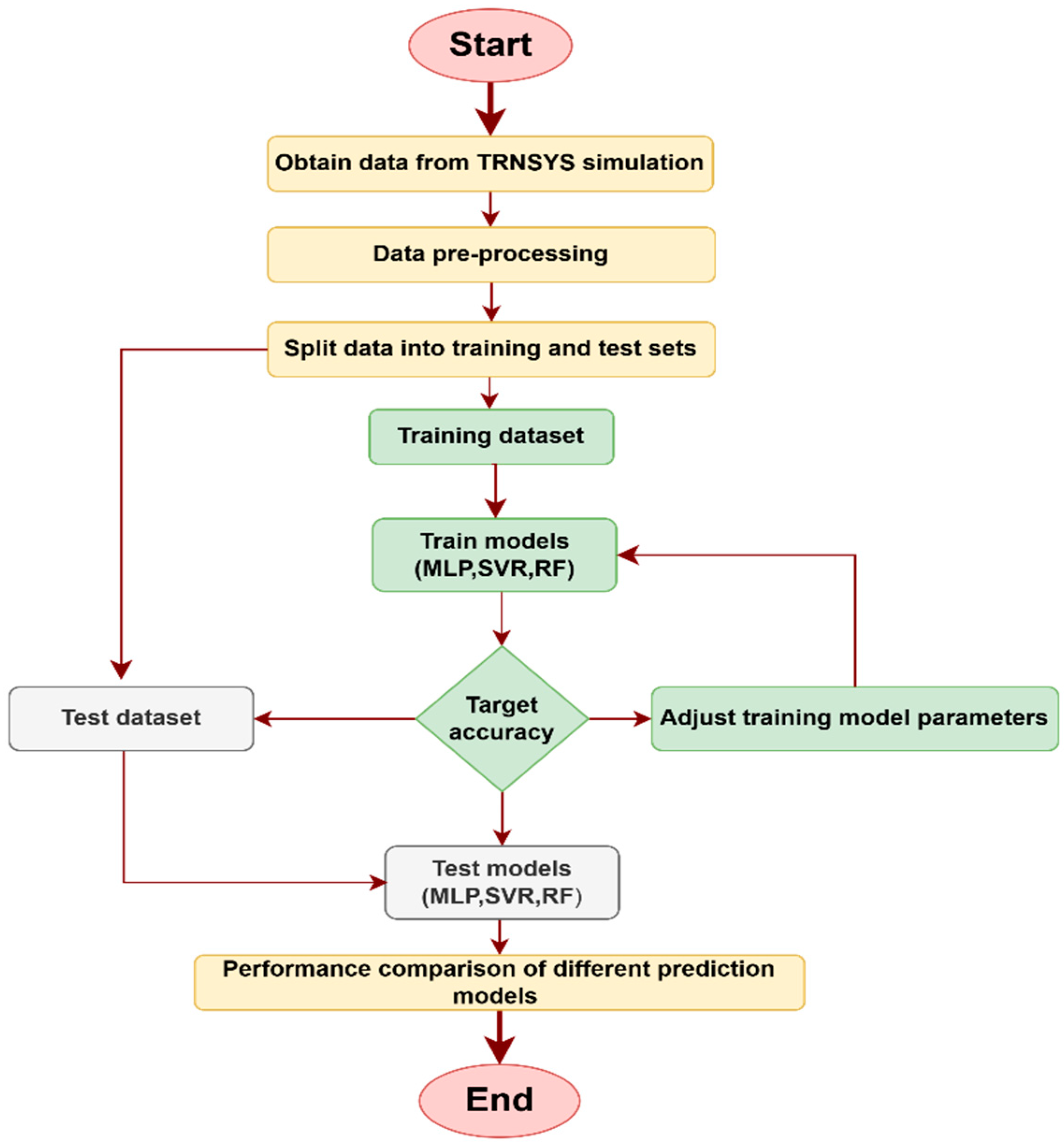
This study focuses on the SAHP system to develop its performance prediction model. The system is installed in a school located in Milan (coordinates: 45°27′39.24″ N, 9°16′48″ E), and the building is a two-story structure, as shown in Figure 1. Due to the difficulty in obtaining long-term operational data for the SAHP systems through field measurements, and the challenges in ensuring the accuracy of such data, the data required for developing the prediction model relies on TRNSYS simulations, with detailed simulation processes referenced in [6].

The heating period extends from 15 October to 14 April of the following year. During this period, the energy produced by the solar collectors and the heat pump is collected in a storage tank connected to the heat dissipation terminal (see Figure 2a). In the non-heating season, due to insufficient energy demand, the hot water produced by the solar collectors flows into the geothermal probes (see Figure 2b). In this way, the intermittent solar energy collected and stored during the summer can be utilized during the peak heating demand in winter. To investigate the impact of the number of probes and the area of solar collectors on the performance of the SAHP system, this study designed 12 different simulation experiments. Specifically, the number of probes was set to 10, 15, 20, and 25, while the areas of the solar collectors were set to 0, 30, and 40 square meters. The time step for the TRNSYS simulation was set to 1 h, with a total simulation duration of 15 years. Considering the excessively large total data volume, this study extracted 8% of the data, amounting to 17,470 data points, to construct the database required to develop the prediction model.

3. Methodology

3.1. Machine Learning Method

Machine learning (ML) is a branch of artificial intelligence (AI). ML algorithms analyze and learn from large datasets, automatically extracting patterns and regularities, which can then be used for tasks such as prediction, classification, clustering, and dimensionality reduction [18]. ML algorithms are categorized into three main types: supervised learning, unsupervised learning, and reinforcement learning [19]. Fundamental machine learning algorithms include linear regression, SVM, KNN, logistic regression, decision trees, k-means clustering, RF, naive Bayes, dimensionality reduction techniques, and gradient boosting [20,21]. With the rapid development of ML, the concept of integrating heat pump systems with ML technology has become increasingly feasible, effective, and necessary, offering vast potential for application [22]. The prediction of COP is fundamentally a regression problem, where effective solutions rely on ML algorithms trained on historical data to uncover the relationships between input variables (features) and output variables (targets). To effectively capture the complex, nonlinear relationships between these features and targets, this study employs MLP, SVM, and RF algorithms to analyze the performance of the SHAP system. The MLP model can be customized to specific datasets and problem requirements by adjusting the number of layers and neurons per layer, thereby enhancing predictive accuracy. The SVM model, with its ability to apply various kernel functions—such as linear, polynomial, and radial basis kernels—offers robust handling of nonlinear data and adapts to diverse data distributions. Additionally, RF, by aggregating predictions from multiple decision trees, achieves superior accuracy compared to single decision trees, while also mitigating overfitting and improving model generalizability.

3.1.1. MLP Algorithm with Back Propagation (MLP Neural Network)

The MLP is a type of feedforward ANN commonly utilized in machine learning and deep learning [23], and the layers and structure of the MLP algorithm used for COP prediction as depicted in Figure 3. An MLP-NN consists of an input layer, one or more hidden layers, and an output layer [24]. Each neuron in one layer is fully connected to every neuron in the next layer. The input layer receives the input data, with each neuron representing one input feature. The number of neurons in each hidden layer is adjustable, allowing for an increase in the complexity of the model by modifying the number of layers and neurons in each. Neurons in these layers apply activation functions to introduce non-linearity. The output layer produces the final output, with each neuron representing one predicted value. MLPs are trained using the backpropagation algorithm, which computes the error and propagates it back through the network to update weights and biases, thereby minimizing the loss function; so, it could enable the MLP to approximate any function by adjusting the values of weights and biases [25].

3.1.2. SVR Algorithm

SVR is an extension of SVM for regression tasks [26], was first introduced by Vapnik [27]. For a given training dataset ${\{(x_i,y_i)\}}_{i=1}^n$, where $x_i$ is the input vector and $y_i$ is the corresponding output value, the goal of SVR is to find a function f(x) with an ϵ-insensitive loss function to approximate the relationship between input and output variables:

$$f\left(x\right)=w\cdot \Phi \left(x\right)+b$$

(1)

where x ∈ Rⁿ, y ∈ R, $\Phi$ is a non-linear transformation that maps input data from the original low-dimensional space Rⁿ to a higher-dimensional space, or infinite-dimensional. The purpose of introducing transformation $\Phi$ is to find a function in the higher-dimensional space to fit the data effectively. w ∈ Rⁿ is the weight vector, and b ∈ R is the bias term. ϵ is a region around the predicted value f(x) set by humans. If the prediction f(x) is within ϵ distance of the actual target value y, the loss is zero. If the prediction error exceeds ϵ, the loss is the magnitude of the error minus ϵ. This means that only the part of the error that exceeds ϵ contributes to the loss. The ϵ insensitive loss function can be defined as:

$$Lϵ(y,f(x))=\left\{\begin{array}{cc}0\hfill & \hfill if\left|y-f\left(x\right)\right| \le ϵ \\ \left|y-f\left(x\right)\right|-ϵ\hfill & \hfill otherwise\end{array}\right..$$

(2)

The goal of SVR optimization is to find the values of parameters $w$ and b such that the regression function f(x) = $w$⋅$\Phi$(x) + b accurately predicts the target values $y_i$ while minimizing the regression risk:

$$\underset{W,B}{\mathit{min}}{\displaystyle \frac{1}{2}}{\left|\right|w\left|\right|}^2+C{\sum }_{i=1}^{m}Lϵ(f\left(x_i\right),y_i).$$

(3)

To prevent overfitting and ensure better convergence during model training, slack variables are introduced. Slack variables relax the strict requirement that every training sample must lie within the margin defined by the support vectors. After introducing slack variables, Equation (3) can be rewritten as:

Target function:

$$\underset{W,B}{min}{\displaystyle \frac{1}{2}}{\left|\right|w\left|\right|}^2+C{\sum }_{i=1}^m({\xi }_i+{\xi }_i^{\mathrm{*}}).$$

Subject to:

$$\left\{\begin{array}{c}{y}_i-f(x_i)\le ϵ+{\xi }_i\\ f(x_i)-y_i\le ϵ+{\xi }_i^{*}\\ {\xi }_i,{\xi }_i^{*}\ge 0\end{array}\right..$$

(4)

For dual optimization problems, the weights can be expressed as follows Equation (5)

$$w={\sum }_{i=1}^l({\alpha }_i-{\alpha }_i^{*})\hspace{1em}\Phi (x_i).$$

(5)

By substituting Equation (5) into Equation (1), the target function can be rewritten as:

$$f(x)={\sum }_{i=1}^l({\alpha }_i-{\alpha }_i^{*})\Phi (x_i)\Phi (x)+b.$$

(6)

Kernel functions k ($x_i$, x) = $\Phi$($x_i$)$\Phi$(x) enable machine learning algorithms to operate effectively in high-dimensional feature spaces by implicitly mapping the original input space Rn to a potentially infinite-dimensional feature space, without explicitly computing the mapping $\Phi$(x). After introducing the kernel function, Equation (6) can be rewritten as

$$f(x)={\sum }_{i=1}^l({\alpha }_{\mathrm{i}}-{\alpha }_i^{\mathrm{*}})\mathrm{k} (x_i,x)+b.$$

(7)

3.1.3. Random Forest

RF is an ensemble learning method proposed by Leo Breiman and Adele Cutler in 2001, widely used for classification, regression, and other tasks [28]. This method improves the predictive performance and stability of models by constructing and combining multiple decision trees [29]. A decision tree is a tree-structured predictive model composed of a root node, internal nodes, and leaf nodes. The root node is the starting point of the tree, containing the entire dataset and performing the initial split based on a selected feature. Internal nodes lie below the root node, with each node representing a decision and split on a particular feature. Leaf nodes are the terminal nodes of the tree, representing the final classification result or regression value. In regression tasks, a decision tree splits the data at each node by selecting the optimal feature and split point to minimize the MSE between the resulting subsets. When the number of samples at a node falls below a predefined minimum, or when further splitting does not significantly reduce the MSE, the splitting process stops, and the node is marked as a leaf node. The output value of the leaf node is the mean of the target variable within that subset. RF enhances prediction accuracy by combining the results of multiple decision trees without significantly increasing computation time [30]. By employing bootstrap sampling to generate multiple different subsets of the original training data randomly, each decision tree is trained on a unique sample set. This randomness effectively prevents the overfitting issue common to individual decision trees. Additionally, RF demonstrates strong robustness to missing values and noisy data. These characteristics make RF a powerful and widely applied machine learning algorithm that is suitable for various real-world applications.

3.2. Model Performance Evaluation

In this study, MAE and RMSE are utilized as evaluation metrics to assess the model’s performance. MAE is the average of the absolute differences between predicted and actual values, indicating the average magnitude of errors in predictions. RMSE is defined as the square root of the average of the squared differences between predicted values and actual values, providing a measure of the difference between the predicted values and the actual values. Lower values of RMSE and MAE indicate more accurate model prediction performance.

$$\mathit{MAE}={\displaystyle \frac{1}{n}}{\sum }_{i=1}^n|y_{i }-\widehat{y_i}|$$

(8)

$$\mathit{RMSE}\sqrt{{{\displaystyle \frac{1}{n}}{\sum }_{i=1}^n(y_{i }-\widehat{y_i})}^2}$$

(9)

where $y_i$ represents the actual values, $\widehat{y_i}$ represents the predicted values, and n is the number of observations.

4. Machine Learning Modeling

The ML modeling process is illustrated in Figure 4. The dataset for prediction was generated using TRNSYS, followed by data preprocessing, including outlier detection and removal as well as normalization. The pre-processed dataset was then split into a training set (70%) and a test set (30%). The training set was used to train three models: MLP, SVM, and RF. Hyperparameter optimization was performed to identify the best hyperparameter combinations for each model. Finally, the trained optimal models were validated on the test set, and the predictive performance of the three models was compared.

4.1. Database and Data Preprocessing

The database for this study is derived from a long-term dynamic TRNSYS simulation spanning 15 years on a SAHP system. The dynamic analysis performed by Ballerini et al. [6] aims to investigate the potential use of solar thermal collectors to supply energy to the borehole field employed by the heat pump during the summer period, when there is no need for space heating. Different scenarios were considered, varying the number of probes and the area of solar thermal collectors.

4.1.1. Data Outliers and Detection

The original dataset frequently includes outlier values, which can significantly undermine the dataset’s quality and diminish the accuracy and robustness of subsequent models. Therefore, the detection and removal of outliers is imperative for enhancing database quality. The interquartile range (IQR) method, a robust statistical method, is particularly effective in identifying and eliminating outliers from original data.

4.1.2. Min–Max Normalization Cop (Output)

Normalization is also a critical step in data preprocessing, ensuring that each data point is scaled to fall between 0 and 1, which effectively reduces differences between features. This process accelerates model training, improves model stability, and enhances generalization capabilities. X is the original feature value,${ X}_{min }$ is the minimum value of the feature, and $X_{max}$ is the maximum value of the feature and X′ is the normalized value.

$${\mathrm{X}}^{\prime }={\displaystyle \frac{X-X_{min}}{X_{max-{ X}_{min}}}}$$

(10)

4.2. Modeling Optimization

For models built, the number of probes, the areas of solar panels, the electricity consumed, and the energy provided by solar collectors are selected as predictor variables (inputs), and the predicted value (output) of the model is the COP of the SAHP system. Our optimization goal is to minimize the values of MAE and RMAE. SVR, MLP with BP, and RF algorithms are chosen to build models.

Extensive experiments have been conducted to enhance the accuracy of the MLP prediction model. All model parameters are detailed in

Table 1. Parameter configuration of MLP model.

Optimized Parameters	Values
The number of layers	1, 2, 3, 4, 5
The number of nodes at each layer	4, 5, 6, 7, 8, 9, 10, 11, 12
Activation function	Sigmoid
Momentum	0.1, 0.2, 0.3, 0.4, 0.5, 0.6, 0.7, 0.8, 0.9, 0.99
Learning rate	0.001, 0.01, 0.1, 0.2, 0.3, 0.5
Number of epochs	500, 800
Batch size	100, 1000

. It is crucial to select the optimal number of hidden layers and the number of neurons in each layer. Through manual adjustments of the network architecture, it was determined that a model with four hidden layers, each containing nine neurons, achieves optimal performance. The experimental results are summarized in

Table 2. Accuracy of MLP prediction model with different of the number of layers.

Output	Number of Layers		Accuracy [%]
		MAE	RMSE	MSE	RMSE
		(Train)	(Train)	(Test)	(Test)
Coefficient of performance	1	6.54	9.12	6.33	8.67
	2	6.11	9.13	5.84	8.64
	3	5.82	8.84	5.56	8.34
	4	5.57	8.85	5.47	8.33
	5	22.83	27.36	22.8	27.26

and

Table 3. Accuracy of MLP prediction model with different of the number of nodes.

Output	Number of Nodes		Accuracy [%]
		MAE	RMSE	MSE	RMSE
		(Train)	(Train)	(Test)	(Test)
Coefficient of performance	4	5.57	8.85	5.47	8.33
	5	5.84	8.87	5.61	8.29
	6	5.77	9.02	5.51	8.51
	7	5.73	8.83	5.47	8.31
	8	5.52	8.68	5.27	8.18
	9	5.5	8.74	5.24	8.21
	10	5.58	8.78	5.33	8.25
	11	5.68	8.82	5.42	8.3
	12	5.53	8.75	5.28	8.22

. The selection and tuning of hyperparameters are also critical to the model’s performance. Properly setting and optimizing hyperparameters can significantly enhance the model’s accuracy and training efficiency. Following the determination of the number of layers and neurons per layer, the hyperparameters that require further optimization include momentum, learning rate, batch size, and the number of iterations. Introducing momentum can accelerate convergence and reduce oscillations, with the optimal momentum value typically found between 0 and 1. To determine the best momentum value, the momentum was incrementally increased from 0.1 to 0.99. The learning rate dictates the step size for each weight update. A learning rate that is too high may prevent the model from converging and cause significant fluctuations in the loss function, while a learning rate that is too low can result in slow convergence and potentially lead to being trapped in a local optimum. The learning rate gradually increased from 0.001 to 0.5. Batch size refers to the number of training samples used in each iteration. A larger batch size can provide higher computational efficiency and more accurate gradient estimates but requires more memory and may lead to model overfitting. Conversely, a smaller batch size offers lower computational efficiency and noisier gradient estimates but can help the model escape local optima. The number of iterations indicates how many times the entire training set is used for training. Insufficient iterations may cause underfitting, while excessive iterations can lead to overfitting. After conducting 35 experiments, the optimal hyperparameter configuration was determined as follows: momentum is set to 0.2, the learning rate is set to 0.3, the batch size is set to 100, and the number of epochs is set to 500.

To optimize the performance of the SVR model, it is crucial to select an appropriate kernel function, C (regularization parameter), and ε (error tolerance parameter); the detailed parameter configuration of the SVR model is shown in

Table 4. Parameter configuration of SVR model.

Optimized Parameters	Values
Kernel function	PUK, RBF, Poly
C	1, 2, 5, 8, 10
ε (Epsilon)	10−1, 10−2, 10−3, 10−4
σ (Sigma)	0.1, 0.5, 1,2
ω (Omega)	1, 1.5, 2, 3

. Firstly, a suitable kernel function should be chosen to map input data to a high-dimensional feature space. This study evaluated several kernel functions, including the polynomial kernel, RBF kernel, and PUK kernel, and the predictive accuracy of the SVR model under each kernel function is summarized in

Table 5. Accuracy of SVR prediction model using different kernel functions.

Output	Kernel Function		Accuracy [%]
		MAE	RMSE	MSE	RMSE
		(Train)	(Train)	(Test)	(Test)
Coefficient of performance	PUK	5.91	7.71	5.89	7.75
	RBF	6.97	9.8	6.79	9.39
	Poly	21.49	25.53	21.58	25.59

. The results show that the PUK kernel function demonstrates superior performance. The parameters σ and θ of the kernel function significantly affect the model’s complexity, fitting capacity, and generalization performance. The parameter σ controls the width of the kernel function. Larger σ values increase the range of influence of the kernel function, while smaller σ values decrease it. The parameter ω adjusts the shape of the kernel function, allowing the kernel to fit the data distribution better. In this study, σ was tested at values of 0.1, 0.5, 1, and 2, with the model performing best when σ is set to 0.1. Likewise, ω was tested at values of 1, 1.5, 2, and 3, and the model showed the best performance when ω is set to 1. After selecting an appropriate kernel function and completing the optimization of its parameters, other parameters that need to be optimized include C and ε. The C parameter balances the trade-off between achieving a low training error and a low model complexity. A higher C value emphasizes minimizing the training error, potentially leading to overfitting, while a lower C value results in a smoother decision surface and may cause underfitting. Various values, including 1, 2, 5, 8, and 10, were tested for C, with the results indicating that the model achieved the lowest MSE when C was established at 10. ε defines a margin of tolerance where no penalty is given for errors. It determines the width of the ε-insensitive zone used to fit the training data. Larger values of ε result in fewer support vectors and a smoother function, while smaller values make the function fit the data more closely. To determine an optimal ε, this study explored a range of values from 10⁻¹ to 10⁻⁴, ultimately identifying that the model exhibited superior performance when ε was configured at 10⁻⁴. Following an extensive series of 19 experiments, the optimal hyperparameter configuration for the SVR model was determined as follows: C is set to 10, ε is 10⁻⁴, ω), and σ is 0.1.

The accuracy of the RF model is significantly influenced by the maximum depth of the decision trees, the maximum number of features, and the number of decision trees, and the parameter settings for the RF model are comprehensively described in

Table 6. Parameter configuration of RF model.

Optimized Parameters	Values
Max depth	10, 20, 30, 35, 40, 60
Max-feature	1, 2, 3
The number of trees	100, 300, 500

. When the maximum depth of the trees is low, the model structure is simple and less complex. In this scenario, the model may not sufficiently capture the complex patterns in the data, leading to underfitting. As the maximum depth of the trees increases, the model structure becomes more complex, allowing it to capture finer details and complex patterns in the data. However, deeper trees are also more prone to overfitting the training data, capturing noise and outliers, reducing the model’s generalization ability, and decreasing the test set’s accuracy. In this study, the maximum depth of the decision trees was manually adjusted, increasing incrementally from 10 to 60. Experimental results indicate that when the depth reached 35, the model’s MSE was minimized. Regarding max features, when this parameter is set to a lower value, each tree uses only a subset of features for splitting. This randomness helps reduce the model’s dependency on specific features, thereby lowering the risk of overfitting. Although smaller max features can decrease overfitting, it may also lead to the omission of some key features, preventing the model from thoroughly learning the complex patterns in the data and potentially decreasing overall accuracy. When max features are set to a higher value, the model can utilize more information for splitting, usually improving the accuracy of individual trees. However, this also increases the risk of overfitting, especially when the number of features is large, and the number of samples is small. The maximum number of features was gradually increased from 1 to 3, and results show that when the maximum number of features was set to 3, the MSE on the test set reached its lowest value. Moreover, the number of decision trees is crucial in determining the model’s accuracy. The greater the number of trees, the more stable and accurate the model tends to be, as more trees can reduce the model’s variance and minimize the impact of individual tree prediction errors on the overall model. However, increasing the number of trees also raises computational costs and time. By manually increasing the number of decision trees, it was found that the model performed optimally when the number of trees reached 500. Through a series of 12 experimental runs, the optimal configuration for the RF model was established as comprising 500 decision trees, a maximum depth of 35, and a maximum of three features. This configuration effectively balances model complexity with computational resources, significantly enhancing both the accuracy and generalization capability of the model.

5. Result and Discussion

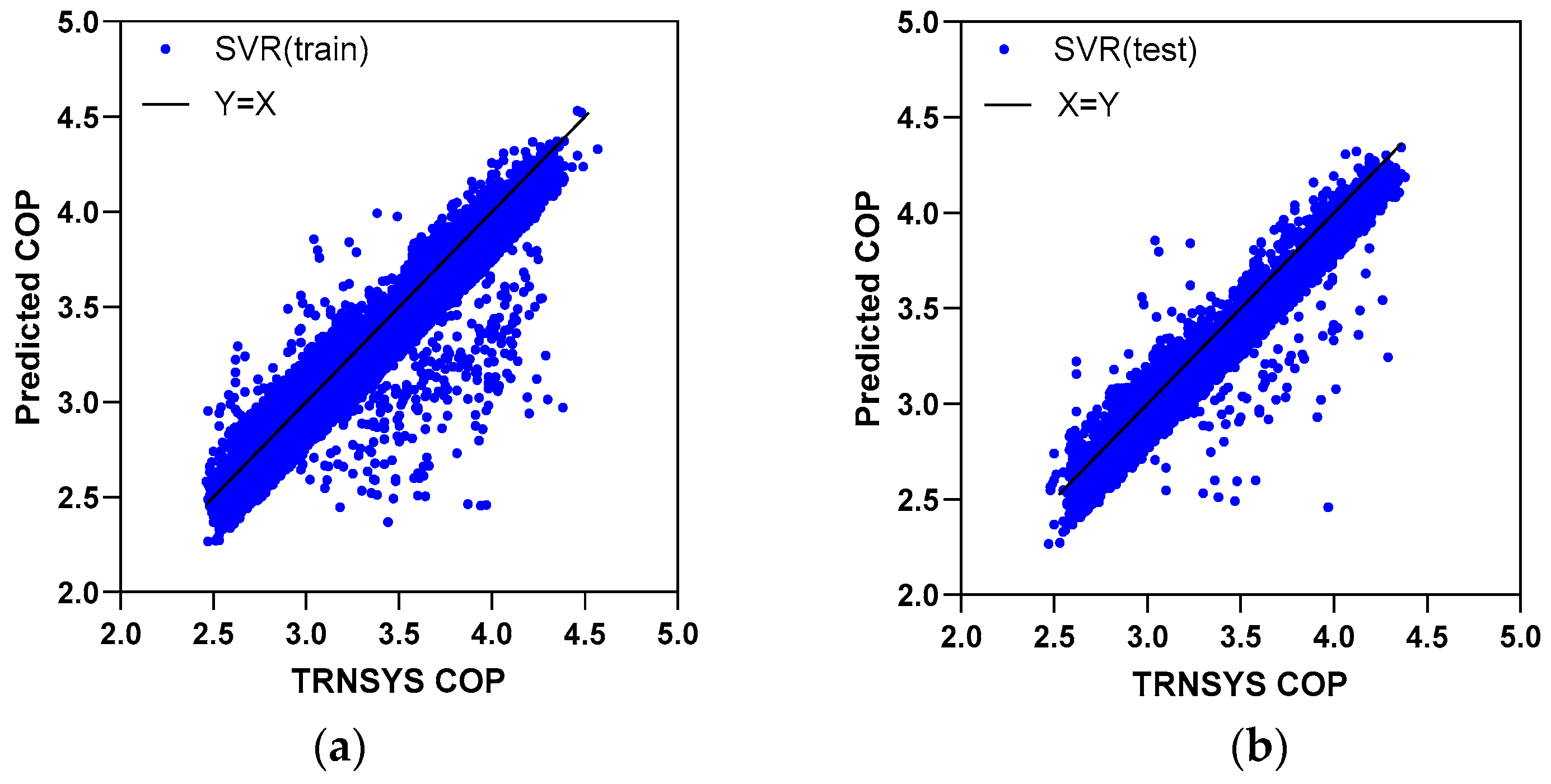
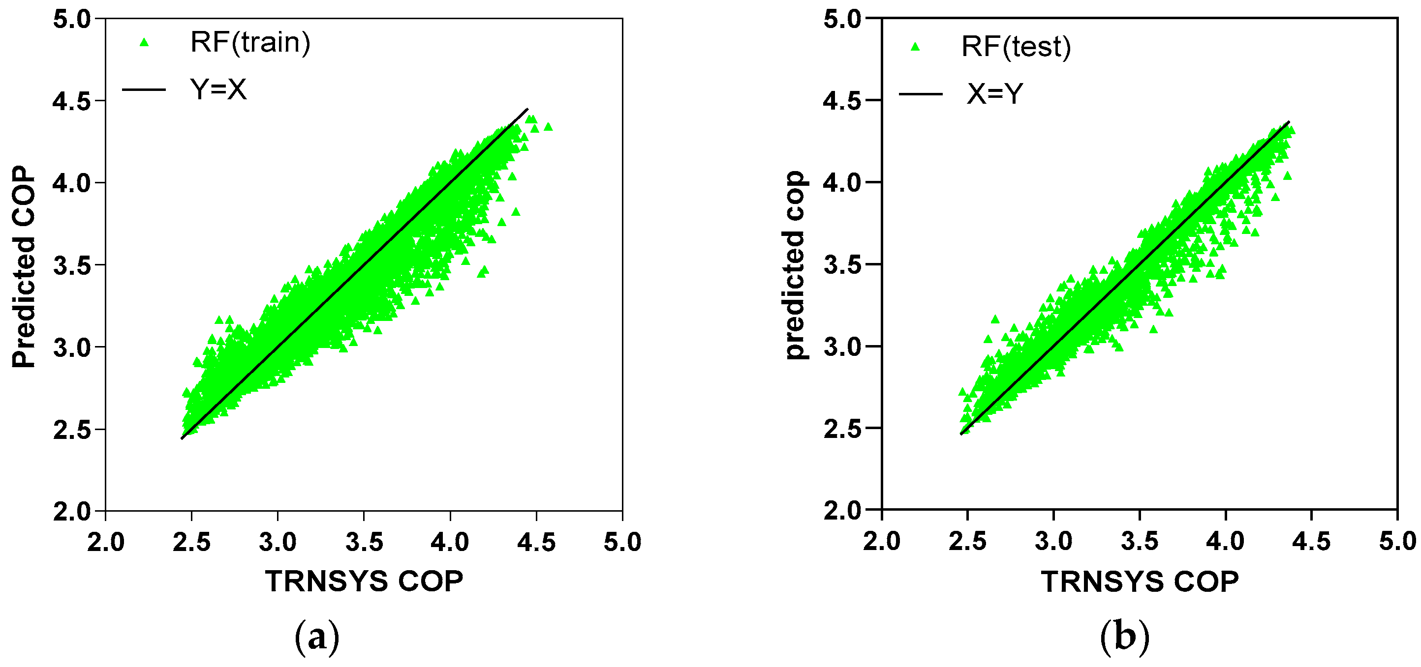
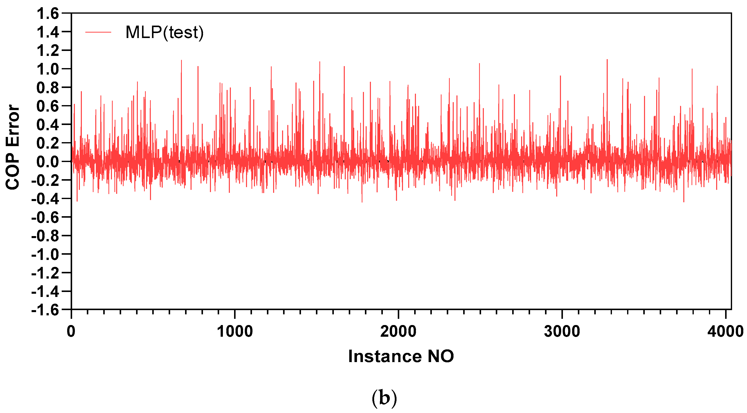
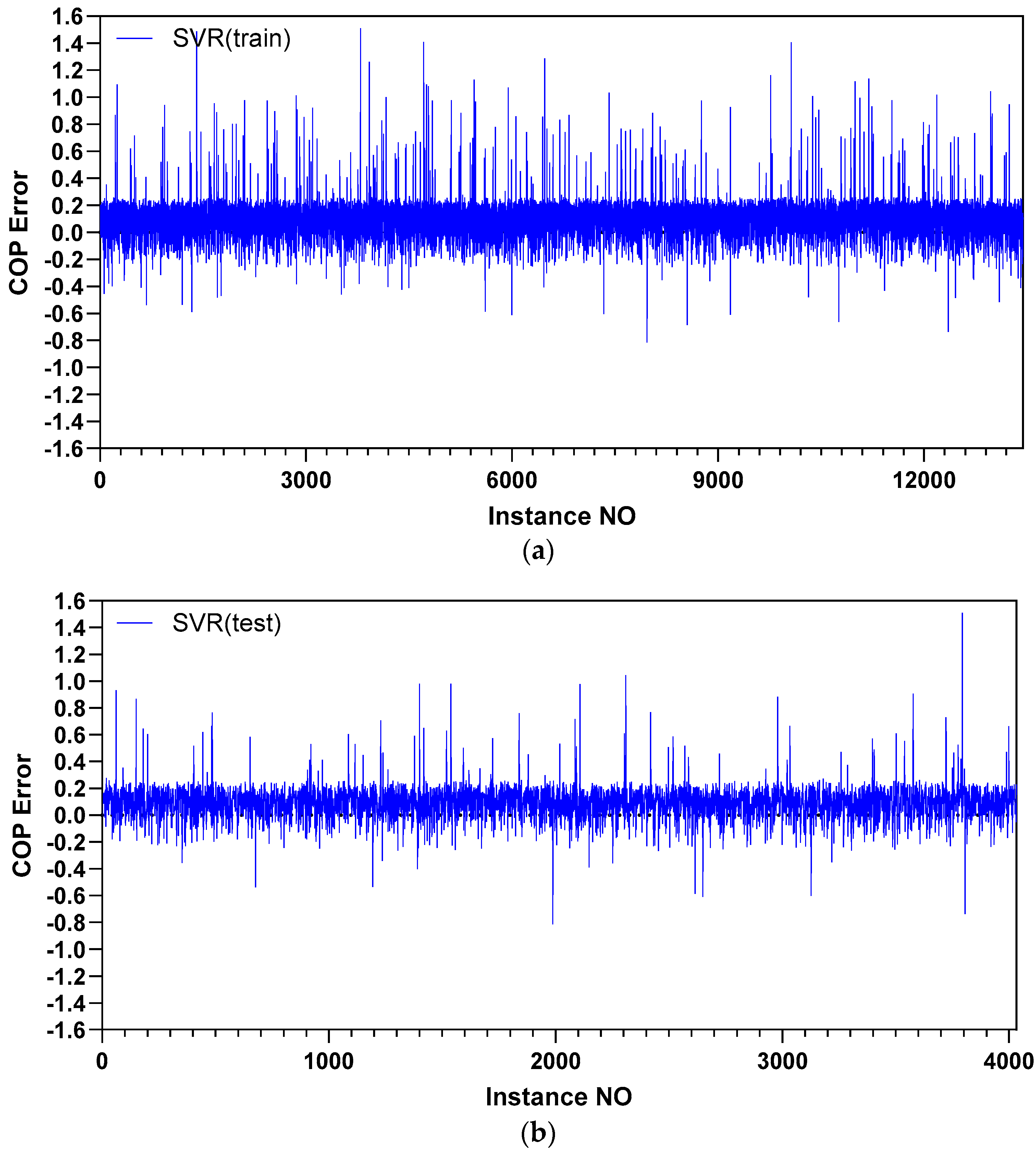
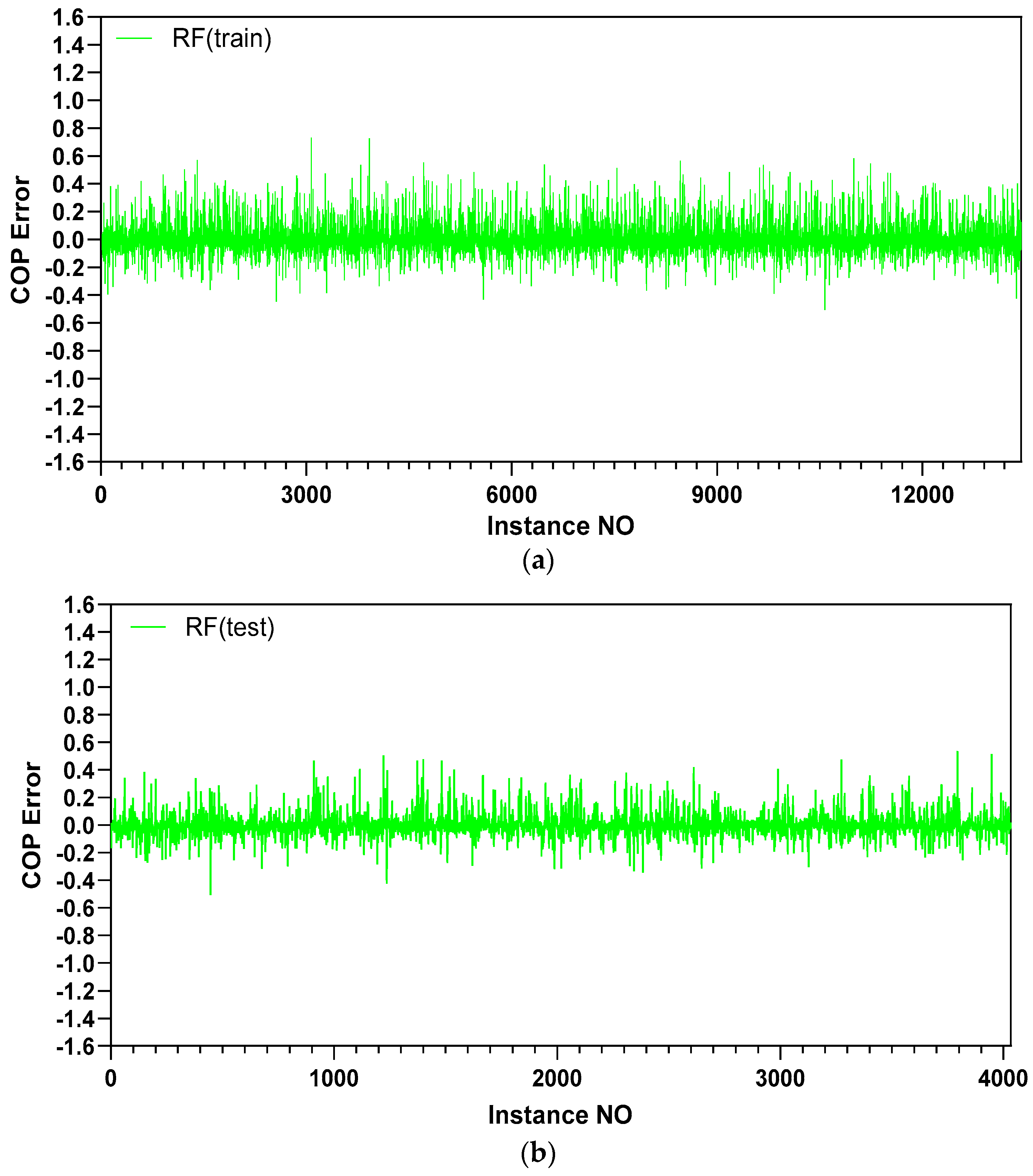
5.1. Prediction Accuracy

In this study, MLP, SVM, and RF models have been used to predict the COP of SAHP systems. To evaluate the accuracy of the models, MAE and RMSE are used as key performance indicators. Typically, models with lower MAE and RMSE values are considered to have higher predictive accuracy. In the performance evaluation of the training set, the MLP model exhibited a MAE of 5.5% and a RMSE of 8.74%. The SVR model achieved an MAE of 5.91% and an RMSE of 7.71%, while the RF model attained an MAE of 2.42% and an RMSE of 4.01%. The evaluation results on the test set indicate that the MLP model had an MAE of 5.24% and an RMSE of 8.21%. Similarly, the SVR model showed an MAE of 5.89% and an RMSE of 7.75%. Meanwhile, the RF model demonstrated an MAE of 2.35% and an RMSE of 3.84%, and

Table 7. Accuracy of prediction models.

Output	Prediction Model		Accuracy [%]
		MAE	RMSE	MSE	RMSE
		(Train)	(Train)	(Test)	(Test)
Coefficient of performance	MLP	5.5	8.74	5.24	8.21
	SVR	5.91	7.71	5.89	7.75
	RF	2.42	4.01	2.35	3.84

summarizes the MAE and RMSE values for the three models on both the training and testing datasets. The results indicate that the RF models exhibit superior predictive accuracy compared to the MLP and SVR models. Figure 5, Figure 6 and Figure 7 illustrate the comparison between the predicted COP values of the models and the TRNSYS simulated COP values. The prediction results of all three models are highly consistent with the TRNSYS simulation results. Additionally, a Y = X line is added in the figures, with data points closer to this line indicating higher prediction accuracy. It is evident from the figures that the RF model’s data points are the closest to the Y = X line among the three models. Figure 8, Figure 9 and Figure 10 illustrate the differences between the predicted values and the TRNSYS-simulated values for the three models in both the training and testing datasets. In these figures, the error expression presented on the y-axis shows the difference between the TRNSYS simulation and the predicted COP values for the entire dataset. Prediction errors originating from MLP, SVM, and RF machine learning methods are displayed with red, blue, and green lines, respectively. Closeness to the zero point indicates good prediction performance, while large fluctuations from the zero point indicate poor prediction performance. In the training set, the maximum errors between the predicted values and TRNSYS-simulated values for the MLP, SVR, and RF models are 1.34, 1.51, and 0.73, respectively. In the testing set, the maximum error for the MLP model is 1.10, for the SVM model is 1.51, and for the RF model is 0.54. In contrast, the RF model exhibits significantly smaller fluctuations in both the training and testing sets compared to the MLP and SVR models. Overall, the RF model demonstrates the best performance among the three predictive models, indicating it is the most reliable and accurate model.

5.2. Training Time

Computational efficiency is another important factor to consider when evaluating a model. The time required to build the three models is presented in

Table 8. Modeling time of prediction models.

Prediction Model	Values [s]
MLP	33.01
SVR	67.67
RF	6.57

. The MLP model takes 33.01 s to build, while the SVM model requires 67.67 s. In contrast, the RF model is built in only 6.57 s. Compared to the MLP and SVM models, the RF model demonstrates a significantly shorter training time. This is likely because, although the RF comprises multiple decision trees, these trees can be generated in parallel. Since the construction of each decision tree is independent of the others, the RF model benefits from parallel computation on multi-core processors, thus accelerating the training process. Additionally, the RF model has a relatively simpler structure compared to the MLP model, requiring fewer computational resources, which further contributes to its shorter training time.

6. Conclusions

This study developed COP prediction models for SAHP systems using data-driven intelligent algorithms. Three algorithms, namely MLP, SVR, and RF, were evaluated regarding prediction accuracy and computational efficiency. The evaluation metrics included MAE and RMSE for accuracy, while modeling time was used to assess computational efficiency. A methodological approach was followed and described in detail. The analysis results indicate that data-driven algorithms are highly effective in predicting the performance of SAHP systems.

It can be concluded that the RF model outperformed the MLP and SVR models in both accuracy and computational efficiency. Specifically, the RF model achieved an MAE of 2.42% and an RMSE of 4.01% on the training set, and an MAE of 2.35% and an RMSE of 3.84% on the test set, with a modeling time of only 6.57 s. These findings suggest that the RF model is an effective method for predicting the performance of the SAHP system and also provide a solid foundation for the future development of real-time performance management systems for SAHP.

Future work will focus on optimizing the system design based on the RF prediction model. This includes exploring the optimal configuration of the solar panel area and the number of probes to further reduce costs and enhance the system’s energy efficiency.

References

1. IEA. World Energy Outlook. 2019. Available online: https://www.iea.org/weo2019/ (accessed on 2 December 2019).
2. Angelidis, O.; Ioannou, A.; Friedrich, D.; Thomson, A.; Falcone, G. District heating and cooling networks with decentralised energy substations: Opportunities and barriers for holistic energy system decarbonisation. Energy 2023, 269, 126740. [Google Scholar] [CrossRef]
3. Badiei, A.; Akhlaghi, Y.G.; Zhao, X.; Shittu, S.; Xiao, X.; Li, J.; Fan, Y.; Li, G. A chronological review of advances in solar assisted heat pump technology in 21st century. Renew. Sustain. Energy Rev. 2020, 132, 110132. [Google Scholar] [CrossRef]
4. Razavi, S.H.; Ahmadi, R.; Zahedi, A. Modeling, simulation and dynamic control of solar assisted ground source heat pump to provide heating load and DHW. Appl. Therm. Eng. 2018, 129, 127–144. [Google Scholar] [CrossRef]
5. Maranghi, F.; Gosselin, L.; Raymond, J.; Bourbonnais, M. Modeling of solar-assisted ground-coupled heat pumps with or without batteries in remote high north communities. Renew. Energy 2023, 207, 484–498. [Google Scholar] [CrossRef]
6. Ballerini, V.; Rossi di Schio, E.; Valdiserri, P.; Naldi, C.; Dongellini, M. A Long-Term Dynamic Analysis of Heat Pumps Coupled to Ground Heated by Solar Collectors. Appl. Sci. 2023, 13, 7651. [Google Scholar] [CrossRef]
7. Ballerini, V.; Lubowicka, B.; Valdiserri, P.; Krawczyk, D.A.; Sadowska, B.; Kłopotowski, M.; di Schio, E.R. The Energy Retrofit Impact in Public Buildings: A Numerical Cross-Check Supported by Real Consumption Data. Energies 2023, 16, 7748. [Google Scholar] [CrossRef]
8. Franco, A.; Miserocchi, L.; Testi, D. HVAC energy saving strategies for public buildings based on heat pumps and demand controlled ventilation. Energies 2021, 14, 5541. [Google Scholar] [CrossRef]
9. Adelekan, D.S.; Ohunakin, O.S.; Paul, B.S. Artificial intelligence models for refrigeration, air conditioning and heat pump systems. Energy Rep. 2022, 8, 8451–8466. [Google Scholar] [CrossRef]
10. Wang, Y.; Li, W.; Zhang, Z.; Shi, J.; Chen, J. Performance evaluation and prediction for electric vehicle heat pump using machine learning method. Appl. Therm. Eng. 2019, 159, 113901. [Google Scholar] [CrossRef]
11. Afram, A.; Janabi-Sharifi, F.; Fung, A.S.; Raahemifar, K. Artificial neural network (ANN) based model predictive control (MPC) and optimization of HVAC systems: A state of the art review and case study of a residential HVAC system. Energy Build. 2017, 141, 96–113. [Google Scholar] [CrossRef]
12. Ahmed, N.; Assadi, M.; Ahmed, A.A.; Banihabib, R. Optimal design, operational controls, and data-driven machine learning in sustainable borehole heat exchanger coupled heat pumps: Key implementation challenges and advancement opportunities. Energy Sustain. Dev. 2023, 74, 231–257. [Google Scholar] [CrossRef]
13. Esen, H.; Inalli, M.; Sengur, A.; Esen, M. Modeling a ground-coupled heat pump system by a support vector machine. Renew. Energy 2008, 33, 1814–1823. [Google Scholar] [CrossRef]
14. Xu, X.; Liu, J.; Wang, Y.; Xu, J.; Bao, J. Performance evaluation of ground source heat pump using linear and nonlinear regressions and artificial neural networks. Appl. Therm. Eng. 2020, 180, 115914. [Google Scholar] [CrossRef]
15. Eom, Y.H.; Chung, Y.; Park, M.; Hong, S.B.; Kim, M.S. Deep learning-based prediction method on performance change of air source heat pump system under frosting conditions. Energy 2021, 228, 120542. [Google Scholar] [CrossRef]
16. Shin, J.H.; Cho, Y.H. Machine-learning-based coefficient of performance prediction model for heat pump systems. Appl. Sci. 2021, 12, 362. [Google Scholar] [CrossRef]
17. Chesser, M.; Lyons, P.; O’Reilly, P.; Carroll, P. Air source heat pump in-situ performance. Energy Build. 2021, 251, 111365. [Google Scholar] [CrossRef]
18. Alpaydin, E. Introduction to Machine Learning; MIT Press: Cambridge, MA, USA, 2020. [Google Scholar]
19. Ahmad, T.; Zhu, H.; Zhang, D.; Tariq, R.; Bassam, A.; Ullah, F.; AlGhamdi, A.S.; Alshamrani, S.S. Energetics Systems and artificial intelligence: Applications of industry 4.0. Energy Rep. 2022, 8, 334–361. [Google Scholar] [CrossRef]
20. Yan, L.; Hu, P.; Li, C.; Yao, Y.; Xing, L.; Lei, F.; Zhu, N. The performance prediction of ground source heat pump system based on monitoring data and data mining technology. Energy Build. 2016, 127, 1085–1095. [Google Scholar] [CrossRef]
21. Bishop, C.M.; Nasrabadi, N.M. Pattern Recognition and Machine Learning; Springer: New York, NY, USA, 2006. [Google Scholar]
22. Zhou, S.L.; Shah, A.A.; Leung, P.K.; Zhu, X.; Liao, Q. A comprehensive review of the applications of machine learning for HVAC. DeCarbon 2023, 2, 100023. [Google Scholar] [CrossRef]
23. Abiodun, O.I.; Jantan, A.; Omolara, A.E.; Dada, K.V.; Mohamed, N.A.; Arshad, H. State-of-the-art in artificial neural network applications: A survey. Heliyon 2018, 4, e00938. [Google Scholar] [CrossRef]
24. Haykin, S. Neural Networks: A Comprehensive Foundation; Prentice Hall PTR: Hoboken, NJ, USA, 1998. [Google Scholar]
25. Guo, Y.; Wang, J.; Chen, H.; Li, G.; Liu, J.; Xu, C.; Huang, R.; Huang, Y. Machine learning-based thermal response time ahead energy demand prediction for building heating systems. Appl. Energy 2018, 221, 16–27. [Google Scholar] [CrossRef]
26. Zhang, X.; Wang, E.; Liu, L.; Qi, C. Machine learning-based performance prediction for ground source heat pump systems. Geothermics 2022, 105, 102509. [Google Scholar] [CrossRef]
27. Vapnik, V. Statistical Learning Theory; John Wiley & Sons: Hoboken, NJ, USA, 1998; Volume 2, pp. 831–842. [Google Scholar]
28. Breiman, L. Random forests. Mach. Learn. 2001, 45, 5–32. [Google Scholar] [CrossRef]
29. Liaw, A.; Wiener, M. Classification and regression by randomForest. R News 2002, 2, 18–22. [Google Scholar]
30. Lu, S.; Li, Q.; Bai, L.; Wang, R. Performance predictions of ground source heat pump system based on random forest and back propagation neural network models. Energy Convers. Manag. 2019, 197, 111864. [Google Scholar] [CrossRef]
Figure 1. Three-dimensional view of the building under investigation (a) and school plan (b) [6].
Energies 17 05607 g001aEnergies 17 05607 g001b
Figure 2. Plant working conditions in winter (a) and in summer (b); the grey lines represent non-active connections during the specific season [6].
Energies 17 05607 g002
Figure 3. MLP structure for COP prediction.
Energies 17 05607 g003
Figure 4. Flow chart of the machine learning modeling procedure.
Energies 17 05607 g004
Figure 5. Comparison between TRNSYS COP and MLP model predicted COP on the training set (a) and test set (b).
Energies 17 05607 g005
Figure 6. Comparison between TRNSYS COP and SVR model predicted COP on the training set (a) and test set (b).
Energies 17 05607 g006
Figure 7. Comparison between TRNSYS COP and RF model predicted COP on the training set (a) and test set (b).
Energies 17 05607 g007
Figure 8. Differences between TRNSYS COP and MLP model predicted COP on the training set (a) and test set (b).
Energies 17 05607 g008aEnergies 17 05607 g008b
Figure 9. Differences between TRNSYS COP and SVR model predicted COP on the training set (a) and test set (b).
Energies 17 05607 g009
Figure 10. Differences between TRNSYS COP and RF model predicted COP on the training set (a) and test set (b).
Energies 17 05607 g010