Abstract
Cold energy generation is an important part of liquefied natural gas (LNG) cold energy cascade utilization, and existing studies lack a specific descriptive model for LNG cold energy transmission to the AC subgrid. Therefore, this paper proposes a descriptive model for the grid-connected process of cold energy generation at LNG stations. First, the expansion kinetic energy transfer of the intermediate work mass is derived and analyzed in the LNG unipolar Rankine cycle structure, the mathematical relationship between the turbine output mechanical power and the variation in the work mass flow rate and pressure is established, and the variations in the LNG heat exchanger temperature difference, seawater flow rate, and the turbine temperature difference in the cycle system are investigated. Secondly, based on the fifth-order equation of state of the synchronous generator, the expressions of its electromagnetic power, output AC frequency, and voltage were analyzed. Finally, the average equivalent models of the machine-side and grid-side converters are established using a direct-fed grid-connected structure, thus forming a descriptive model of the overall drive process. The ORC model is built in Aspen HYSIS to obtain the time series expression of the torque output of the turbine; based on the ORC output torque, the permanent magnet synchronous generator (PMGSG) as well as the direct-fed grid-connected structure are built in MATLAB/Simulink, and the active power and current outputs of the grid-following-type voltage vector control method and the grid-forming-type power-angle synchronous control method are also verified.
1. Introduction
Transportation of natural gas involves liquefaction, marine transportation, regasification, and finally delivery to the gas load through a pipeline [1,2,3]. In the regasification stage, the cold energy is released by the conversion of liquefied natural gas (LNG) at a temperature of −163 °C to natural gas at 10 °C is 830 kJ/kg [4,5,6]. The low cold temperature and high quality of LNG allow it to be used as a cryogenic source in many fields.
Cold power generation is a part of LNG cold energy utilization, and its working temperature should be kept below −110 °C; in engineering practice, cold power generation and air separation are taken as the first part of cold energy gradient utilization. Existing research on cold energy utilization technology mainly focuses on cold power generation, liquefied air energy storage, and air composition separation. Refs. [7,8] proposed using the cold energy released from LNG regasification to liquefy air and realize liquefied air energy storage. Ref. [9] analyzed the availability of LNG cold energy for regasification in renewable and non-renewable processes; expressions for thermodynamic processes and energy efficiency were also proposed to facilitate the evaluation of the processes. Ref. [10] investigates the structure of LNG cold energy generation in series and parallel combined cycles, which can provide theoretical guidance to improve the problem of too large irreversible heat losses between the heat exchanger mass and the LNG.
The methods used to realize LNG cold power generation mainly include the direct expansion method, Organic Rankine cycle (ORC), Brayton cycle, and Kalina cycle. Existing studies mainly address the problem of low Exergy efficiency by optimizing the scheme or optimizing the parameters. Ref. [11] proposed a combined cycle optimization design with ORC and BC as the top cycle and ORC, BC, and supercritical carbon dioxide power cycle as the low cycle to solve the problem of low net power generation from single-cycle LNG cold energy. Ref. [12] compares the structures of unipolar ORC, parallel ORC, and cascaded ORC. A particle swarm optimization algorithm was used to optimize seven key parameters for 64 fluid combinations at four heat source temperatures to investigate the relationship between the optimal work masses and parameters as a function of structure and heat source temperature. Ref. [13] developed a thermodynamic and economic model of ORC and applied it to geothermal energy harvesting. Ref. [14] constructed a mathematical model of a combined cooling, heating, and power system consisting of a three-stage Rankine cycle, a Kalina cycle, and direct LNG expansion. Ref. [15] established a combined cycle system with solar energy as the heat source of CO2 and N2 as the work masses and thermodynamic model and multi-objective optimization of it. Ref. [16] proposed a system consisting of LNG cold power generation and solar collectors. In the above studies, whether for optimizing the ORC parameters, proposing the cycling medium mixing scheme or establishing a new process flow, the ultimate goal is to improve the efficiency of cold power generation. However, all of these studies use averaging models with time scales of minutes or hours.
In fact, smaller time scales are required for accurate cold power generation drive modeling. However, fewer scholars have studied thermodynamic dynamic modeling. Ref. [17] investigates the performance and feasibility of cold energy power generation, and the model described in the paper takes into account the temperature gradient, but the overall model is an average value equivalent model. Ref. [18] proposed a dynamic energy flow model for work masses flow and heat transfer in heat pipe networks based on energy flow theory and system dynamics theory. The dynamic model of heat transfer is a differential equation based on the place of work-masses flow rate, so the heat transfer function of the heat exchanger can be described as an inertial link containing proportional gain.
In addition, since the amount of LNG gasified depends on the NG demand, this makes cold power generation an intermittent type of power generation. Therefore, the dynamic modeling of the system also takes into account the operating characteristics of the turbine used to connect the synchronous generator to the power converter. Referring to the direct-drive structure of the permanent magnet synchronous generator in the grid-connected system for wind power generation, the grid-connected converter structure for cold energy generation is designed as an AC-DC-AC drive structure [19,20]. The study of cold energy generation is still in the theoretical stage, so there is a need to investigate the intuitive modeling representation of the process of cold energy heat exchange up to the connection to the distribution grid. In this paper, we study the dynamic modeling of ORC cold energy generation and permanent magnet synchronous generator direct-drive grid-connected structures, which completes the gap in the second time-scale modeling of this process. The specific contributions are as follows:
- A fourth-order heat transfer model for LNG cold energy exchange based on ORC is proposed, and an aggregation model integrating a heat exchanger, work pump, and turbine is presented.
- We combine the fifth-order dynamic equations of the permanent magnet synchronous motor and obtain its synchronous machine energy output expression based on the power angle characteristics and output voltage characteristics. We design a direct-drive grid-connected average equivalent model to analyze the energy transmission model of synchronous machine energy to the low-voltage AC sub-grid.
- We design the direct-drive grid-connected structural control model and discuss the characteristics of voltage vector control based on grid-following grid-connected control and a virtual synchronous generator based structural grid-connected control, respectively.
The described ORC model is solved for its output in Aspen HYSYS to form a dataset containing time series; then, the feasibility of the grid connection of synchronous generators based on ORC output power is verified on the Simulink platform.
2. ORC Cold Energy Generators
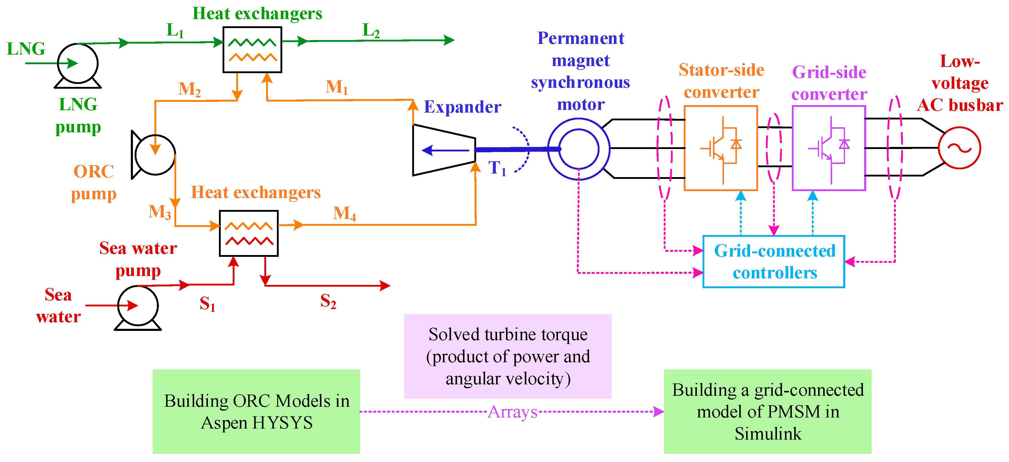
The LNG cold power generation process involves many hydrodynamic parameters and nonlinear disturbances, so it is extremely difficult to establish the most accurate analytical model. However, the heat exchanger elements of the LNG cold power generation system can be described by a low-order state model, which greatly simplifies the computational complexity. In this paper, a unipolar ORC cold energy generation structure is used, and its model topology is shown in Figure 1. L, M, and S in Figure 1 represent LNG material flow, ORC intermediate medium material flow, and seawater flow, respectively. In addition, the dashed lines represent signal acquisition; the dotted lines represent signal flow.
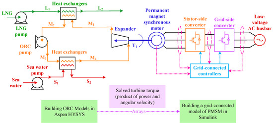
Figure 1.
Topology of unipolar ORC cold power generation structure.
2.1. Heat Exchanger Dynamic Modeling
The steady-state operation of a heat exchanger is the ability to maintain a fixed energy transfer. If the internal structure of the heat exchanger is not taken into account, the definition of the heat exchanger mass inlet thermodynamic temperature time domain expression for u(t), the outlet thermodynamic temperature time domain expression for v(t), the introduction of gain coefficient K, and the heat exchanger single-end transfer relationship is expressed as follows:
If the heat transfer function for low time scales is considered, the transient output will carry some inertia, and the change is modeled using a first-order inertial link, i.e.,
where J is the inertia coefficient, which is determined by the heat exchanger equipment parameters and work masses.
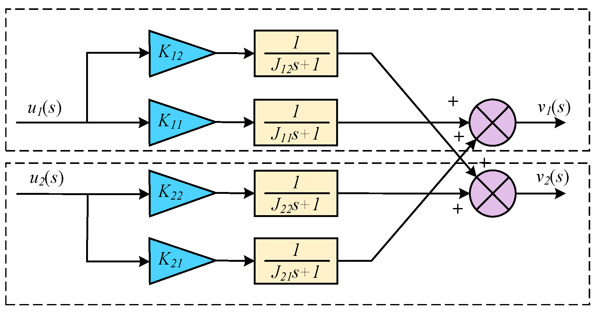
The double-ended heat exchanger has a coupling relationship, and its transfer relationship is shown in Figure 2.
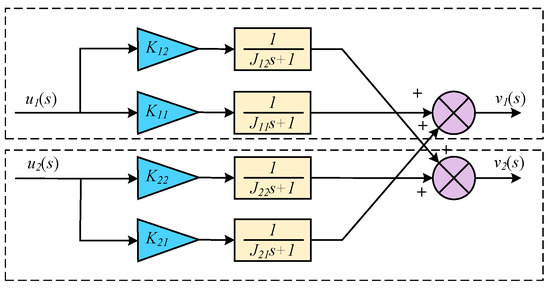
Figure 2.
Block diagram of double-ended heat exchanger coupling transfer relationship.
Where K11, K12, K21, K22 represent the proportional gain of the two-port heat exchanger; J11, J12, J21, J22 represent the inertia coefficients of the two-port heat exchanger; u1 and v1 represent the high-temperature measurement of inlet and outlet temperatures; u2 and v2 represent the low-temperature measurement of inlet and outlet temperatures, respectively.
The two-port heat exchanger transfer matrix function is expressed as follows:
According to the principle of energy conservation, the number of heat exchanger ports is extended to n and the proportional gain satisfies the constraints:
The inertia coefficients satisfy the constraints:
The mass flow rate of the work masses at each port of the heat exchanger is kept constant at steady state, and according to the principle of conservation of energy, the transferred thermal power is expressed as follows:
where ΔPt is the heat transfer power (unit: kW), the lowering of the workpiece temperature represents the radiant energy, and the heat transfer power is positive; the higher workpiece temperature represents the absorbed energy, and the heat transfer power is negative; λ1 and λ2 represent the specific heat capacity of the workpiece measured at high and low temperatures (unit: kJ·kg−1·K−1); F1 and F2 represent the mass flow rates measured at high and low temperatures (unit: kg·s−1); F1 and F2 represent the mass flow rate (unit: kg·s−1) for both high and low temperature measurements.
2.2. Equivalent Modeling of Mass Pumps and Turbines
2.2.1. Equivalent Modeling of Mass Pumps
Figure 1 contains a seawater pump, an LNG pump and an ORC pump, and the three pumps are very similar in their dynamic processes, although they have different heads and powers. This paper does not take into account the warming phenomenon generated by the internal friction of the fluid. In addition, the process of the work masses into and out of the work masses pump does not involve a phase transition. Therefore, the process of pressurization of the work masses pump is equivalent to the fluid flowing from the low-pressure side to the high-pressure side; this entropy-decreasing process can be described as a voltage source in the circuit system, and the Ppumo load of the work masses pump is obtained according to the kinetic energy formula for the work masses pump, expressed as follows:
where F is the mass flow rate; ηp represents the efficiency of the mass pump; hpi and hpo are the enthalpies of the input and output masses of the mass pump (unit: kJ/kg), respectively. The enthalpy of a medium is affected by internal energy and pressure potential. The magnitude of the enthalpy difference is influenced by the change in fluid pressure since the temperature of the medium remains constant before and after pressure application [12]. According to the enthalpy difference expression:
where Δp is the difference in mass pump pressure; ρ is the average density of the mass before and after input to the mass pump, which can be provided by the manufacturer. Therefore, the power output of the work masses pump during stable operation is proportional to the square of the mass flow rate.
2.2.2. Turbine Equivalent Model
The turbine equivalent model is similar to the worker pump model, but the turbine absorbs the kinetic energy of the worker, so this process of entropy increase can be described as a reverse electromotive force load. According to Equation (7), the turbine absorbed power is expressed as follows:
where ηt represents the turbine drive efficiency; hti and hto are the enthalpy (in kJ/kg) of the turbine input and output masses, respectively. The turbine drive shaft is directly connected to the synchronous generator, so there is no mechanical loss in this process. Then, the power absorbed by the turbine is equal to the mechanical power of the permanent magnet synchronous motor.
This is known from the mechanical torque expression:
Bring in the equation of rotation:
where Ttur is the output mechanical torque of the turbine; I is the turbine moment of inertia, given by the manufacturer; and ωt is the angular frequency of rotation of the turbine rotor shaft.
2.3. ORC Cold Energy Generation Polymerization Drive Model
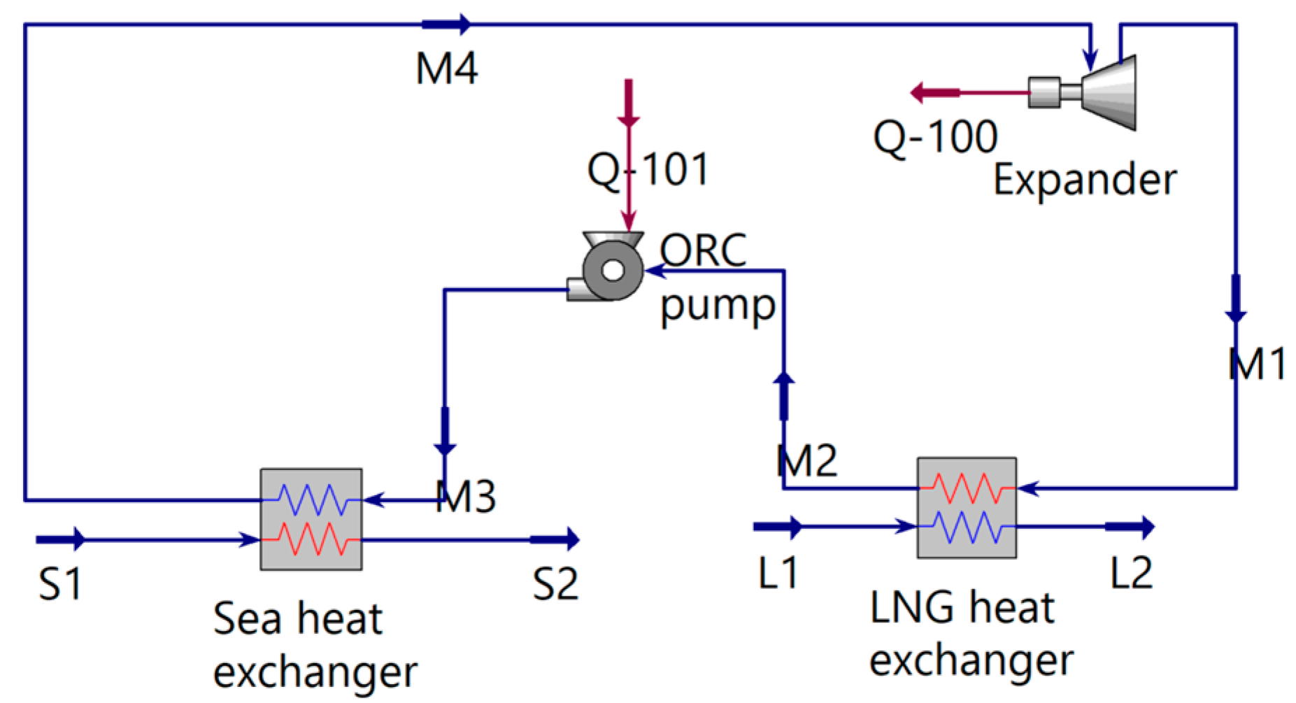
First, in order to represent the phase change process of the ORC mass, a delayed link is used to simulate the temperature change in the phase change. In addition, the turbine and the ORC pump do not generate the phase transition. Based on the component models developed in the previous two sections, they are built in Aspen HYSYS, as shown in Figure 3.
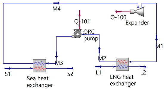
Figure 3.
Monopole ORC built in Aspen HYSYS.
Q-100 in Figure 3 is the solved mechanical load (in kW) of the turbine, which will be input into Simulink along with the turbine speed as a dataset.
According to the conservation of energy, the thermal energy in the seawater passes through the heat exchanger to make the ORC mass gasify; the kinetic energy generated by the gasification pushes the turbine to rotate and generate torque; the gaseous ORC mass passes through the heat exchanger to liquefy it while the LNG cold energy is transferred to the liquid mass. The heat exchangers in Figure 1 will correspond to the corner markers of Equation (3), respectively; the seawater–intermediate work mass heat exchanger will be labeled as SM in the lower corner; the intermediate work mass–LNG heat exchanger will be labeled as ML in the lower corner; moreover, the flow directions of the work masses for each part of the different ORC processes are defined as the corner markers of the corresponding parameters in Figure 1. Defining the Kelvin temperature 0 K as the base temperature, the thermal energy inertia state is expressed as follows:
where T represents the transfer matrix function in Equation (3). The input and output internal energies are as follows:
where I2 represents the second-order unit matrix; O2 represents the second-order zero matrix. Combining Equations (9) and (11), the ORC cold energy generation aggregation drive model can be obtained.
3. Three-Phase Permanent Magnet Synchronous Generator Model
The three-phase Permanent Magnet Synchronous Motor (PMSM) is widely used in the field of power generation, which uses permanent magnets to establish an excitation magnetic field, and it is able to eliminate the reactive power generated by the excitation current [21,22,23].
3.1. PMSM Fifth-Order Equation of State
In the previous chapter, it was learned that the turbine absorbed power is equal to the PMSM mechanical power, so the PMSM mechanical equation is expressed as follows:
where φ represents the synchronous electromechanical angle; Hp, Pe, and Dp are the PMSM inertia coefficient, electromagnetic power, and damping coefficient, respectively. Therefore, the dynamic equations for the synchronous generator rotation angle and frequency are obtained.
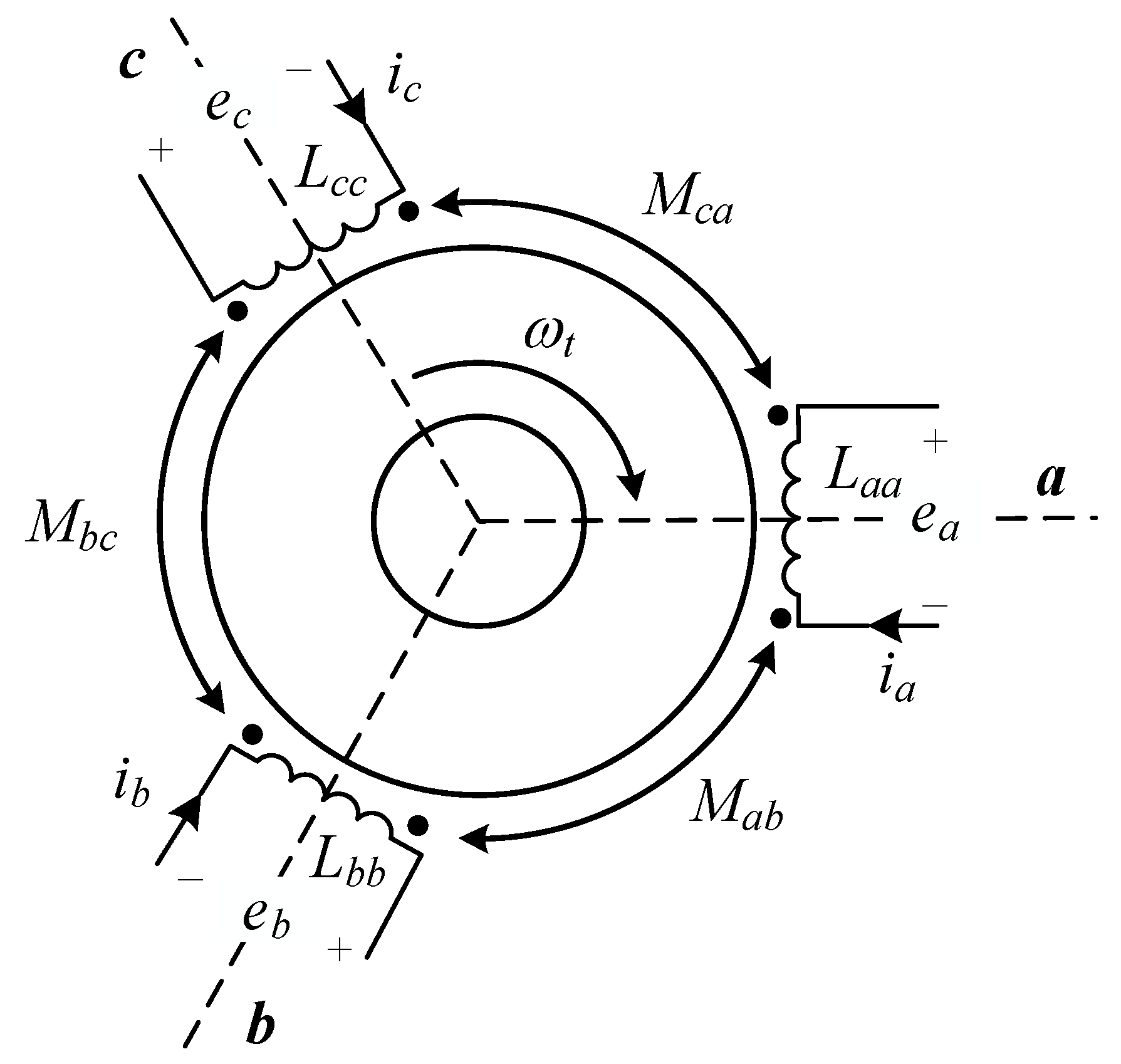
The rotor magnetic chain of the PMSM is constant, and a constant three-phase sinusoidal electromotive force is generated in the stator when the turbine has a constant torque output. Figure 4 shows the physical model of the PMSM.
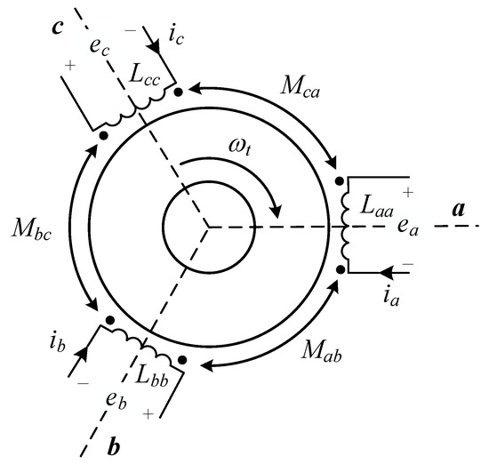
Figure 4.
PMSM physical model.
In Figure 4, Laa, Lbb, and Lcc denote the stator winding abc-phase self-inductance, respectively; Mab, Mbc, and Mca denote the stator winding mutual inductance, respectively. According to the PMSM physical model, the PMSM voltage equation and the magnetic chain equation can be known:
where Rs represents the stator internal resistance; ψf represents the permanent magnet generating magnetic chain; ea, eb, and ec represent the three-phase induced electromotive force of the PMSM generator state; and ia, ib, and ic represent the three-phase induced currents, respectively. The integration of Equations (11) and (12) is the fifth-order state equation of the PMSM.
3.2. PMSM Power Transmission Expression
The relationship between mechanical power and electromagnetic power can be obtained from the PMSM fifth-order equation of state. The actual output power expression can be obtained according to the PMSM voltage equation. The output of the synchronous generator is a three-phase non-sinusoidal alternating current (AC), which needs to be converted into electrical energy that can be connected to the AC distribution grid through a direct-drive power electronic converter device.
The power generated by the PMSM will eventually be delivered to the distribution grid, and its control method is often constant power control, so the PMSM will maintain constant power output during stable operation. Let the PMSM output power be Ppm. According to the voltage balance equation, the synchronous machine output power can be expressed as follows:
If the grid-connected power output is kept constant, then Ppm is a constant value, and if the input mechanical power to the turbine is not sufficient to meet the grid-connected output power requirement, then it will lead to a decrease in the induced electromotive force of the synchronous machine, which will result in damage to the power electronics. To protect the grid-connected system, this accident can be avoided by introducing feedback control.
4. Direct-Drive Electrical Drive Analysis
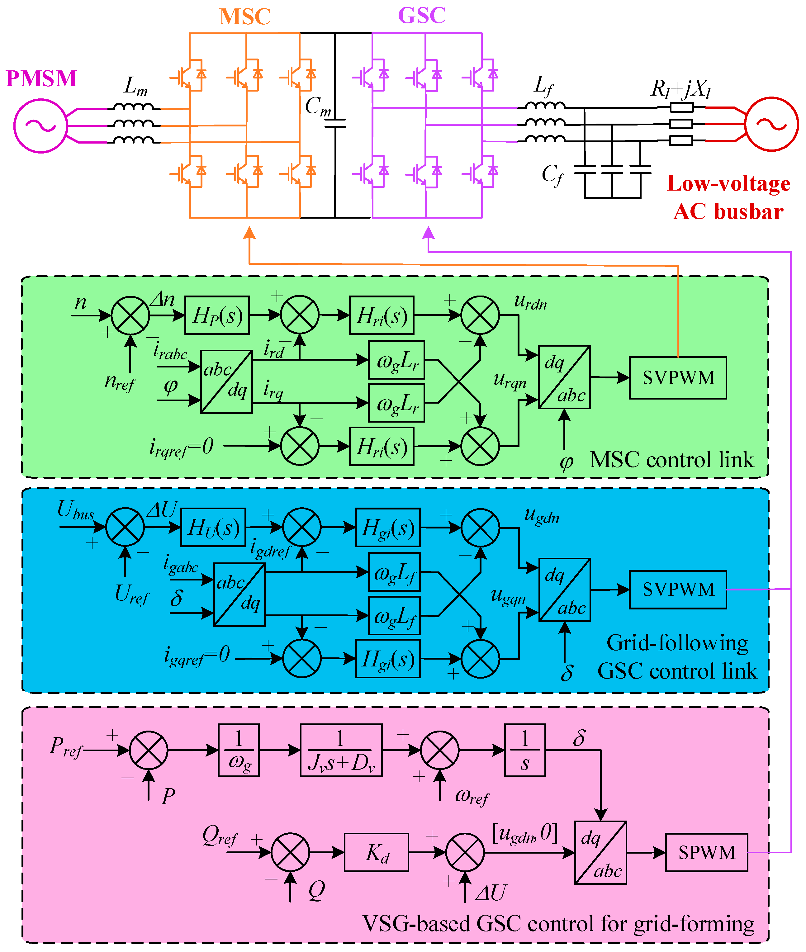
The direct-drive electrical drive structure is commonly used in the wind turbine grid-connected drive structure, which is an AC-DC-AC electrical drive composed of the machine-side converter (MSC) and the grid-side converter (GSC) [24]. A three-phase two-level bridge full-control circuit is used as the power electronic topology of the machine-side and grid-side converters, and its circuit topology and control block diagram are shown in Figure 5.
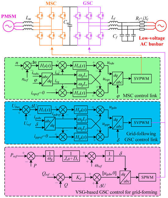
Figure 5.
Direct-drive electric drive circuit topology and control link block diagram.
In the main circuit of Figure 5, Lm represents the boost inductor; Cm represents the DC bus filter capacitance; Lf and Cf represent the inductance and capacitance of the low-pass filter, respectively; Rl and Xl represent the line equivalent resistance and reactance, respectively. In the control link of Figure 5, the subscript abc represents the three-phase synchronous coordinate system, the subscript dq represents the orthogonal rotating coordinate system, and the subscript n represents the signal waveform of the switching device; H(s) denotes the transfer function of the proportional–integral link; ir and ig represent the stator-side current and the grid-side output current, respectively; the parameters Jv and Dv are inertia coefficients and damping coefficients, respectively, and kd represents the reactive power–voltage droop coefficient, with a virtual synchronous generator (VSG) as an example to illustrate the grid-forming control method.
4.1. Expression of the Electrical Drive of a Grid-Side Converter with Constant Power Control
GSC is used to convert the DC power generated by the machine-side converter into AC power that can be connected to the distribution grid. Due to the different expressions of electrical transmission caused by the different power control methods, its grid-connected power control methods are mainly categorized into two types: grid-following-type grid-connected control and grid-constructing-type grid-connected control [25,26].
4.1.1. Grid-Following-Type Grid-Connected Control Method
The follow-the-grid type of grid-connected control method collects the real-time frequency of the grid through a phase-locked loop (PLL) and generates current through the potential difference between the inverter and the grid [27,28]. The grid-connected current value is directly related to the line impedance. The LPF equivalent impedance value is first integrated into the line impedance:
where ωg is the grid angular frequency. LPF devices are often selected to satisfy . Therefore, the impedance integration value is simplified as follows:
The grid-following-type constant power grid-connected control is implemented by voltage vector control, current-based virtual synchronous generator, etc. In this paper, the voltage vector control method is used to implement the power control. Therefore, the output power of the grid-control of the grid-following type is expressed as follows:
where Eg represents the grid voltage RMS; Ev represents the inverter synchronization voltage RMS. The inverter power angle is synchronized with the grid, so the reactive power is absorbed by the line reactance.
4.1.2. Grid-Forming Grid-Connected Control Method
The grid-forming grid-connected control method is used to generate the virtual power angle from the difference between the active power reference value and the active power collection value, which in turn creates a phase angle difference with the line impedance power angle and the grid power angle, and thus realizes the current delivery. The virtual synchronous generator power angle is generated by its VSG δ to satisfy the synchronous machine power angle equation [29,30,31,32]:
where ωv is the angular frequency generated by the VSG; Pref and ωref are the reference active power, respectively; Hv and Dv are the virtual inertia coefficient and damping coefficient, respectively. Therefore, assuming that the grid power angle is θ, the power expression of the constructive grid-type grid-connected control method is deduced as follows [33]:
4.2. GSC, MSC Drive Mode
The previous subsection derived the power expressions for the grid-following-type control and the grid-forming-type control, and in this section the average equivalent model of the direct-drive structure will be derived, which can be used as a reference for the optimal scheduling modeling. The electrical drive expression of the converter based on the average equivalent model is derived by considering the power output as a self-sustained load with fixed power.
4.2.1. Mean Value Relationship for MSC
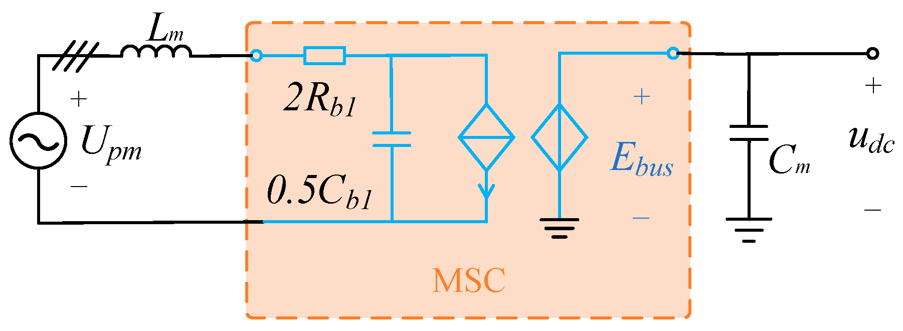
The role of the MSC is to convert the AC electrical energy generated by the PMSM into DC regulated electrical energy. The topology shown in Figure 5 is a boosted three-phase fully controlled rectifier circuit with the input side average equivalent model modeled as a controlled current source with the maximum value of the AC as reference. The output side average equivalent model takes the DC voltage as the reference and models it as a controlled voltage source. The average equivalent circuit model of the three-phase fully controlled rectifier circuit is shown in Figure 6.
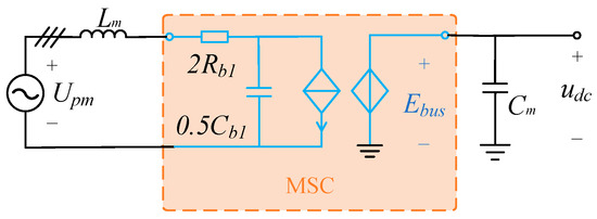
Figure 6.
Average equivalent circuit diagram for MSC.
In Figure 6, Rb1 and Cb1 represent the switching tube on-resistance and junction capacitance, respectively. Because of the pulse width modulation rectifier using a two-level fully controlled circuit, two sets of switching tubes are used for each onset of the generated current, which puts two sets of Rb1 and Cb1 in series, and thus a correction factor exists.
The controlled signals in the average equivalent circuit of the MSC come from the control circuit, and the control of the MSC power electronics consists of proportional–integral control. In addition, the synchronization frequency of the PMSM is captured by the PLL, and its specific control process is similar to that of the PLL of the grid-following type grid-connected control method, which will not be discussed in this paper.
4.2.2. Grid-Side Converter Drive Mode
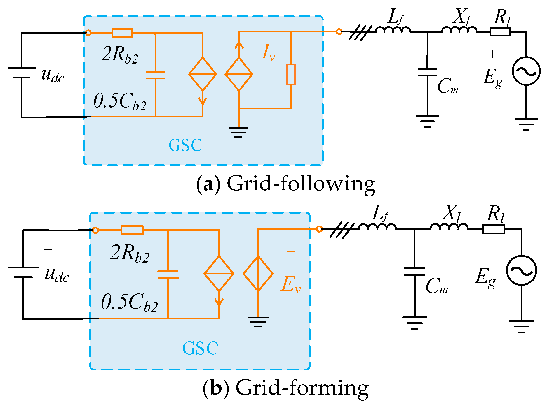
The GSC takes the DC output from the MSC and delivers current to the grid according to the constant power control method in the previous section. The design principle of the average equivalent model of the GSC is similar to that of the average equivalent model of the MSC. The average equivalent circuit model of the GSC for the grid-following and grid-forming types is shown in Figure 7.
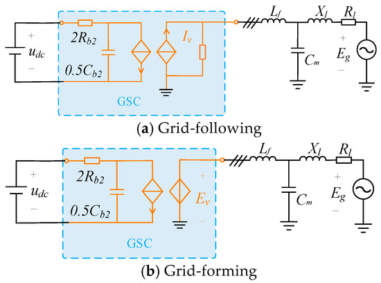
Figure 7.
Average equivalent circuit diagrams of the GSC for the grid-following and grid-forming drives.
In Figure 7, Rb2 and Cb2 represent the switching tube conduction resistance and junction capacitance, respectively.
According to the constant power control output value, the GSC output can be equated to a resistive load that absorbs active power at a constant rate. In addition, the GSC junction capacitance does not absorb active power, so ignoring the junction capacitance yields the active power transmission of the DC bus, expressed as follows:
The DC bus filter capacitors also do not absorb a large amount of active power, so the active power of the synchronous machine load is expressed as follows:
where Upm is the RMS value of the three-phase induced electromotive force of the PMSM.
5. Simulation Verification
In this paper, a grid-connected drive model for LNG cold power generation is proposed to first verify the heat transfer performance of the ORC link. The ORC work masses are defined as propane in HYSYS [4], and after solving the model it is possible to determine the complete ORC output mechanical power and LNG temperature rise.
5.1. Validation of ORC Internal Energy Relations
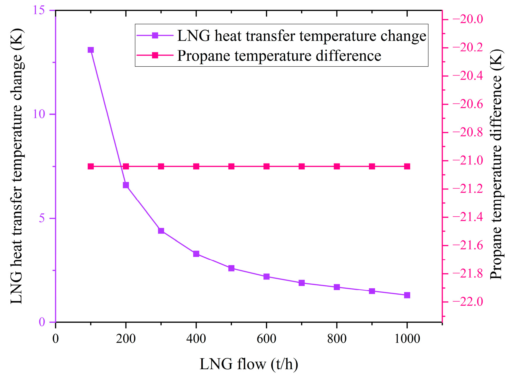
Cold energy generation is a part of realizing LNG cold energy cascade utilization, and the ORC topology is built according to Figure 1. In this paper, the input power of the ORC pump is defined as a constant 3 kW, so that it produces a constant pressure difference [34]; according to the relevant data from the Caofeidian LNG station in China, the heat exchanger has an LNG inlet temperature of −172 °C and a pressure of 730 kPa. Due to the conservation of energy, the total energy of the ORC system does not change, and therefore the steady state parameters within the system are linear. The LNG flow rate through the heat exchanger is first varied, and the LNG temperature difference and propane temperature difference are observed. The relationship between LNG flow rate and LNG temperature difference and propane temperature difference is shown in Figure 8.
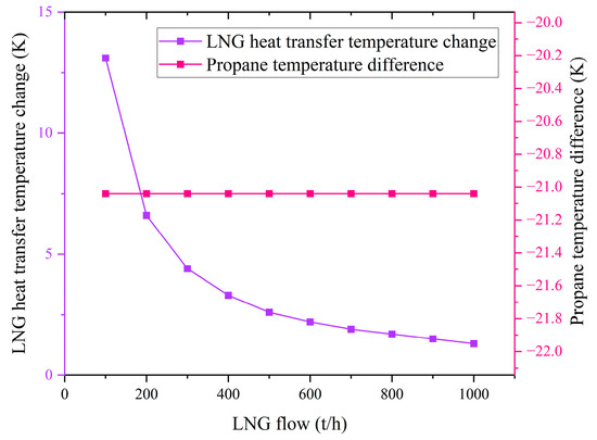
Figure 8.
Relationship between LNG flow rate and heat transfer temperature difference.
It can be seen in Figure 8 that the temperature difference in propane does not change, and this is because the turbine pressure difference is constant, making the ORC output energy remain constant. The LNG heat transfer temperature difference is directly proportional to its energy, while the square of the flow rate is directly proportional to its energy, so the plot of LNG flow rate versus the LNG temperature difference is in the shape of a parabola. In addition, the experiment was repeated by varying the ORC flow rate and the results are shown in Figure 9.
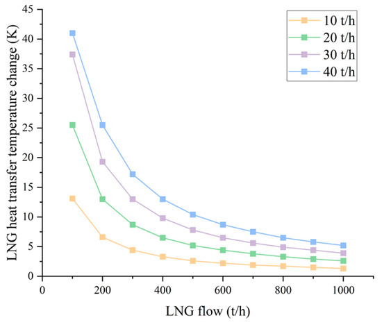
Figure 9.
Effect of propane flow rate on LNG temperature difference.
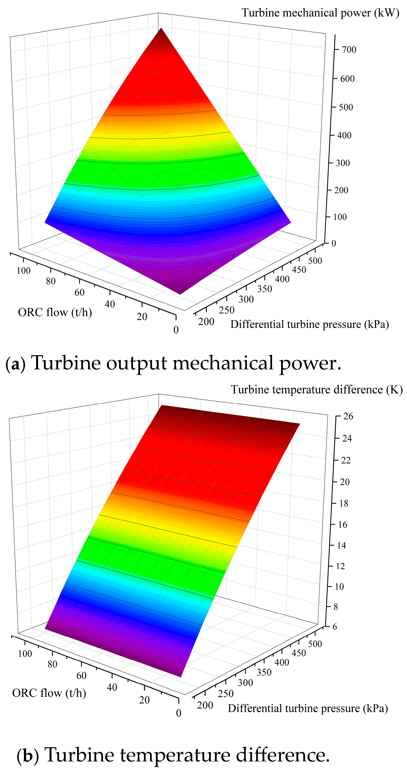
In Figure 9, it can be seen that the heat absorbed by the LNG increases when the propane flow rate increases, which is because the increase in propane flow rate increases the output mechanical power of the turbine. The turbine mechanical power is determined by the flow rate and pressure difference together, but the propane gas density is affected by the temperature and pressure, so the mapping relationship of the output mechanical power is established by the simulation data. Figure 10a shows the mapping relationship between the mechanical power of the turbine and the propane flow rate and pressure difference; Figure 10b shows the mapping relationship between the temperature difference in the turbine and the propane flow rate and pressure difference.

Figure 10.
Mechanical power and temperature difference with differential pressure and ORC flow.
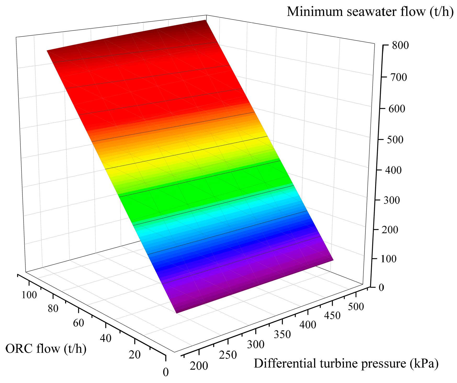
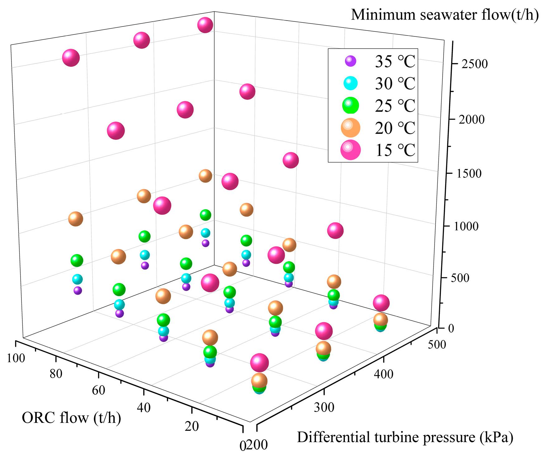
In Figure 10a, it can be seen that the mechanical power output increases when the turbine pressure difference and ORC flow rate increase together, but this also increases the burden of the seawater pump. In Figure 10b, it can be seen that the turbine temperature difference is linearly related to the turbine pressure difference and ORC flow rate. In addition, in order to study the relationship between the required seawater flow rate and the turbine pressure difference and ORC flow rate, the mapping relationship is obtained by solving the problem. The parameters at the LNG end are fixed, and it is ensured that the seawater cannot freeze during the heat transfer process, so Figure 11 shows the relationship between the minimum seawater flow rate and the pressure difference, and ORC flow rate when the seawater input temperature is kept at 25 °C. Figure 12 is a scatter plot of the minimum seawater flow rate required for different seawater input temperatures.

Figure 11.
Minimum seawater flow versus differential pressure, ORC flow.
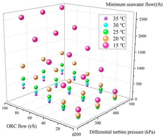
Figure 12.
Comparison of different seawater input temperatures.
The figure shows that the minimum seawater flow rate has a linear relationship with the turbine pressure difference and ORC flow rate, and at the same time the lower the seawater input temperature, the greater the amount of seawater consumed. However, a phase change occurs when the seawater input temperature is too low, which affects the safety of the system operation.
5.2. Verification of Direct-Drive Driveline
Based on the ORC output mechanical power as the input of the direct-drive system, the defined PMSM and main circuit parameters are shown in Table 1, and the related control parameters are shown in Table 2. In this paper, vector control and VSG control are used to form the carrier, and space vector pulse width modulation is used to form the switching tube control signal.

Table 1.
PMSM basic parameters.
Table 2.
Control link parameters.
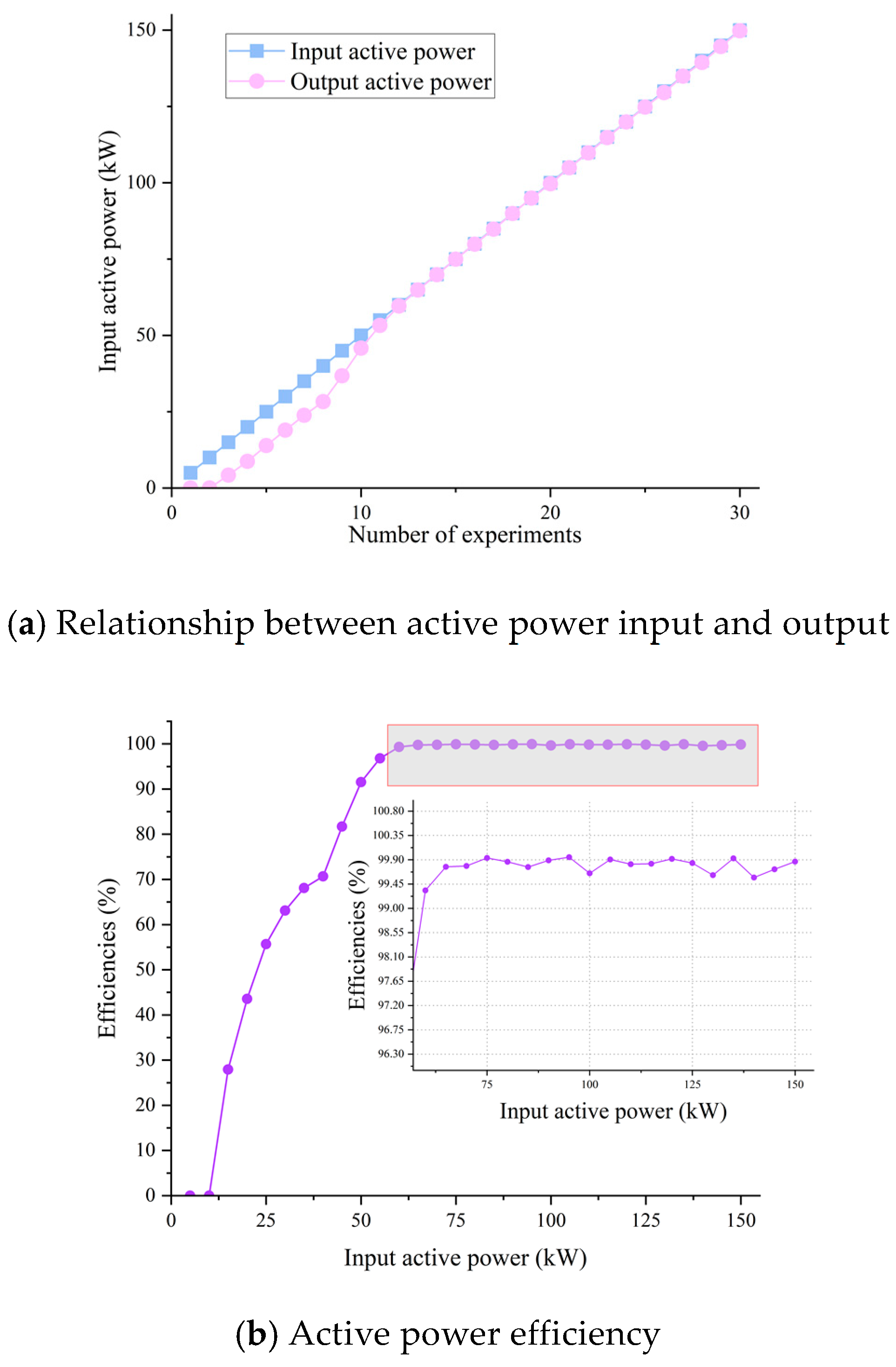
Based on the parameters above, the direct-drive grid-connected system of PMSM was built in Simulink, and firstly, the active power input and output relationship and its drive efficiency were verified, and we chose a 690 V low-voltage AC bus as the grid-connected end. The experiment started at the input power of 5 kW and increased 5 kW for each experiment, stopping at 500 kW. We found that the energy transmission efficiency changes less as the number of experiments increases. Thus, Figure 13 shows the comparison of energy relations for power input from 5 kW to 150 kW.

Figure 13.
Active power relations and efficiency relations for direct-drive drive systems.
According to Figure 13a, it can be seen that the output power is 0 when the input power is less than 10 kW, and this is because at this time the torque is too small to drag the rotor to rotate. Observing Figure 13b, it can be seen that the rotor moves when the input power is more than 15 kW and the efficiency increases with the increase in input power. The efficiency stabilizes above 99% when the input power reaches 65 kW, and the losses mainly come from the PMSM stator copper losses, iron losses, and the switching losses and pass-state losses of the switching devices.
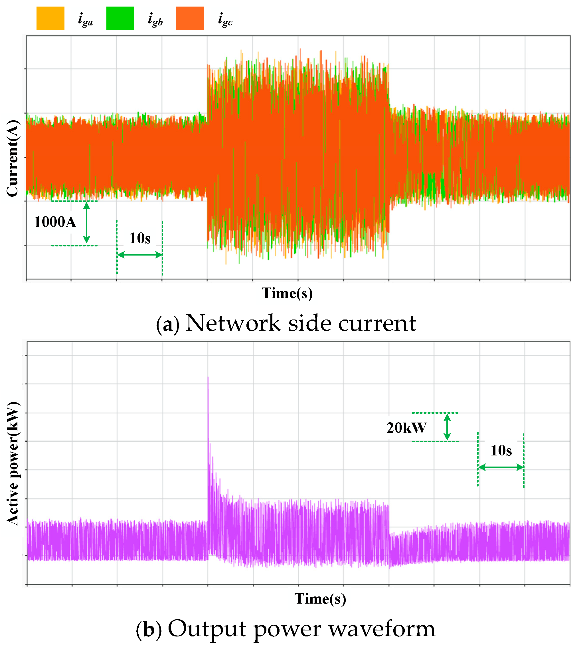
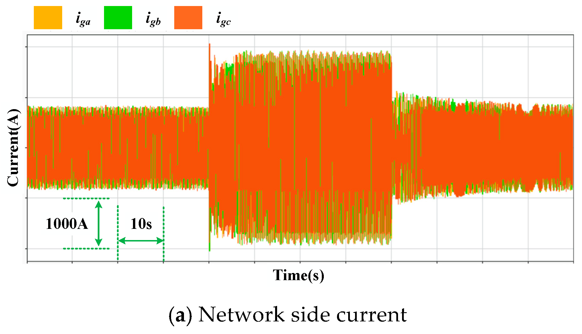
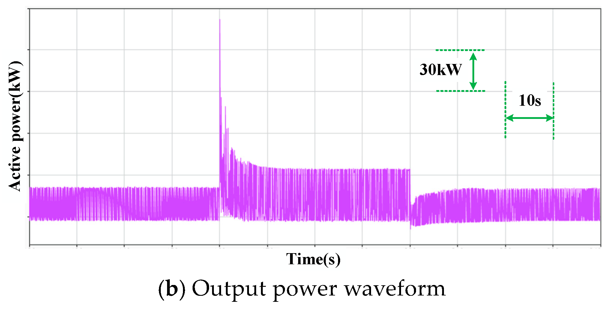
In addition, comparing the response of the grid-follow type and the grid-forming type when the output power of the turbine is changed, we assume that the ORC work-masses flow rate increases or decreases for some reason, which makes the mechanical power output of the turbine change. The steady state output power is 50 kW, and the mechanical power is increased to 100 kW for 40 s, after which the output power is returned to 50 kW. The output active power and current waveforms are observed for the grid-following-type control scheme and the grid-forming-type control scheme, respectively, as shown in Figure 14 and Figure 15.

Figure 14.
Current and active power output for grid-following type control.

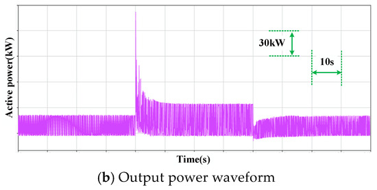
Figure 15.
Current and active power output for grid-forming type control.
In Figure 14 and Figure 15, we can see that both the grid-following control method and the grid-forming control method are able to realize the power transfer. Similarly, the same conclusion can be obtained by trying larger power inputs.
Considering the experiments as above, Refs. [11,12,13,14,15,16,17] will be compared to the method of this paper, as shown in Table 3.
Table 3.
Summary of model comparisons.
6. Conclusions
Cold power generation is a part of LNG cold energy utilization, but the mathematical description of LNG cold energy to AC grids is lacking in existing studies. In order to fill the gap here, this paper adopts the unipolar Rankine cycle of cold energy to mechanical energy transmission method and establishes the corresponding model; it designs the direct-drive grid-connected structure of permanent magnet synchronous motor and constructs the energy transfer model from mechanical energy to electric energy. The details are summarized as follows:
- (1)
- We constructed a higher-order thermodynamic model for the unipolar ORC. Based on the first-order heat transfer equation, a two-port heat exchanger model is constructed. We constructed ORC aggregated drive equations by integrating the turbine and pressurized pump energy input–output relationship.
- (2)
- Mathematical expressions of induced electric angle, induced electric potential, and induced current were obtained based on the fifth-order equation of state of permanent magnet synchronous generator.
- (3)
- We studied the direct-drive grid-connected structure of PMSM to establish the average equivalent model of motor-side and grid-side power electronic converters. In addition, the power expressions for the grid-following and grid-forming types of control were analyzed separately.
- (4)
- Finally, we verified the influencing factors of the turbine output in the ORC process and the required minimum seawater flow through Aspen HYSYS. A grid-connected model of a PMSM direct-drive connected to a low-voltage AC bus was constructed through Simulink to examine the transfer efficiency as well as the time-domain waveforms of the system.
Author Contributions
Conceptualization, Y.Q.; methodology, Y.Q.; validation, Y.G.; formal analysis, P.Z.; investigation, Y.Q.; writing—original draft preparation, Y.Q.; writing—review and editing, Y.G.; visualization, D.W. and Y.G.; project administration, D.W. and R.L.; funding acquisition, P.Z. All authors have read and agreed to the published version of the manuscript.
Funding
This work was funded by S&T Program of Hebei (242Q4052Z); Overseas Expertise Introduction Project of Hebei (2023YX044A).
Data Availability Statement
The data that support the findings of this study are available from the First author, [Yu Qi], upon reasonable request.
Conflicts of Interest
No potential conflicts of interest were reported by the authors with Caofeidian Xintian LNG Co., Ltd.
References
- Pan, J.; Cao, Q.; Li, M.; Li, R.; Tang, L.; Bai, J. Energy integration of light hydrocarbon separation, LNG cold energy power generation, and BOG combustion: Thermo-economic optimization and analysis. Appl. Energy 2024, 356, 122450. [Google Scholar] [CrossRef]
- Kanbur, B.B.; Xiang, L.; Dubey, S.; Choo, F.H.; Duan, F. Cold utilization systems of LNG: A review. Renew. Sustain. Energy Rev. 2017, 79, 1171–1188. [Google Scholar] [CrossRef]
- Cheng, H.; Ju, Y.; Fu, Y. Thermal performance calculation with heat transfer correlations and numerical simulation analysis for typical LNG open rack vaporizer. Appl. Therm. Eng. Des. Process. Equip. Econ. 2019, 149, 1069–1079. [Google Scholar] [CrossRef]
- He, T.; Chong, Z.R.; Zheng, J.; Ju, Y.; Linga, P. LNG Cold Energy Utilization: Prospects and Challenges. Energy 2019, 170, 557–568. [Google Scholar] [CrossRef]
- Joy, J.; Chowdhury, K. Appropriate number of stages of an ORC driven by LNG cold energy to produce acceptable power with reasonable surface area of heat exchangers. Cryogenics 2022, 128, 103599. [Google Scholar] [CrossRef]
- Zheng, X.; Li, Y.; Zhang, J.; Zhang, Z.; Guo, C.; Mei, N. Design and multi-objective optimization of combined air separation and ORC system for harnessing LNG cold energy considering variable regasification rates. Int. J. Hydrogen Energy 2024, 57, 210–223. [Google Scholar] [CrossRef]
- Cao, Y.; Wang, J.; Li, Y.; Deng, H.; Fu, W. Thermodynamic performance analysis of a novel integrated energy cascade system of liquid air energy storage and two-stage organic Rankine cycles. J. Energy Storage 2024, 75, 109687. [Google Scholar] [CrossRef]
- Lu, Y.; Xu, J.; Chen, X.; Tian, Y.; Zhang, H. Design and thermodynamic analysis of an advanced liquid air energy storage system coupled with LNG cold energy, ORCs and natural resources. Energy 2023, 275, 127538. [Google Scholar] [CrossRef]
- Mehrpooya, M.; Sharifzadeh, M.M.M.; Katooli, M.H. Thermodynamic analysis of integrated LNG regasification process configurations. Prog. Energy Combust. Sci. 2018, 69, 1–27. [Google Scholar] [CrossRef]
- Bao, J.; Yuan, T.; Zhang, L.; Zhang, N.; Zhang, X.; He, G. Comparative study of liquefied natural gas (LNG) cold energy power generation systems in series and parallel. Energy Convers. Manag. 2019, 184, 107–126. [Google Scholar] [CrossRef]
- Ma, J.; Song, X.; Zhang, B.; Mao, N.; He, T. Optimal design of dual-stage combined cycles to recover LNG cold energy and low-temperature waste thermal energy for sustainable power generation. Energy Convers. Manag. 2022, 269, 116141. [Google Scholar] [CrossRef]
- Sun, Z.; Lai, J.; Wang, S.; Wang, T. Thermodynamic optimization and comparative study of different ORC configurations utilizing the exergies of LNG and low grade heat of different temperatures. Energy 2018, 147, 688–700. [Google Scholar] [CrossRef]
- Zhao, Y.; Hu, D.; Cai, D.; Wang, Y.; Liang, Y. Study on strengthening power generation by using LNG cold energy with multi-stream heat exchange. Appl. Therm. Eng. 2023, 234, 121262. [Google Scholar] [CrossRef]
- Chitgar, N.; Hemmati, A.; Sadrzadeh, M. A comparative performance analysis, working fluid selection, and machine learning optimization of ORC systems driven by geothermal energy. Energy Convers. Manag. 2023, 286, 117072. [Google Scholar] [CrossRef]
- Fang, Z.; Shang, L.; Pan, Z.; Yao, X.; Ma, G.; Zhang, Z. Exergoeconomic analysis and optimization of a combined cooling, heating and power system based on organic Rankine and Kalina cycles using liquified natural gas cold energy. Energy Convers. Manag. 2021, 238, 114148. [Google Scholar] [CrossRef]
- Li, C.; Liu, J.; Zheng, S. Performance analysis of an improved power generation system utilizing the cold energy of LNG and solar energy. Appl. Therm. Eng. 2019, 159, 113937. [Google Scholar] [CrossRef]
- Cui, X.; Chen, X.; Gao, Z. Research on the power generation performance and optimization of thermoelectric generators for recycling remaining cold energy. Energy 2024, 299, 131422. [Google Scholar] [CrossRef]
- Hu, X.; Zhang, S.; Tang, S.; Peng, Z. Dynamic Modeling of Energy Flow in Heat Supply Network Considering Working Fluid and Heat Conduction. Proc. CSEE 2021, 41, 4198–4208. [Google Scholar]
- Shen, X.; Liu, J.; Lin, H.; Yin, Y.; Alcaide, A.M.; Leon, J.I. Cascade Control of Grid-Connected NPC Converters via Sliding Mode Technique. IEEE Trans. Energy Convers. 2023, 38, 1491–1500. [Google Scholar] [CrossRef]
- Zheng, Z.; Shen, C.; Yan, J.; Yuan, M.; Liu, Y.; Fan, H. Mechanism Analysis of Oscillations Induced by Control Coupling of Voltage Source Converters in Wind Farms with Direct-driven Turbines. Autom. Electr. Power Syst. 2023, 47, 14–26. [Google Scholar]
- Jing, R.; Wang, G.; Zhang, G.; Xu, D. Review of Field Weakening Control Strategies of Permanent Magnet Synchronous Motors. CES Trans. Electr. Mach. Syst. 2024, 8, 319–331. [Google Scholar] [CrossRef]
- Wang, S.; Wang, H.; Tang, C.; Li, J.; Liang, D.; Qu, Y. Research on Control Strategy of Permanent Magnet Synchronous Motor Based on Fast Terminal Super-Twisting Sliding Mode Observer. IEEE Access 2024, 12, 141905–141915. [Google Scholar] [CrossRef]
- Song, Z.; Zhou, W. PMSM Disturbance Resistant Adaptive Fast Super-Twisting Algorithm Speed Control Method. IEEE Access 2024, 12, 138155–138165. [Google Scholar] [CrossRef]
- Stallmann, F.; Mertens, A. Sequence impedance modeling of the matching control and comparison with virtual synchronous generator. In Proceedings of the 2020 IEEE 11th International Symposium on Power Electronics for Distributed Generation Systems (PEDG), Dubrovnik, Croatia, 28 September–1 October 2020; pp. 421–428. [Google Scholar]
- Sun, P.; Xu, H.; Yao, J.; Chi, Y.; Huang, S.; Cao, J. Dynamic Interaction Analysis and Damping Control Strategy of Hybrid System with Grid-Forming and Grid-Following Control Modes. IEEE Trans. Energy Convers. 2023, 38, 1639–1649. [Google Scholar] [CrossRef]
- Lei, J.; Xiang, X.; Liu, B.; Li, W.; He, X. Quantitative and Intuitive VSG Transient Analysis with the Concept of Damping Area Approximation. IEEE Trans. Smart Grid 2023, 14, 2477–2480. [Google Scholar] [CrossRef]
- Mahmoud, K.; Astero, P.; Peltoniemi, P.; Lehtonen, M. Promising grid-forming VSC control schemes toward sustainable power systems: Comprehensive review and perspectives. IEEE Access 2022, 10, 130024–130039. [Google Scholar] [CrossRef]
- Chi, Y.; Jiang, B.; Hu, J.; Liu, W.; Liu, H.; Fan, Y.; Ma, S.; Yao, J. Grid-forming Converters: Physical Mechanism and Characteristics. High Volt. Eng. 2024, 50, 590–604. [Google Scholar]
- Bevrani, H.; Ise, T.; Miura, Y. Virtual synchronous generators: A survey and new perspectives. Int. J. Electr. Power Energy Syst. 2014, 54, 244–254. [Google Scholar] [CrossRef]
- Verma, P.; Seethalekshmi, K.; Dwivedi, B. A Self-Regulating Virtual Synchronous Generator Control of Doubly Fed Induction Generator-Wind Farms. IEEE Can. J. Electr. Comput. Eng. 2023, 46, 35–43. [Google Scholar] [CrossRef]
- Zhou, X.; Cheng, S.; Wu, X.; Rao, X. Influence of Photovoltaic Power Plants Based on VSG Technology on Low Frequency Oscillation of Multi-Machine Power Systems. IEEE Trans. Power Deliv. 2022, 37, 5376–5384. [Google Scholar] [CrossRef]
- Fu, S.; Sun, Y.; Lin, J.; Chen, S.; Su, M. P/Q-ω/V Admittance Modeling and Oscillation Analysis for Multi-VSG Grid-Connected System. IEEE Trans. Power Syst. 2023, 38, 5849–5859. [Google Scholar] [CrossRef]
- Zhang, C.; Dou, X.; He, G.; Yang, D. Cooperative robust operation control method of multi-VSG available for low- and medium-voltage distribution network. Electr. Power Autom. Equip. 2020, 40, 64–76. [Google Scholar]
- Bao, J.; Lin, Y.; Zhang, R.; Zhang, N.; He, G. Strengthening power generation efficiency utilizing liquefied natural gas cold energy by a novel two-stage condensation Rankine cycle (TCRC) system. Energy Convers. Manag. 2017, 143, 312–325. [Google Scholar] [CrossRef]
- He, T.; Ma, H.; Ma, J.; Mao, N.; Liu, Z. Effects of cooling and heating sources properties and working fluid selection on cryogenic organic Rankine cycle for LNG cold energy utilization. Energy Convers. Manag. 2021, 247, 114706. [Google Scholar] [CrossRef]
- Abbasi, H.R.; Pourrahmani, H.; Chitgar, N.; Van Herle, J. Thermodynamic analysis of a tri-generation system using SOFC and HDH desalination unit. Int. J. Hydrogen Energy 2024, 72, 1204–1215. [Google Scholar] [CrossRef]
- Kotas, T.J. Exergy criteria of performance for thermal plant: Second of two papers on exergy techniques in thermal plant analysis. Int. J. Heat Fluid Flow 1980, 2, 147–163. [Google Scholar] [CrossRef]
- Marmolejo-Correa, D.; Gundersen, T. A comparison of exergy efficiency definitions with focus on low temperature processes. Energy 2012, 44, 477–489. [Google Scholar] [CrossRef]
- Chen, W.; Lin, Y.; Luo, D.; Jin, L.; Hoang, A.T.; Saw, L.H.; Nižetić, S. Effects of material doping on the performance of thermoelectric generator with/without equal segments. Appl. Energy 2023, 350, 121709. [Google Scholar] [CrossRef]
- Chen, J.; Liao, Y.; Zhou, Q.; Liang, J.; Miao, L.; Zhu, Y.; Wang, S.; He, W.; Nishiate, H.; Lee, C.-H.; et al. Realizing high conversion efficiency in shallow cryogenic thermoelectric module based on n-type BiSb and p-type MgAgSb materials. Mater. Today Phys. 2022, 28, 100855. [Google Scholar] [CrossRef]

Disclaimer/Publisher’s Note: The statements, opinions and data contained in all publications are solely those of the individual author(s) and contributor(s) and not of MDPI and/or the editor(s). MDPI and/or the editor(s) disclaim responsibility for any injury to people or property resulting from any ideas, methods, instructions or products referred to in the content. |
© 2024 by the authors. Licensee MDPI, Basel, Switzerland. This article is an open access article distributed under the terms and conditions of the Creative Commons Attribution (CC BY) license (https://creativecommons.org/licenses/by/4.0/).