
Adaptive Variable Universe Fuzzy Droop Control Based on a Novel Multi-Strategy Harris Hawk Optimization Algorithm for a Direct Current Microgrid with Hybrid Energy Storage


Abstract
1. Introduction
- To achieve an optimal distribution of power fluctuations with varying frequency characteristics among HESS units, this study enhances droop control through variable universe fuzzy control and real-time optimization of the droop coefficient. The battery appropriately compensates for low-frequency power shortages, while the super-capacitor effectively addresses high-frequency power shortages. This approach eliminates the adverse effects of internal factors like load mutations and line impedance on power distribution, thereby ensuring the safe and stable operation of the system.
- A new MHHO is proposed by introducing Fuch mapping in the population initialization. In the exploration and exploitation phase, the golden sine strategy is introduced and a new elitism lens imaging opposition-based learning strategy is designed to improve the convergence ability of the HHO algorithm. The CEC2017 test function is compared with five new meta-heuristic algorithms to verify the excellent numerical performance of the proposed algorithm.
- The droop control of hybrid energy storage based on adaptive variable universe fuzzy logic algorithm has not been reported in previous work. By integrating the effective search capability of the MHHO algorithm with the dynamic adjustment ability of variable universe fuzzy control to the droop curve, an adaptive variable universe fuzzy droop control based on MHHO is developed. This control system adjusts the droop coefficient adaptively to mitigate the impact of line impedance on power distribution and enhance the precision of power sharing.
- Simulation and experimental results verify the correctness and effectiveness of the proposed method.
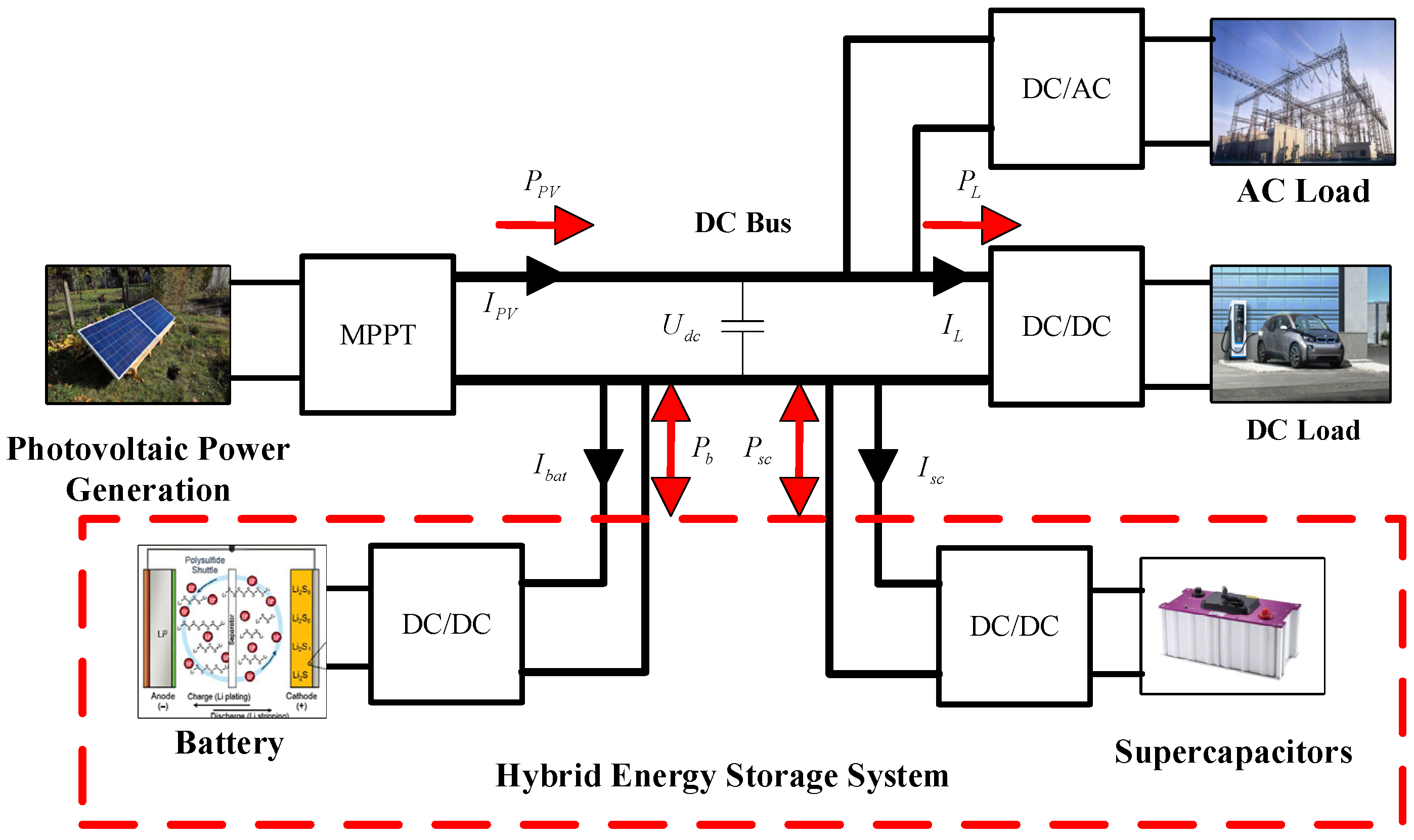
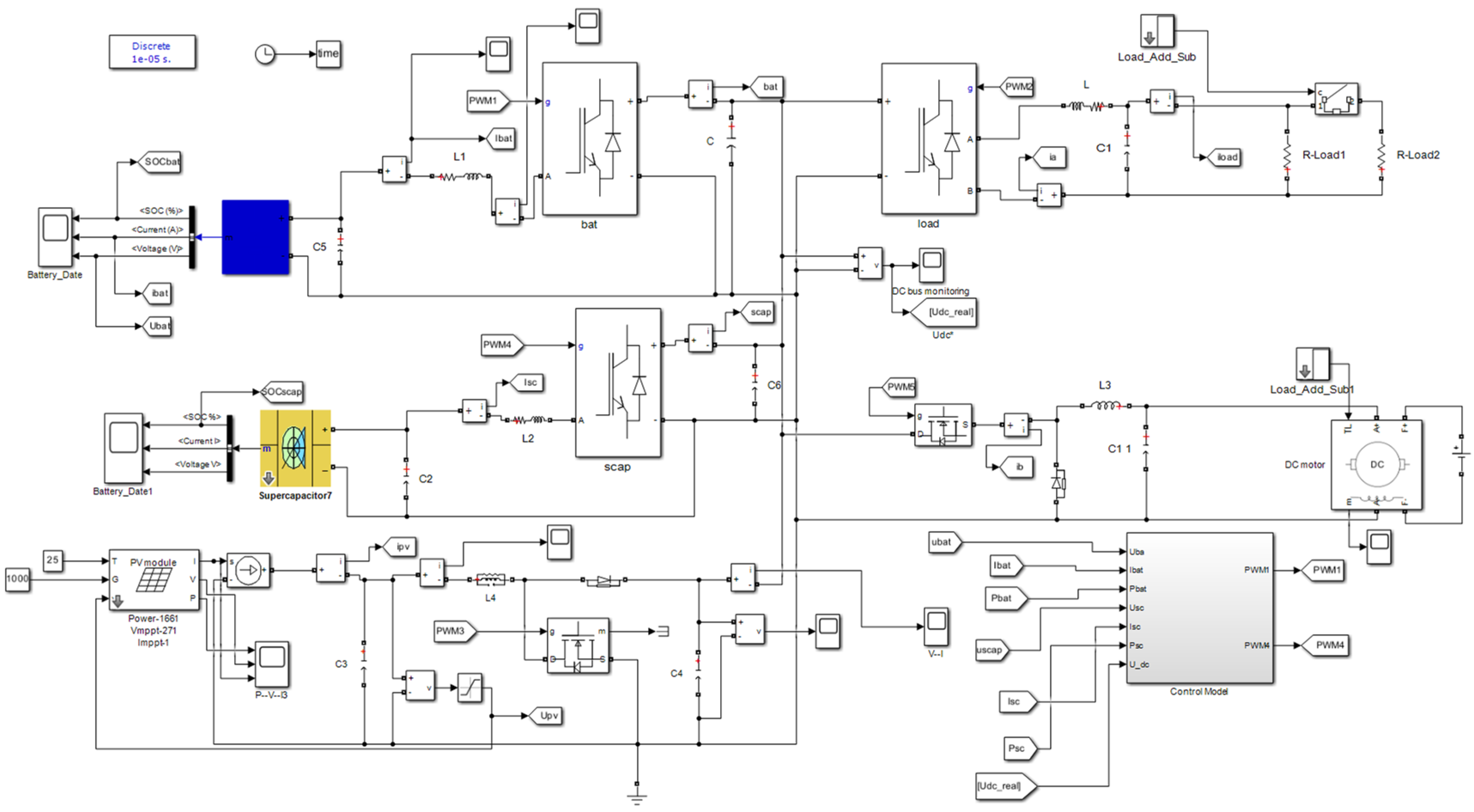
2. Photovoltaic DC Microgrid System Structure
2.1. System Structure
2.2. Topological Structure of Main Circuit
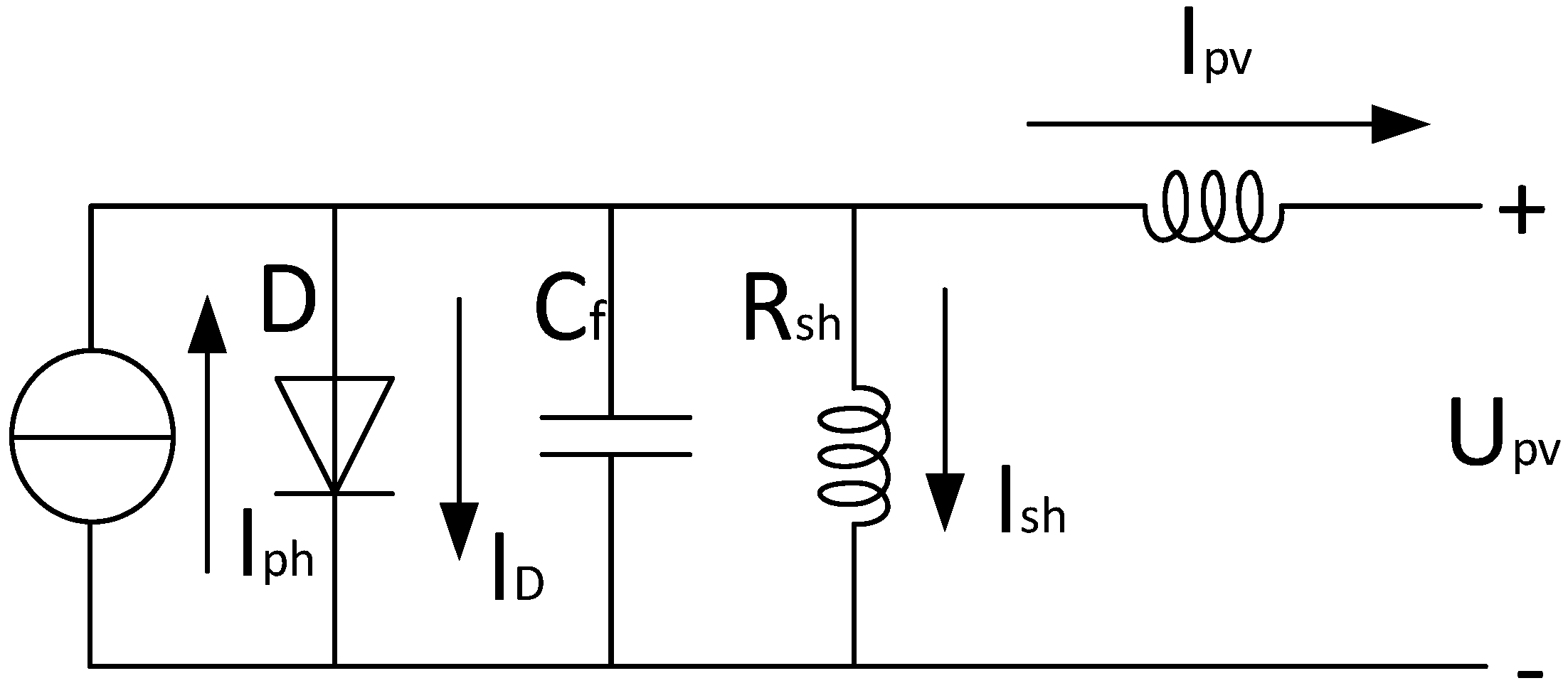
2.3. Photovoltaic Unit Module
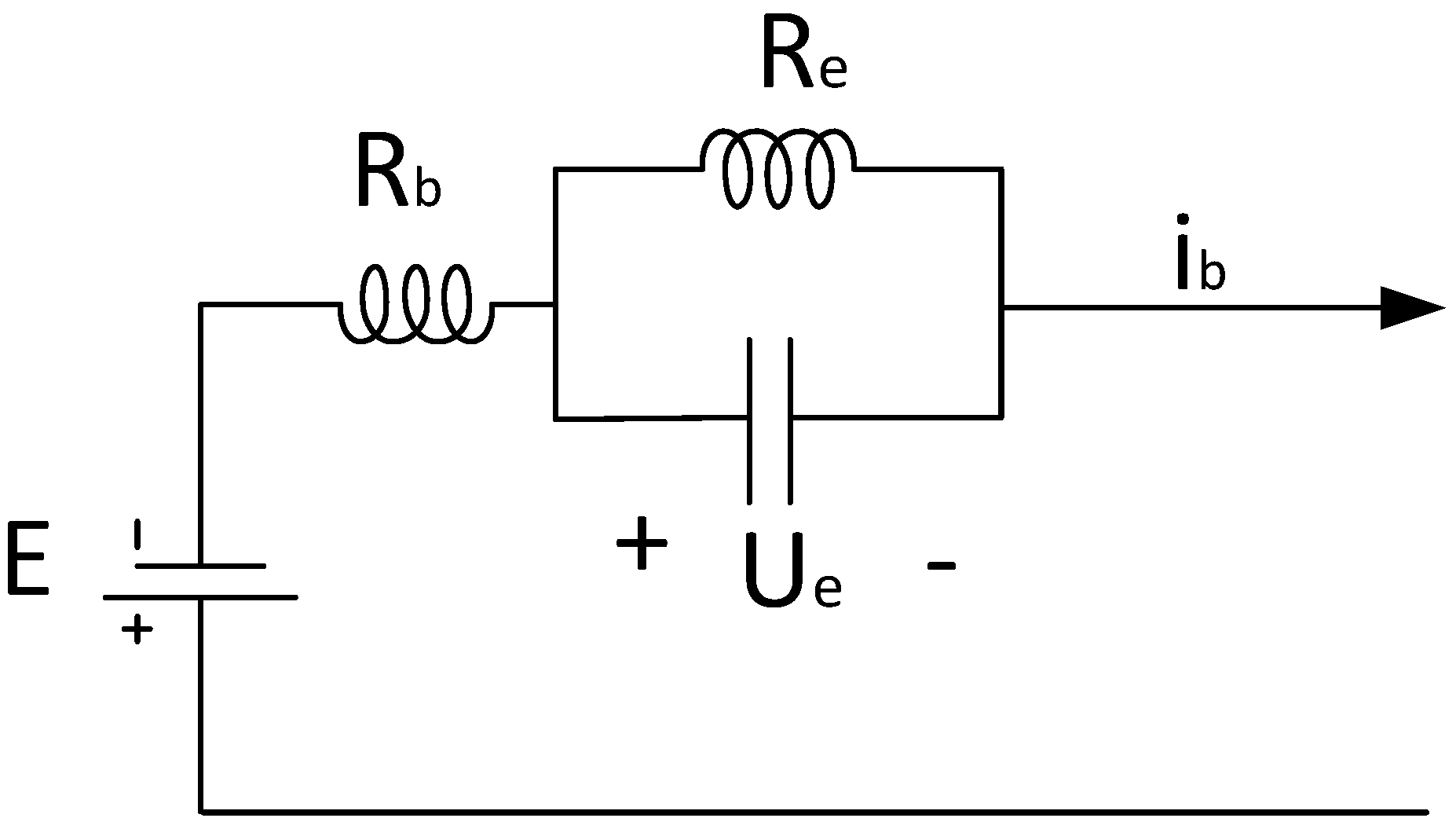
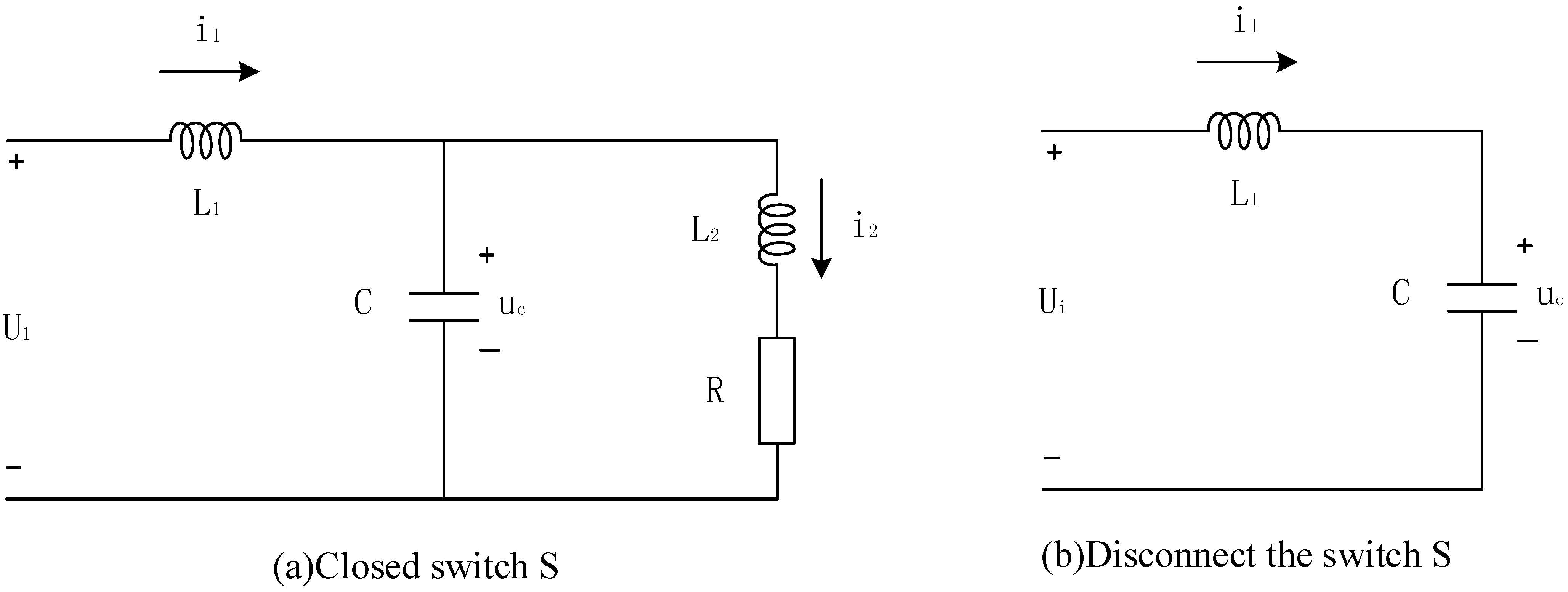
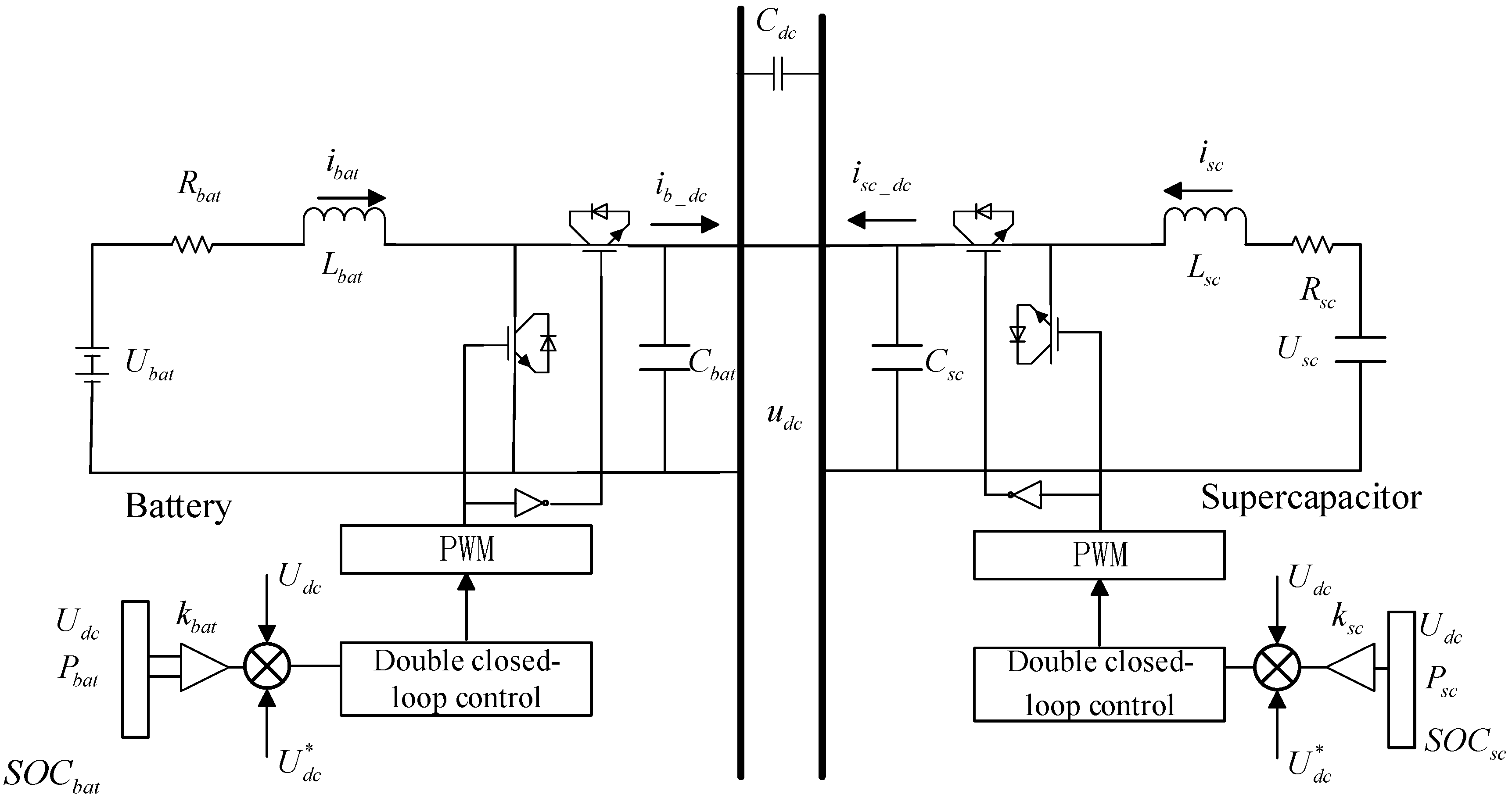
2.4. Hybrid Energy Storage Unit Model
- (1)
- The model of a battery
- (2)
- The model of a super-capacitor
2.5. The Model and Control Strategy of the DC Motor
- The model of the DC motor
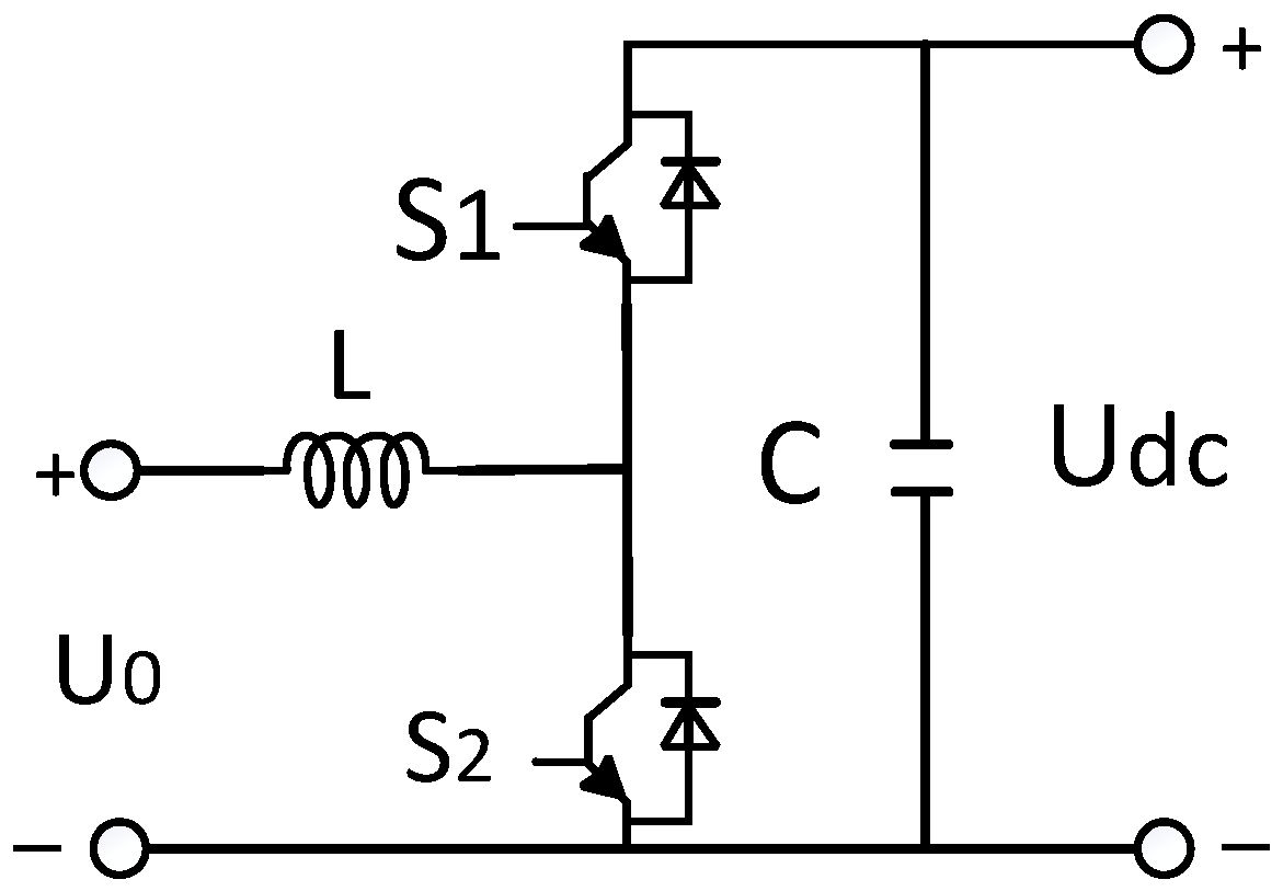
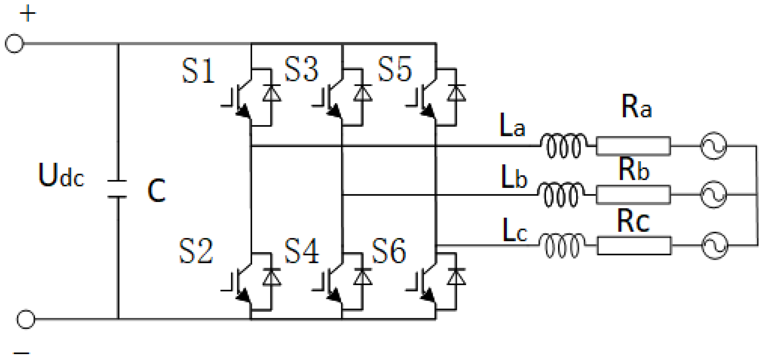
2.6. Modeling Power Converters
- (1)
- Characterization of photovoltaic-side power converter operation
- (2)
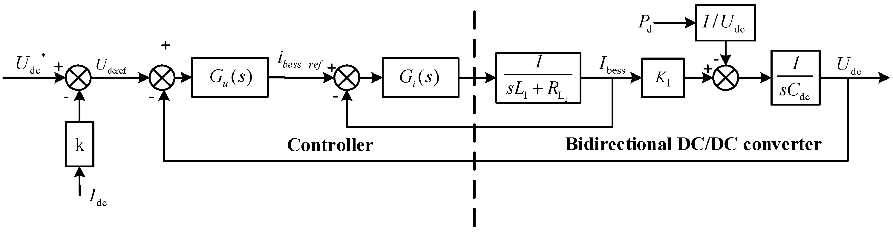
- The operating characteristics of the energy storage power converter
- (3)
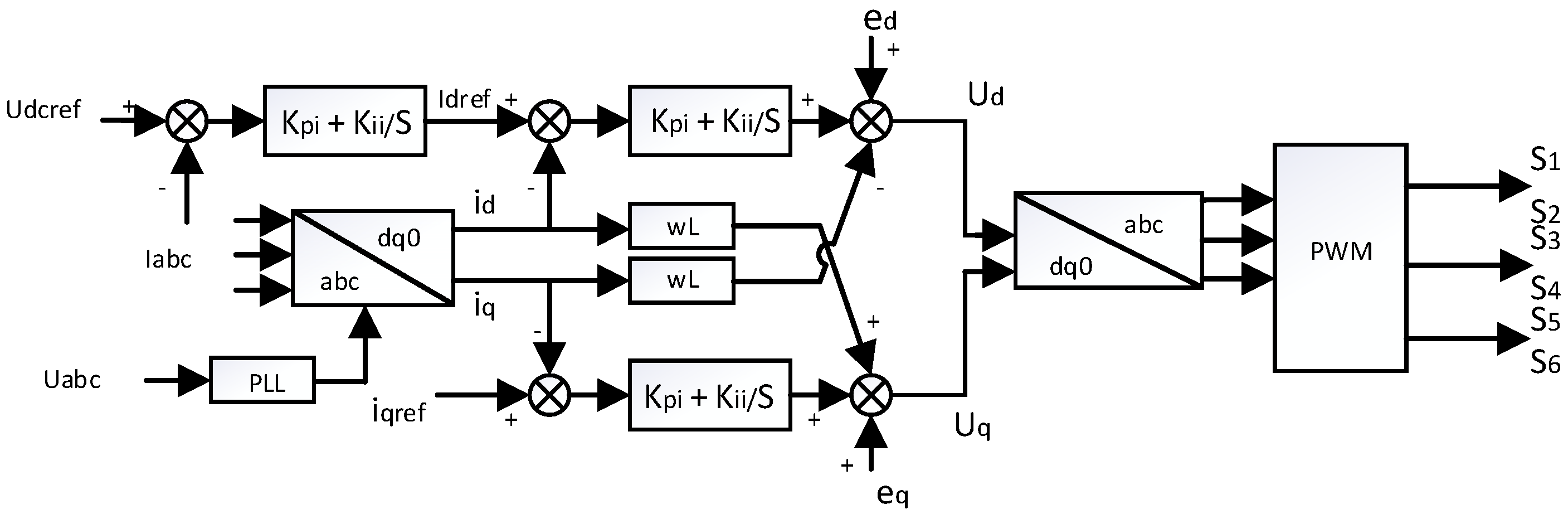
- Grid-connected inverter model and control strategy
3. Fuzzy Droop Control Strategy
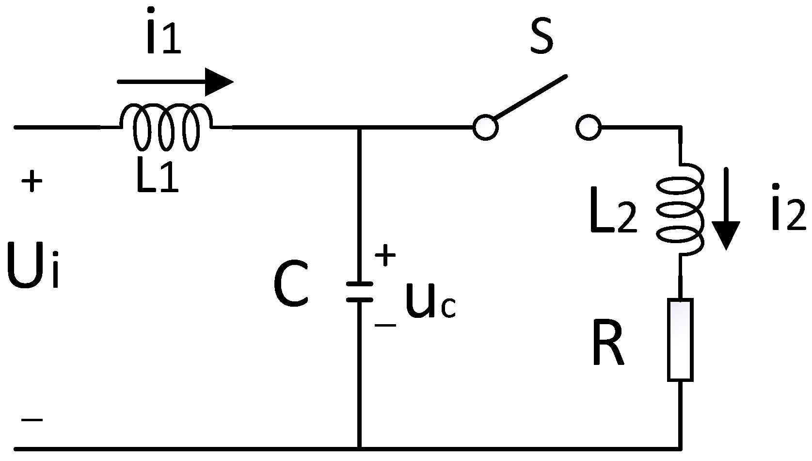
3.1. Classical Droop Control
3.2. Limitations of Traditional Droop Control
3.3. Fuzzy Droop Control of Hybrid Energy Storage System
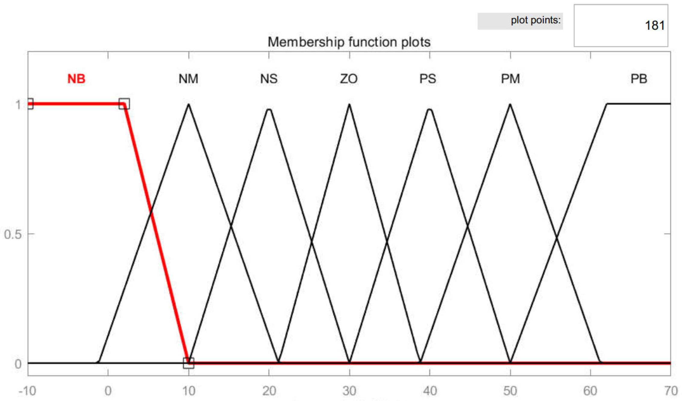
3.3.1. Fuzzy Droop Control in the Battery Branch
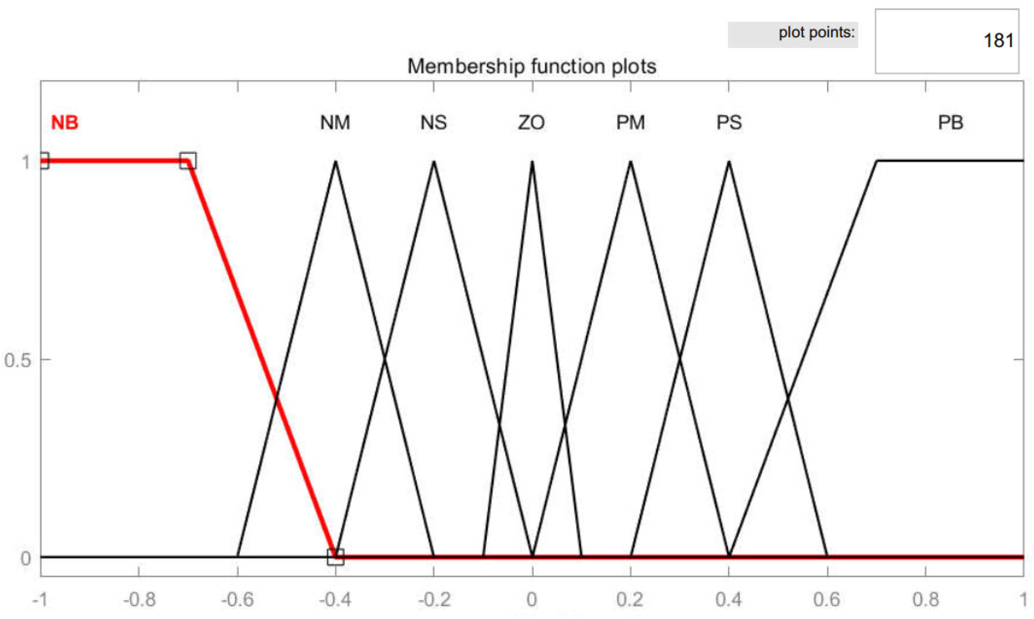
3.3.2. Fuzzy Droop Control of Super-Capacitor Branch
4. Variable Universe Fuzzy Control of HESSs Based on an Improved Harris Hawk Optimization Algorithm
4.1. Harris Hawk Optimization Algorithm
4.1.1. Exploration Phase
4.1.2. Transition Processes of Exploration and Exploitation Phase
4.1.3. Exploitation Phase
- Case 1: Soft Besiege
- Case 2: Hard Besiege
- Case 3: Soft Besiege with Progressive Rapid Dives
- Case 4: Hard Besiege with Progressive Rapid Dives.
4.2. Proposed Algorithm and Its Numerical Experiments
4.2.1. Motivation for Algorithm Design
4.2.2. Fuch Mapping
4.2.3. Golden Sine Strategy
4.2.4. Elitism Lens Imaging Opposition-Based Learning Strategy
4.2.5. The Proposed MHHO Algorithm
- Step 1: Set the algorithm initialization input parameters: the total number of population N, the maximum number of iterations Max_Iteration, convex combination factor of 0.6;
- Step 2: Using Fuch mapping (Equation (31)) to randomly generate the initial population;
- Step 3: According to the fitness function, the initial population is evaluated;
- Step 4: Calculate the fitness value: Calculate the fitness value of each particle individual, record and screen out the best population so far;
- Step 5: Exploration and exploitation phase of the conversion strategy using Equation (21);
- Step 6: Equation (33) is used in the exploration phase of the algorithm;
- Step 7: Equations (22)–(38) are used in the exploitation phase of the algorithm;
- Step 8: If the current number of iterations is less than the maximum number of iterations, the iteration process of step 5 and step 7 is repeated until the set accuracy requirement or the maximum number of iterations is reached, and the optimal individual position and its fitness value are output.
4.2.6. Numerical Experiment
- (1)
- Simulation environment
- (2)
- Benchmark functions and setting
- (3)
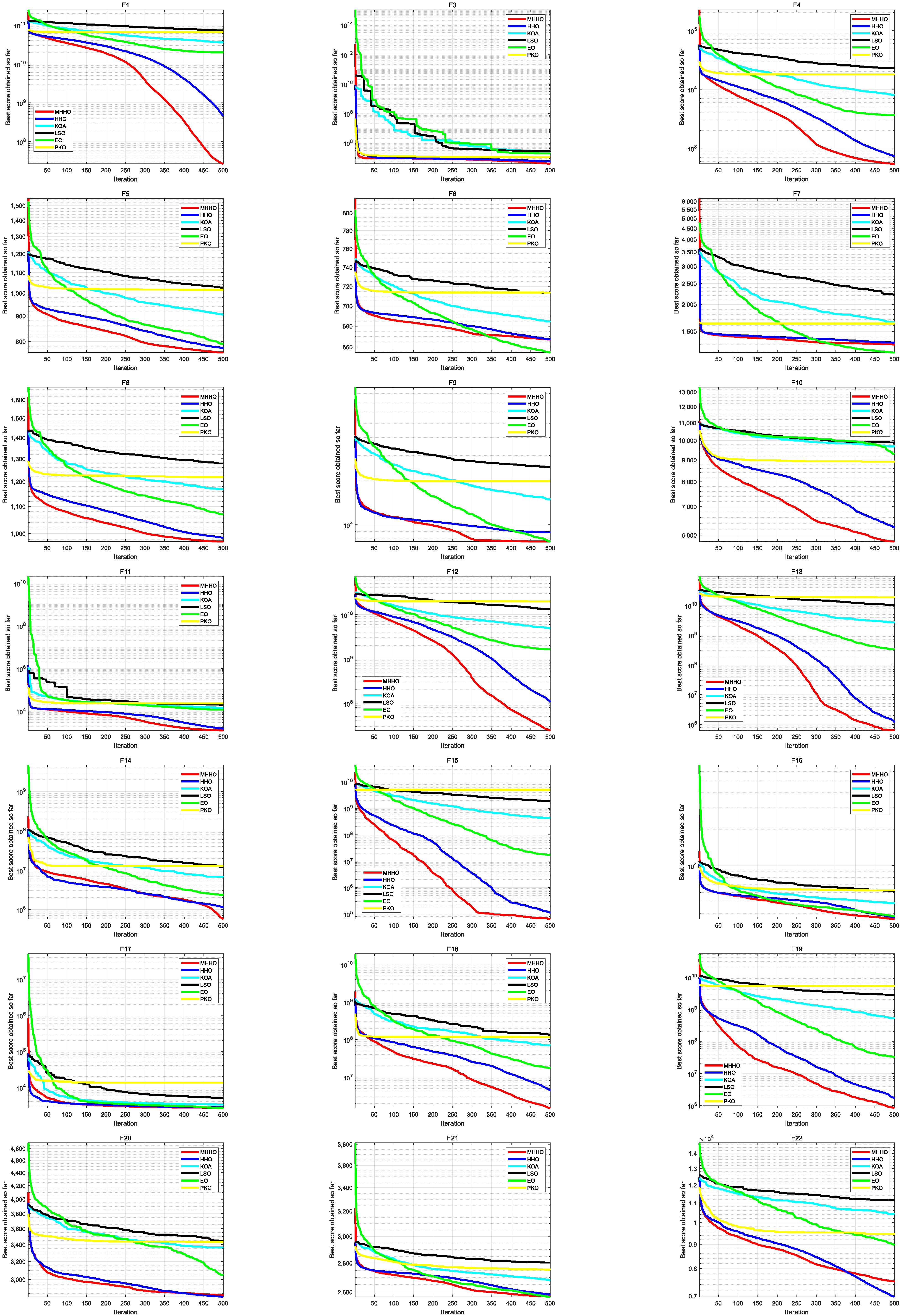
- Comparative analysis of MHHO and other algorithms
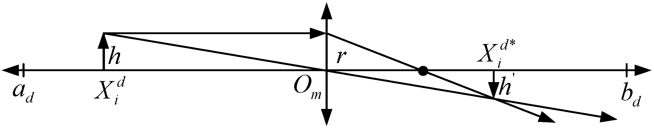
4.3. Variable Universe Fuzzy Control
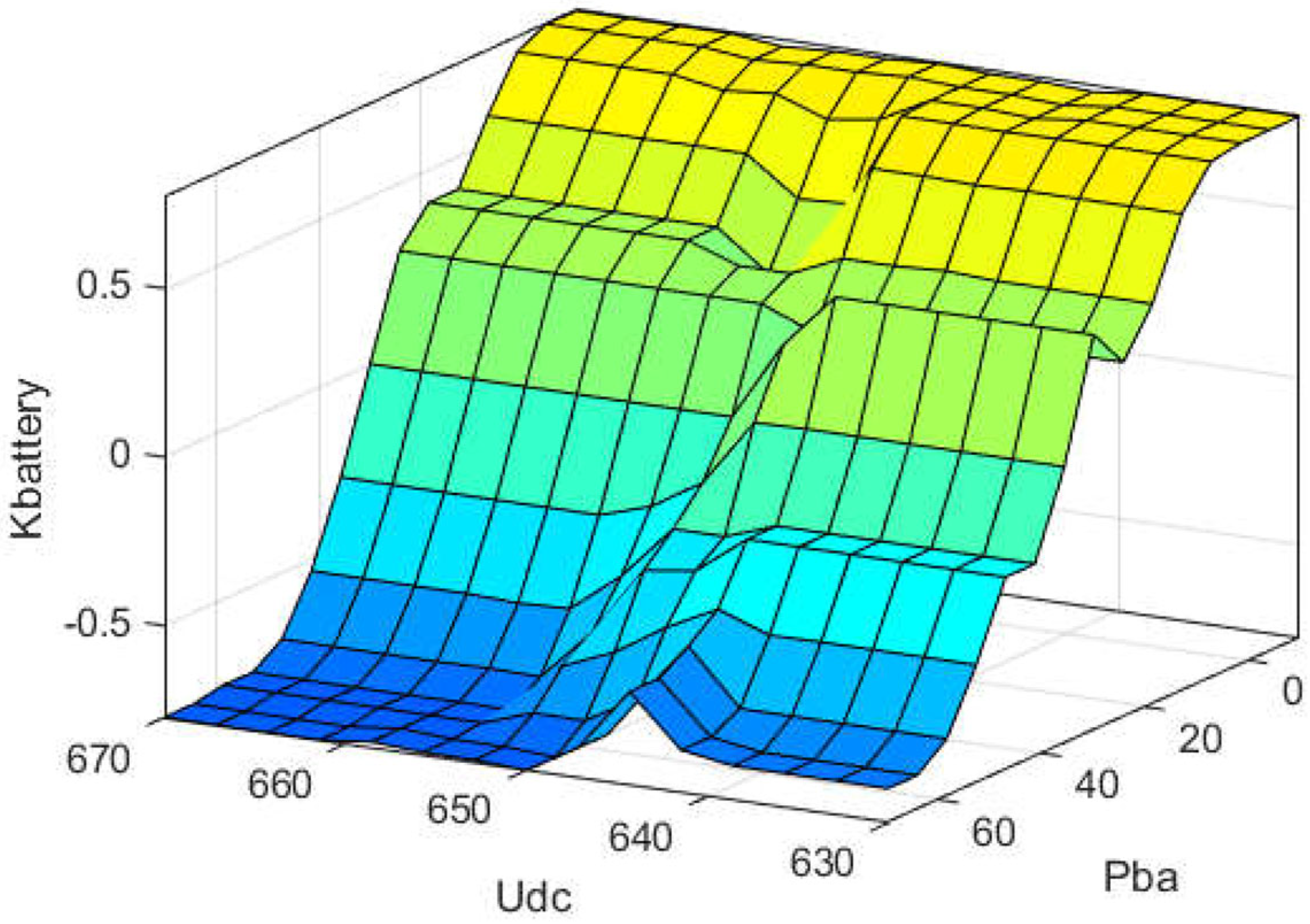
4.4. Variable Universe Fuzzy Droop Control Based on an Improved HHO Algorithm
4.5. Adaptive Variable Universe Fuzzy Droop Control Process Based on MHHO
- Step 1: Parameter initialization for MHHO algorithm;
- Step 2: In the current control cycle, according to the output of the current controlled quantity, the voltage fluctuation of the bus, the of the battery branch and the of the super-capacitor branch are obtained;
- Step 3: Taking the droop Equation (14) as the fitness function, the MHHO algorithm is used to optimize the scaling factor , , , , and ;
- Step 4: Applying the optimal , , , , and which are obtained by the MHHO algorithm to the next control period of the droop control of the PV DC- microgrid with HESSs;
- Step 5: If the control is over, stop; otherwise, go to Step 2.
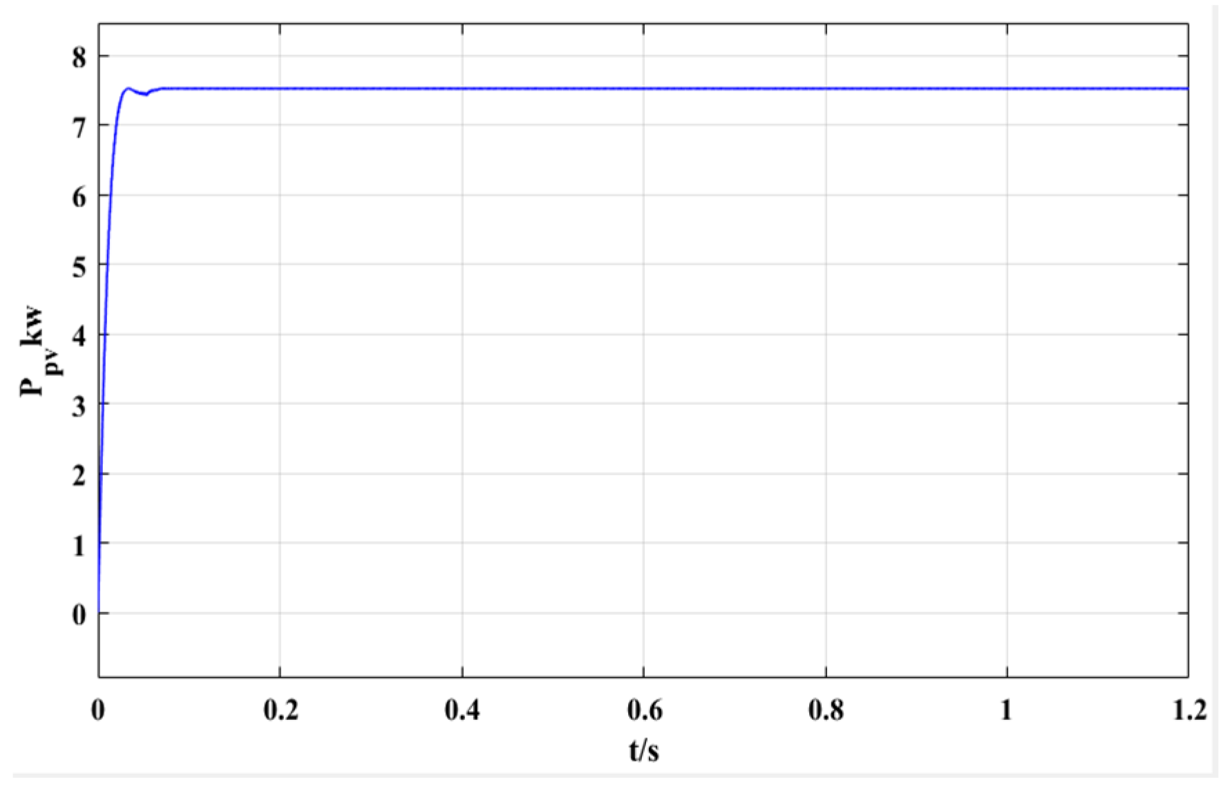
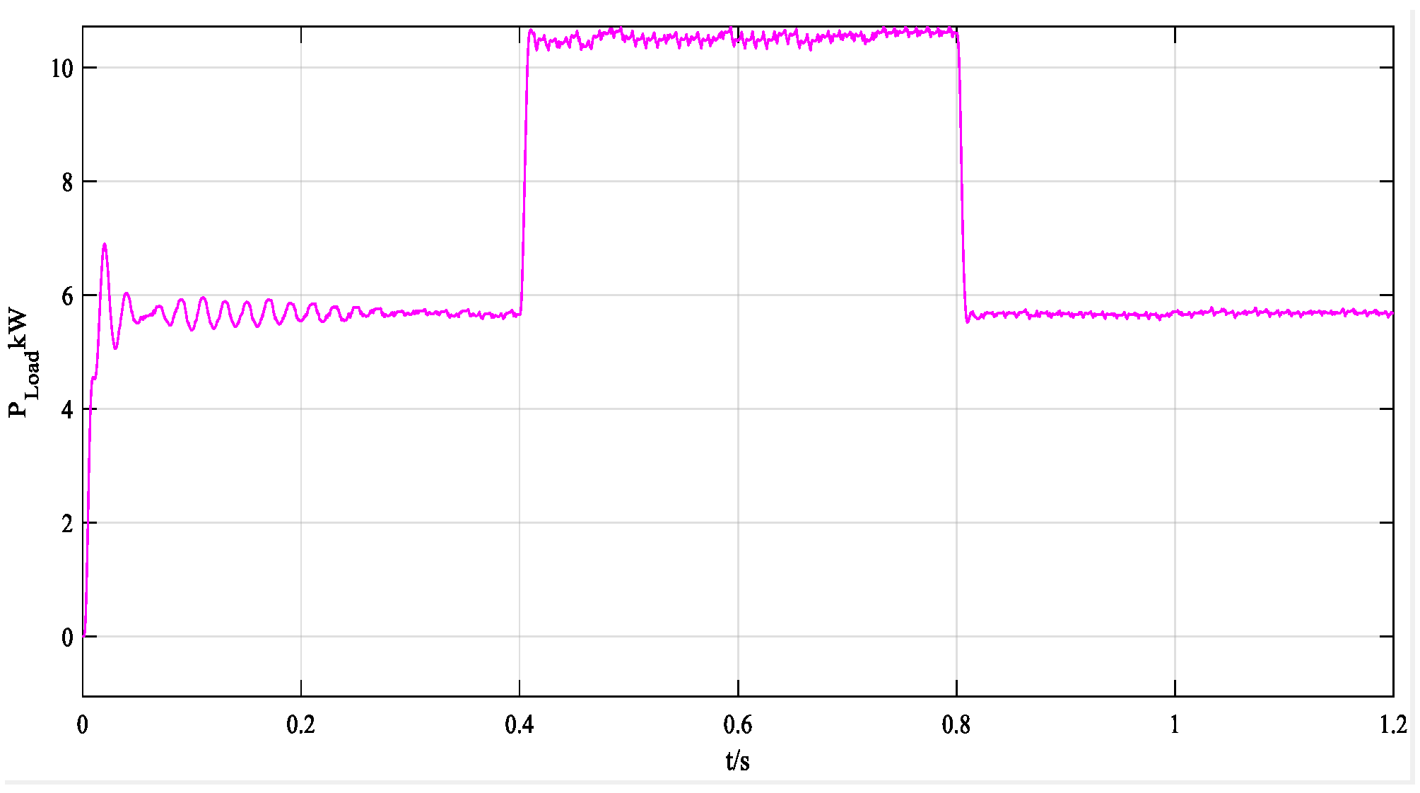
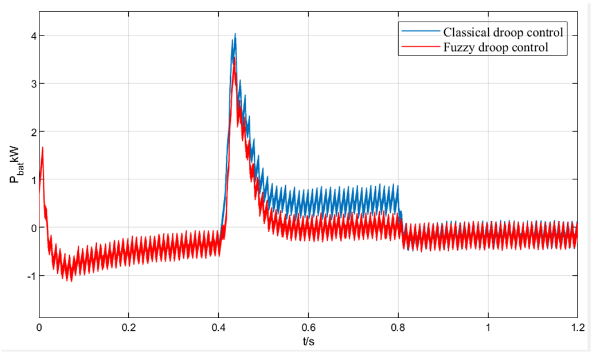
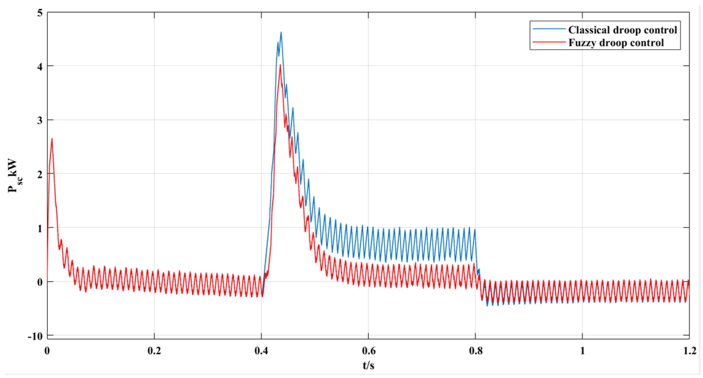
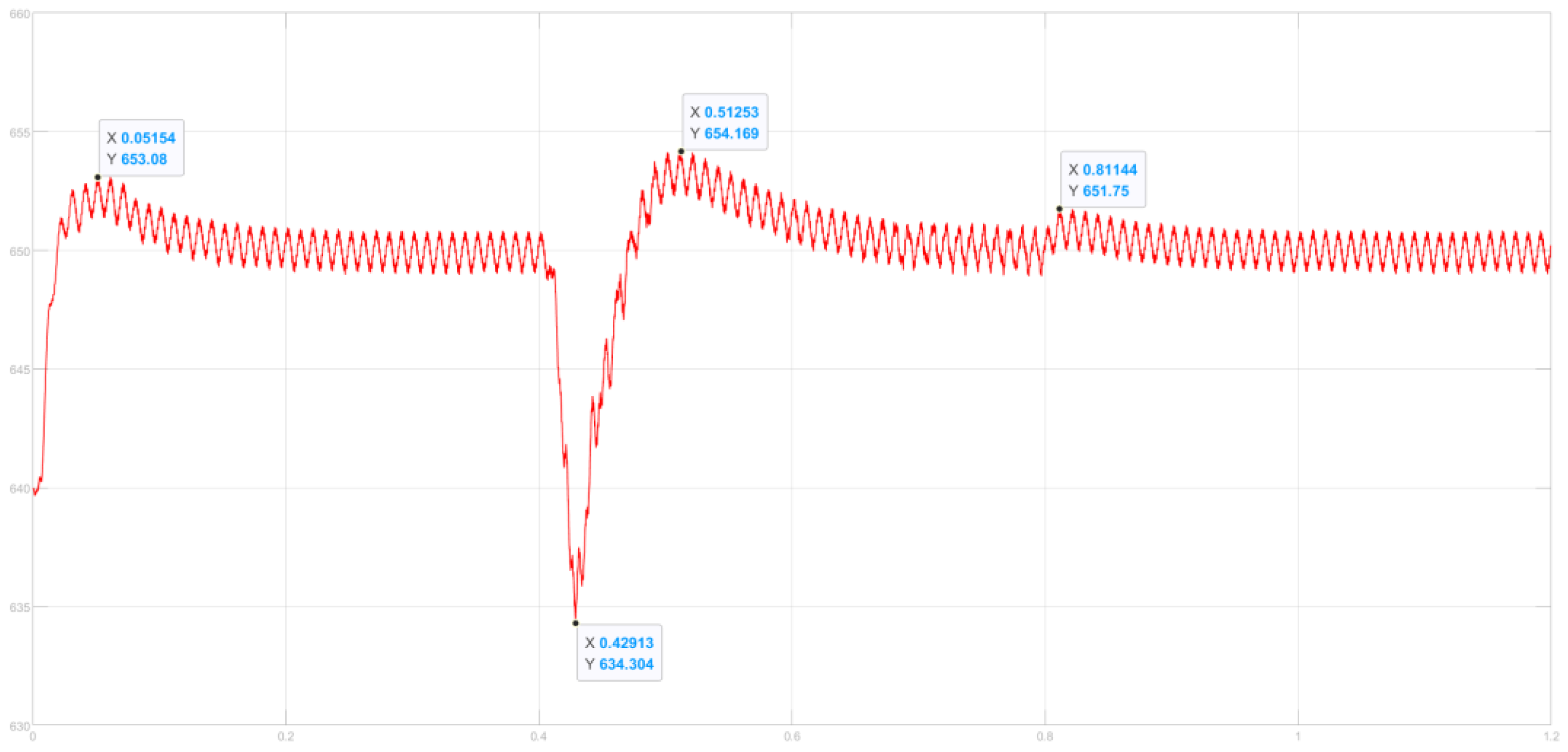
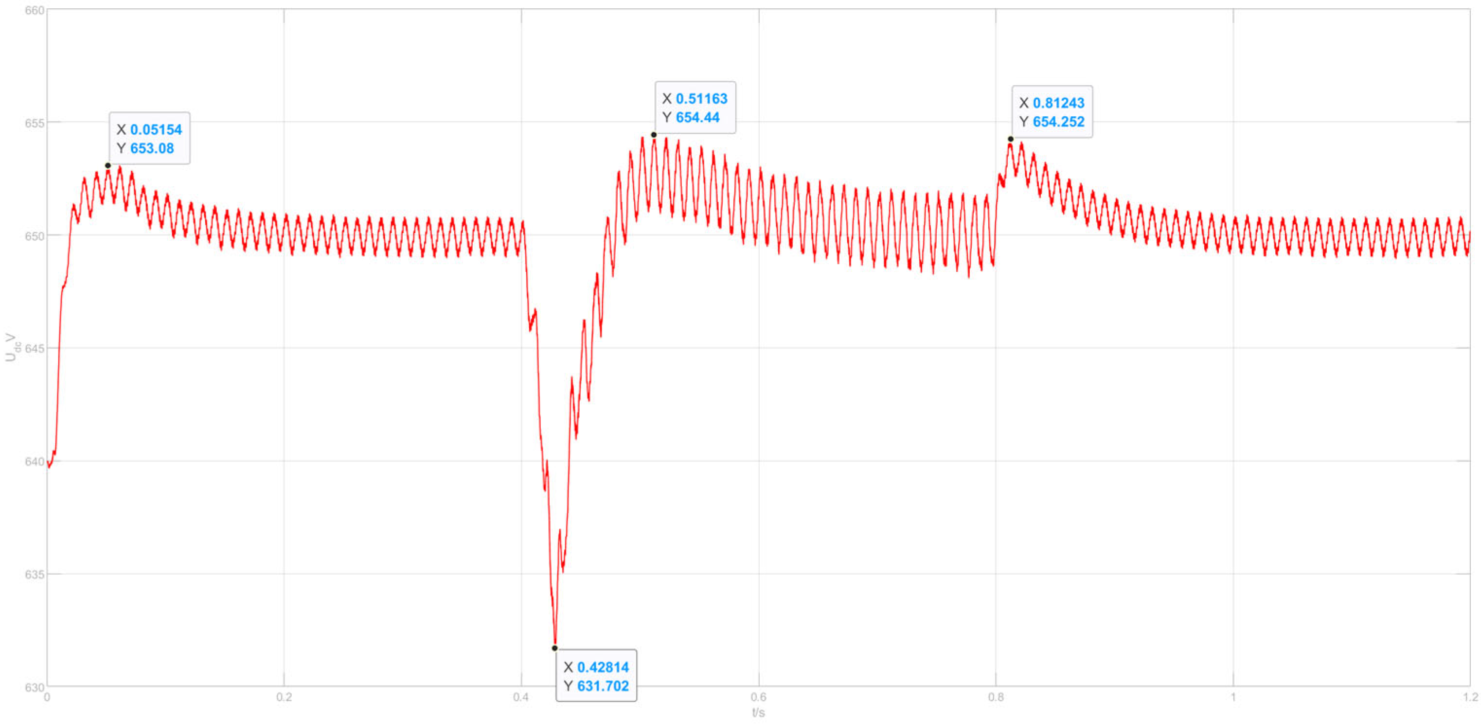
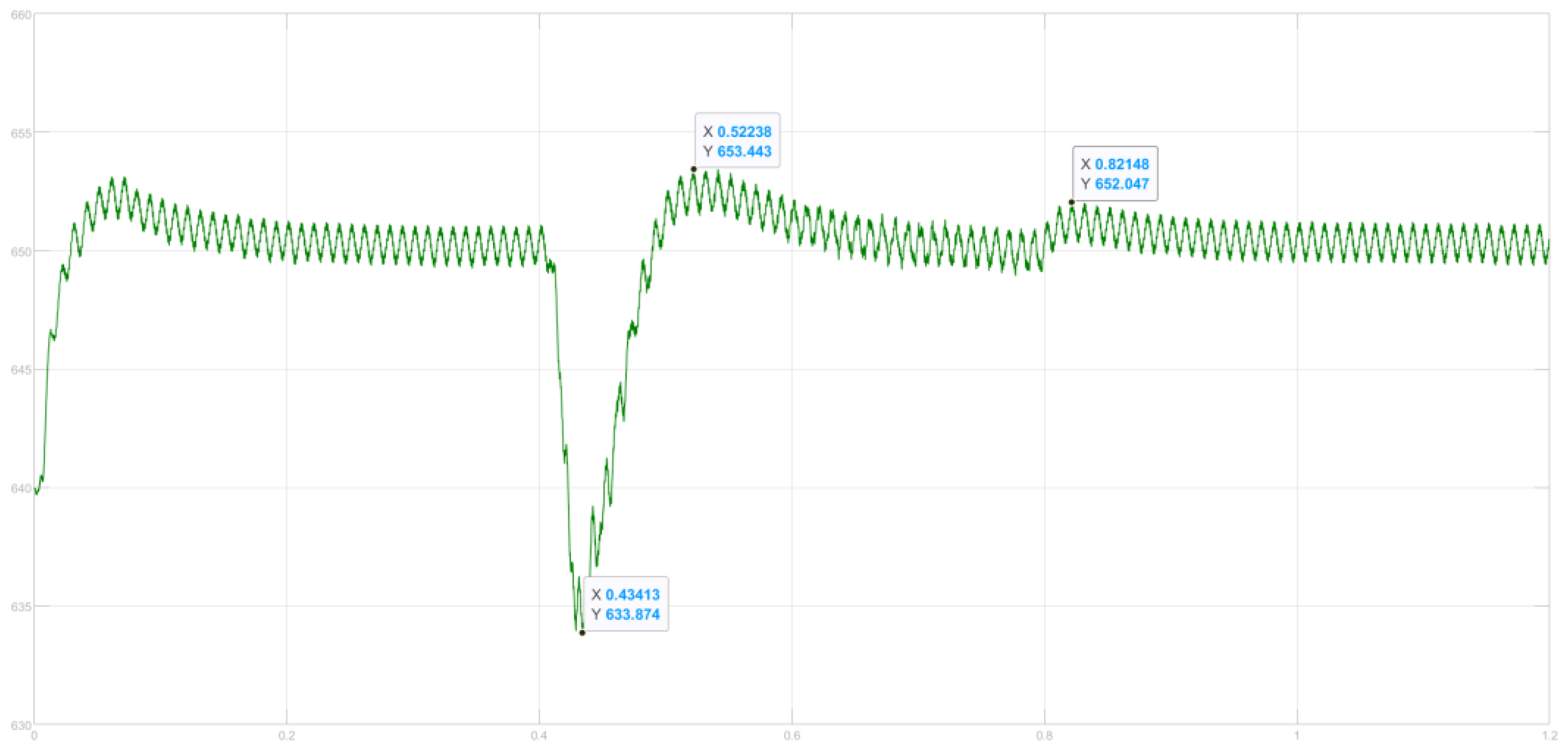
5. Simulation and Results
6. Conclusions
- The introduction of adaptive variable universe fuzzy control enhances the traditional droop control strategy, enabling dynamic adjustment of the initial droop curve coefficient for optimal power distribution.
- The adaptive variable universe fuzzy-droop control based on MHHO outperforms traditional droop control by improving power distribution accuracy, reducing bus voltage fluctuations, and enhancing system robustness.
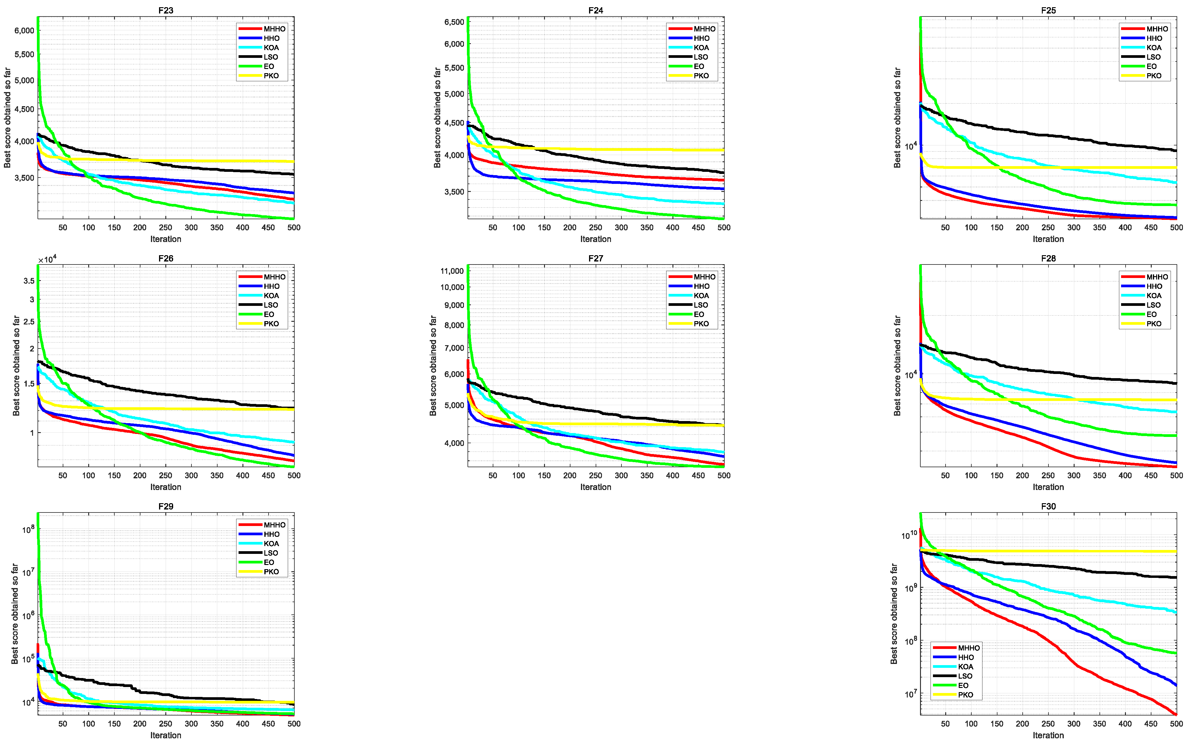
- The MHHO algorithm demonstrates superior performance compared to HHO and other classical and new meta-heuristic algorithms with better performance like KOA, LSO, EO, and PKO.
Author Contributions
Funding
Data Availability Statement
Conflicts of Interest
References
- Papadimitriou, C.N.; Zountouridou, E.I.; Hatziargyriou, N.D. Review of Hierarchical Control in DC Microgrids. Electr. Power Syst. Res. 2015, 122, 159–167. [Google Scholar] [CrossRef]
- Tian, G.; Zheng, Y.; Liu, G.; Zhang, J. SOC Balancing and Coordinated Control Based on Adaptive Droop Coefficient Algorithm for Energy Storage Units in DC Microgrid. Energies 2022, 15, 2943. [Google Scholar] [CrossRef]
- Okwako, O.E.; Lin, Z.-H.; Xin, M.; Premkumar, K.; Rodgers, A.J. Neural Network Controlled Solar PV Battery Powered Unified Power Quality Conditioner for Grid Connected Operation. Energies 2022, 15, 6825. [Google Scholar] [CrossRef]
- Lakhina, U.; Badruddin, N.; Elamvazuthi, I.; Jangra, A.; Huy, T.H.B.; Guerrero, J.M. An Enhanced Multi-Objective Optimizer for Stochastic Generation Optimization in Islanded Renewable Energy Microgrids. Mathematics 2023, 11, 2079. [Google Scholar] [CrossRef]
- Chen, M.; Ma, S.; Wan, H.; Wu, J.; Jiang, Y. Distributed Control Strategy for DC Microgrids of Photovoltaic Energy Storage Systems in Off-Grid Operation. Energies 2018, 11, 2637. [Google Scholar] [CrossRef]
- Tobajas, J.; Garcia-Torres, F.; Roncero-Sánchez, P.; Vázquez, J.; Bellatreche, L.; Nieto, E. Resilience-Oriented Schedule of Microgrids with Hybrid Energy Storage System Using Model Predictive Control. Appl. Energy 2022, 306, 118092. [Google Scholar] [CrossRef]
- Lu, M.-Z.; Guo, Z.-W.; Liaw, C.-M. A Battery/Supercapacitor Hybrid Powered EV SRM Drive and Microgrid Incorporated Operations. IEEE Trans. Transp. Electrif. 2021, 7, 2848–2863. [Google Scholar] [CrossRef]
- Yin, C.; Wu, H.; Locment, F.; Sechilariu, M. Energy Management of DC Microgrid Based on Photovoltaic Combined with Diesel Generator and Supercapacitor. Energy Convers. Manag. 2017, 132, 14–27. [Google Scholar] [CrossRef]
- Dragicevic, T.; Guerrero, J.M.; Vasquez, J.C.; Skrlec, D. Supervisory Control of an Adaptive-Droop Regulated DC Microgrid with Battery Management Capability. IEEE Trans. Power Electron. 2014, 29, 695–706. [Google Scholar] [CrossRef]
- Zhou, H.; Bhattacharya, T.; Tran, D.; Siew, T.S.T.; Khambadkone, A.M. Composite Energy Storage System Involving Battery and Ultracapacitor with Dynamic Energy Management in Microgrid Applications. IEEE Trans. Power Electron. 2011, 26, 923–930. [Google Scholar] [CrossRef]
- Wang, S.; Tang, Y.; Shi, J.; Gong, K.; Liu, Y.; Ren, L.; Li, J. Design and Advanced Control Strategies of a Hybrid Energy Storage System for the Grid Integration of Wind Power Generations. IET Renew. Power Gener. 2015, 9, 89–98. [Google Scholar] [CrossRef]
- Xiao, G.; Xu, F.; Tong, L.; Xu, H.; Zhu, P. A Hybrid Energy Storage System Based on Self-Adaptive Variational Mode Decomposition to Smooth Photovoltaic Power Fluctuation. J. Energy Storage 2022, 55, 105509. [Google Scholar] [CrossRef]
- Anand, S.; Fernandes, B.G.; Guerrero, J. Distributed Control to Ensure Proportional Load Sharing and Improve Voltage Regulation in Low-Voltage DC Microgrids. IEEE Trans. Power Electron. 2013, 28, 1900–1913. [Google Scholar] [CrossRef]
- Xiao, J.; Setyawan, L. Hierarchical Control of Hybrid Energy Storage System in DC Microgrids. IEEE Trans. Ind. Electron. 2015, 62, 4915–4924. [Google Scholar] [CrossRef]
- Ding, M.; Lin, D.; Chen, Z.; Luo, Y.; Zhao, B. A Control Strategy for Hybrid Energy Storage Systems. Proc. CSEE 2012, 32, 1–6+184. [Google Scholar] [CrossRef]
- Malik, S.M.; Sun, Y.; Hu, J. An Adaptive Virtual Capacitive Droop for Hybrid Energy Storage System in DC Microgrid. J. Energy Storage 2023, 70, 107809. [Google Scholar] [CrossRef]
- Li, J.; Yang, Q.; Robinson, F.; Liang, F.; Zhang, M.; Yuan, W. Design and Test of a New Droop Control Algorithm for a SMES/Battery Hybrid Energy Storage System. Energy 2017, 118, 1110–1122. [Google Scholar] [CrossRef]
- Vafamand, A.; Vafamand, N.; Zarei, J.; Razavi-Far, R.; Dragicevic, T. Intelligent Multiobjective NSBGA-II Control of Power Converters in DC Microgrids. IEEE Trans. Ind. Electron. 2021, 68, 10806–10814. [Google Scholar] [CrossRef]
- Holland, J.H. Genetic Algorithms and the Optimal Allocation of Trials. SIAM J. Comput. 1973, 2, 88–105. [Google Scholar] [CrossRef]
- Ahmad, M.F.; Isa, N.A.M.; Lim, W.H.; Ang, K.M. Differential Evolution: A Recent Review Based on State-of-the-Art Works. Alex. Eng. J. 2022, 61, 3831–3872. [Google Scholar] [CrossRef]
- Kennedy, J.; Eberhart, R. Particle Swarm Optimization. In Proceedings of the ICNN’95—International Conference on Neural Networks, Perth, WA, Australia, 27 November–1 December 1995; IEEE: Piscataway, NJ, USA, 1995; Volume 4, pp. 1942–1948. [Google Scholar]
- Bouaouda, A.; Hashim, F.A.; Sayouti, Y.; Hussien, A.G. Pied Kingfisher Optimizer: A New Bio-Inspired Algorithm for Solving Numerical Optimization and Industrial Engineering Problems. Neural Comput. Appl. 2024, 16, 1–59. [Google Scholar] [CrossRef]
- Abdollahzadeh, B.; Gharehchopogh, F.S.; Khodadadi, N.; Mirjalili, S. Mountain Gazelle Optimizer: A New Nature-Inspired Metaheuristic Algorithm for Global Optimization Problems. Adv. Eng. Softw. 2022, 174, 103282. [Google Scholar] [CrossRef]
- Harifi, S.; Mohammadzadeh, J.; Khalilian, M.; Ebrahimnejad, S. Giza Pyramids Construction: An Ancient-Inspired Metaheuristic Algorithm for Optimization. Evol. Intell. 2021, 14, 1743–1761. [Google Scholar] [CrossRef]
- Ekinci, S.; Izci, D.; Yilmaz, M. Simulated Annealing Aided Artificial Hummingbird Optimizer for Infinite Impulse Response System Identification. IEEE Access 2023, 11, 88627–88636. [Google Scholar] [CrossRef]
- Abdel-Basset, M.; Mohamed, R.; Azeem, S.A.A.; Jameel, M.; Abouhawwash, M. Kepler Optimization Algorithm: A New Metaheuristic Algorithm Inspired by Kepler’s Laws of Planetary Motion. Knowl.-Based Syst. 2023, 268, 110454. [Google Scholar] [CrossRef]
- Abdel-Basset, M.; Mohamed, R.; Sallam, K.M.; Chakrabortty, R.K. Light Spectrum Optimizer: A Novel Physics-Inspired Metaheuristic Optimization Algorithm. Mathematics 2022, 10, 3466. [Google Scholar] [CrossRef]
- Faramarzi, A.; Heidarinejad, M.; Stephens, B.; Mirjalili, S. Equilibrium Optimizer: A Novel Optimization Algorithm. Knowl.-Based Syst. 2020, 191, 105190. [Google Scholar] [CrossRef]
- Tanyildizi, E.; Demir, G. Golden Sine Algorithm: A Novel Math-Inspired Algorithm. Adv. Electr. Comp. Eng. 2017, 17, 71–78. [Google Scholar] [CrossRef]
- Lam, A.Y.S.; Li, V.O.K. Chemical Reaction Optimization: A Tutorial: (Invited Paper). Memetic Comput. 2012, 4, 3–17. [Google Scholar] [CrossRef]
- Talatahari, S.; Azizi, M.; Tolouei, M.; Talatahari, B.; Sareh, P. Crystal Structure Algorithm (CryStAl): A Metaheuristic Optimization Method. IEEE Access 2021, 9, 71244–71261. [Google Scholar] [CrossRef]
- Trojovska, E.; Dehghani, M.; Trojovsky, P. Fennec Fox Optimization: A New Nature-Inspired Optimization Algorithm. IEEE Access 2022, 10, 84417–84443. [Google Scholar] [CrossRef]
- Ray, T.; Liew, K.M. Society and Civilization: An Optimization Algorithm Based on the Simulation of Social Behavior. IEEE Trans. Evol. Computat. 2003, 7, 386–396. [Google Scholar] [CrossRef]
- Sang, H.-Y.; Duan, P.-Y.; Li, J.-Q. An Effective Invasive Weed Optimization Algorithm for Scheduling Semiconductor Final Testing Problem. Swarm Evol. Comput. 2018, 38, 42–53. [Google Scholar] [CrossRef]
- Liu, Y.; Liu, J.; Ma, L.; Tian, L. Artificial Root Foraging Optimizer Algorithm with Hybrid Strategies. Saudi J. Biol. Sci. 2017, 24, 268–275. [Google Scholar] [CrossRef]
- Geem, Z.W.; Kim, J.H.; Loganathan, G.V. A New Heuristic Optimization Algorithm: Harmony Search. Simulation 2001, 76, 60–68. [Google Scholar] [CrossRef]
- Mora-Gutiérrez, R.A.; Ramírez-Rodríguez, J.; Rincón-García, E.A. An Optimization Algorithm Inspired by Musical Composition. Artif. Intell. Rev. 2014, 41, 301–315. [Google Scholar] [CrossRef]
- Moghdani, R.; Salimifard, K. Volleyball Premier League Algorithm. Appl. Soft Comput. 2018, 64, 161–185. [Google Scholar] [CrossRef]
- Ma, B.; Hu, Y.; Lu, P.; Liu, Y. Running City Game Optimizer: A Game-Based Metaheuristic Optimization Algorithm for Global Optimization. J. Comput. Des. Eng. 2023, 10, 65–107. [Google Scholar] [CrossRef]
- Abualigah, L.; Diabat, A.; Mirjalili, S.; Abd Elaziz, M.; Gandomi, A.H. The Arithmetic Optimization Algorithm. Comput. Methods Appl. Mech. Eng. 2021, 376, 113609. [Google Scholar] [CrossRef]
- Mirjalili, S. SCA: A Sine Cosine Algorithm for Solving Optimization Problems. Knowl.-Based Syst. 2016, 96, 120–133. [Google Scholar] [CrossRef]
- Pisinger, D.; Ropke, S. Large Neighborhood Search. In Handbook of Metaheuristics; Gendreau, M., Potvin, J.-Y., Eds.; International Series in Operations Research & Management Science; Springer: Boston, MA, USA, 2010; Volume 146, pp. 399–419. ISBN 978-1-4419-1663-1. [Google Scholar]
- Yu, C.; Lahrichi, N.; Matta, A. Optimal Budget Allocation Policy for Tabu Search in Stochastic Simulation Optimization. Comput. Oper. Res. 2023, 150, 106046. [Google Scholar] [CrossRef]
- Heidari, A.A.; Mirjalili, S.; Faris, H.; Aljarah, I.; Mafarja, M.; Chen, H. Harris Hawks Optimization: Algorithm and Applications. Future Gener. Comput. Syst. 2019, 97, 849–872. [Google Scholar] [CrossRef]
- Luo, J.; Gao, S.; Wei, X.; Tian, Z. Adaptive Energy Management Strategy for High-Speed Railway Hybrid Energy Storage System Based on Double-Layer Fuzzy Logic Control. Int. J. Electr. Power Energy Syst. 2024, 156, 109739. [Google Scholar] [CrossRef]
- Augustine, S.; Mishra, M.K.; Lakshminarasamma, N. A Unified Control Scheme for a Standalone Solar-PV Low Voltage DC Microgrid System With HESS. IEEE J. Emerg. Sel. Top. Power Electron. 2020, 8, 1351–1360. [Google Scholar] [CrossRef]
- Celikel, R.; Yilmaz, M.; Gundogdu, A. A Voltage Scanning-Based MPPT Method for PV Power Systems under Complex Partial Shading Conditions. Renew. Energy 2022, 184, 361–373. [Google Scholar] [CrossRef]
- Zhang, M.; Xu, Q.; Zhang, C.; Nordstrom, L.; Blaabjerg, F. Decentralized Coordination and Stabilization of Hybrid Energy Storage Systems in DC Microgrids. IEEE Trans. Smart Grid 2022, 13, 1751–1761. [Google Scholar] [CrossRef]
- Ekinci, S.; Izci, D.; Yilmaz, M. Efficient Speed Control for DC Motors Using Novel Gazelle Simplex Optimizer. IEEE Access 2023, 11, 105830–105842. [Google Scholar] [CrossRef]
- Cai, H.; Xiang, J.; Wei, W.; Chen, M.Z.Q. Droop Control for PV Sources in DC Microgrids. IEEE Trans. Power Electron. 2018, 33, 7708–7720. [Google Scholar] [CrossRef]
- Xu, Q.; Hu, X.; Wang, P.; Xiao, J.; Tu, P.; Wen, C.; Lee, M.Y. A Decentralized Dynamic Power Sharing Strategy for Hybrid Energy Storage System in Autonomous DC Microgrid. IEEE Trans. Ind. Electron. 2017, 64, 5930–5941. [Google Scholar] [CrossRef]
- Diaz, N.L.; Dragicevic, T.; Vasquez, J.C.; Guerrero, J.M. Intelligent Distributed Generation and Storage Units for DC Microgrids—A New Concept on Cooperative Control Without Communications Beyond Droop Control. IEEE Trans. Smart Grid 2014, 5, 2476–2485. [Google Scholar] [CrossRef]
- Koupaei, J.A.; Hosseini, S.M.M.; Ghaini, F.M.M. A New Optimization Algorithm Based on Chaotic Maps and Golden Section Search Method. Eng. Appl. Artif. Intell. 2016, 50, 201–214. [Google Scholar] [CrossRef]
- Li, L.; Liu, K.; Wang, L.; Sun, L.; Zhang, Z.; Guo, H. Fault Diagnosis of Balancing Machine Based on ISSA-ELM. Comput. Intell. Neurosci. 2022, 2022, 4981022. [Google Scholar] [CrossRef] [PubMed]
- Tizhoosh, H.R. Opposition-Based Learning: A New Scheme for Machine Intelligence. In Proceedings of the International Conference on Computational Intelligence for Modelling, Control and Automation and International Conference on Intelligent Agents, Web Technologies and Internet Commerce (CIMCA-IAWTIC’06), Vienna, Austria, 28–30 November 2005; IEEE: Piscataway, NJ, USA, 2005; Volume 1, pp. 695–701. [Google Scholar]
- Feng, W.; Zhang, W.; Huang, S. A Novel Parameter Estimation Method for PMSM by Using Chaotic Particle Swarm Optimization With Dynamic Self-Optimization. IEEE Trans. Veh. Technol. 2023, 72, 8424–8432. [Google Scholar] [CrossRef]
- Abdel-Basset, M.; Mohamed, R.; Jameel, M.; Abouhawwash, M. Nutcracker Optimizer: A Novel Nature-Inspired Metaheuristic Algorithm for Global Optimization and Engineering Design Problems. Knowl.-Based Syst. 2023, 262, 110248. [Google Scholar] [CrossRef]
- Shareef, H.; Ibrahim, A.A.; Mutlag, A.H. Lightning Search Algorithm. Appl. Soft Comput. 2015, 36, 315–333. [Google Scholar] [CrossRef]
- Pang, H.; Liu, F.; Xu, Z. Variable Universe Fuzzy Control for Vehicle Semi-Active Suspension System with MR Damper Combining Fuzzy Neural Network and Particle Swarm Optimization. Neurocomputing 2018, 306, 130–140. [Google Scholar] [CrossRef]


| NB | NM | NS | ZO | PS | PM | PB | |
|---|---|---|---|---|---|---|---|
| PB | PB | PM | PS | NS | NS | NM | |
| PB | PB | PM | PS | NS | NS | NM | |
| PB | PM | PS | ZO | NS | NM | NB | |
| CE | PB | PM | PS | ZO | NS | NM | NB |
| PB | PM | PS | ZO | NS | NM | NB | |
| PB | PS | PS | ZO | NM | NB | NB | |
| PB | PS | PS | ZO | NM | NB | NB |
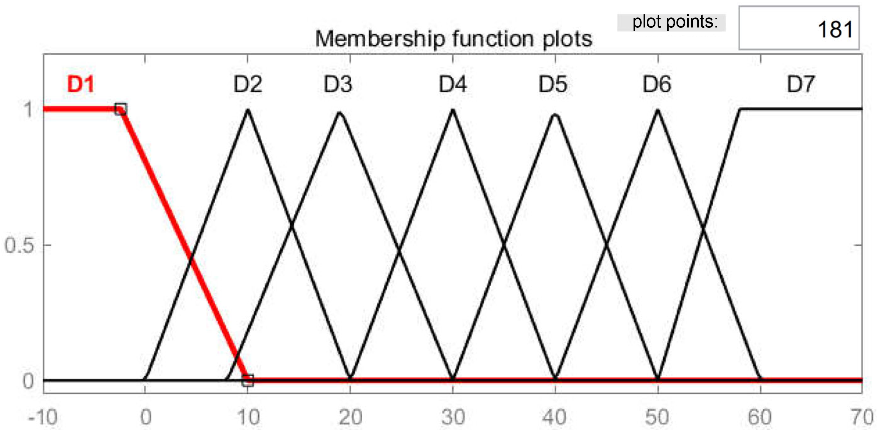
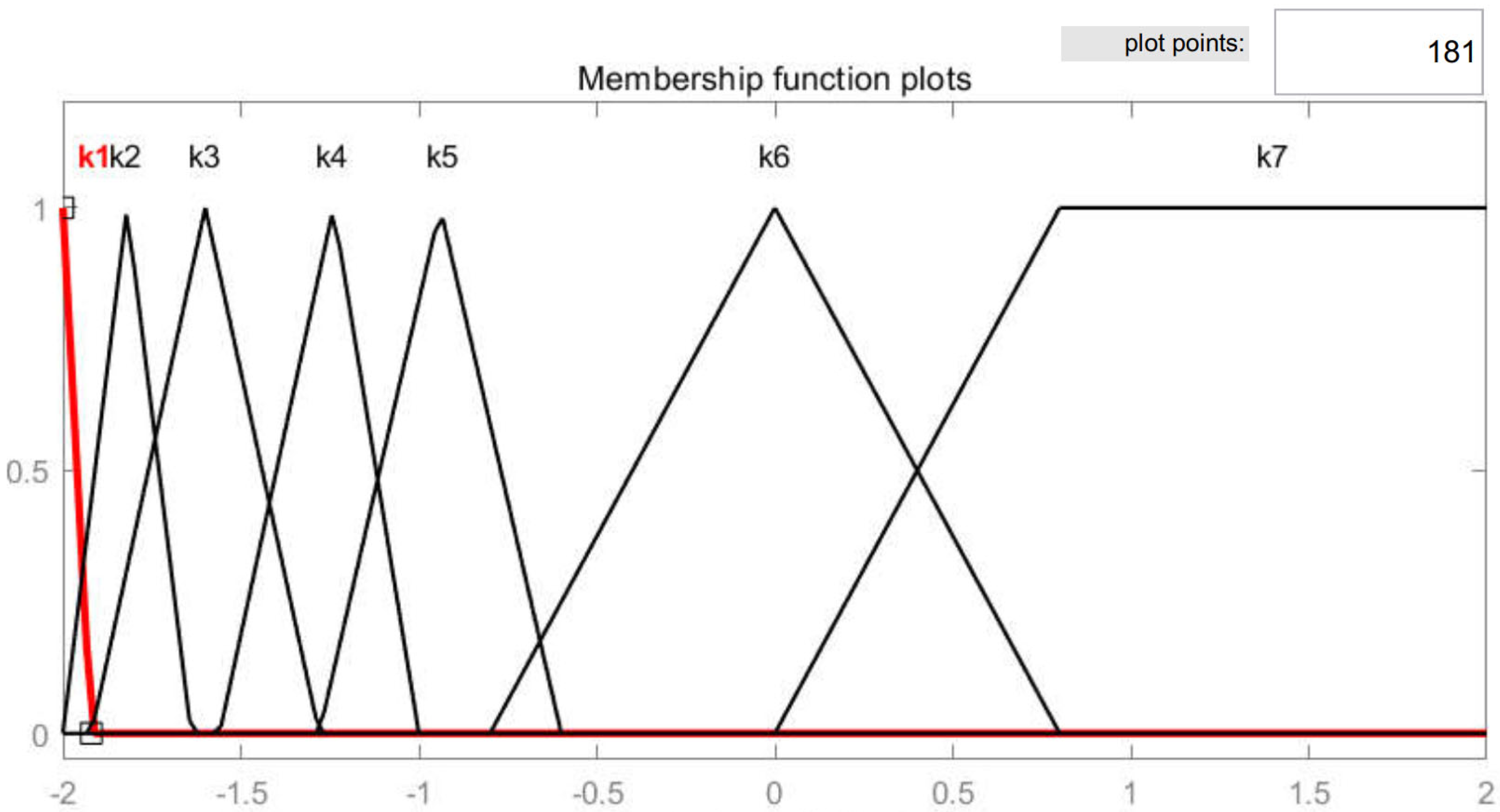
| D1 | D2 | D3 | D4 | D5 | D6 | D7 | |
|---|---|---|---|---|---|---|---|
| Benchmarks | MHHO | HHO | KOA | LSO | ×10O | PKO | |
|---|---|---|---|---|---|---|---|
| F1 | Mean | 2.68 × 10⁷ | 4.41 × 10⁸ | 3.58 × 10¹⁰ | 7.16 × 10¹⁰ | 1.99 × 10¹⁰ | 6.67 × 10¹⁰ |
| Std | 7.86 × 10⁶ | 2.47 × 10⁸ | 7.74 × 10⁹ | 1.13 × 10¹⁰ | 4.83 × 10⁹ | 7.99 × 10⁹ | |
| Rank | 1 | 2 | 3 | 4 | 5 | 6 | |
| Best | 5.75 × 10⁷ | 1.04 × 10⁹ | 5.29 × 10¹⁰ | 9.60 × 10¹⁰ | 3.22 × 10¹⁰ | 8.20 × 10¹⁰ | |
| Worst | 1.39 × 10⁷ | 6.99 × 10⁷ | 2.06 × 10¹⁰ | 5.10 × 10¹⁰ | 8.05 × 10⁹ | 5.48 × 10¹⁰ | |
| F3 | Mean | 3.85 × 10⁴ | 5.61 × 10⁴ | 2.68 × 10⁵ | 2.33 × 10⁵ | 1.95 × 10⁵ | 1.13 × 10⁵ |
| Std | 6.52 × 10³ | 6.75 × 10³ | 8.84 × 10⁴ | 5.84 × 10⁴ | 5.84 × 10⁴ | 1.03 × 10⁴ | |
| Rank | 1 | 2 | 4 | 6 | 3 | 5 | |
| Best | 5.37 × 10⁴ | 6.80 × 10⁴ | 5.45 × 10⁵ | 3.53 × 10⁵ | 3.88 × 10⁵ | 1.26 × 10⁵ | |
| Worst | 2.70 × 10⁴ | 4.24 × 10⁴ | 1.13 × 10⁵ | 1.18 × 10⁵ | 9.09 × 10⁴ | 8.42 × 10⁴ | |
| F4 | Mean | 5.45 × 10² | 7.40 × 10² | 7.97 × 10³ | 2.27 × 10⁴ | 3.66 × 10³ | 1.79 × 10⁴ |
| Std | 2.96 × 101 | 1.33 × 10² | 2.74 × 10³ | 5.50 × 10³ | 1.49 × 10³ | 3.95 × 10³ | |
| Rank | 1 | 2 | 3 | 4 | 5 | 6 | |
| Best | 6.43 × 10² | 1.22 × 10³ | 1.63 × 10⁴ | 4.01 × 10⁴ | 8.29 × 10³ | 3.10 × 10⁴ | |
| Worst | 4.83 × 10² | 5.58 × 10² | 3.04 × 10³ | 1.16 × 10⁴ | 1.71 × 10³ | 1.15 × 10⁴ | |
| F5 | Mean | 7.60 × 10² | 7.63 × 10² | 9.06 × 10² | 1.03 × 10³ | 7.92 × 10² | 1.02 × 10³ |
| Std | 3.50 × 101 | 3.52 × 101 | 4.33 × 101 | 4.60 × 101 | 3.42 × 101 | 2.00 × 101 | |
| Rank | 1 | 2 | 3 | 4 | 5 | 6 | |
| Best | 8.26 × 10² | 8.34 × 10² | 9.97 × 10² | 1.14 × 10³ | 8.74 × 10² | 1.06 × 10³ | |
| Worst | 6.87 × 10² | 6.64 × 10² | 7.94 × 10² | 8.97 × 10² | 7.22 × 10² | 9.72 × 10² | |
| F6 | Mean | 6.67 × 10² | 6.67 × 10² | 6.85 × 10² | 7.13 × 10² | 6.55 × 10² | 7.14 × 10² |
| Std | 5.79 × 100 | 5.79 × 100 | 1.06 × 101 | 8.82 × 100 | 7.92 × 100 | 4.64 × 100 | |
| Rank | 2 | 3 | 1 | 4 | 6 | 5 | |
| Best | 6.79 × 10² | 6.81 × 10² | 7.06 × 10² | 7.32 × 10² | 6.73 × 10² | 7.28 × 10² | |
| Worst | 6.46 × 10² | 6.56 × 10² | 6.59 × 10² | 6.92 × 10² | 6.36 × 10² | 6.99 × 10² | |
| F7 | Mean | 1.31 × 10³ | 1.33 × 10³ | 1.65 × 10³ | 2.22 × 10³ | 1.20 × 10³ | 1.63 × 10³ |
| Std | 6.70 × 101 | 5.97 × 101 | 1.38 × 10² | 3.02 × 10² | 6.84 × 101 | 2.48 × 101 | |
| Rank | 2 | 3 | 1 | 5 | 4 | 6 | |
| Best | 1.42 × 10³ | 1.43 × 10³ | 1.93 × 10³ | 2.72 × 10³ | 1.31 × 10³ | 1.66 × 10³ | |
| Worst | 1.12 × 10³ | 1.12 × 10³ | 1.36 × 10³ | 1.56 × 10³ | 1.00 × 10³ | 1.57 × 10³ | |
| F8 | Mean | 9.72 × 10² | 9.92 × 10² | 1.17 × 10³ | 1.28 × 10³ | 1.07 × 10³ | 1.22 × 10³ |
| Std | 2.40 × 101 | 2.63 × 101 | 3.68 × 101 | 3.77 × 101 | 2.71 × 101 | 3.05 × 101 | |
| Rank | 1 | 2 | 3 | 4 | 5 | 6 | |
| Best | 1.02 × 10³ | 1.05 × 10³ | 1.26 × 10³ | 1.37 × 10³ | 1.12 × 10³ | 1.29 × 10³ | |
| Worst | 9.28 × 10² | 9.23 × 10² | 1.07 × 10³ | 1.20 × 10³ | 9.97 × 10² | 1.17 × 10³ | |
| F9 | Mean | 7.68 × 10³ | 8.85 × 10³ | 1.49 × 10⁴ | 2.49 × 10⁴ | 7.66 × 10³ | 2.00 × 10⁴ |
| Std | 1.03 × 10³ | 9.66 × 10² | 3.25 × 10³ | 4.16 × 10³ | 2.14 × 10³ | 1.73 × 10³ | |
| Rank | 2 | 3 | 1 | 4 | 5 | 6 | |
| Best | 1.02 × 10⁴ | 1.12 × 10⁴ | 2.41 × 10⁴ | 3.48 × 10⁴ | 1.36 × 10⁴ | 2.44 × 10⁴ | |
| Worst | 5.40 × 10³ | 6.11 × 10³ | 6.48 × 10³ | 1.50 × 10⁴ | 4.07 × 10³ | 1.63 × 10⁴ | |
| F10 | Mean | 5.80 × 10³ | 6.18 × 10³ | 9.70 × 10³ | 9.89 × 10³ | 9.30 × 10³ | 8.92 × 10³ |
| Std | 5.98 × 10² | 7.34 × 10² | 4.07 × 10² | 4.13 × 10² | 6.33 × 10² | 3.30 × 10² | |
| Rank | 1 | 2 | 4 | 5 | 3 | 6 | |
| Best | 7.38 × 10³ | 7.60 × 10³ | 1.05 × 10⁴ | 1.09 × 10⁴ | 1.08 × 10⁴ | 1.00 × 10⁴ | |
| Worst | 4.57 × 10³ | 4.67 × 10³ | 8.63 × 10³ | 8.84 × 10³ | 7.76 × 10³ | 8.36 × 10³ | |
| F11 | Mean | 1.28 × 10³ | 1.55 × 10³ | 1.47 × 10⁴ | 1.98 × 10⁴ | 1.19 × 10⁴ | 2.34 × 10⁴ |
| Std | 3.87 × 101 | 1.67 × 10² | 5.04 × 10³ | 5.46 × 10³ | 5.24 × 10³ | 4.29 × 10³ | |
| Rank | 1 | 2 | 3 | 4 | 6 | 5 | |
| Best | 1.36 × 10³ | 2.23 × 10³ | 2.80 × 10⁴ | 3.22 × 10⁴ | 3.11 × 10⁴ | 3.83 × 10⁴ | |
| Worst | 1.21 × 10³ | 1.30 × 10³ | 6.09 × 10³ | 9.64 × 10³ | 6.24 × 10³ | 1.05 × 10⁴ | |
| F12 | Mean | 2.45 × 10⁷ | 7.06 × 10⁷ | 4.97 × 10⁹ | 1.31 × 10¹⁰ | 1.65 × 10⁹ | 2.00 × 10¹⁰ |
| Std | 1.89 × 10⁷ | 4.92 × 10⁷ | 1.50 × 10⁹ | 3.72 × 10⁹ | 7.31 × 10⁸ | 1.69 × 10⁹ | |
| Rank | 1 | 2 | 3 | 4 | 6 | 5 | |
| Best | 9.41 × 10⁷ | 2.18 × 10⁸ | 9.14 × 10⁹ | 2.23 × 10¹⁰ | 3.67 × 10⁹ | 2.41 × 10¹⁰ | |
| Worst | 2.91 × 10⁶ | 8.36 × 10⁶ | 2.52 × 10⁹ | 5.22 × 10⁹ | 2.92 × 10⁸ | 1.60 × 10¹⁰ | |
| F13 | Mean | 6.34 × 10⁵ | 4.59 × 10⁶ | 2.69 × 10⁹ | 1.03 × 10¹⁰ | 3.35 × 10⁸ | 1.90 × 10¹⁰ |
| Std | 3.62 × 10⁵ | 2.10 × 10⁷ | 1.37 × 10⁹ | 4.31 × 10⁹ | 3.22 × 10⁸ | 4.39 × 10⁹ | |
| Rank | 1 | 2 | 3 | 4 | 6 | 5 | |
| Best | 1.85 × 10⁶ | 1.49 × 10⁸ | 6.77 × 10⁹ | 1.91 × 10¹⁰ | 1.29 × 10⁹ | 3.36 × 10¹⁰ | |
| Worst | 1.65 × 10⁵ | 3.19 × 10⁵ | 2.53 × 10⁸ | 2.36 × 10⁹ | 1.97 × 10⁷ | 5.08 × 10⁹ | |
| F14 | Mean | 5.72 × 10⁵ | 1.15 × 10⁶ | 6.72 × 10⁶ | 1.22 × 10⁷ | 2.37 × 10⁶ | 1.30 × 10⁷ |
| Std | 6.53 × 10⁵ | 1.28 × 10⁶ | 4.65 × 10⁶ | 9.04 × 10⁶ | 2.69 × 10⁶ | 3.64 × 101 | |
| Rank | 1 | 2 | 3 | 4 | 6 | 5 | |
| Best | 3.50 × 10⁶ | 6.68 × 10⁶ | 2.16 × 10⁷ | 4.45 × 10⁷ | 1.39 × 10⁷ | 1.30 × 10⁷ | |
| Worst | 1.39 × 10⁴ | 1.72 × 10⁴ | 4.38 × 10⁴ | 1.29 × 10⁶ | 8.29 × 10⁴ | 1.30 × 10⁷ | |
| F15 | Mean | 6.40 × 10⁴ | 1.20 × 10⁵ | 4.39 × 10⁸ | 1.88 × 10⁹ | 1.74 × 10⁷ | 5.07 × 10⁹ |
| Std | 4.32 × 10⁴ | 7.74 × 10⁴ | 2.45 × 10⁸ | 1.06 × 10⁹ | 4.80 × 10⁷ | 1.12 × 10⁹ | |
| Rank | 1 | 2 | 3 | 4 | 6 | 5 | |
| Best | 2.25 × 10⁵ | 4.98 × 10⁵ | 1.16 × 10⁹ | 5.04 × 10⁹ | 3.37 × 10⁸ | 6.52 × 10⁹ | |
| Worst | 1.82 × 10⁴ | 2.26 × 10⁴ | 7.41 × 10⁷ | 3.24 × 10⁸ | 4.27 × 10⁵ | 1.53 × 10⁹ | |
| F16 | Mean | 3.62 × 10³ | 3.73 × 10³ | 4.88 × 10³ | 6.14 × 10³ | 3.83 × 10³ | 6.26 × 10³ |
| Std | 4.32 × 10² | 5.31 × 10² | 4.01 × 10² | 5.79 × 10² | 3.40 × 10² | 5.44 × 10² | |
| Rank | 1 | 2 | 3 | 4 | 6 | 5 | |
| Best | 4.51 × 10³ | 4.99 × 10³ | 5.68 × 10³ | 7.98 × 10³ | 4.50 × 10³ | 7.70 × 10³ | |
| Worst | 2.62 × 10³ | 2.63 × 10³ | 3.80 × 10³ | 5.16 × 10³ | 3.11 × 10³ | 5.32 × 10³ | |
| F17 | Mean | 2.70 × 10³ | 2.75 × 10³ | 3.33 × 10³ | 5.04 × 10³ | 2.64 × 10³ | 1.36 × 10⁴ |
| Std | 3.08 × 10² | 2.93 × 10² | 2.79 × 10² | 1.99 × 10³ | 2.24 × 10² | 1.31 × 10⁴ | |
| Rank | 2 | 3 | 1 | 4 | 6 | 5 | |
| Best | 3.59 × 10³ | 3.36 × 10³ | 4.02 × 10³ | 1.31 × 10⁴ | 3.10 × 10³ | 5.92 × 10⁴ | |
| Worst | 1.96 × 10³ | 2.16 × 10³ | 2.75 × 10³ | 3.19 × 10³ | 2.13 × 10³ | 4.11 × 10³ | |
| F18 | Mean | 1.51 × 10⁶ | 4.54 × 10⁶ | 7.06 × 10⁷ | 1.33 × 10⁸ | 1.75 × 10⁷ | 1.18 × 10⁸ |
| Std | 1.40 × 10⁶ | 6.71 × 10⁶ | 4.72 × 10⁷ | 8.25 × 10⁷ | 2.02 × 10⁷ | 8.05 × 10⁶ | |
| Rank | 1 | 2 | 3 | 4 | 5 | 6 | |
| Best | 6.50 × 10⁶ | 3.79 × 10⁷ | 2.44 × 10⁸ | 3.23 × 10⁸ | 1.02 × 10⁸ | 1.40 × 10⁸ | |
| Worst | 1.09 × 10⁵ | 1.44 × 10⁵ | 6.26 × 10⁶ | 1.92 × 10⁷ | 1.14 × 10⁶ | 7.10 × 10⁷ | |
| F19 | Mean | 8.42 × 10⁵ | 1.80 × 10⁶ | 5.24 × 10⁸ | 2.77 × 10⁹ | 3.32 × 10⁷ | 5.32 × 10⁹ |
| Std | 5.60 × 10⁵ | 1.74 × 10⁶ | 3.42 × 10⁸ | 1.61 × 10⁹ | 4.82 × 10⁷ | 1.98 × 10⁹ | |
| Rank | 1 | 2 | 3 | 4 | 6 | 5 | |
| Best | 2.62 × 10⁶ | 1.05 × 10⁷ | 1.53 × 10⁹ | 6.40 × 10⁹ | 2.91 × 10⁸ | 6.65 × 10⁹ | |
| Worst | 1.43 × 10⁵ | 1.28 × 10⁵ | 7.16 × 10⁷ | 5.56 × 10⁸ | 1.29 × 10⁶ | 8.10 × 10⁸ | |
| F20 | Mean | 2.84 × 10³ | 2.76 × 10³ | 3.37 × 10³ | 3.44 × 10³ | 3.05 × 10³ | 3.44 × 10³ |
| Std | 2.32 × 10² | 2.36 × 10² | 1.60 × 10² | 1.83 × 10² | 2.23 × 10² | 6.45 × 101 | |
| Rank | 2 | 1 | 3 | 4 | 5 | 6 | |
| Best | 3.45 × 10³ | 3.17 × 10³ | 3.71 × 10³ | 3.77 × 10³ | 3.53 × 10³ | 3.55 × 10³ | |
| Worst | 2.31 × 10³ | 2.27 × 10³ | 2.95 × 10³ | 3.08 × 10³ | 2.61 × 10³ | 3.18 × 10³ | |
| F21 | Mean | 2.57 × 10³ | 2.60 × 10³ | 2.68 × 10³ | 2.80 × 10³ | 2.57 × 10³ | 2.75 × 10³ |
| Std | 4.51 × 101 | 5.28 × 101 | 2.93 × 101 | 4.75 × 101 | 2.99 × 101 | 5.91 × 101 | |
| Rank | 2 | 3 | 1 | 4 | 5 | 6 | |
| Best | 2.68 × 10³ | 2.71 × 10³ | 2.76 × 10³ | 2.91 × 10³ | 2.64 × 10³ | 2.84 × 10³ | |
| Worst | 2.49 × 10³ | 2.51 × 10³ | 2.62 × 10³ | 2.69 × 10³ | 2.49 × 10³ | 2.64 × 10³ | |
| F22 | Mean | 7.52 × 10³ | 6.98 × 10³ | 1.04 × 10⁴ | 1.11 × 10⁴ | 8.98 × 10³ | 9.48 × 10³ |
| Std | 7.32 × 10² | 1.60 × 10³ | 1.23 × 10³ | 6.78 × 10² | 2.66 × 10³ | 6.34 × 10² | |
| Rank | 2 | 1 | 3 | 5 | 4 | 6 | |
| Best | 9.05 × 10³ | 9.26 × 10³ | 1.19 × 10⁴ | 1.22 × 10⁴ | 1.17 × 10⁴ | 1.09 × 10⁴ | |
| Worst | 4.50 × 10³ | 2.56 × 10³ | 6.35 × 10³ | 8.26 × 10³ | 3.86 × 10³ | 8.28 × 10³ | |
| F23 | Mean | 3.23 × 10³ | 3.29 × 10³ | 3.19 × 10³ | 3.54 × 10³ | 3.01 × 10³ | 3.71 × 10³ |
| Std | 1.13 × 10² | 1.57 × 10² | 6.43 × 101 | 1.36 × 10² | 5.33 × 101 | 1.09 × 10² | |
| Rank | 3 | 4 | 1 | 2 | 6 | 5 | |
| Best | 3.51 × 10³ | 3.67 × 10³ | 3.35 × 10³ | 3.92 × 10³ | 3.13 × 10³ | 3.90 × 10³ | |
| Worst | 3.02 × 10³ | 2.90 × 10³ | 3.06 × 10³ | 3.23 × 10³ | 2.88 × 10³ | 3.43 × 10³ | |
| F24 | Mean | 3.65 × 10³ | 3.49 × 10³ | 3.35 × 10³ | 3.75 × 10³ | 3.17 × 10³ | 4.07 × 10³ |
| Std | 1.90 × 10² | 1.72 × 10² | 7.63 × 101 | 1.34 × 10² | 4.71 × 101 | 1.84 × 10² | |
| Rank | 4 | 3 | 1 | 2 | 6 | 5 | |
| Best | 4.10 × 10³ | 3.95 × 10³ | 3.55 × 10³ | 4.06 × 10³ | 3.32 × 10³ | 4.41 × 10³ | |
| Worst | 3.22 × 10³ | 3.14 × 10³ | 3.20 × 10³ | 3.49 × 10³ | 3.08 × 10³ | 3.62 × 10³ | |
| F25 | Mean | 2.95 × 10³ | 3.01 × 10³ | 5.38 × 10³ | 9.11 × 10³ | 3.72 × 10³ | 6.90 × 10³ |
| Std | 2.64 × 101 | 3.63 × 101 | 7.65 × 10² | 1.76 × 10³ | 3.00 × 10² | 1.32 × 10³ | |
| Rank | 1 | 2 | 3 | 4 | 5 | 6 | |
| Best | 3.03 × 10³ | 3.09 × 10³ | 7.64 × 10³ | 1.41 × 10⁴ | 4.62 × 10³ | 9.17 × 10³ | |
| Worst | 2.89 × 10³ | 2.92 × 10³ | 4.27 × 10³ | 5.74 × 10³ | 3.29 × 10³ | 4.79 × 10³ | |
| F26 | Mean | 7.93 × 10³ | 8.28 × 10³ | 9.23 × 10³ | 1.22 × 10⁴ | 7.54 × 10³ | 1.21 × 10⁴ |
| Std | 1.15 × 10³ | 1.09 × 10³ | 8.13 × 10² | 1.16 × 10³ | 5.73 × 10² | 6.13 × 10² | |
| Rank | 2 | 3 | 1 | 4 | 5 | 6 | |
| Best | 1.08 × 10⁴ | 1.06 × 10⁴ | 1.16 × 10⁴ | 1.53 × 10⁴ | 8.73 × 10³ | 1.37 × 10⁴ | |
| Worst | 3.08 × 10³ | 3.30 × 10³ | 7.75 × 10³ | 9.45 × 10³ | 5.82 × 10³ | 1.07 × 10⁴ | |
| F27 | Mean | 3.52 × 10³ | 3.72 × 10³ | 3.79 × 10³ | 4.42 × 10³ | 3.47 × 10³ | 4.43 × 10³ |
| Std | 2.05 × 10² | 2.66 × 10² | 1.70 × 10² | 3.00 × 10² | 6.68 × 101 | 2.20 × 10² | |
| Rank | 2 | 3 | 1 | 4 | 6 | 5 | |
| Best | 4.20 × 10³ | 4.89 × 10³ | 4.25 × 10³ | 5.21 × 10³ | 3.64 × 10³ | 4.85 × 10³ | |
| Worst | 3.27 × 10³ | 3.32 × 10³ | 3.55 × 10³ | 3.91 × 10³ | 3.35 × 10³ | 3.90 × 10³ | |
| F28 | Mean | 3.31 × 10³ | 3.48 × 10³ | 6.36 × 10³ | 8.91 × 10³ | 4.80 × 10³ | 7.35 × 10³ |
| Std | 2.20 × 101 | 9.20 × 101 | 8.07 × 10² | 1.11 × 10³ | 5.02 × 10² | 7.27 × 10² | |
| Rank | 1 | 2 | 3 | 4 | 5 | 6 | |
| Best | 3.37 × 10³ | 3.72 × 10³ | 8.45 × 10³ | 1.17 × 10⁴ | 5.92 × 10³ | 8.95 × 10³ | |
| Worst | 3.26 × 10³ | 3.36 × 10³ | 4.89 × 10³ | 6.26 × 10³ | 4.01 × 10³ | 6.17 × 10³ | |
| F29 | Mean | 4.77 × 10³ | 5.00 × 10³ | 6.31 × 10³ | 8.70 × 10³ | 5.13 × 10³ | 9.50 × 10³ |
| Std | 4.80 × 10² | 4.42 × 10² | 5.36 × 10² | 2.34 × 10³ | 3.22 × 10² | 5.52 × 10³ | |
| Rank | 1 | 2 | 3 | 4 | 6 | 5 | |
| Best | 5.87 × 10³ | 6.08 × 10³ | 7.60 × 10³ | 2.03 × 10⁴ | 5.87 × 10³ | 4.54 × 10⁴ | |
| Worst | 4.00 × 10³ | 4.27 × 10³ | 5.39 × 10³ | 6.20 × 10³ | 4.57 × 10³ | 6.10 × 10³ | |
| F30 | Mean | 3.81 × 10⁶ | 1.40 × 10⁷ | 3.38 × 10⁸ | 1.53 × 10⁹ | 5.77 × 10⁷ | 4.82 × 10⁹ |
| Std | 2.46 × 10⁶ | 1.84 × 10⁷ | 1.62 × 10⁸ | 6.06 × 10⁸ | 5.07 × 10⁷ | 1.83 × 10⁹ | |
| Rank | 1 | 2 | 3 | 4 | 6 | 5 | |
| Best | 1.21 × 10⁷ | 1.22 × 10⁸ | 9.23 × 10⁸ | 2.92 × 10⁹ | 2.45 × 10⁸ | 7.57 × 10⁹ | |
| Worst | 4.46 × 10⁵ | 1.90 × 10⁶ | 9.68 × 10⁷ | 3.85 × 10⁸ | 4.53 × 10⁶ | 8.53 × 10⁸ |
| Benchmarks | MHHO | HHO | KOA | LSO | EO | PKO | |||||
|---|---|---|---|---|---|---|---|---|---|---|---|
| p-Value | +\=\− | p-Value | +\=\− | p-Value | +\=\− | p-Value | +\=\− | p-Value | +\=\− | ||
| F1 | NA | 7.56 × 10⁻¹⁰ | 0\50\50 | 7.56 × 10⁻¹⁰ | 0\50\50 | 7.56 × 10⁻¹⁰ | 0\50\50 | 7.56 × 10⁻¹⁰ | 0\50\50 | 7.56 × 10⁻¹⁰ | 0\50\50 |
| F3 | NA | 9.63 × 10⁻¹⁰ | 2\50\48 | 7.56 × 10⁻¹⁰ | 0\50\50 | 7.56 × 10⁻¹⁰ | 0\50\50 | 7.56 × 10⁻¹⁰ | 0\50\50 | 7.56 × 10⁻¹⁰ | 0\50\50 |
| F4 | NA | 8.03 × 10⁻¹⁰ | 1\50\49 | 7.56 × 10⁻¹⁰ | 0\50\50 | 7.56 × 10⁻¹⁰ | 0\50\50 | 7.56 × 10⁻¹⁰ | 0\50\50 | 7.56 × 10⁻¹⁰ | 0\50\50 |
| F5 | NA | 5.72 × 10⁻¹ | 24\50\26 | 7.56 × 10⁻¹⁰ | 0\50\50 | 7.56 × 10⁻¹⁰ | 0\50\50 | 1.64 × 10⁻⁴ | 14\50\36 | 7.56 × 10⁻¹⁰ | 0\50\50 |
| F6 | NA | 6.89 × 10⁻¹ | 26\50\24 | 6.02 × 10⁻⁹ | 6\50\44 | 7.56 × 10⁻¹⁰ | 0\50\50 | 4.01 × 10⁻⁹ | 47\50\3 | 7.56 × 10⁻¹⁰ | 0\50\50 |
| F7 | NA | 1.57 × 10⁻¹ | 19\50\31 | 7.56 × 10⁻¹⁰ | 0\50\50 | 7.56 × 10⁻¹⁰ | 0\50\50 | 1.42 × 10⁻⁸ | 44\50\6 | 7.56 × 10⁻¹⁰ | 0\50\50 |
| F8 | NA | 2.49 × 10⁻⁴ | 13\50\37 | 7.56 × 10⁻¹⁰ | 0\50\50 | 7.56 × 10⁻¹⁰ | 0\50\50 | 7.56 × 10⁻¹⁰ | 0\50\50 | 7.56 × 10⁻¹⁰ | 0\50\50 |
| F9 | NA | 3.20 × 10⁻⁶ | 10\50\40 | 8.03 × 10⁻¹⁰ | 1\50\49 | 7.56 × 10⁻¹⁰ | 0\50\50 | 3.57 × 10⁻¹ | 32\50\18 | 7.56 × 10⁻¹⁰ | 0\50\50 |
| F10 | NA | 1.79 × 10⁻³ | 16\50\34 | 7.56 × 10⁻¹⁰ | 0\50\50 | 7.56 × 10⁻¹⁰ | 0\50\50 | 7.56 × 10⁻¹⁰ | 0\50\50 | 7.56 × 10⁻¹⁰ | 0\50\50 |
| F11 | NA | 8.03 × 10⁻¹⁰ | 1\50\49 | 7.56 × 10⁻¹⁰ | 0\50\50 | 7.56 × 10⁻¹⁰ | 0\50\50 | 7.56 × 10⁻¹⁰ | 0\50\50 | 7.56 × 10⁻¹⁰ | 0\50\50 |
| F12 | NA | 1.29 × 10⁻⁶ | 12\50\38 | 7.56 × 10⁻¹⁰ | 0\50\50 | 7.56 × 10⁻¹⁰ | 0\50\50 | 7.56 × 10⁻¹⁰ | 0\50\50 | 7.56 × 10⁻¹⁰ | 0\50\50 |
| F13 | NA | 1.63 × 10⁻⁵ | 9\50\41 | 7.56 × 10⁻¹⁰ | 0\50\50 | 7.56 × 10⁻¹⁰ | 0\50\50 | 7.56 × 10⁻¹⁰ | 0\50\50 | 7.56 × 10⁻¹⁰ | 0\50\50 |
| F14 | NA | 2.18 × 10⁻³ | 17\50\33 | 9.63 × 10⁻¹⁰ | 2\50\48 | 1.02 × 10⁻⁹ | 2\50\48 | 4.86 × 10⁻⁶ | 11\50\39 | 7.56 × 10⁻¹⁰ | 0\50\50 |
| F15 | NA | 4.43 × 10⁻⁶ | 10\50\40 | 7.56 × 10⁻¹⁰ | 0\50\50 | 7.56 × 10⁻¹⁰ | 0\50\50 | 7.56 × 10⁻¹⁰ | 0\50\50 | 7.56 × 10⁻¹⁰ | 0\50\50 |
| F16 | NA | 2.90 × 10⁻¹ | 22\50\28 | 7.56 × 10⁻¹⁰ | 0\50\50 | 7.56 × 10⁻¹⁰ | 0\50\50 | 8.29 × 10⁻³ | 19\50\31 | 7.56 × 10⁻¹⁰ | 0\50\50 |
| F17 | NA | 3.04 × 10⁻¹ | 24\50\26 | 1.66 × 10⁻⁹ | 3\50\47 | 8.03 × 10⁻¹⁰ | 1\50\49 | 2.57 × 10⁻¹ | 31\50\19 | 7.56 × 10⁻¹⁰ | 0\50\50 |
| F18 | NA | 3.89 × 10⁻⁴ | 16\50\34 | 7.56 × 10⁻¹⁰ | 0\50\50 | 7.56 × 10⁻¹⁰ | 0\50\50 | 8.03 × 10⁻⁹ | 6\50\44 | 7.56 × 10⁻¹⁰ | 0\50\50 |
| F19 | NA | 8.71 × 10⁻⁵ | 13\50\37 | 7.56 × 10⁻¹⁰ | 0\50\50 | 7.56 × 10⁻¹⁰ | 0\50\50 | 7.56 × 10⁻¹⁰ | 0\50\50 | 7.56 × 10⁻¹⁰ | 0\50\50 |
| F20 | NA | 1.72 × 10⁻¹ | 26\50\24 | 1.02 × 10⁻⁹ | 2\50\48 | 1.30 × 10⁻⁹ | 1\50\49 | 2.31 × 10⁻⁴ | 14\50\36 | 8.03 × 10⁻¹⁰ | 1\50\49 |
| F21 | NA | 1.85 × 10⁻³ | 14\50\36 | 7.56 × 10⁻¹⁰ | 0\50\50 | 7.56 × 10⁻¹⁰ | 0\50\50 | 8.43 × 10⁻¹ | 23\50\27 | 7.56 × 10⁻¹⁰ | 0\50\50 |
| F22 | NA | 9.40 × 10⁻² | 30\50\20 | 9.63 × 10⁻¹⁰ | 2\50\48 | 7.56 × 10⁻¹⁰ | 0\50\50 | 5.58 × 10⁻⁴ | 14\50\36 | 7.56 × 10⁻¹⁰ | 0\50\50 |
| F23 | NA | 6.45 × 10⁻² | 18\50\32 | 3.02 × 10⁻² | 31\50\19 | 1.23 × 10⁻⁹ | 2\50\48 | 8.03 × 10⁻¹⁰ | 49\50\1 | 7.56 × 10⁻¹⁰ | 0\50\50 |
| F24 | NA | 1.02 × 10⁻⁴ | 38\50\12 | 1.23 × 10⁻⁹ | 49\50\1 | 2.64 × 10⁻³ | 14\50\36 | 7.56 × 10⁻¹⁰ | 50\50\0 | 3.17 × 10⁻⁹ | 5\50\45 |
| F25 | NA | 6.02 × 10⁻⁹ | 4\50\46 | 7.56 × 10⁻¹⁰ | 0\50\50 | 7.56 × 10⁻¹⁰ | 0\50\50 | 7.56 × 10⁻¹⁰ | 0\50\50 | 7.56 × 10⁻¹⁰ | 0\50\50 |
| F26 | NA | 1.17 × 10⁻¹ | 21\50\29 | 1.02 × 10⁻⁷ | 5\50\45 | 7.56 × 10⁻¹⁰ | 0\50\50 | 1.52 × 10⁻² | 32\50\18 | 7.56 × 10⁻¹⁰ | 0\50\50 |
| F27 | NA | 4.35 × 10⁻⁵ | 11\50\39 | 1.40 × 10⁻⁷ | 8\50\42 | 1.02 × 10⁻⁹ | 1\50\49 | 2.37 × 10⁻¹ | 27\50\23 | 7.56 × 10⁻¹⁰ | 0\50\50 |
| F28 | NA | 7.56 × 10⁻¹⁰ | 0\50\50 | 7.56 × 10⁻¹⁰ | 0\50\50 | 7.56 × 10⁻¹⁰ | 0\50\50 | 7.56 × 10⁻¹⁰ | 0\50\50 | 7.56 × 10⁻¹⁰ | 0\50\50 |
| F29 | NA | 7.39 × 10⁻³ | 16\50\34 | 7.56 × 10⁻¹⁰ | 0\50\50 | 7.56 × 10⁻¹⁰ | 0\50\50 | 6.05 × 10⁻⁵ | 13\50\37 | 7.56 × 10⁻¹⁰ | 0\50\50 |
| F30 | NA | 1.50 × 10⁻⁸ | 4\50\46 | 7.56 × 10⁻¹⁰ | 0\50\50 | 7.56 × 10⁻¹⁰ | 0\50\50 | 7.56 × 10⁻¹⁰ | 0\50\50 | 7.56 × 10⁻¹⁰ | 0\50\50 |
| ARV | 1.48 | 2.28 | 4.08 | 5.48 | 3.05 | 5.28 | |||||
| Rank | 1 | 2 | 4 | 6 | 3 | 5 | |||||
| Parameters | Value |
|---|---|
| DC bus capacitance/F | 0.1 |
| Battery rated voltage/V | 200 |
| Battery rated capacity/Ah | 100 |
| PV cell output voltage/V | 400 |
| SC rated capacity/F | 20 |
| SC rated voltage/V | 380 |
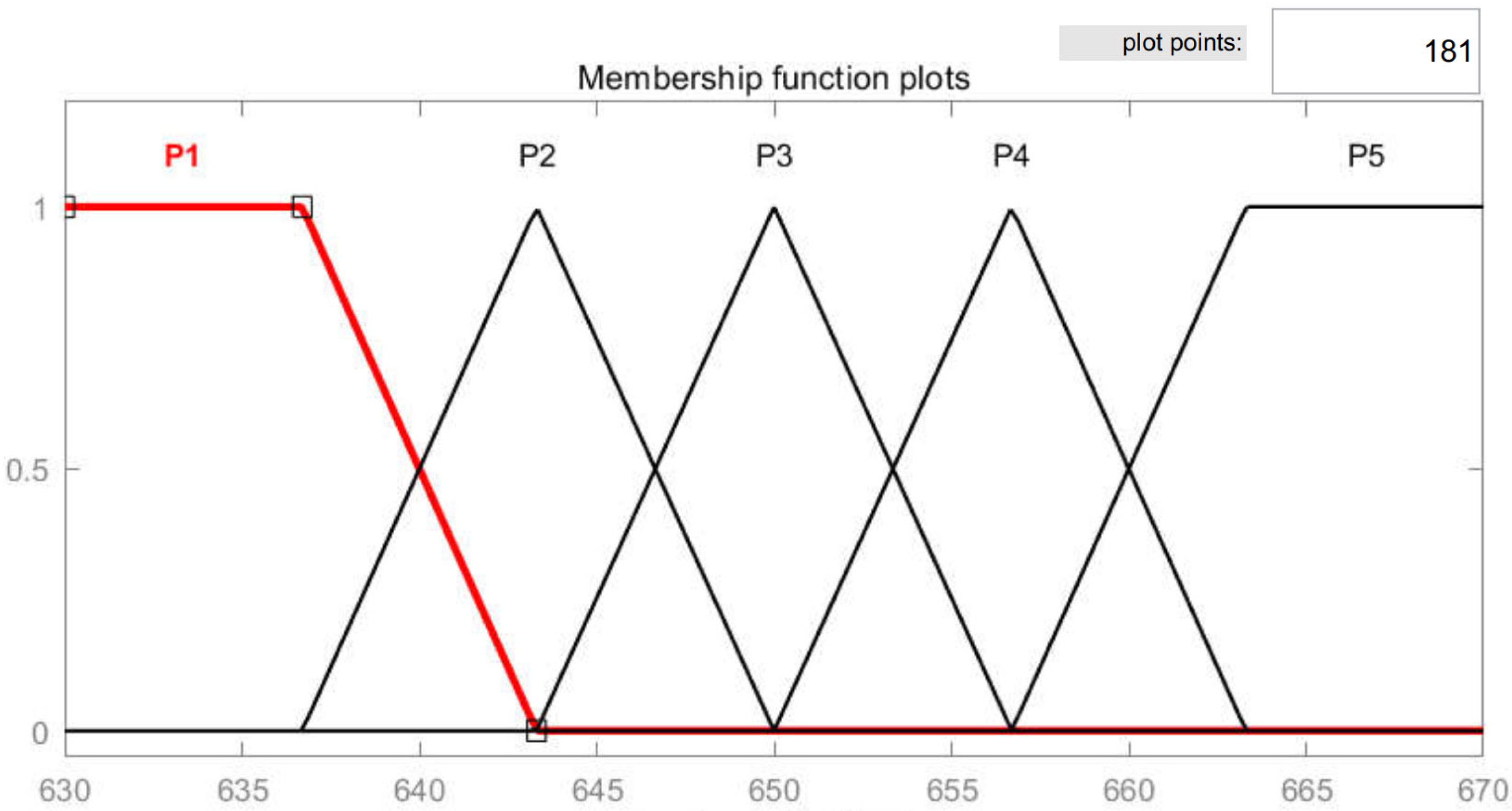
| DC bus voltage stability value/V | 650 |
| Initial droop coefficient of battery | 0.2 |
| Initial droop coefficient of super-capacitor | 0.2 |
Disclaimer/Publisher’s Note: The statements, opinions and data contained in all publications are solely those of the individual author(s) and contributor(s) and not of MDPI and/or the editor(s). MDPI and/or the editor(s) disclaim responsibility for any injury to people or property resulting from any ideas, methods, instructions or products referred to in the content. |
© 2024 by the authors. Licensee MDPI, Basel, Switzerland. This article is an open access article distributed under the terms and conditions of the Creative Commons Attribution (CC BY) license (https://creativecommons.org/licenses/by/4.0/).
Share and Cite
Wang, C.; Jiao, S.; Zhang, Y.; Wang, X.; Li, Y. Adaptive Variable Universe Fuzzy Droop Control Based on a Novel Multi-Strategy Harris Hawk Optimization Algorithm for a Direct Current Microgrid with Hybrid Energy Storage. Energies 2024, 17, 5296. https://doi.org/10.3390/en17215296
Wang C, Jiao S, Zhang Y, Wang X, Li Y. Adaptive Variable Universe Fuzzy Droop Control Based on a Novel Multi-Strategy Harris Hawk Optimization Algorithm for a Direct Current Microgrid with Hybrid Energy Storage. Energies. 2024; 17(21):5296. https://doi.org/10.3390/en17215296
Chicago/Turabian StyleWang, Chen, Shangbin Jiao, Youmin Zhang, Xiaohui Wang, and Yujun Li. 2024. "Adaptive Variable Universe Fuzzy Droop Control Based on a Novel Multi-Strategy Harris Hawk Optimization Algorithm for a Direct Current Microgrid with Hybrid Energy Storage" Energies 17, no. 21: 5296. https://doi.org/10.3390/en17215296
APA StyleWang, C., Jiao, S., Zhang, Y., Wang, X., & Li, Y. (2024). Adaptive Variable Universe Fuzzy Droop Control Based on a Novel Multi-Strategy Harris Hawk Optimization Algorithm for a Direct Current Microgrid with Hybrid Energy Storage. Energies, 17(21), 5296. https://doi.org/10.3390/en17215296