A Joint Estimation Method of Distribution Network Topology and Line Parameters Based on Power Flow Graph Convolutional Networks

Abstract

Accurate identification of network topology and line parameters is essential for effective management of distribution systems. An innovative joint estimation method for distribution network topology and line parameters is presented, utilizing a power flow graph convolutional network (PFGCN). This approach addresses the limitations of traditional methods that rely on costly voltage phase angle measurements. The node correlation principle is applied to construct a node correlation matrix, and a minimum distance iteration algorithm is proposed to generate candidate topologies, which serve as graph inputs for the parameter estimation model. Based on the topological dependencies and convolutional properties of AC power flow equations, a PFGCN model is designed for line parameter estimation. Parameter refinement is achieved through an alternating iterative process of pseudo-trend calculation and neural network training. Training convergence and loss function values are used as feedback to filter and validate candidate topologies, enabling precise joint estimation of both topologies and parameters. The proposed method’s accuracy, transferability, and robustness are demonstrated through experiments on the IEEE-33 and modified IEEE-69 distribution systems. Multiple metrics, including MAPE, IAE, MAE, and R², highlight the proposed method’s advantages over Adaptive Ridge Regression (ARR). In the C33 scenario, the proposed method achieves MAPEs of 4.6% for g and 5.7% for b, outperforming the ARR method with MAPEs of 7.1% and 7.9%, respectively. Similarly, in the IC69 scenario, the proposed method records MAPEs of 3.0% for g and 5.9% for b, surpassing the ARR method’s 5.1% and 8.3%.

1. Introduction

With the integration of new elements, such as distributed energy resources and energy storage systems, the structure of distribution networks has become increasingly complex. At the same time, user demand for electricity continues to grow. This development has raised requirements for the planning and management, safe operation, and condition monitoring of distribution networks [1,2]. Accurate topological information and line parameters are essential for efficient planning and operation of distribution systems. However, due to limited investment from distribution system operators, many networks lack the necessary monitoring equipment, resulting in low observability [3]. Additionally, sloppy management and untimely data updates during line reconstruction and maintenance have exacerbated the missing topological information and line parameters, making accurate estimation more challenging [3,4].

The continuous improvement of advanced metering infrastructure (AMI) has helped alleviate the observability issues in distribution systems. These infrastructures also provide a vast amount of measurement data, which serve as a solid foundation for the application of data-driven methods. As a result, data-driven methods have emerged as a prominent research focus in topology identification and parameter estimation for power distribution systems. These methods are primarily divided into modeling approaches and neural network-based techniques.

Depending on the study’s scope, the modeling methods can be further classified into single-attribute and joint-estimation approaches. Single-attribute approaches concentrate on either topology identification or line parameter estimation. Typically, topology identification relies on node correlations, whereas line parameter estimation is based on power flow equations. The literature [5] introduces a time-series signature verification method that detects topology changes in distribution networks by analyzing Phasor Measurement Unit (PMU) data characteristics. In [6], energy data are used to infer network topology through the law of energy conservation and principal component analysis. A graph recovery algorithm that identifies the topology using node voltage data is presented in [7]. In [8], a Markov Random Field approach is used to analyze node voltage correlations, and maximum likelihood estimation is employed to solve the topology. For real-time topology prediction, the literature [9] proposes a two-stage topology identification method based on split expectation maximization. However, this approach demands high data integrity. These topology identification studies generally rely on a single correlation analysis, making the results vulnerable to interference from specific factors. The literature [10] introduces a weighted least squares (WLS) method for line parameter estimation, while the literature [11] presents a weighted nonlinear least squares approach. However, both regression algorithms are susceptible to data errors, and their accuracy remains challenging. Additionally, methods based on voltage phase angle data ([5,9,10]) encounter significant obstacles in real-world distribution networks due to the limited coverage and high cost of PMU devices.

The simultaneous loss of topology and line parameter information is common in real distribution networks [2]. A joint estimation approach that concurrently addresses topology identification and line parameter estimation is better suited to practical applications. The literature [12] first recovers the network topology using a linear regression algorithm, followed by line parameter estimation from leaf to root nodes. The literature [1] uses a topology labeling matrix based on a linear power flow model to identify the topology through feature clustering, with line parameters estimated via linear regression. In [2], a linear power flow model is used to approximate resistive distances between nodes, and a recursive grouping algorithm is then applied to recover topology and estimate line impedance. The literature [13] deploys a small number of PMUs and iteratively solves topology and line parameters using a trace-free Kalman filter combined with the Newton–Raphson method. The literature [14,15] apply pseudo-trend and Newton–Raphson iterative techniques for joint topology and line parameter estimation. However, linear power flow models are often insufficiently accurate, and Newton–Raphson’s iterative convergence can be unstable and sensitive to initial conditions.

Neural networks offer significant advantages over traditional model-based methods in handling complex nonlinear relationships, which have garnered widespread attention. The literature [16] applies convolutional neural networks (CNNs) to the topology identification problem, while the literature [17] introduces a topology identification method for distribution networks using attentional and convolutional neural networks (ACNNs). The literature [18] leverages CNNs to extract PMU data features for constructing a line parameter identification model. However, these studies treat topology identification and line parameter estimation as classification or screening problems, limiting their applicability in distribution networks with missing topology information and line parameters. The literature [19] integrates graph convolutional networks and fully convolutional networks for parameter estimation in transmission grids, but this approach is unsuitable for distribution grids with limited measurement devices. The literature [20] presents a topology and parameter estimation method using deep and shallow neural networks; however, it requires partitioning the network into regions based on observability, which poses significant challenges in practical applications. The literature [21,22] demonstrated the feasibility of estimating line parameters via gradient descent by embedding distribution network topology into a graph neural network. Nevertheless, the neural networks in these studies lack explicit physical information and interpretability. Additionally, the advantages of graph neural networks in processing non-Euclidean data were only partially exploited.

This paper proposes a joint topology and parameter identification method for distribution networks to address these challenges using a Power Flow Graph Convolutional Network (PF-GCN). The approach integrates graph convolution theory with AC power flow equations to develop a novel PF-GCN with explicit physical information, which is then used to construct the parameter identification model. Additionally, an improved voltage correlation-based algorithm is applied for the joint identification of network topology and parameters. Given the high costs associated with PMU deployment, the proposed method bypasses the need for voltage phase angle data, relying solely on voltage magnitude and power data for accurate identification. The method’s effectiveness and accuracy advantage are validated through experiments on the IEEE 33-bus system and the modified IEEE-69 bus system. To summarize, the following contributions have been made in this paper:

(1)

This paper introduces a novel convolutional network for power flow, leveraging the topological dependencies and complex-valued convolution properties of AC power flow equations. The proposed network enhances line parameter identification accuracy and offers physical interpretability and adaptability to varying topologies.

(2)

The proposed topology identification method combines the dual correlation of node voltage magnitudes and their trends, ensuring strong robustness and improved identification accuracy.

(3)

This method relies solely on power and voltage magnitude data, eliminating the need for voltage phase angle measurements, which avoids the high costs of PMU deployment and greatly enhances practicality.

The rest of the paper is organized as follows: Section 2 presents the framework for joint estimation of topology and line parameters. Section 3 outlines the generation of candidate topologies, defines the node correlation matrix, and introduces a minimum distance iteration algorithm. Section 4 details the derivation of the principles behind the PF-GCN-based parameter estimation model and discusses the critical elements of network design. Section 5 presents experimental results for the IEEE-33 and improved IEEE-69 systems. Section 6 summarizes the conclusions of this paper.

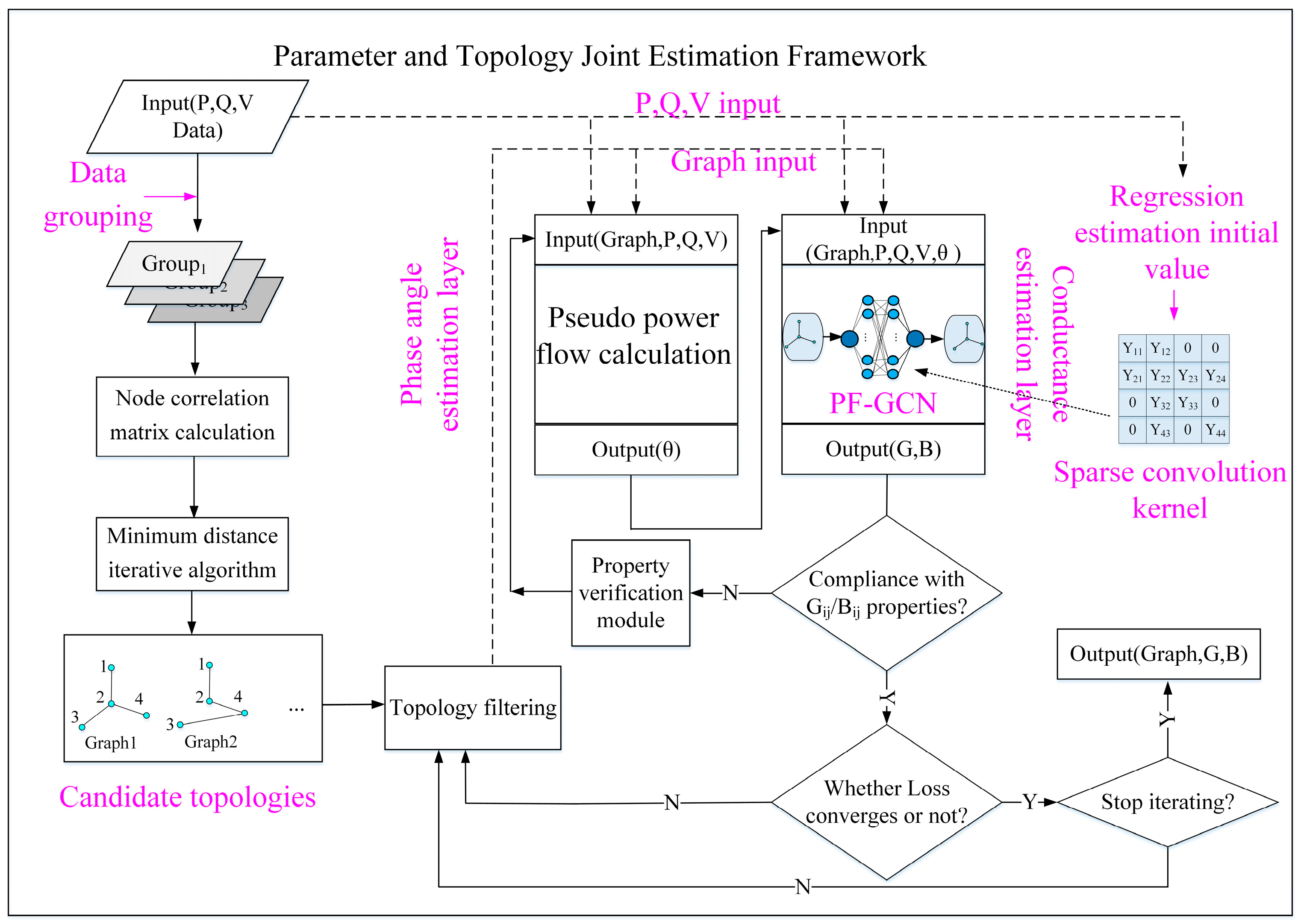
2. A Framework for Joint Estimation of Topology and Line Parameters

In this paper, we propose an innovative framework for the joint identification of topology and line parameters, as illustrated in Figure 1. The inputs to the framework are power and voltage magnitude measurements, which are grouped to reduce computational complexity and improve the fault tolerance of the topology identification process. Data grouping occurs only in the topology identification session.

The node correlation matrix is constructed by calculating the Euclidean Distance and Dynamic Time Warping (DTW) Distance between nodes. A minimum distance iterative algorithm is then applied to generate a set of candidate topologies. By constructing a set of candidate topologies rather than a single topology, the robustness of the topology identification is significantly enhanced. This candidate topology information is encoded in the node correlation matrix and serves as input to the graph structure for subsequent parameter estimation.

In this paper, the line parameter estimation is formulated as an optimization problem to minimize the power estimation error. Given the lack of voltage phase angle data in real-world measurements, we employ a pseudo power flow calculation method to estimate these values. An iterative mechanism is designed, consisting of a phase angle estimation layer and a conductance estimation layer, to accurately estimate the line parameters. This paper develops a power flow graph convolutional network (PFGCN) at the parameter estimation layer, which leverages the topological dependencies and complex-valued convolution properties of the AC power flow equations. Unlike traditional graph convolutional networks, PFGCN is an integrated model where neuron connections and operations directly correspond to AC power flow equations. In these equations, the network’s convolutional kernel is equivalent to the conductivity matrix. Importantly, PFGCN achieves parameter estimation through the training process.

The network provides strong interpretability by customizing filters that match the characteristics of the conductance matrix. The initial values of the convolution kernels are derived through linear estimation using power and voltage magnitude data. The graph input determines the size of the network’s convolution kernel, enabling the model to adapt to varying topologies. The topology identification step provides candidate topologies to the PF-GCN, creating a seamlessly integrated and adaptive system. The framework also incorporates a parameter matrix property verification module, which dynamically adjusts the convolutional kernel parameters during the iterative process to ensure that they meet the inherent properties of the conductance matrix. Additionally, the framework filters candidate topologies based on the final loss function value and its convergence behavior. Since the AC power flow equation is central to this framework, accurate topology and line parameters are crucial for achieving smaller loss function values. The iterative process sets an explicit termination condition. The iteration terminates when ${\displaystyle \frac{\left|F_i^n-F_i^{n-1}\right|}{F_i^n}}<=\xi$, $F_i^n$ represents the value of the loss function for the $nth$ iteration of group $i$.

3. Candidate Topology Generation

This section describes the definition of graphs and the principle of node correlation and defines the node correlation matrix and the minimum distance iteration algorithm.

3.1. Definition of Graphs and the Principle of Node Correlation

Graphs are nonlinear data structures used to describe non-Euclidean spatial relations. Low-voltage distribution networks usually exhibit a radial grid structure [7], and an undirected graph can represent their topology as $\widehat{G}=\left(V,B\right)$, where $V$ and $B$ denote the vertex set and edge set, respectively. The node adjacency matrix $A$ encodes and stores the undirected graph information, which is defined as:

$$\left\{\begin{array}{c}{a}_{ij}=1,if\mathrm{node}i,j\mathrm{have}\mathrm{a}\mathrm{connection}\\ a_{ij}=0,if\mathrm{node}i,j\mathrm{have}\mathrm{no}\mathrm{connection}\end{array}\right.$$

(1)

Taking the line shown in Figure 2 as an example, the voltage between node $i$ and node $i-1$ satisfies the following equation:

$${\stackrel{·}{V}}_{i-1}-{\stackrel{·}{V}}_i=\left(r_i+j{x}_i\right){\stackrel{·}{I}}_{i-1}=\left(r_i+j{x}_i\right){\stackrel{·}{I}}_i$$

(2)

Node voltage ${\stackrel{·}{V}}_i$ and line current ${\stackrel{·}{I}}_i$ are satisfied:

$$S_i={\dot{V}}_i{\dot{I}}_i^{\ast }=P_i+j{Q}_i$$

(3)

where ${\dot{I}}_i^{\ast }$ is the conjugate vector of ${\stackrel{·}{I}}_i$.

Bringing Equation (3) into Equation (2) gives the equation:

$${\stackrel{·}{V}}_{i-1}=\left(V_i+{\displaystyle \frac{P_i{r}_i+Q_i{x}_i}{V_i}}\right)+j{\displaystyle \frac{P_i{x}_i-Q_i{r}_i}{V_i}}$$

(4)

The voltage between any two nodes in the line is related to the load distribution and line parameters. As the physical distance between nodes decreases, the smaller the real and imaginary quantities of the voltage landings, the smaller the variability of the voltage amplitude at the exact moment, and the trend of the voltage changes at different moments are more similar [8].

3.2. Node Correlation Matrix Calculation

Curve correlation is assessed in two key dimensions: numerical values and change trends. As a standard metric, Euclidean distance quantifies the similarity between two curves by calculating the point-wise numerical distance between corresponding data points [23]. Dynamic Time Warping (DTW) is a widely used distance metric for time series data. Derivative dynamic time warping (DDTW) is a modified method of DTW, which alleviates the problem of pathological alignment. DDTW is computed using the first-order discrete derivatives of the original data, enabling better characterization of the trend changes in time series data [24,25]. Correlation estimation based solely on one dimension is susceptible to specific influences. Therefore, this paper integrates DDTW and Euclidean distance to capture node voltage correlations jointly.

Assume that the voltage data of the node $a,b$ are $V_a=[V_{a,1}{V}_{a,2}{V}_{a,3}\dots V_{a,m}],V_b=[V_{b,1}{V}_{b,2}{V}_{b,3}\dots V_{b,m}]$. The Euclidean distance between two nodes is:

$$d_{ab}^{ou}=\sqrt{{\displaystyle \sum _{i=1}^m{(V_{a,i}-V_{b,i})}^2}}$$

(5)

where $V_{a,i},V_{b,i}$ are the $ith$ elements in $V_a,V_b$, respectively; $m$ is the number of measurement groups.

The DDTW distance between nodes $a,b$ is:

$$d_{DDTW}(V_a,V_b)=\underset{C}{\min }\sqrt{{\displaystyle \sum _{s=1}^S{C}_s}}$$

(6)

where $C$ is the DDTW optimal path, $C=\left\{c_1,c_2,\dots ,c_p\right\}$; $S$ is the number of elements on the path.

The DDTW distance is calculated based on the first-order discrete derivative of the original data. The first-order discrete derivative of the original data is defined as:

$${V^{\prime }}_a=\left\{\begin{array}{c}{V}_{a,i}^{\prime }={\displaystyle \frac{(V_{a,i}-V_{a,i-1})+(V_{a,i+1}-V_{a,i-1})/2}{2}}2\le i<m\\ V_{a,i}^{\prime }=V_{a,2}-V_{a,1}\hspace{1em}\hspace{1em}\hspace{1em}\hspace{1em}i=1\\ \begin{array}{l}{V}_{a,i}^{\prime }=V_{a,m}-V_{a,m-1}\hspace{1em}\hspace{1em}\hspace{1em}\hspace{1em}i=m\end{array}\end{array}\right.$$

(7)

where ${V^{\prime }}_a$ is the first-order discrete derivative of the original data $V_a$; $m$ is the number of measurement groups.

The DDTW optimal path $C$ is built on a distance matrix consisting of ${V^{\prime }}_a,{V^{\prime }}_b$ with matrix elements $d\left(i,j\right)={\left({V^{\prime }}_{a,i}-{V^{\prime }}_{b,j}\right)}^2$. $(i,j)$ is the coordinate of the matrix. The optimal path satisfies the following conditions:

$$\left\{\begin{array}{c}{c}_1=d\left(1,1\right),c_p=d\left(p,p\right)\\ c_k=d\left(i_k,j_k\right),c_{k+1}=\left(i_{k+1},j_{k+1}\right)\\ i_{k+1}-i_k\le 1,j_{k+1}-j_k\le 1\\ i_k\le i_{k+1},j_k\le j_{k+1}\end{array}\right.$$

(8)

The Euclidean distance matrix $D={\left[d_{ij}^{ou}\right]}_{n\times n}$ and the DDTW distance matrix $T={\left[d_{ij}^{ddtw}\right]}_{n\times n}$ for the $n$-node system are calculated by Equations (5)–(8). The matrix is normalized using the following equation:

$$\left\{\begin{array}{c}{D}_{ij}^{\#}={\displaystyle \frac{d_{ij}^{ou}}{{\displaystyle \sum _{j=1}^n{d}_{ij}^{ou}}}}\\ T_{ij}^{\#}={\displaystyle \frac{d_{ij}^{ddtw}}{{\displaystyle \sum _{j=1}^n{d}_{ij}^{ddtw}}}}\end{array}\right.$$

(9)

where $n$ is the number of nodes; $D_{ij}^{\#},T_{ij}^{\#}$ are the normalized $D,T$, respectively.

After normalization, the node correlation matrix $K$ is constructed by:

$$K=\left[(1-\alpha )D_{ij}^{\#}+\alpha T_{ij}^{\#}\right]$$

(10)

where $\alpha$ is the combination coefficient. The main diagonal element of the node correlation matrix $K$ is 0, and the values of the remaining positional elements are inversely proportional to the correlation.

3.3. Minimum Distance Iteration Algorithm

The node correlation matrix $K$ encodes the connectivity relationships between nodes, where smaller element values indicate stronger correlations between the corresponding nodes. To identify the topological connectivity relationships from this matrix $K$, we propose a minimum distance iterative algorithm, as detailed in Algorithm 1, to extract these relationships and generate candidate topologies.

Algorithm 1: Minimum Node Distance Iterative Algorithm

Input: Correlation Matrix $K$ for U nodes

Output: Node adjacency matrix $A$

1:Initialize node pool $V$ = [0, 1, .., U − 1];Initialize line pool $B$ = []; Initialize node adjacency matrix $A\in R^{\mathrm{U}\times \mathrm{U}}$, all elements $a_{ij}$ = 0

2.Sort matrix $K$ in ascending order of rows to obtain an index matrix $M$

3.Traverse matrix $M$:

4.     If $M_{i1}=M_{j0}$ and $M_{i0}=M_{j1}$:

5.        Establish a connection between node i and node j, update $B$

6.     If $M_{i2}=M_{j2}$:

7.        Establish a connection for $M_{i2}$’s corresponding node based on the minimum distance, update $B$

8.Remove nodes in $B$ from $V$

9.While ($V$ > 0):

10.        Traverse $V$$,k=v_i$, establish a connection between node k and $M_{k1}$’s corresponding node, update $B$, remove nodes in $B$ from $V$

11. Update $A$ by $B$, return $A$

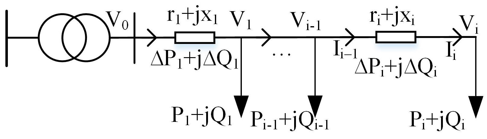
4. Line Parameter Estimation Model Based on PF-GCN

This section describes the theoretical foundation of Complex-Valued Graph Convolutional Network (CV-GCN), the principle derivation of the line parameter estimation model of PF-GCN, the network layer’s design, and the iterative initial value calculation.

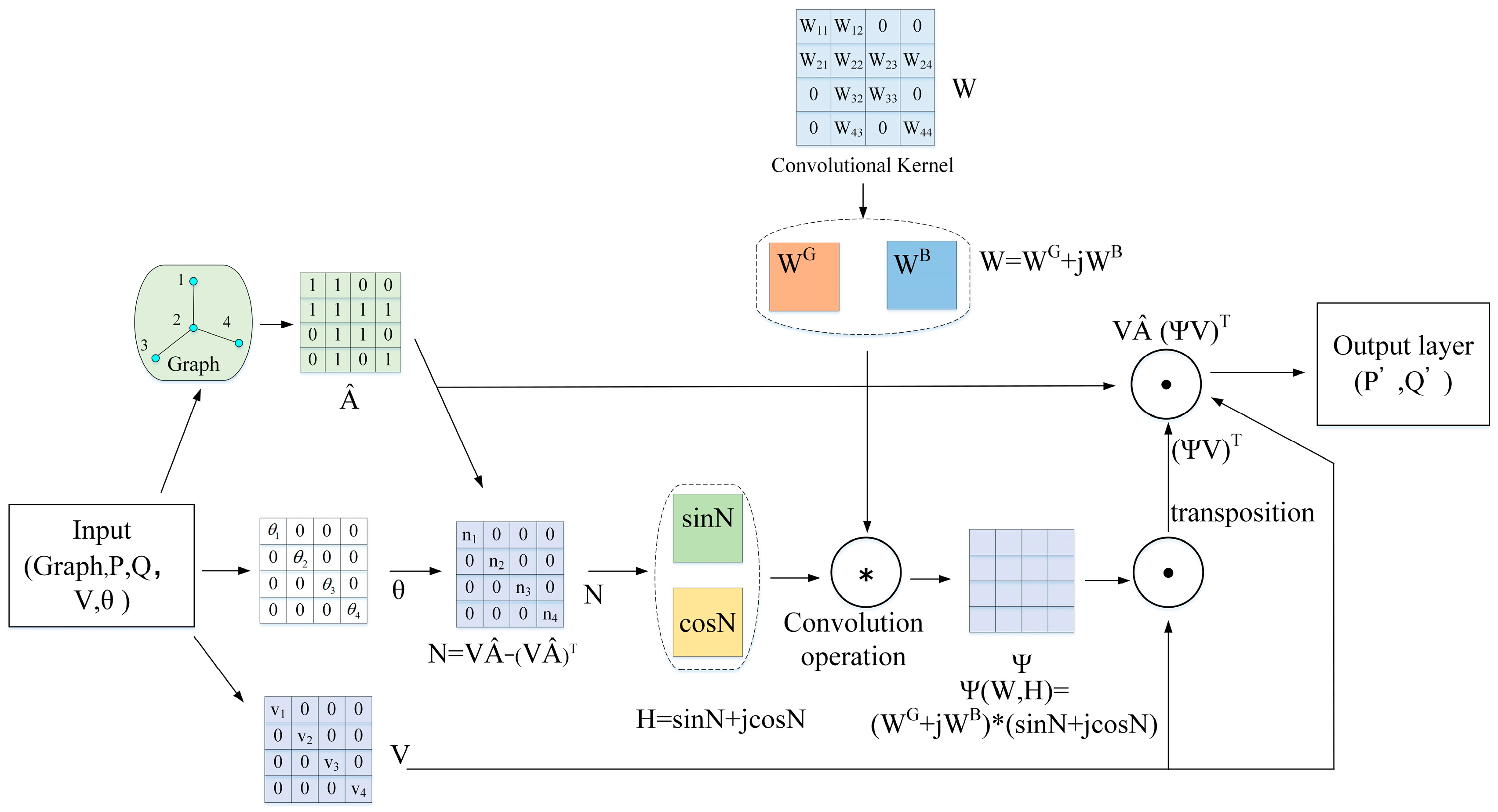
4.1. Theoretical Foundations of CV-GCN

The Graph Convolutional Network (GCN) [26] is a deep learning algorithm designed for graph-structured data. Its core concept is to extract and integrate both local features of nodes and their neighboring nodes, as well as global features, by applying convolution operations on the graph’s adjacency matrix. The forward propagation formula is:

$$H^{\left(l+1\right)}=\sigma \left({\widehat{D}}^{-{\displaystyle \frac{1}{2}}}\widehat{A}{\widehat{D}}^{-{\displaystyle \frac{1}{2}}}{H}^{\left(l\right)}{W}^{\left(l\right)}\right)$$

(11)

where $H^{\left(l\right)}$ denotes the node feature matrix of the $l$th layer, and $H^{\left(l+1\right)}$ is the node feature matrix of the next layer; $\widehat{A}=A+I$ denotes the adjacency matrix $A$ of the graph plus the unit matrix $I$, and $\widehat{A}$ is the adjacency matrix considering the node self-loop; $\widehat{D}$ is $\widehat{A}$’s degree matrix, and ${\widehat{D}}_{ii}={\displaystyle \sum _j{\widehat{A}}_{ij}}$, denotes the number of edges connected by the $i$th node; $W^{\left(l\right)}$ is the $l$th layer trainable weight matrix; $\sigma \left(·\right)$ is the activation function.

A Complex-Valued Graph Convolutional Network (CV-GCN) extends this convolution operation from the real domain to the complex domain. This extension enables CV-GCN to effectively model complex signals by processing graph-structured data that include magnitude and phase information through complex-valued convolution operations [27]. The forward propagation formula is:

$$H^{\left(l+1\right)}=\sigma \left(\begin{array}{l}{\widehat{D}}^{-{\displaystyle \frac{1}{2}}}\widehat{A}{\widehat{D}}^{-{\displaystyle \frac{1}{2}}}\left(H_r^{\left(l\right)}{W}_r^{\left(l\right)}-H_i^{\left(l\right)}{W}_i^{\left(l\right)}\right)\\ +j{\widehat{D}}^{-{\displaystyle \frac{1}{2}}}\widehat{A}{\widehat{D}}^{-{\displaystyle \frac{1}{2}}}(H_r^{\left(l\right)}{W}_i^{\left(l\right)}+H_i^{\left(l\right)}{W}_r^{\left(l\right)})\end{array}\right)$$

(12)

Unlike traditional GCN, in CV-GCN, $H^{\left(l\right)}$ and $W^{\left(l\right)}$ are complex-valued matrices. $H^{\left(l\right)}=H_r^{\left(l\right)}+j{H}_i^{\left(l\right)},W^{\left(l\right)}=W_r^{\left(l\right)}+j{W}_i^{\left(l\right)}$, where subscripts $r$ and $i$ denote the real and imaginary parts, respectively.

4.2. Principles and Framework of PF-GCN Parameter Estimation Models

The basic principle of line parameter estimation is the AC power flow equation:

$$\left\{\begin{array}{c}{p}_i={\displaystyle \sum _{j=1}^n{v}_i{v}_j(G_{ij}\cos {\theta }_{ij}+B_{ij}\sin {\theta }_{ij})}\\ q_i={\displaystyle \sum _{j=1}^n{v}_i{v}_j(G_{ij}\sin {\theta }_{ij}-B_{ij}\cos {\theta }_{ij})}\end{array}\right.$$

(13)

where $p_i,q_i,v_i$ are the active power injection, reactive power injection, and voltage magnitude of the node $i$, respectively; $G_{ij},B_{ij}$ are the conductance of the line; ${\theta }_{ij}$ is the node phase angle discrepancy.

The AC power flow equations exhibit topological dependence, meaning that the power at any node is influenced not only by its state but also by the states of its neighboring nodes. Traditional parameter identification methods often struggle to effectively capture and utilize this topological interdependence, particularly in complex grid structures. Therefore, developing a method that efficiently integrates grid topology information is crucial.

The complex-valued characteristics of the AC power flow equations arise from the fact that electrical quantities, such as voltage, line parameters, and power, can be represented in complex form. A Complex-Valued Graph Convolutional Network (CV-GCN) offers exceptional capabilities for processing graph-structured data and handling complex-domain features, making it an optimal choice for aggregating node data features based on grid topology.

The process of mapping AC power flow equations into the complex-valued graph convolutional framework is as follows: the distribution network topology is encoded as a node adjacency matrix, voltage magnitudes, and phase angles are represented as diagonal matrices, and line parameters are expressed in the complex form using the conductance matrix. The following preprocessing is performed:

$$\left\{\begin{array}{c}\widehat{A}=A+I\\ N=diag({\theta }_i)\widehat{A}-{\left(diag({\theta }_i)\widehat{A}\right)}^T\\ Y_{ij}=G_{ij}+j{B}_{ij}\end{array}\right.$$

(14)

where $A$ is the node topology correlation matrix; $\widehat{A}$ is the node correlation matrix considering the self-loop; $I$ is the unit matrices; $diag({\theta }_i)$ is the diagonal array of the phase angle of the node voltages, with the head transformer node as the reference node by default; $G,B$ are the conductance and the conductivity matrices, respectively.

Define the following intermediate variable functions:

$$\left\{\begin{array}{c}\mathsf{\Phi }(G,B,N)=G\odot \cos N+B\odot \sin N\\ \mathsf{\Gamma }(G,B,N)=G\odot \sin N-B\odot \cos N\end{array}\right.$$

(15)

where $\mathsf{\Phi }(G,B,N)$ and $\mathsf{\Gamma }(G,B,N)$ are defined functions of the intermediate variables; the symbol $\odot$ denotes the Hadamard product; $\cos N,\sin N$ denote the cosine and sine of each element of the matrix $N$.

Bringing Equations (14) and (15) into Equation (13):

$$\left\{\begin{array}{c}P=diag(v_i)\widehat{A}{\left[\mathsf{\Phi }(G,B,N)diag(v_i)\right]}^T\odot I_n{I}_{n\times 1}\\ Q=diag(v_i)\widehat{A}{\left[\mathsf{\Gamma }(G,B,N)diag(v_i)\right]}^T\odot I_n{I}_{n\times 1}\end{array}\right.$$

(16)

where $I_{n\times n},I_{n\times 1}$ are the unit matrices; $diag(v_i)$ is the diagonal matrix of node voltage magnitudes; $P={\left[\begin{array}{cccc}{p}_1& p_2& \dots & p_n\end{array}\right]}^T$,$Q={\left[\begin{array}{cccc}{q}_1& q_2& \dots & q_n\end{array}\right]}^T$.

Equation (16) can be further combined to obtain the AC power flow equation in complex-valued convolution form as:

$$\left\{\begin{array}{c}\begin{array}{c}H=\sin N+j\cos N\\ Y=G+jB\end{array}\\ \mathsf{\Psi }(Y,H)=j(G\odot \cos N+B\odot \sin N)+(G\odot \sin N-B\odot \cos N)\\ Q+Pj=diag(v_i)\widehat{A}{\left[\mathsf{\Psi }(Y,H)diag(v_i)\right]}^T\odot I_n{I}_{n\times 1}\end{array}\right.$$

(17)

In the AC power flow equations, a node’s power data are influenced by its state and the states of its neighboring nodes. Therefore, constructing a Graph Convolutional Network (GCN) that aggregates features from a node and its first-order neighbors can effectively meet the data feature extraction requirements.

Given the high cost of obtaining voltage phase angle data in real-world distribution networks, this method deliberately avoids relying on such measurements. However, the absence of voltage phase angle information may negatively impact the accuracy of line parameter estimation. Fortunately, when the line parameters are known, pseudo-trend calculations can effectively estimate the missing voltage phase angle data [14,15]. Therefore, this study employs the pseudo-trend flow calculation method to supplement the required voltage phase angle information, ensuring accurate parameter estimation.

In summary, we designed a line parameter estimation model that includes both a phase angle estimation layer and a parameter estimation layer. The framework of this model is illustrated in Figure 3. The phase angle estimation layer estimates the voltage phase angle for a given line parameter through pseudo-current calculations. The results from the topology identification are used as graph inputs for the line parameter estimation model. The line parameter estimation layer then completes estimating line parameters using voltage magnitude, estimated voltage phase angle data, and power measurements. We formulate the line parameter estimation as an optimization problem to minimize power estimation error [14,15]. Its objective function is:

$$Min\left\{F\right\}=\underset{g,b,\theta }{Min}\left\{{\displaystyle \frac{1}{n}}\left({\displaystyle \sum _{i=1}^n{\left(p_i-p_i^{\prime }\right)}^2}+{{\displaystyle \sum _{i=1}^n\left(q_i-q_i^{\prime }\right)}}^2\right)\right\}$$

(18)

where $p_i,q_i$ are active and reactive power measurements of node $i$; $p_i^{\prime },q_i^{\prime }$ are active and reactive power estimates of node $i$.

Line parameter estimation is performed iteratively by estimating the voltage phase angle and line parameters, specifically through alternating the training of $f\left(v,G,B\right)\stackrel{\theta }{\to }\left\{P,Q\right\}$ and $f\left(v,\theta \right)\stackrel{G,B}{\to }\left\{P,Q\right\}$. It is essential to highlight that the line parameter estimation layer comprises a power flow graph convolutional network, a novel architecture that integrates graph convolution theory with AC power flow equations. The neurons and connections in this network correspond to the computational processes of the AC power flow equations, and the line parameters to be estimated are represented as sparse convolutional kernels. Unlike conventional convolutional neural networks, the power flow graph convolutional network optimizes its convolutional kernels for line parameter estimation through gradient descent [21] during training.

Figure 4 illustrates the architecture of the power flow graph convolutional network (PFGCN). In contrast to traditional graph convolutional networks, the PFGCN adopts a more integrated structure. Similar to conventional GCNs, the PFGCN layer utilizes node features while integrating external inputs that represent topological information encoded in the form of a node adjacency matrix with self-loops. In the parameter estimation layer, the input features for each node include voltage magnitude and power measurements. A vital aspect of this design is that the convolutional kernel used in the parameter estimation layer is tailored to the structure of the conductance matrix, with non-zero entries that align with the positions in the conductance matrix and share the same dimensionality [22]. As discussed in this paper, the conductance matrix for line parameters corresponds to the convolutional kernel in the parameter estimation layer. They represent the same concept but are described using different power systems and neural network terminologies.

To ensure that the convolutional kernel maintains the properties of the conductance matrix during training, a verification module is incorporated. This module checks for key properties such as row sums and column sums equal to zero, as well as the sign (positive or negative) of individual elements. If errors in the sign of the elements are detected, they are corrected using random numbers of the same magnitude. After correcting the row and column sums, the kernel is retrained to preserve accuracy.

The joint estimation of topology and line parameters is achieved through a topology correction phase. In this phase, the convergence of the parameter estimation process and the value of the loss function serve as signals for topology refinement. Ultimately, this process outputs the topology and its corresponding line parameters for which the training loss is converged and minimized.

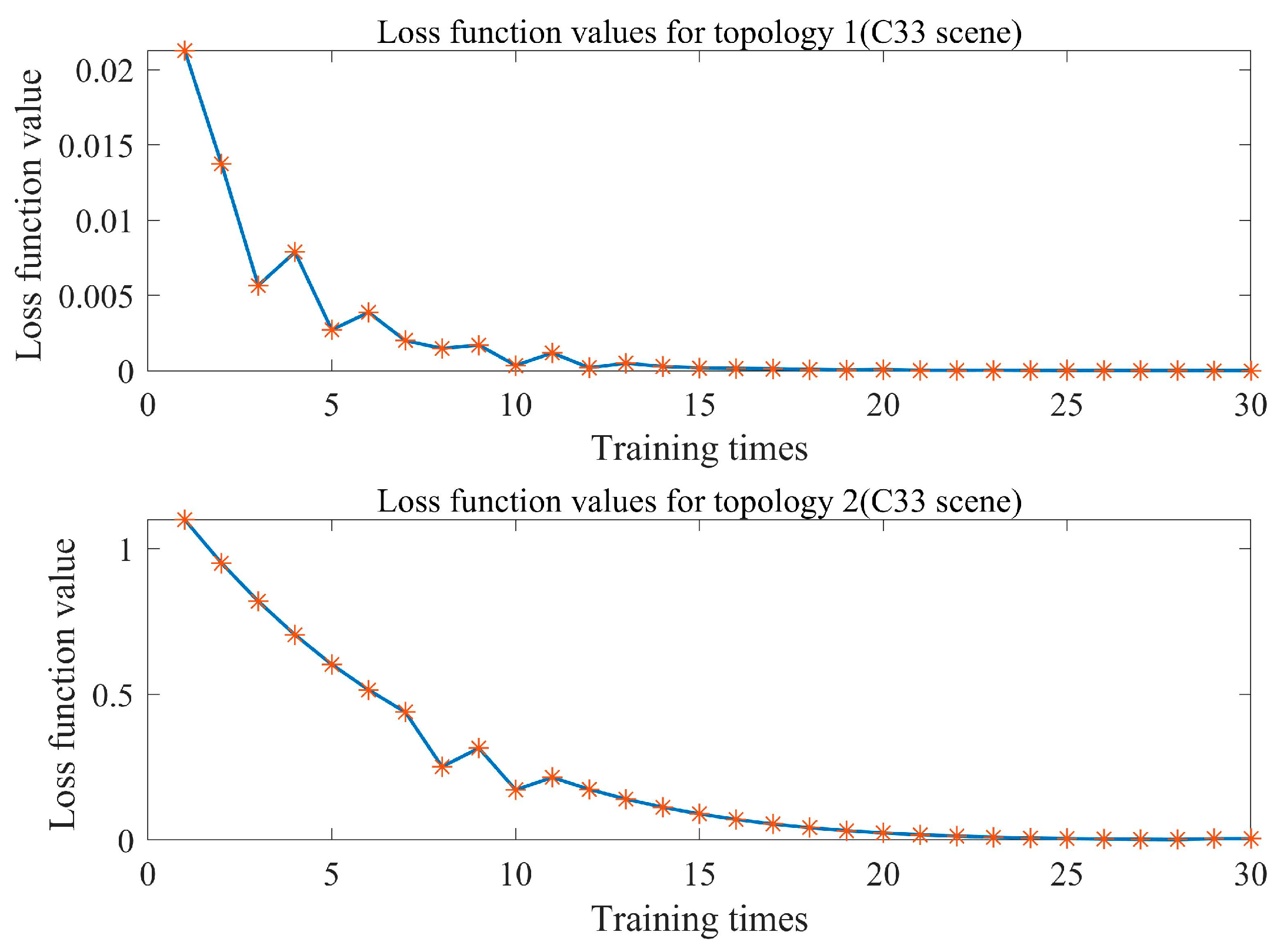
4.3. Loss Function Design for Parameter Estimation Layer

The inputs to the parameter estimation layer are topology, power, voltage magnitude data, and phase angle data from pseudo-trend estimation. The training objective is to minimize the error in active and reactive power estimation. Line parameter estimation is accomplished through a convolutional kernel designed to reflect the properties of the conductance matrix, enabling the network to learn and aggregate the features of neighboring nodes in the distribution network. The forward propagation in the line parameter estimation layer is formulated as follows:

$$h^{\left(l\right)}=diag\left(v_i\right)\widehat{A}{\left[\left(W\ast h^{\left(l-1\right)}\right)diag\left(v_i\right)\right]}^{\mathrm{T}}\ast I_{n\times n}{I}_{n\times 1}$$

(19)

where $h^{\left(l\right)},h^{\left(l-1\right)}$ are the outputs and inputs of the layer $l$, respectively; $I_{n\times n},I_{n\times 1}$ are mainly used for matrix transformations; $W$ is the convolution kernel; $\widehat{A}$ is the node topological adjacency matrix considering self-loops.

To constrain the numerical properties of the convolution kernel, the sum of rows, and the sum of columns to zero, we design and apply the following loss function:

$$\begin{array}{l}loss={\displaystyle \frac{1}{n}}\left({\displaystyle \sum _{i=1}^n{\left(p_i-{p^{\prime }}_i\right)}^2}+{{\displaystyle \sum _{i=1}^n\left(q_i-{q^{\prime }}_i\right)}}^2\right)+\\ {\displaystyle \frac{1}{n}}{\displaystyle \sum _{i=1}^n\left({\left({\displaystyle \sum _{j=1}^n{W}_{ij}^G}\right)}^2+{\left({\displaystyle \sum _{j=1}^n{W}_{ij}^B}\right)}^2\right)}+{\displaystyle \frac{1}{n}}{\displaystyle \sum _{j=1}^n\left({\left({\displaystyle \sum _{i=1}^n{W}_{ij}^G}\right)}^2+{\left({\displaystyle \sum _{i=1}^n{W}_{ij}^B}\right)}^2\right)}\end{array}$$

(20)

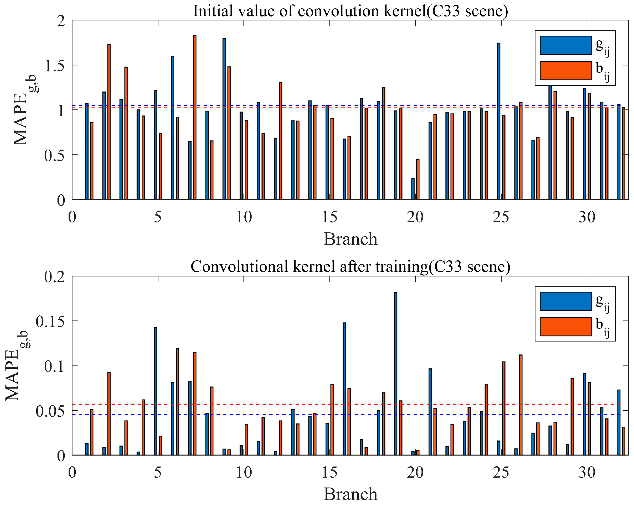
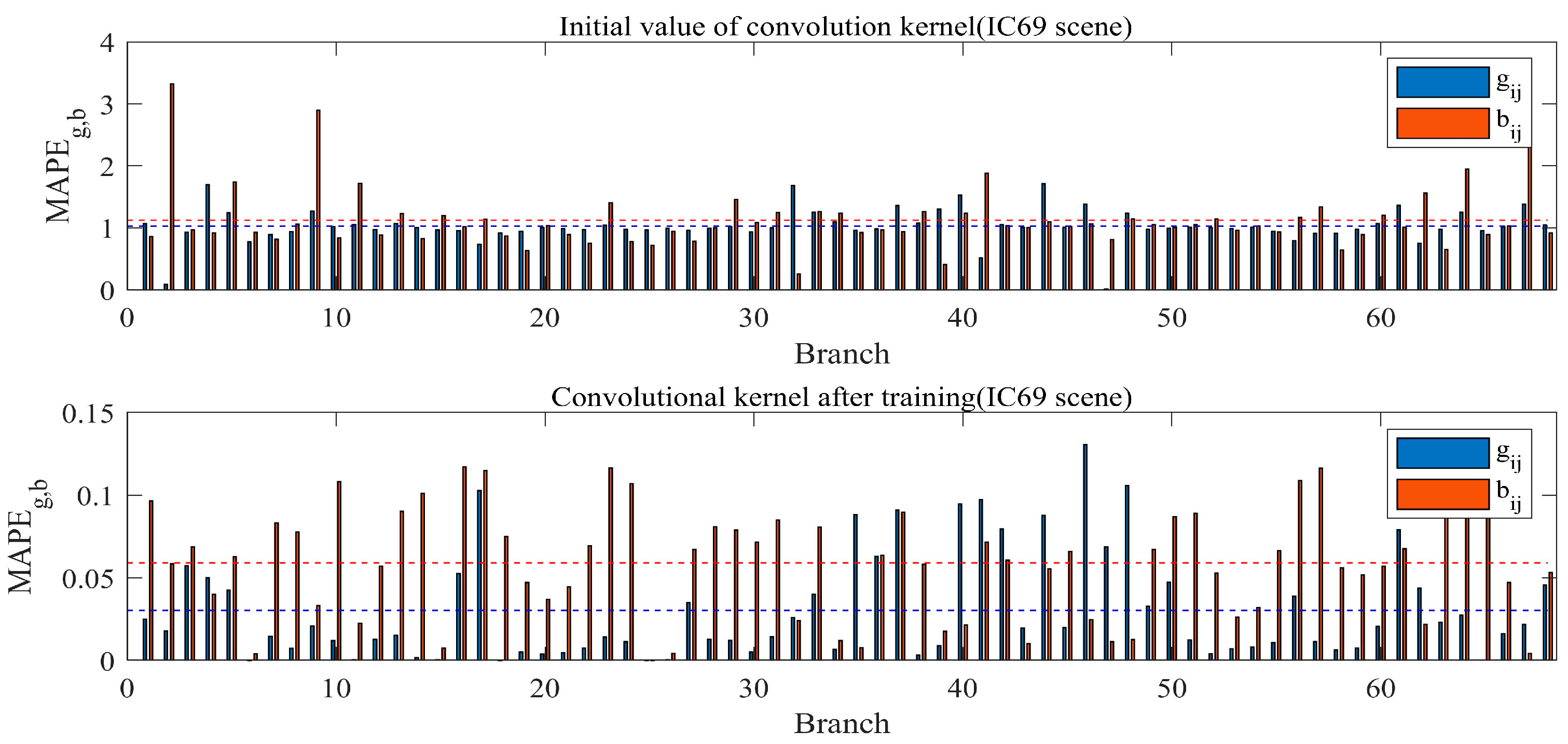
4.4. Convolution Kernel Iteration Initial Value Calculation

The operation of CV-GCN for line parameter estimation requires initial values for the convolution kernel. Selecting appropriate initial values can significantly accelerate convergence and enhance computational efficiency. Previous studies have demonstrated that line parameters estimated using linear regression methods provide valid estimates [14]. This work uses the regression-estimated line parameter values as the initial values for iterating the convolution kernel. During normal operation of a distribution network, the phase angle difference between the voltages of neighboring nodes is usually within $5^{\circ }$, so $\cos \theta \approx 1,\sin \theta \approx \theta$. The AC power flow equation (Equation (9)) can be rewritten as:

$$\left\{\begin{array}{c}{\displaystyle \frac{p}{v}}=\left[G_{ij}+{\theta }_{ij}{B}_{ij}\right]v\\ {\displaystyle \frac{q}{v}}=-\left[B_{ij}-{\theta }_{ij}{G}_{ij}\right]v\end{array}\right.$$

(21)

where ${\displaystyle \frac{p}{v}}={\left[\begin{array}{cccc}{\displaystyle \frac{p_1}{v_1}}& {\displaystyle \frac{p_2}{v_2}}& \dots & {\displaystyle \frac{p_n}{v_n}}\end{array}\right]}^T$; ${\displaystyle \frac{q}{v}}={\left[\begin{array}{cccc}{\displaystyle \frac{q_1}{v_1}}& {\displaystyle \frac{q_2}{v_2}}& \dots & {\displaystyle \frac{q_n}{v_n}}\end{array}\right]}^T$; $v={\left[\begin{array}{cccc}{v}_1& v_2& \dots & v_n\end{array}\right]}^T$; ${\theta }_{ij}={\theta }_i-{\theta }_j$.

Neglecting further the effect of the phase angle difference, the $m$-group voltage magnitude and power measurements satisfy the following equations:

$$\left\{\begin{array}{c}\left[{\displaystyle \frac{P}{V}}\right]=G_{ij}^{\prime }\left[\Delta V\right]\\ \left[{\displaystyle \frac{Q}{V}}\right]=-B_{ij}^{\prime }\left[\Delta V\right]\end{array}\right.$$

(22)

where $\left[{\displaystyle \frac{P}{V}}\right]=\left[\begin{array}{ccc}{\left[{\displaystyle \frac{p}{v}}\right]}_1& \dots & {\left[{\displaystyle \frac{p}{v}}\right]}_m\end{array}\right]$; $\left[{\displaystyle \frac{Q}{V}}\right]=\left[\begin{array}{ccc}{\left[{\displaystyle \frac{q}{v}}\right]}_1& \dots & {\left[{\displaystyle \frac{q}{v}}\right]}_m\end{array}\right]$; $\left[V\right]=\left[\begin{array}{ccc}{\left[v\right]}_1& \dots & {\left[v\right]}_m\end{array}\right]$.

The $G_{ij}^{\prime },B_{ij}^{\prime }$ obtained based on regression estimation is valuable as a rough estimate of $G_{ij},B_{ij}$ [14]. The equation for the regression estimation is:

$$\left\{\begin{array}{c}{G}_{ij}^{\prime }=\left[P/V\right]{\left[\Delta V\right]}^T{(\left[\Delta V\right]{\left[\Delta V\right]}^T)}^{-1}\\ B_{ij}^{\prime }=-\left[Q/V\right]{\left[\Delta V\right]}^T{(\left[\Delta V\right]{\left[\Delta V\right]}^T)}^{-1}\end{array}\right.$$

(23)

The regression estimates $G_{ij}^{\prime },B_{ij}^{\prime }$ are often non-sparse matrices, and we use the regression estimates as convolution kernel initial values after correcting them by the derivative matrix property.

5. Results

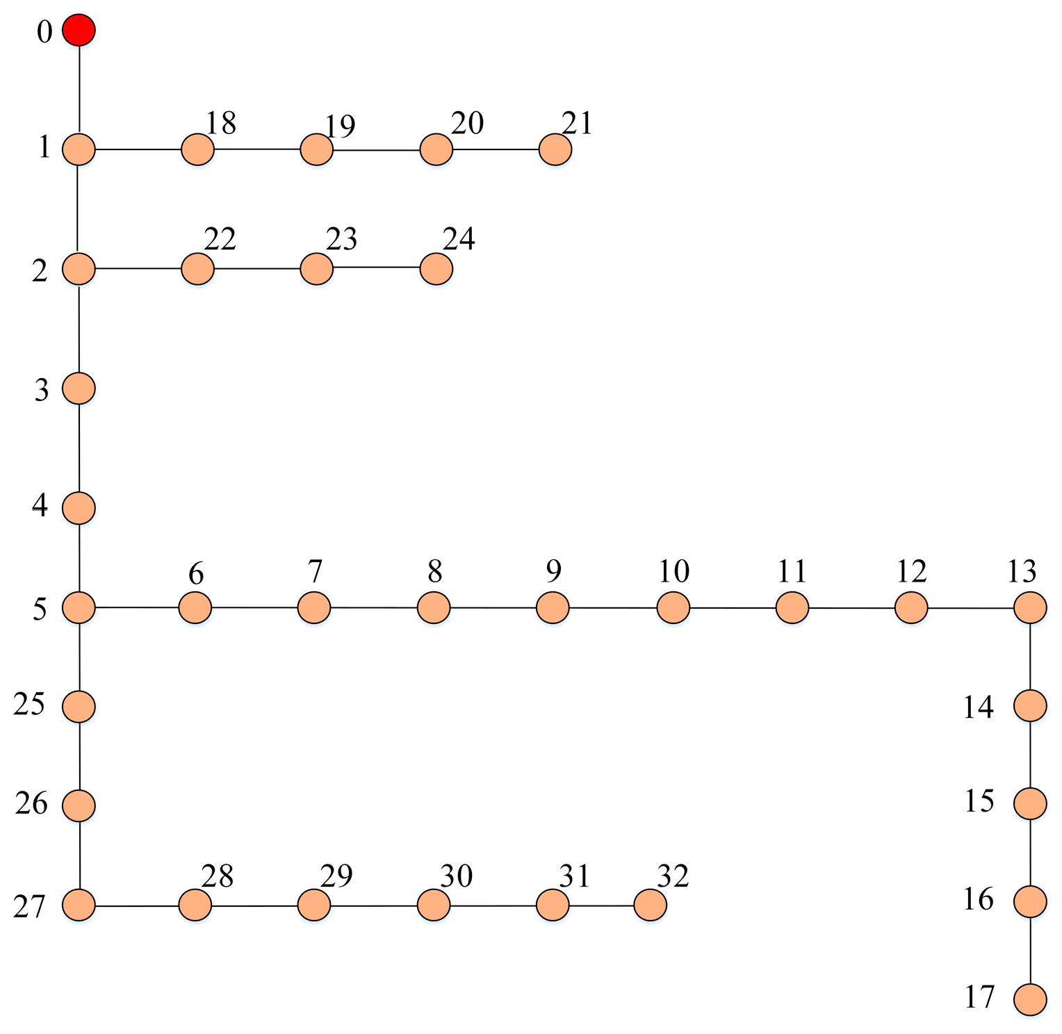
5.1. Introduction to Experiments

We evaluated the performance of the proposed algorithm on both the IEEE-33 node system and the modified IEEE-69 node system, as shown in Figure 5 and Figure 6. The node loads were randomly assigned based on historical load data from real distribution networks in Sichuan Province. Missing voltage magnitude data were imputed using MATPOWER7.1 [13]. In both test systems, the first node was designated as the transformer node, assuming that all nodes’ voltage magnitude and load data were fully accessible and the system topology remained unchanged throughout the sampling period without any data loss.

For each test system, we simulated 600 sets of ideal voltage magnitude and power measurements (random error $\epsilon$ = 0) to validate the methodology’s accuracy and scalability. The data were grouped based on empirical values, with each group comprising 100 sampling points, closely matching the real-world distribution system, which typically collects 96 data points per day. Additionally, experiments involving random sampling errors were conducted to approximate real-world conditions, as discussed in the error sensitivity analysis section. The PFGCN network proposed in this paper differs from the traditional GCN, which completes the corresponding tasks during the training process, so there is no need to differentiate between the training and validation sets. We take 600 sets of simulated data as the training set. The scenes are set up as follows:

• C33: IEEE-33 system, 600 measurements, random error $\epsilon$ = 0;
• IC69: Improved IEEE-69 system, 600 measurements, random error $\epsilon$ = 0.

5.2. Evaluation Indicators

The topological information in the method proposed in this paper is encoded in the node association matrix, and the topological accuracy function is defined as follows:

$$A_1\left(A,E\right)={\displaystyle \frac{1}{n^2}}{\displaystyle \sum _{i=1}^n{\displaystyle \sum _{j=1}^n\left|A_{ij}\cap E_{ij}\right|}}$$

(24)

where $n$ is the number of nodes; $A,E$ is the candidate topological node association matrix and the actual topological node association matrix, respectively. $A_1$ indicates the proportion of correct lines in the identification results, and the closer its value is to 1, the higher the accuracy of topology identification.

The parameter identification results in line conductance $g,b$, and we used Mean Absolute Percentage Error (MAPE) as the main evaluation metric to assess the effectiveness of parameter estimation. Small MAPE values imply high accuracy in parameter identification. MAPE is calculated as:

$$\left\{\begin{array}{c}MAP{E}_g={\displaystyle \frac{100\%}{N_b}}{\displaystyle \sum _{i=1}^{N_b}\left|\frac{g_i^{\prime }-g_i}{g_i}\right|}\\ MAP{E}_b={\displaystyle \frac{100\%}{N_b}}{\displaystyle \sum _{i=1}^{N_b}\left|\frac{b_i^{\prime }-b_i}{b_i}\right|}\end{array}\right.$$

(25)

where $N_b$ is the number of lines; $g_i^{\prime },b_i^{\prime }$ are the estimated value of line parameters; $g_i,b_i$ are the reference value of line parameters.

Additionally, we incorporate other evaluation metrics, including Integral Absolute Error (IAE), Mean Absolute Error (MAE), and the Coefficient of Determination (R²). These metrics offer a more comprehensive perspective for evaluating and comparing algorithm performance. The integral absolute error (IAE) is calculated as:

$$\left\{\begin{array}{c}IA{E}_g={\displaystyle \sum _{i=1}^{N_b}\left|g_i^{\prime }-g_i\right|}\\ IA{E}_b={\displaystyle \sum _{i=1}^{N_b}\left|b_i^{\prime }-b_i\right|}\end{array}\right.$$

(26)

The mean absolute error (MAE) is calculated as:

$$\left\{\begin{array}{c}MA{E}_g={\displaystyle \frac{1}{N_b}}{\displaystyle \sum _{i=1}^{N_b}\left|g_i^{\prime }-g_i\right|}\\ MA{E}_b={\displaystyle \frac{1}{N_b}}{\displaystyle \sum _{i=1}^{N_b}\left|b_i^{\prime }-b_i\right|}\end{array}\right.$$

(27)

The coefficient of determination (R²) is calculated as:

$$\left\{\begin{array}{c}{R}_g^2=1-{\displaystyle \frac{{\displaystyle \sum _{i=1}^{N_b}{\left(g_i-g_i^{\prime }\right)}^2}}{{\displaystyle \sum _{i=1}^{N_b}{\left(g_i-{\overline{g}}_i\right)}^2}}}\\ R_b^2=1-{\displaystyle \frac{{\displaystyle \sum _{i=1}^{N_b}{\left(b_i-b_i^{\prime }\right)}^2}}{{\displaystyle \sum _{i=1}^{N_b}{\left(b_i-{\overline{b}}_i\right)}^2}}}\end{array}\right.$$

(28)

5.3. IEEE-33 System Test Results

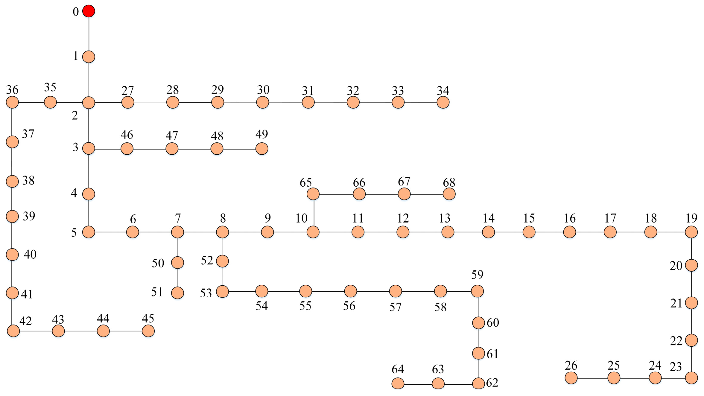
5.3.1. Candidate Topology Identification Results

In this subsection, we validate the topology recognition algorithm in scene C33. The data grouping is set to be 6, and the combination coefficient ${\alpha }_1$ of the matrix $K$ is set to be 0.6 (${\alpha }_1$ = 0.6). Data grouping reduces the matrix’s computational complexity and increases the topology identification algorithm’s robustness. The number of data groups is empirically determined according to the temporal order.

Figure 7 presents the results of the node correlation matrix calculation for the six data sets of scenario C33. The values of the correlation matrix elements are inversely proportional to the correlation between the corresponding indexed nodes. The experimental results demonstrate that the distribution of the correlation matrix data aligns, to some extent, with the topology of the IEEE-33 system. This finding confirms that the node correlation matrix defined in this paper effectively captures and represents the correlation between nodes.

Table 1. C33 scene, ${\alpha }_1$ = 0.6, candidate topology results.

Group	1	2	3	4	5	6
$A_1$	1	1	1	0.9963	1	0.9963

shows the results of the minimum distance iteration algorithm for candidate topology identification in scenario C33. The candidate topology set, consisting of six topology groups, includes the correct topology. This confirms the effectiveness of the proposed candidate topology identification method.

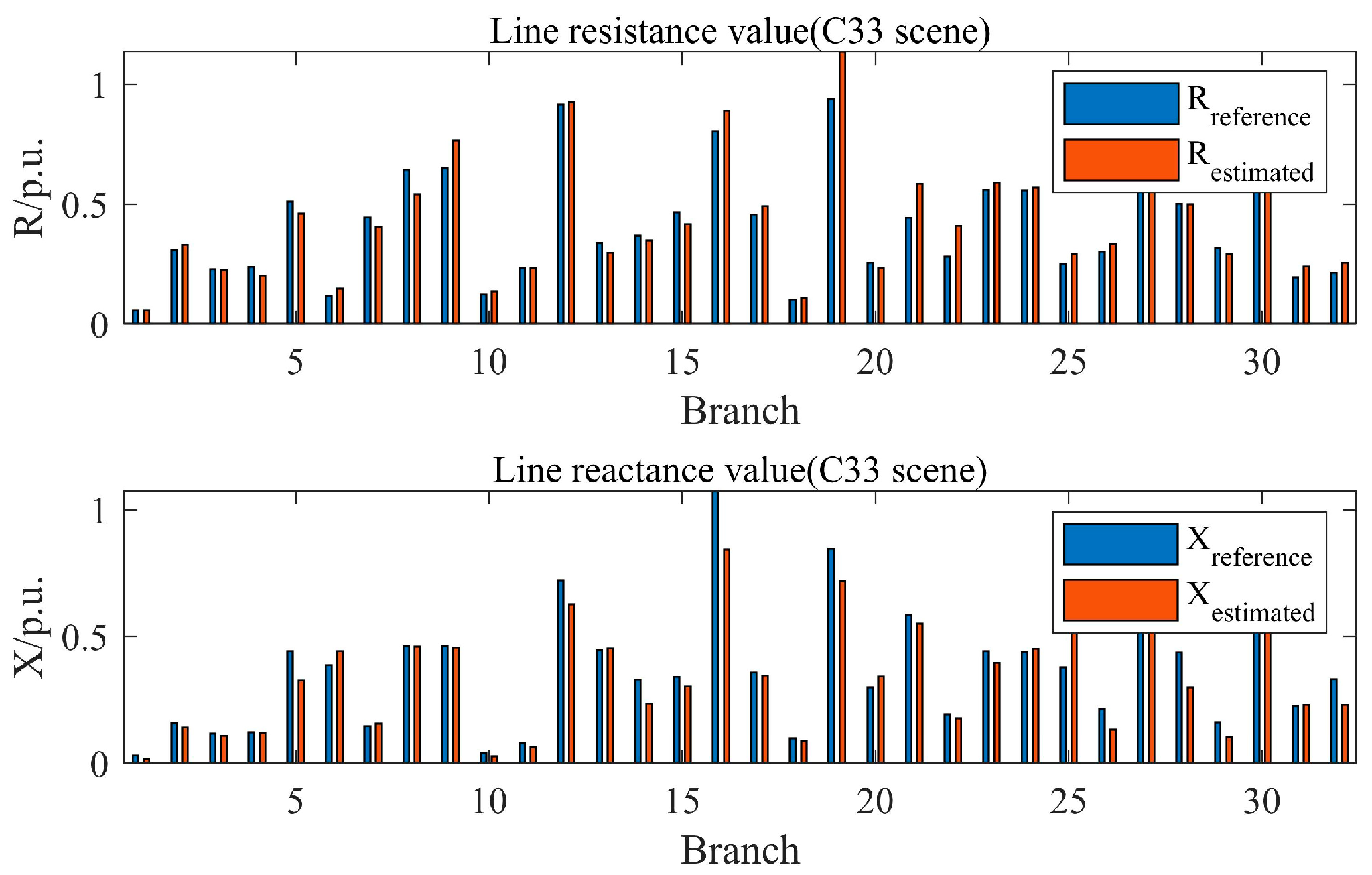
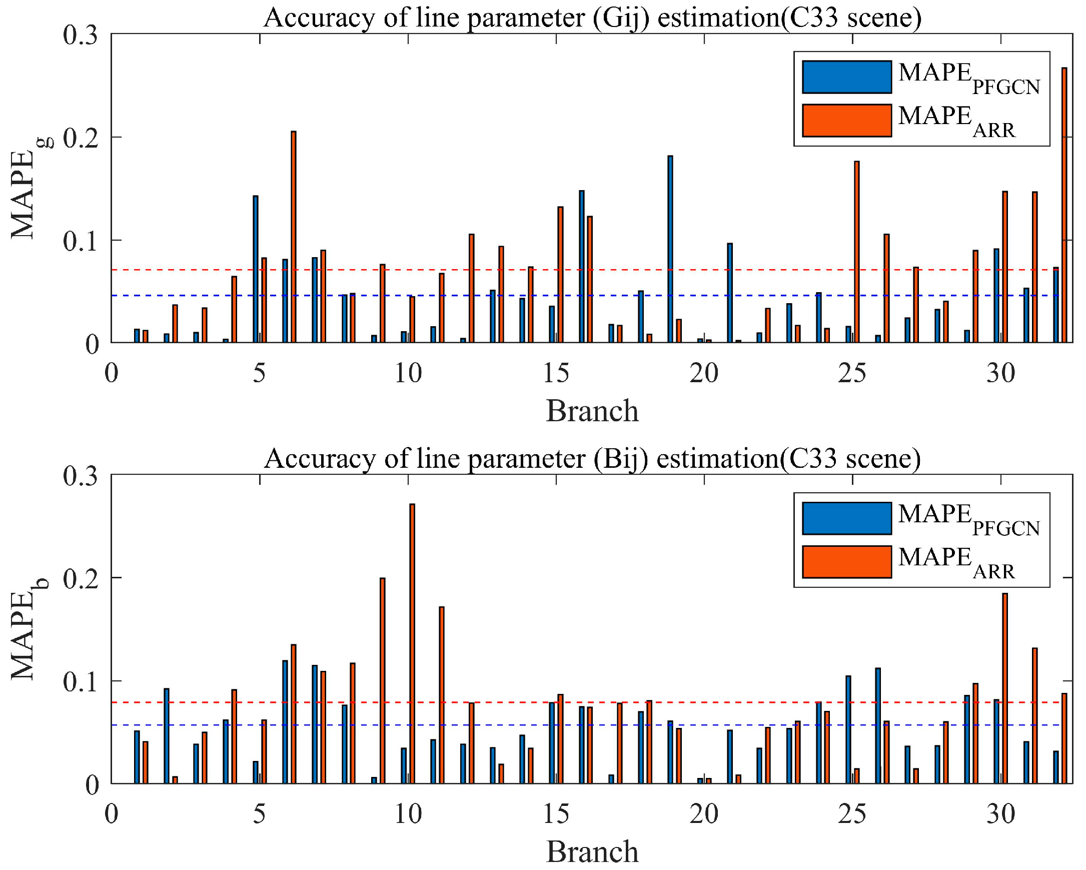
5.3.2. Parameter Estimation Results

In this subsection, we performed parameter identification experiments using the set of candidate topologies of scene C33 as topological inputs. The parameter estimation layer is set up with Adam optimizer, with learning rate $lr$ = 0.01 and iteration epoch = 30. Outer layer iteration threshold set $\xi$ = 0.05.

Table 2. C33 scene, candidate topologies and their final loss function values.

Group	Topology 1	Topology 2
$A_1$	1	0.9963
$F$	1.03 × 10−5	4.47 × 10−3

shows the candidate topologies and their final loss function values $F$.

$A_1$$F$Figure 8 illustrates the variation in loss function values throughout the final training process for the C33 scenario, utilizing topology 1 and topology 2 as graph inputs to the parameter estimation model. Notably, the nodes exhibiting fluctuations indicate that the PFGCN’s convolutional kernel violated the properties of the conductor matrix during training. This issue was subsequently addressed by the property correction module, allowing the corrected kernel to be reintroduced into the training process. The parameter estimation model proposed in this paper is built on the original AC power flow equations. As a result, the correct topology and more accurate line parameters tend to yield lower loss function values during the training process. For instance, topology 1 achieves a smaller loss function value than topology 2, which contains erroneous line connections. This provides the foundation for the proposed topology screening process in the joint estimation method. The training process illustrated in Figure 8 and the final loss function results presented in Table 2 highlight the effectiveness of using loss function values to filter topologies.

In this study, the line parameter matrix and the convolution kernel in the parameter estimation layer are essentially the same, representing concepts from power system theory and neural network theory, respectively. Figure 9 presents the initial convolution kernel values and the final results for the C33 scenario. Figure 10 illustrates the theoretical and final estimated values of line impedance for the same scenario. The initial values, obtained via regression estimation while ignoring the phase angle, exhibit significant errors, with a MAPE of 104.8% for line conductance g and 102.3% for line susceptance b. After applying the iterative solution of the proposed parameter estimation model, the accuracy of the line parameter estimates improves significantly, with the MAPE reduced to 4.6% for g and 5.7% for b. These results demonstrate the validity of the proposed joint estimation model under ideal conditions (random error $\epsilon$ = 0) on the IEEE-33 system (scenario C33).

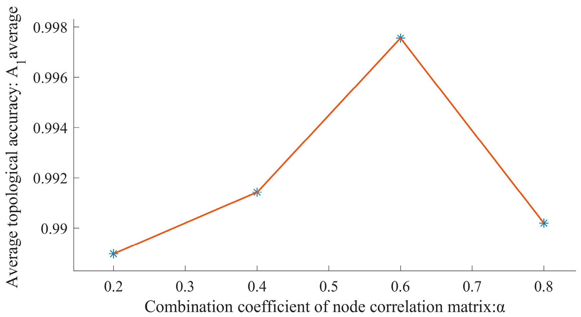
5.3.3. Impact Analysis of Parameter ${\alpha }_1$

In this subsection, we analyze the impact of the coefficients ${\alpha }_1$ based on scene C33. The coefficient ${\alpha }_1$ is a weighting factor regulating the amplitude dimension represented by the Euclidean distance and the percentage of the trend dimension of change represented by the DDTW distance. The experimental setup is as follows: C33: IEEE-33 system, 600 measurements, random error $\epsilon$ = 0. The data are grouped into 6 and set ${\alpha }_1$ = 0.2, 0.4, 0.6, 0.8.

Figure 11 shows the average accuracy results of the candidate topologies obtained for scene C33, ${\alpha }_1$ = 0.2, 0.4, 0.6, 0.8. As the value of ${\alpha }_1$ increases, the accuracy of topology identification initially improves, reaching its maximum at ${\alpha }_1$ = 0.6, after which it declines. This observation forms the basis for the ${\alpha }_1$ parameter setting in this paper. The experimental results demonstrate that the combined Euclidean and DDTW distance methods outperform single-dimension evaluation methods.

In conclusion, the experiments conducted in scenario C33 confirm the effectiveness of the proposed joint estimation method for topology and parameter identification. Additionally, the experiments validate that the correlation assessment method presented in this paper, which integrates both the magnitude and trend of changes, is superior to approaches that consider only a single dimension.

5.4. Improved IEEE-69 System Test Results

5.4.1. Analysis of Topology Identification Results

In order to validate the extensibility of the method proposed in this paper, we conducted tests based on the improved IEEE-69 system. In this subsection, experiments with the topology recognition algorithm are conducted in the IC69 scene. The data grouping is 6. Set ${\alpha }_1$ = 0.6.

Table 3. IC69 scene, ${\alpha }_1$ = 0.6, candidate topology results.

Group	1	2	3	4	5	6
$A_1$	1	1	0.9992	1	0.9983	0.9992

presents the candidate topology identification results for the IC69 scene. The candidate topology set includes the correct topologies, confirming the effectiveness of the proposed topology identification method in improving the performance of the IEEE-69 system.

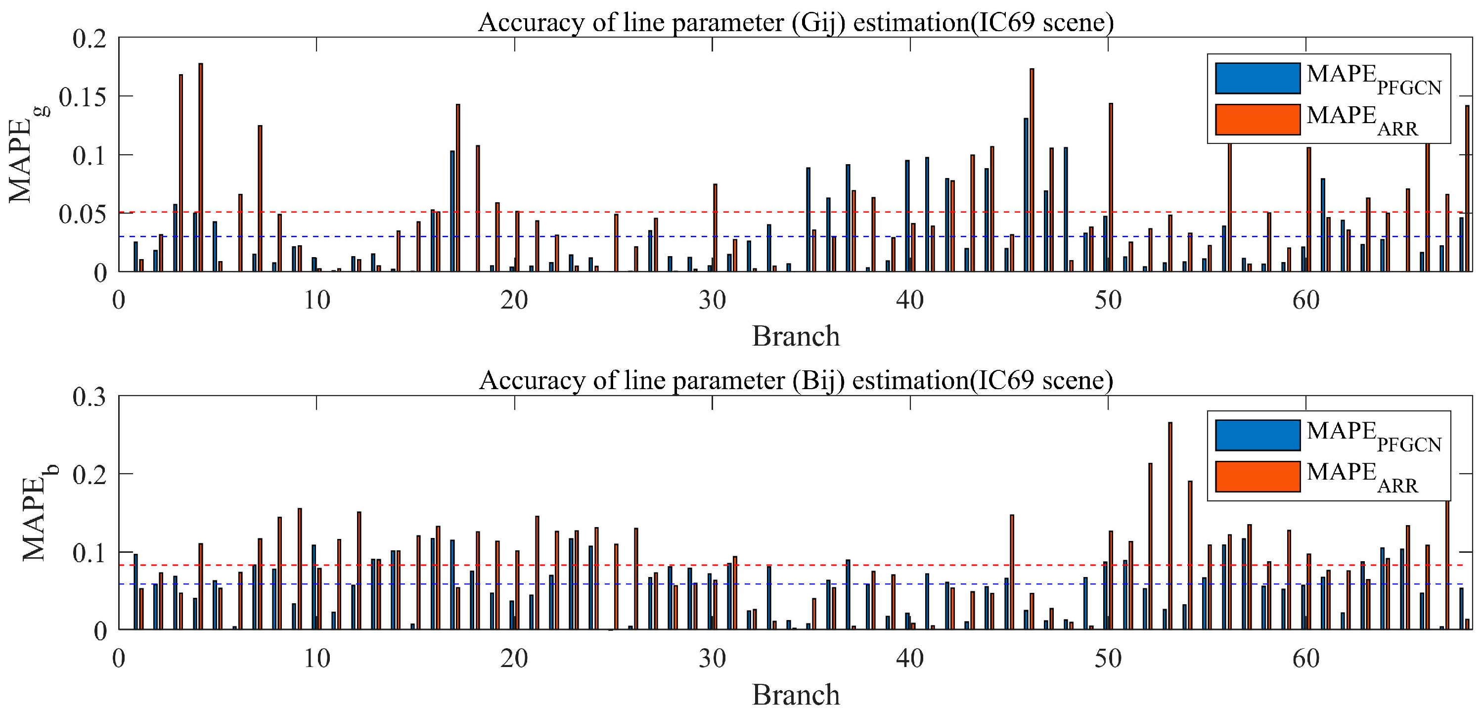
5.4.2. Analysis of Parameter Estimation Results

In this subsection, we performed parameter identification experiments in the IC69 scene. The parameter estimation layer is set up with Adam optimizer, with learning rate $lr$ = 0.01 and iteration epoch = 30. Outer layer iteration threshold set $\xi$ = 0.05.

Figure 12 shows the initial values obtained from regression estimation and the final estimation results of the line parameters for the IC69 scene. Figure 13 illustrates the same scenario’s theoretical and final estimated line impedance values. Similar to the results in scene C33, the initial values of the line parameters from regression estimation exhibit significant errors, with an average MAPE of 102.9% for g and 112.5% for b. After applying the parameter estimation model, the accuracy of the line parameter estimates improves significantly, reducing the average MAPE to 3.0% for g and 5.9% for b.

In summary, experiments conducted on the improved IEEE-69 system demonstrate the scalability of the method proposed in this paper, demonstrating the topological adaptation of the PF-GCN parameter identification model.

5.5. Algorithm Comparison

Algorithm comparison experiments are conducted in this section to evaluate the proposed method’s performance further. In Section 5.3.3, it was demonstrated that the proposed topology identification method, which integrates data amplitude and trend, outperforms methods based on a single perspective. This section focuses on comparing different parameter identification methods. A recent study [17] employed the cross-iterative estimation method and applied adaptive ridge regression (ARR) for parameter estimation, demonstrating superiority over traditional linear regression. Thus, the ARR method from [17] is selected as a control group for the proposed method. In both the C33 and IC69 scenarios, the correct topology is fixed as input for parameter estimation. PFGCN method: the parameter estimation layer is set up with Adam optimizer, with learning rate $lr$ = 0.01 and iteration epoch = 30. Outer layer iteration threshold set $\xi$ = 0.05. ARR method: set the regularization factor $\kappa$ = 0.003, adaptive coefficients $\delta$ = 5 × 10⁻⁵, $\gamma$ = 2, and set the iteration threshold $\xi$ = 0.05. Figure 14 and Figure 15 illustrate the parameter estimation performance of the PFGCN method and the adaptive ridge regression (ARR) method for the C33 and IC69 scenarios, respectively.

Table 4. Performance comparison of PFGCN algorithm and ARR algorithm for C33 and IC69 scenarios.

Scene		CV-GCN	ARR
C33	$MAP{E}_g$	0.046	0.071
	$MAP{E}_b$	0.057	0.079
	$IA{E}_g$	2.605	5.053
	$IA{E}_b$	3.748	5.223
	$MA{E}_g$	0.081	0.158
	$MA{E}_b$	0.117	0.163
	${R^2}_g$	0.999	0.998
	${R^2}_b$	0.996	0.992
IC69	$MAP{E}_g$	0.030	0.051
	$MAP{E}_b$	0.059	0.083
	$IA{E}_g$	15.892	37.296
	$IA{E}_b$	21.616	30.204
	$MA{E}_g$	0.234	0.548
	$MA{E}_b$	0.318	0.444
	${R^2}_g$	0.999	0.991
	${R^2}_b$	0.997	0.993

compares multiple evaluation metrics, including MAPE, IAE, MAE, and R², between the PFGCN method and the ARR method.

In the same scenario, the PFGCN method achieves better results than the ARR algorithm in all the metrics, and the line parameter estimation accuracy of the PFGCN method is higher. Specifically, in the C33 scenario, the PF-GCN method achieves MAPE values of 4.6% for g and 5.7% for b, significantly lower than the ARR algorithm’s 7.1% for g and 7.9% for b. The PF-GCN method also yields IAE values of 2.605 for g and 3.748 for b, much lower than the ARR algorithm’s 5.053 for g and 5.223 for b. Additionally, the PF-GCN method achieves MAE values of 0.081 for g and 0.117 for b, compared to the ARR algorithm’s 0.158 for g and 0.163 for b. Furthermore, the PF-GCN method attains R² values of 0.999 for g and 0.996 for b, higher than the ARR algorithm’s 0.998 for g and 0.992 for b.

Similarly, in the IC69 scenario, the PF-GCN method achieves MAPE values of 3.0% for g and 5.9% for b, outperforming the ARR method’s 5.1% for g and 8.3% for b. The PF-GCN method also yields IAE values of 15.892 for g and 21.616 for b, significantly lower than the ARR algorithm’s 37.296 for g and 30.204 for b. Additionally, it achieves MAE values of 0.234 for g and 0.318 for b, compared to the ARR algorithm’s 0.548 for g and 0.444 for b. Moreover, the PF-GCN method attains R² values of 0.999 for g and 0.997 for b, higher than the ARR algorithm’s 0.991 for g and 0.992 for b.

Based on the experiments conducted in the C33 and IC69 scenarios and multiple evaluation metrics, the proposed PFGCN method demonstrates superior line parameter identification accuracy compared to the ARR algorithm.

5.6. Error Sensitivity Analysis

Since acquiring ideal measurement data ($\epsilon$ = 0) in real distribution networks is complex, this section conducts error sensitivity experiments to analyze the robustness of the joint estimation method proposed in this paper. Considering the accuracy of the actual distribution network data devices, we set two random error levels $\epsilon$ = 0.1%, 0.2% for both the IEEE-33 system and the improved IEEE-69 system measurements. A total of 600 sets of voltage amplitude and power measurement data are simulated by MATPOWER for each scene. We set the scenes as follows:

• C33_0.1: IEEE-33 system, 600 measurements, random error $\epsilon$ = 0.1%;
• C33_0.2: IEEE-33 system, 600 measurements, random error $\epsilon$ = 0.2%;
• IC69_0.1: Improved IEEE-69 system, 600 measurements, random error $\epsilon$ = 0.1%.
• IC69_0.2: Improved IEEE-69 system, 600 measurements, random error $\epsilon$ = 0.2%.

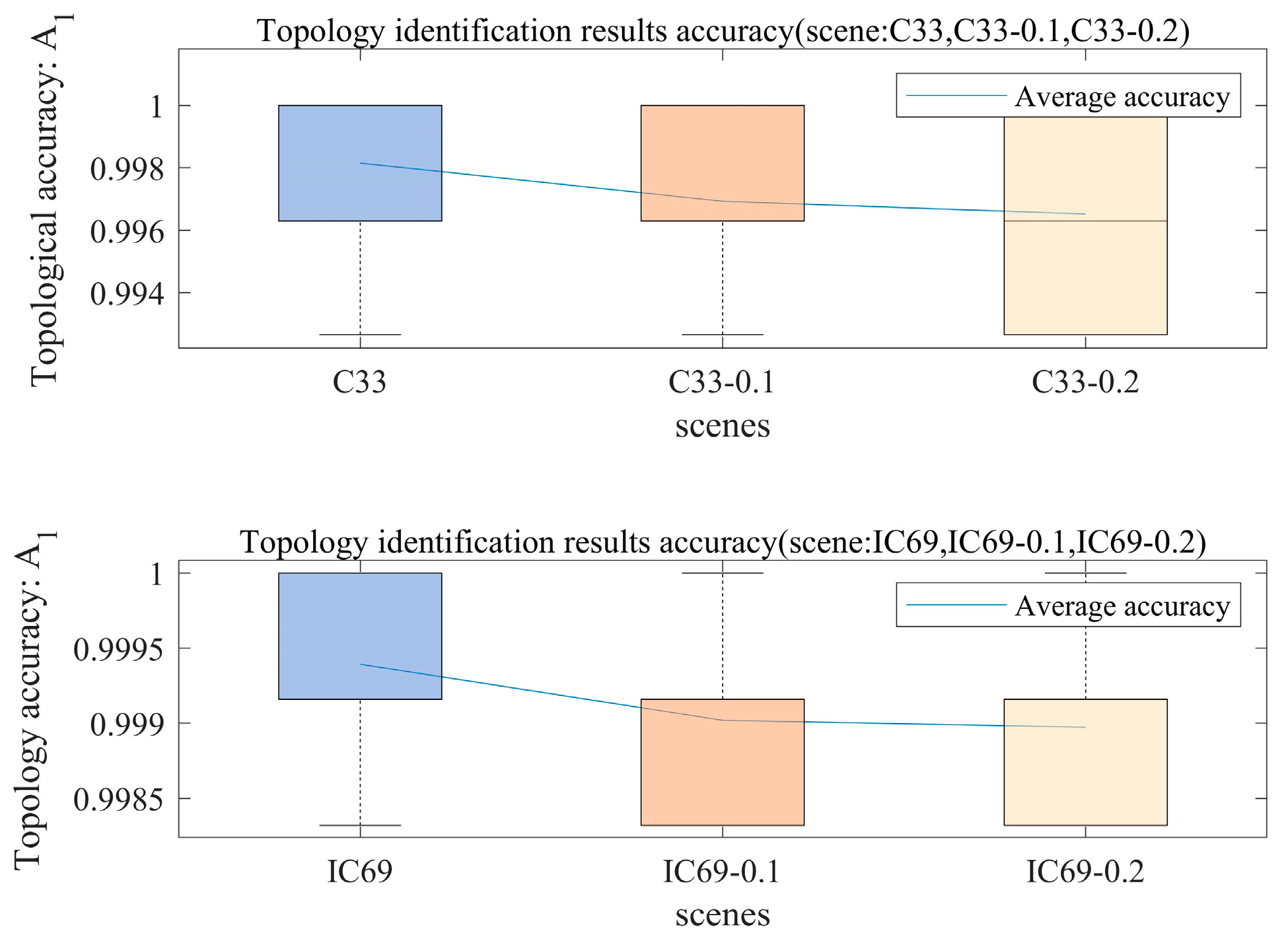
5.6.1. Error Sensitivity Analysis of Topology Identification Methods

This subsection analyzes the effect of the error on the candidate topology results for the IEEE-33 system and the improved IEEE-69 system. The data grouping is set to be 6, and the combination coefficient ${\alpha }_1$ of the matrix $K$ is set to be 0.6 (${\alpha }_1$ = 0.6). Figure 16 illustrates the candidate topology accuracy results for the IEEE-33 system and the improved IEEE-69 system obtained from multiple repetitive experiments.

As the error level increases, the topology identification accuracy of both the IEEE-33 and the improved IEEE-69 systems shows a gradual decline. At the same error level, the proportion of correct topologies among the candidate topologies for the IEEE-33 system is slightly higher than that for the improved IEEE-69 system. However, due to the grouping strategy employed, the set of candidate topologies for both systems still contains correct topologies at error levels of 0.1% and 0.2%. This demonstrates that the topology identification method proposed in this paper remains effective under these conditions.

5.6.2. Error Sensitivity Analysis of Parameter Estimation Methods

This subsection examines the impact of errors on line parameter estimation in both the IEEE-33 and the improved IEEE-69 systems. The candidate topologies obtained from different scenarios in the previous section are used as graph inputs for the corresponding line parameter estimation models. The parameter estimation layer is set up with Adam optimizer, with learning rate $lr$ = 0.01 and iteration epoch = 30. Outer layer iteration threshold set $\xi$ = 0.05.

Table 5. Comparison of line parameter identification accuracy for different error levels (scene: C33, C33_0.1, C33_0.2, IC69, IC69_0.1, IC69_0.2).

Scene	C33	C33_0.1	C33_0.2	IC69	IC69_0.1	IC69_0.2
$map{e}_g$	0.046	0.061	0.059	0.030	0.063	0.076
$map{e}_b$	0.057	0.075	0.088	0.059	0.084	0.091

presents the parameter estimation accuracy results for the IEEE-33 system (scenarios: C33, C33_0.1, C33_0.2) and the improved IEEE-69 system (scenarios: IC69, IC69_0.1, IC69_0.2) at different error levels. The results indicate that the line parameter estimation accuracy for both systems decreases as the error level increases. Specifically, for the IEEE-33 system, the MAPE of g increases from 4.6% to 5.9%, and the MAPE of b rises from 5.7% to 8.8%. For the improved IEEE-69 system, the MAPE of g grows from 3.0% to 7.6%, while the MAPE of b increases from 5.9% to 9.1%. Despite the error growth, the MAPE of both g and b remains below 10% across all six scenes.

$map{e}_g$$map{e}_b$In summary, the experiments confirm that the joint identification method proposed in this paper is robust. It maintains high identification accuracy and robustness even in the presence of random errors in the measurement data.

6. Conclusions

This paper proposes a joint topology parameter identification method based on PFGCN to address the challenges of topology identification and parameter estimation in distribution networks. In the topology identification stage, a node correlation matrix is defined using both Euclidean and DDTW distances. A minimum distance iteration algorithm is introduced to construct the candidate topology set. This method assesses node correlation in magnitude and trend, offering strong robustness and improved identification accuracy.

In the parameter estimation stage, the AC power flow equations are reformulated using complex-valued graph convolution, and a new trend graph convolutional network is constructed, with the candidate topology serving as the graph input. This network enhances line parameter identification accuracy while providing interpretability and adaptability to topology variations. Additionally, this method avoids using voltage phase angle measurements, circumventing the high costs associated with PMU deployment and improving practical applicability.

Experiments conducted on the IEEE-33 and improved IEEE-69 systems demonstrate the proposed method’s superior accuracy and confirm its robustness, scalability, and adaptability.

In this paper, power flow graph convolutional networks are developed based on traditional graph convolutional networks. Emphasis is placed on the network’s transformation and its performance evaluation. Our future research will focus on exploring other deeper features of the network, identifying the limitations in its application, and defining the boundaries of its function.

References

1. Wang, X.; Zhao, Y.; Zhou, Y. A Data-Driven Topology and Parameter Joint Estimation Method in Non-PMU Distribution Networks. IEEE Trans. Power Syst. 2024, 39, 1681–1692. [Google Scholar] [CrossRef]
2. Park, S.; Deka, D.; Chertkov, M. Exact Topology and Parameter Estimation in Distribution Grids with Minimal Observability. In Proceedings of the 2018 Power Systems Computation Conference (PSCC), Dublin, Ireland, 11–15 June 2018. [Google Scholar]
3. Dehghanpour, K.; Wang, Z.; Wang, J.; Yuan, Y.; Bu, F. A Survey on State Estimation Techniques and Challenges in Smart Distribution Systems. IEEE Trans. Smart Grid 2019, 10, 2312–2322. [Google Scholar] [CrossRef]
4. Dong, X.; Kang, C.; Sun, H.; Zhang, N. Analysis of Power Transfer Limit Considering Thermal Balance of Overhead Conductor. IET Gener. Transm. Distrib. 2015, 9, 2007–2013. [Google Scholar] [CrossRef]
5. Cavraro, G.; Arghandeh, R. Power Distribution Network Topology Detection with Time-Series Signature Verification Method. IEEE Trans. Power Syst. 2018, 33, 3500–3509. [Google Scholar] [CrossRef]
6. Pappu, S.J.; Bhatt, N.; Pasumarthy, R.; Rajeswaran, A. Identifying Topology of Low Voltage Distribution Networks Based on Smart Meter Data. IEEE Trans. Smart Grid 2018, 9, 5113–5122. [Google Scholar] [CrossRef]
7. Deka, D.; Backhaus, S.; Chertkov, M. Structure Learning in Power Distribution Networks. IEEE Trans. Control Netw. Syst. 2017, 5, 1061–1074. [Google Scholar] [CrossRef]
8. Zhao, J.; Li, L.; Xu, Z.; Wang, X. Full-Scale Distribution System Topology Identification Using Markov Random Field. IEEE Trans. Smart Grid 2020, 11, 4714–4726. [Google Scholar] [CrossRef]
9. Ma, L.; Wang, L. Topology Identification of Distribution Networks Using a Split-EM Based Data-Driven Approach. IEEE Trans. Power Syst. 2021, 37, 2019–2031. [Google Scholar] [CrossRef]
10. Pegoraro, P.A.; Brady, K.; Muscas, C. Line Impedance Estimation Based on Synchrophasor Measurements for Power Distribution Systems. IEEE Trans. Instrum. Meas. 2018, 68, 1002–1013. [Google Scholar] [CrossRef]
11. Dutta, R.; Patel, V.S.; Chakrabarti, S.; Sharma, A. Parameter Estimation of Distribution Lines Using SCADA Measurements. IEEE Trans. Instrum. Meas. 2020, 70, 1–11. [Google Scholar] [CrossRef]
12. Lave, M.; Reno, M.J.; Peppanen, J. Distribution System Parameter and Topology Estimation Applied to Resolve Low-Voltage Circuits on Three Real Distribution Feeders. IEEE Trans. Sustain. Energy 2019, 10, 1585–1592. [Google Scholar] [CrossRef]
13. Srinivas, V.L.; Wu, J. Topology and Parameter Identification of Distribution Network Using Smart Meter and μPMU Measurements. IEEE Trans. Instrum. Meas. 2022, 71, 1–14. [Google Scholar] [CrossRef]
14. Zhang, J.; Wang, Y.; Weng, Y.; Zhang, N. Topology Identification and Line Parameter Estimation for Non-PMU Distribution Network: A Numerical Method. IEEE Trans. Smart Grid 2020, 11, 4440–4453. [Google Scholar] [CrossRef]
15. Wang, C.; Lou, Z.; Li, M.; Zhu, C.; Jing, D. Identification of Distribution Network Topology and Line Parameter Based on Smart Meter Measurements. Energies 2024, 17, 830. [Google Scholar] [CrossRef]
16. Ni, J.; Tang, Z.; Liu, J.; Zeng, P.; Baldorj, C. A Topology Identification Method Based on One-Dimensional Convolutional Neural Network for Distribution Network. Energy Rep. 2023, 9, 355–362. [Google Scholar] [CrossRef]
17. Yang, X.; Jiang, J.; Liu, F.; Tang, J. Hybrid Data and Model-driven Joint Identification of Distribution-network Topology and Parameters. IET Gener. Trans. Distrib. 2022, 16, 4846–4866. [Google Scholar] [CrossRef]
18. Sun, J.; Xia, M.; Chen, Q. A Classification Identification Method Based on Phasor Measurement for Distribution Line Parameter Identification Under Insufficient Measurements Conditions. IEEE Access 2019, 7, 158732–158743. [Google Scholar] [CrossRef]
19. Wang, Z.; Xia, M.; Lu, M.; Pan, L.; Liu, J. Parameter Identification in Power Transmission Systems Based on Graph Convolution Network. IEEE Trans. Power Deliv. 2021, 37, 3155–3163. [Google Scholar] [CrossRef]
20. Li, H.; Blasch, E. Distribution Grid Topology and Parameter Estimation Using Deep-Shallow Neural Network with Physical Consistency. IEEE Trans. Smart Grid 2023, 15, 655–666. [Google Scholar] [CrossRef]
21. Wang, W.; Yu, N. Estimate Three-Phase Distribution Line Parameters with Physics-Informed Graphical Learning Method. IEEE Trans. Power Syst. 2022, 37, 3577–3591. [Google Scholar] [CrossRef]
22. Liu, S.; Wu, C.; Zhu, H. Topology-Aware Graph Neural Networks for Learning Feasible and Adaptive AC-OPF Solutions. IEEE Trans. Power Syst. 2023, 38, 1–11. [Google Scholar] [CrossRef]
23. Sinaga, K.P.; Hussain, I.; Yang, M.-S. Entropy K-Means Clustering with Feature Reduction Under Unknown Number of Clusters. IEEE Access 2021, 9, 67736–67751. [Google Scholar] [CrossRef]
24. Luczak, M. Hierarchical Clustering of Time Series Data with Parametric Derivative Dynamic Time Warping. Expert Syst. Appl. 2016, 62, 116–130. [Google Scholar] [CrossRef]
25. Liang, H.; Ma, J. Develop Load Shape Dictionary Through Efficient Clustering Based on Elastic Dissimilarity Measure. IEEE Trans. Smart Grid 2021, 12, 442–452. [Google Scholar] [CrossRef]
26. Niepert, M.; Ahmed, M.; Kutzkov, K. Learning Convolutional Neural Networks for Graphs. arXiv 2016, arXiv:1605.05273. [Google Scholar] [CrossRef]
27. Trabelsi, C.; Bilaniuk, O.; Zhang, Y.; Serdyuk, D.; Subramanian, S.; Santos, J.F.; Mehri, S.; Rostamzadeh, N.; Bengio, Y.; Pal, C.J. Deep Complex Networks. arXiv 2017, arXiv:1705.09792. [Google Scholar]
Figure 1. A framework for joint estimation of topology and line parameters.
Energies 17 05272 g001
Figure 2. The structure of a single line.
Energies 17 05272 g002
Figure 3. The framework of the line parameter estimation model.
Energies 17 05272 g003
Figure 4. Infrastructure for the power flow graph convolutional network.
Energies 17 05272 g004
Figure 5. Topology of the 33-node system.
Energies 17 05272 g005
Figure 6. Topology for the improved 69-node system.
Energies 17 05272 g006
Figure 7. C33 scene, α 1 = 0.6, 6-group node correlation matrix K 1 K 6 results.
Energies 17 05272 g007
Figure 8. The values of the loss function F for the training process in the C33 scenario for topology 1 and topology 2.
Energies 17 05272 g008
Figure 9. C33 scene, the initial value of the convolution kernel obtained from regression estimation and the final result of the convolution kernel after training.
Energies 17 05272 g009
Figure 10. Comparison between reference values and estimated results for C33 scenario line parameters.
Energies 17 05272 g010
Figure 11. The average of the accuracy A 1 of the candidate topologies, C33 scene, α 1 = 0.2, 0.4, 0.6, 0.8.
Energies 17 05272 g011
Figure 12. IC69 scene, the initial value of the convolution kernel obtained from regression estimation and the final result of the convolution kernel after training.
Energies 17 05272 g012
Figure 13. Comparison between reference values and estimated results for IC69 scene line parameters.
Energies 17 05272 g013
Figure 14. Line parameter estimation accuracy of PFGCN and ARR Models for Scenario C33.
Energies 17 05272 g014
Figure 15. Line parameter estimation accuracy of PFGCN and ARR Models for Scenario IC69.
Energies 17 05272 g015
Figure 16. Candidate topology accuracy results for IEEE-33 system (C33, C33_0.1, C33_0.2) and improved IEEE-69 system (IC69, IC69_0.1, IC69_0.2) with different error levels ( ε = 0.1%, 0.2%).
Energies 17 05272 g016