Fault Diagnosis Method for Hydropower Units Based on Dynamic Mode Decomposition and the Hiking Optimization Algorithm–Extreme Learning Machine

Abstract

The diagnosis of vibration faults in hydropower units is essential for ensuring the safe and stable operation of these systems. This paper proposes a fault diagnosis method for hydropower units that combines Dynamic Mode Decomposition (DMD) with an optimized Extreme Learning Machine (ELM) utilizing the Hiking Optimization Algorithm (HOA). To address the issue of noise interference in the vibration signals of hydropower units, this study employs DMD technology alongside a thresholding technique for noise reduction, demonstrating its effectiveness through comparative trials. Furthermore, to facilitate a thorough analysis of the operational status of hydropower units, this paper extracts multidimensional features from denoised signals. To improve the efficiency of model training, Principal Component Analysis (PCA) is applied to streamline the data. Given that the weights and biases of the ELM are generated randomly, which may impact the model’s stability and generalization capabilities, the HOA is introduced for optimization. The HOA-ELM model achieved a classification accuracy of 95.83%. A comparative analysis with alternative models substantiates the superior performance of the HOA-ELM model in the fault diagnosis of hydropower units.

1. Introduction

Hydropower units serve as the fundamental components of hydroelectric power stations. Their extended operation in complex stress environments, characterized by hydraulic and mechanical loads, may result in internal fatigue, aging, component loosening, and insulation degradation. Consequently, it is imperative to conduct fault diagnosis on these units [1].

Vibration is a fundamental indicator of the operational condition of a power unit, encapsulating the unit’s status characteristics and providing a significant amount of fault-related information. The analysis of vibration signals from hydropower units is a critical aspect of research focused on condition monitoring and fault diagnosis [2,3]. In addressing the challenges posed by the nonlinearity, non-stationarity, and elevated noise levels inherent in vibration signals, various time–frequency analysis techniques are frequently utilized. These techniques include the Short-Time Fourier Transform (STFT) [4], Wavelet Transform (WT) [5], and Empirical Mode Decomposition (EMD) [6]. WT addresses the limitations of STFT regarding fixed resolution, enabling a more precise analysis of the true frequency components of the signal [7,8]. However, the selection of the basis function for WT and the determination of the number of decomposition levels exhibit a lack of adaptivity. In contrast, EMD, which relies on the distribution of a signal’s extreme points, obviates the necessity for basis function selection [9], but it is prone to issues related to mode mixing. In 2010, Peter Schmid et al. [10] introduced DMD, a method that efficiently and intuitively reveals the fundamental dynamics of complex systems, resulting in its extensive application in multivariate time series analysis and fault detection. Chen Changzhe et al. [11] utilized high-order DMD for the prediction of time series related to ship maneuvering under wave conditions. To address the challenges posed by incomplete data from single-sensor measurements and the excessive data generated by the straightforward application of multi-sensor data, Li Junqing et al. [12] introduced the DMD signal decomposition approach. This method decomposes multi-sensor signals into multiple modes and reconstructs the original signal using the mode with the maximum energy value.

Currently, intelligent algorithms that utilize machine learning and deep learning technologies are widely employed in the field of fault diagnosis for hydropower units. Yang Tong et al. [13] employed a Hybrid Grey Wolf Optimizer (HGWO) to perform global optimization of kernel function coefficients and penalty parameters in Support Vector Machines (SVMs), thereby achieving optimal classification performance for the fault diagnosis of hydropower units. Hu Xiao et al. [14] proposed a fault diagnosis method that combines Variational Mode Decomposition (VMD) with Convolutional Neural Networks (CNNs). Nevertheless, the elevated complexity of the models employed in these methods poses significant challenges in fulfilling the efficiency requirements of practical applications. In contrast, the ELM model, characterized by its straightforward architecture and high computational efficiency, is well-suited for rapid and effective classification and recognition tasks. He Kuidong et al. [15] proposed a signal feature extraction method based on Ensemble Empirical Mode Decomposition (EEMD) and Multi-Scale Entropy (MSE) and then utilized the ELM to implement vibration fault diagnosis for hydropower units.

Therefore, this paper employs DMD technology to mitigate noise in the vibration signals of hydropower units. The vibration signals collected from these units often demonstrate pronounced nonlinear and non-stationary characteristics [16]. Consequently, the mere extraction of time-domain and frequency-domain features is inadequate for comprehensively capturing the relationship between the signals and the associated faults. Entropy features, which are indicators for quantifying the uncertainty in information [17], along with time–frequency features that encapsulate extensive information regarding the operational conditions of the equipment [18], are extracted. This extraction includes energy entropy, root mean square, and singular value features of each modal component, facilitating a comprehensive analysis of the unit’s operating conditions. PCA is then used for dimensionality reduction, which enhances model efficiency and addresses the problem of feature redundancy [19]. Finally, leveraging the straightforward architecture and rapid computational efficiency of the ELM, a model based on the ELM is developed to facilitate the classification of faults in hydropower units. The random assignment of weights and biases in the ELM can significantly impact the model’s stability and generalization capabilities. To mitigate this issue, the present study employs the HOA to optimize the initial parameters of the ELM, thereby enhancing the accuracy of fault diagnosis.

2. Fundamental Theory

2.1. Dynamic Mode Decomposition

Dynamic Mode Decomposition (DMD) performs the function of noise reduction through the decomposition and reconstruction of the original signal. By sampling the time series signal at uniform intervals, one can form a multivariate time series. If we assume that the combined multivariate time series consists of N individual time series signals, each with a length of M, then for any given moment t, the expression for DMD can be articulated as follows [20]:

$$x_t=A{x}_{t-1}$$

(1)

where A represents the Koopman matrix in DMD, with dimensions of N × N.

The specific algorithm is as follows:

(1)

Construct the matrix.

$$X=\left[\begin{array}{cccc}{x}_1& x_2& \cdots & x_{M-1}\end{array}\right]$$

(2)

$$Y=\left[\begin{array}{cccc}{x}_2& x_3& \cdots & x_M\end{array} \right]$$

(3)

(2)

Perform Singular Value Decomposition (SVD) on matrix X, that is,

$$X=U\Sigma V^{*}$$

(4)

where $U\in C^{N\times N}\mathrm{a}\mathrm{n}\mathrm{d}V\in C^{\left(\mathrm{M}-1\right)\times \left(\mathrm{M}-1\right)}$ are orthogonal matrices; $\Sigma \in C^{N\times \left(\mathrm{M}-1\right)}$ is a diagonal matrix.

(3)

Construct the matrix$\tilde{A}$, that is,

$$A={YV\Sigma }^{-1}{U}^{*}\Rightarrow \tilde{A}=U^{*}AU=U^{*}{YV\Sigma }^{-1}$$

(5)

where $A\in C^{N\times N},\tilde{A}\in C^{K\times K},K\ll N.$

(4)

Perform an eigenvalue decomposition on $\tilde{A}$, that is,

$$\tilde{A}W=W\Lambda$$

(6)

(5)

Reconstruct the eigenvalue decomposition of $A$, where the eigenvalues of $A$ are given by $\Lambda$, and the eigenvector matrix $\Psi$ of $A$ is given by W and U, that is,

$$\Psi =UW$$

(7)

(6)

Determine growth rate Re(${\omega }_k$) and frequency $f_k$ of the dynamic modes by taking the logarithm of the eigenvalues, that is,

$${\omega }_k={\displaystyle \frac{ln\left({\lambda }_k\right)}{\mathsf{\Delta }t}}=Re\left({\omega }_k\right)+Im\left({\omega }_k\right)$$

(8)

$${ f}_k={\displaystyle \frac{Im\left({\omega }_k\right)}{2\pi }}$$

(9)

(7)

Project the vibration data at the initial time onto the original flow field to obtain the modal energy $E_k$, which is expressed as follows:

$${ E}_k={\displaystyle \frac{{\psi }_k{x}_1}{\parallel x_1\parallel }}$$

(10)

(8)

Express the initial amplitude vector b as follows:

$$b={\Psi }^{+}{x}_1$$

(11)

Solve for the approximate solution $X_{DMD}\left(t\right)$ at any future time.

$$X_{DMD}\left(t\right)=\sum _{k=1}^K{\psi }_{k}exp\left({\omega }_{k}t\right)b_k=\psi diag\left[exp\left({\omega }_{k}t\right)\right]b$$

(12)

2.2. Multidimensional Feature Extraction

The occurrence of mechanical equipment failure is characterized by significant deviations in vibrational signals compared with those produced under normal operational conditions. These deviations manifest in the form of alterations in probabilistic distributions and fluctuations in magnitude, which can be quantified through the extraction of a multidimensional feature set. To achieve a comprehensive representation of the machinery’s operational status, a holistic multidimensional feature matrix of the vibrational signals was developed. This matrix incorporates statistical analysis, Fourier transformation, and DMD time–frequency analytical techniques, resulting in a diverse spectrum of features. These features encompass time-domain characteristics, frequency-domain attributes, energy entropy metrics derived from DMD modalities, root mean square values, and singular value characteristics.

Time-domain features were employed to articulate the probabilistic and statistical characteristics of the original signal in the time domain. A total of eleven specific temporal features inherent to the original signal were extracted.

Frequency-domain features, obtained through spectral analysis following Fourier transformation, served as statistical indices within the frequency domain. A total of twelve features were extracted, encapsulating both the spectral convergence characteristics and the distribution of energy across the frequency spectrum of the original signal.

While time-domain and frequency-domain features effectively illustrate the distribution of vibration signals within their respective domains, the vibration signals obtained from hydropower units are often characterized by significant nonlinearity and non-stationarity. The exclusive extraction of time-domain and frequency-domain features does not adequately capture the relationship between the signals and their associated faults. Entropy features, which quantify the uncertainty in information, indicate that the entropy values of vibration signals tend to increase during equipment malfunctions. Consequently, energy entropy features are utilized as one of the criteria for distinguishing the various operational states of the machinery. Furthermore, time–frequency features contain a substantial amount of information that reflects the operational status of the machinery. For example, root mean square features indicate the variability in the signal, while singular value features represent the intrinsic characteristics of the signal matrix, demonstrating both rotational and scale invariance. In consideration of these factors, this research applied the DMD methodology to decompose the original vibration signals. This analysis facilitated the calculation of energy entropy, root mean square, and singular value features associated with the respective modal components. This approach generated a comprehensive array of multidimensional feature information derived from the original vibration signals. The procedural steps are detailed as follows:

(1)

Utilize the DMD method to decompose the original vibration signal into a series of Intrinsic Mode Function (IMF) components.

(2)

Calculate the energy entropy features [21], denoted as EF_i, for each IMF component.

$$E{S}_i={\int }_{-\infty }^{+\infty }\mid IM{F}_i\left(t\right){\mid }^{2}dt$$

(13)

$$E=\sum _{i=1}^{K}E{S}_i,i=\mathrm{1,2},\dots ,k$$

(14)

$$EF=-\sum _{i=1}^K\left({\displaystyle \frac{E{S}_i}{E}}\right)lg\left({\displaystyle \frac{E{S}_i}{E}}\right)$$

(15)

where $E{S}_i$ represents the energy value of each IMF component, and $E$ denotes the total energy of all IMF components.

(3)

Calculate the root mean square (RMS) features [22], denoted as $R{F}_i$, for each IMF component.

$$R{F}_i={\left[{\displaystyle \frac{1}{N}}{\int }_{-\infty }^{+\infty }\mid IM{F}_i\left(t\right){\mid }^{2}dt\right]}^{{\displaystyle \frac{1}{2}}}i=\mathrm{1,2},\dots ,k$$

(16)

(4)

Calculate the singular value features [23], denoted as $SV{F}_i$, for the corresponding IMF components of the original signal.

$$\left\{\begin{array}{l}A=U\Lambda V^T\\ SV{F}_i=[{\lambda }_1,{\lambda }_2,\dots ,{\lambda }_i]i=\mathrm{1,2},\dots ,k\end{array}\right.$$

(17)

where A denotes the matrix constructed from the IMF components, and U_m×m and V_n×n are the left and right singular matrices of A, respectively. Λ is an m × n diagonal matrix, and λ₁, λ₂, …, λ_k are the singular values of matrix A.

The time-domain and frequency-domain features extracted from the original signal were combined with energy entropy features, root mean square features, and singular value features to create a multidimensional feature vector, as illustrated in Figure 1. However, the straightforward amalgamation of these features inevitably leads to redundancy, which can adversely affect the accuracy and efficiency of fault diagnosis. Consequently, it was essential to conduct dimensionality reduction on the multidimensional features in order to identify the optimal features that exhibit minimal redundancy and maximal relevance to the fault types.

This paper employed PCA as a method for dimensionality reduction to address the problem of feature redundancy. By converting highly correlated feature variables into a set of mutually independent lower-dimensional variables, the complexity of the data was reduced, which in turn improved the training efficiency of the model. The procedure for PCA is as follows [24]:

(1)

The input data samples are converted into a standardized matrix.

(2)

The computation of the correlation coefficient matrix $G={\left(r_{ij}\right)}_{m\times m}$ is executed based on the standardized matrix, as delineated by Equation (18).

$$r_{ij}={\displaystyle \frac{{\displaystyle {\sum }_{s=1}^n}\left(x_{si}-{\overline{x}}_i\right)\left(x_{sj}-{\overline{x}}_j\right)}{\sqrt{{\displaystyle {\sum }_{s=1}^n}{\left(x_{si}-{\overline{x}}_i\right)}^2{\displaystyle {\sum }_{s=1}^n}{\left(x_{sj}-{\overline{x}}_j\right)}^2}}}$$

(18)

where the term $r_{ij}$ is designated as the correlation coefficient between the variables $x_i$ and $x_j$; n is the number of samples; m is the number of features; ${\overline{x}}_i$ is the arithmetic mean of the i-th variable; ${\overline{x}}_j$ is the arithmetic mean of the j-th variable; $x_{si}$ denotes the value of the i-th feature within the s-th sample; and $x_{sj}$ denotes the value of the j-th feature within the s-th sample.

(3)

The eigenvalue problem associated with the correlation matrix G is solved to ascertain the eigenvalues λ along with their respective eigenvectors.

(4)

Employing Equations (19) and (20), the contribution rate ${\kappa }_i$ and the cumulative contribution rate ${\eta }_i$ are computed [25].

$${ \kappa }_i={\displaystyle \frac{{\lambda }_i}{{\displaystyle {\sum }_{s=1}^m}{\lambda }_s}}\left(i=\mathrm{1,2},\cdots ,m\right)$$

(19)

$${\eta }_i={\displaystyle \frac{{\displaystyle {\sum }_{s=1}^i}{\lambda }_s}{\sum _{s=1}^m{\lambda }_s}}\left(\begin{array}{cccc}i=1,& 2,& \cdots ,& m\end{array}\right)$$

(20)

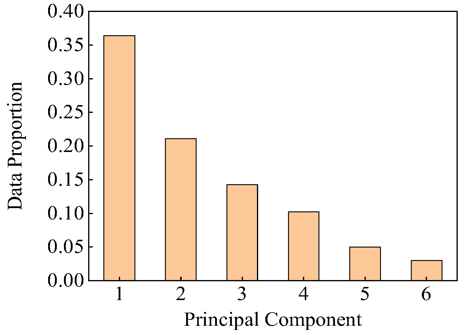
(5)

The number of principal components, denoted as k, is determined by the cumulative contribution rate of the explained variance. When the cumulative sum of the current k eigenvalues exceeds 90% of the total, the corresponding value of k is regarded as the number of principal components.

The distribution of the principal component data following dimensionality reduction is illustrated in Figure 2. In Figure 2, the cumulative proportion of the data represented by the first six principal components is 0.9007, indicating a cumulative contribution rate of 90.07%. Consequently, the six principal components illustrated in Figure 2 were selected as the input data for fault diagnosis.

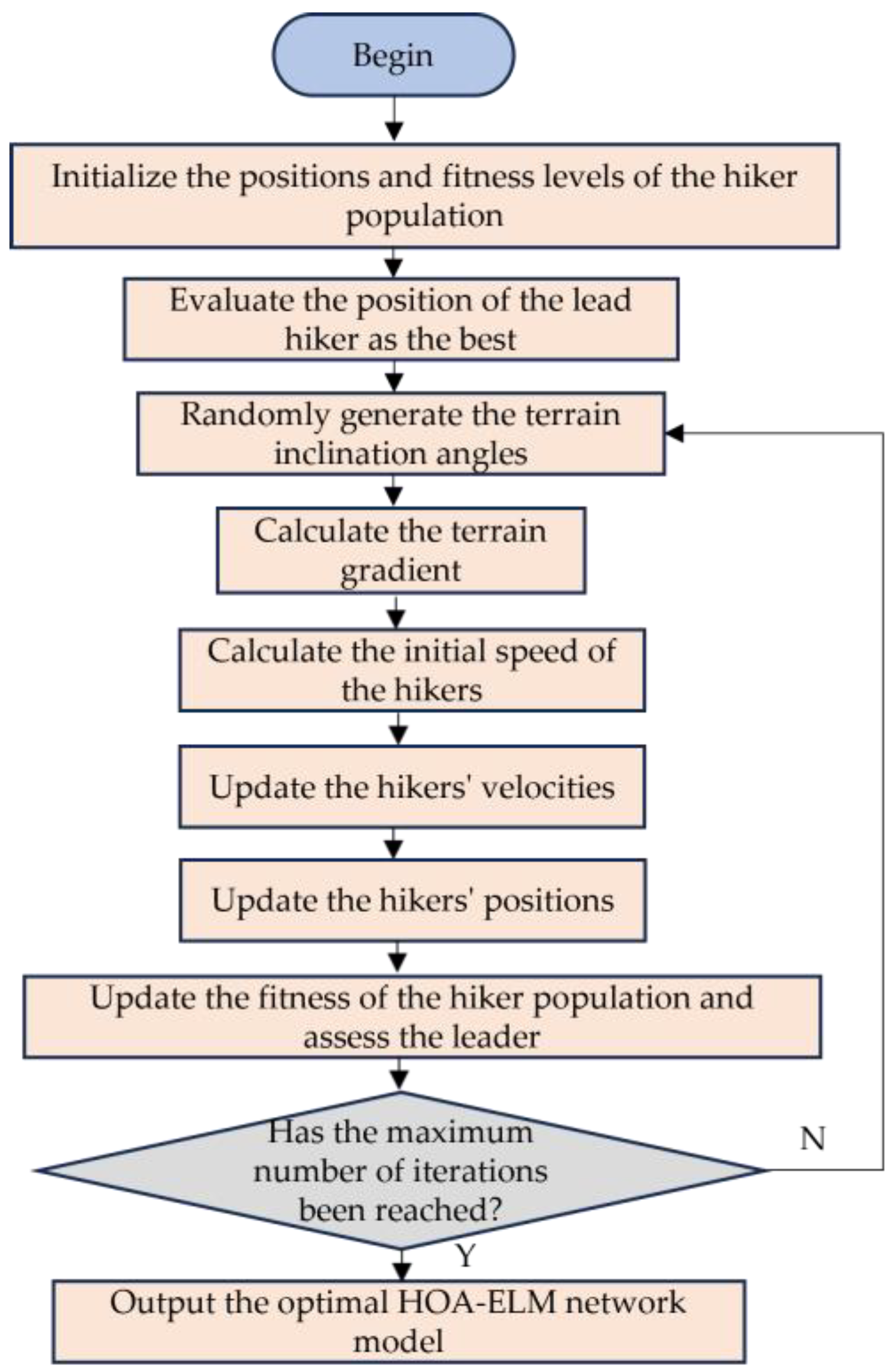
2.3. Hiking Optimization Algorithm

The Hiking Optimization Algorithm (HOA) is a meta-heuristic optimization technique inspired by the experience of hiking, as introduced by Oladejo et al. (2024) [26]. This algorithm addresses optimization problems by simulating the process of a hiker endeavoring to reach the summit of a mountain, hill, or rocky terrain.

The mathematical foundation of the HOA is based on Tobler’s Hiking Function (THF), which incorporates the steepness or gradient of the terrain or trail to assess the hiker’s speed.

$${\mathcal{W}}_{i,t}=6e^{-3.5\left|S_{i,t}+0.05\right|}$$

(21)

where ${\mathcal{W}}_{i,t}$ represents the speed of hiker i at iteration t and $S_{i,t}$ denotes the gradient of the terrain. Additionally, the calculation formula for $S_{i,t}$ is given by Equation (17)

$${ S}_{i,t}={\displaystyle \frac{dh}{dx}}=tan{\theta }_{i,t}$$

(22)

where $dh$ and $dx$ represent the altitude and horizontal distance traveled by the hiker, respectively. ${\theta }_{i,t}$ is the inclination angle of the terrain, with a value in the range [0°, 50°]. The HOA utilizes the social thinking of a group of hikers and the individual cognition of each hiker for updates. The current speed update formula for hikers in the HOA is

$${\mathcal{W}}_{i,t}={\mathcal{W}}_{i,t-1}+{\gamma }_{i,t}\left({\beta }_{best}-{\alpha }_{i,t}{\beta }_{i,t}\right)$$

(23)

where γ(i,t) is a random number within the range [0, 1]; ${\mathcal{W}}_{i,t}$ represents the speed of hiker i at iteration t; ${\beta }_{best}$ is the position of the leader; ${\beta }_{i,t}$ is the position of hiker i at iteration t; and ${\alpha }_{i,t}$ is the scanning factor SF of hiker i, where SF is within the range [1, 2], ensuring that hikers do not stray too far from the leader and allowing them to observe the leader’s direction and receive signals from the leader. By considering the hiker’s speed, the position update formula for hikers is

$${ \beta }_{i,t+1}={\beta }_{i,t}+W_{i,t}$$

(24)

The global exploration and local exploitation tendencies of the HOA are influenced by the scanning factor (SF). This factor notably impacts the distance between the leader and the other hikers, as demonstrated in Equation (23). Additionally, the gradient of the trail affects the speed of the hikers, as indicated in Equations (21) and (22), and it plays a critical role in both the global exploration and local exploitation components of the HOA.

As the SF range is expanded, the HOA tends to shift towards an exploitation phase. In contrast, a reduction in the SF range generally promotes an exploratory phase within the HOA. Additionally, a decrease in the range of the angle of inclination of the trail further directs the HOA towards the exploitation phase. Collectively, these factors play a significant role in influencing the behavior and performance of the HOA in addressing optimization problems. Algorithm 1 shows the implementation of the HOA.

Algorithm 1: HOA

Input: UB, LB, T, I, d $1: \mathcal{F}$$\leftarrow \mathrm{Preallocate} \mathrm{fitness} \mathrm{vector} {\mathbb{R}}^{I\times 1}$ $2: {\mathcal{F}}_{best}$$\leftarrow \mathrm{Preallocate} \mathrm{best} \mathrm{fitness} \mathrm{vector} {\mathbb{R}}^{(T+1)\times 1}$ $3: \beta \leftarrow \mathrm{Initialize} \mathrm{the} \mathrm{hikers}’ \mathrm{position} \mathrm{randomly} {\mathbb{R}}^{I\times d}$ 4: for i ← 1 to I do $5: {\mathcal{F}}_i$ ← Evaluate a hiker’s fitness 6: end for $7: {\mathcal{F}}_{best,1}$ ← Initial best fitness of the hikers 8: for t ← 1 to T do $9: {\mathcal{F}}_{best,t}$ ← Determine the best fitness hiker $10: {\mathsf{\beta }}_{best}$$\leftarrow \mathrm{Extract} \mathrm{position} \mathrm{of} \mathrm{best} \mathrm{fitness} {\mathcal{F}}_{best,t}$ 11:  for i ← 1 to I do $12: {\mathsf{\beta }}_{i, t}$ ← Extract initial position of hiker i $13: {\mathsf{\theta }}_{i, t}$ ← Determine trail/terrain angle of elevation $14: S_{i,t}$ ← Compute the slope using (22) $15: {\mathcal{W}}_{i,t-1}$ ←Compute the initial hiking velocity using (21) $16: {\mathcal{W}}_{i,t}$ ← Determine the actual velocity of hiker i using (23) $17: {\mathsf{\beta }}_{i, t+1}$ ←Update the hiker’s position using (24) $18: {\mathsf{\beta }}_{i, t}$$\leftarrow \mathrm{Bound} {\mathsf{\beta }}_{i, t+1}$ within LB and UB $19: \mathbf{if} {\mathcal{F}}_n\le \mathcal{F}\left(n\right)$ then $20: \gamma (n,:)\leftarrow \overrightarrow{\mathcal{H}}$ $21: \mathcal{F}\left(n\right)\leftarrow {\mathcal{F}}_n$ 22:         end if 23:       end for $24: {\mathcal{F}}_{sol}(i+1)\leftarrow min\left(\mathcal{F}\right)$ 25: end for $26: {\mathcal{F}}_{sol}^{*}\leftarrow \mathrm{a}\mathrm{r}\mathrm{g}\mathrm{m}\mathrm{i}\mathrm{n}\left({\mathcal{F}}_{sol}\right)$ 27: return

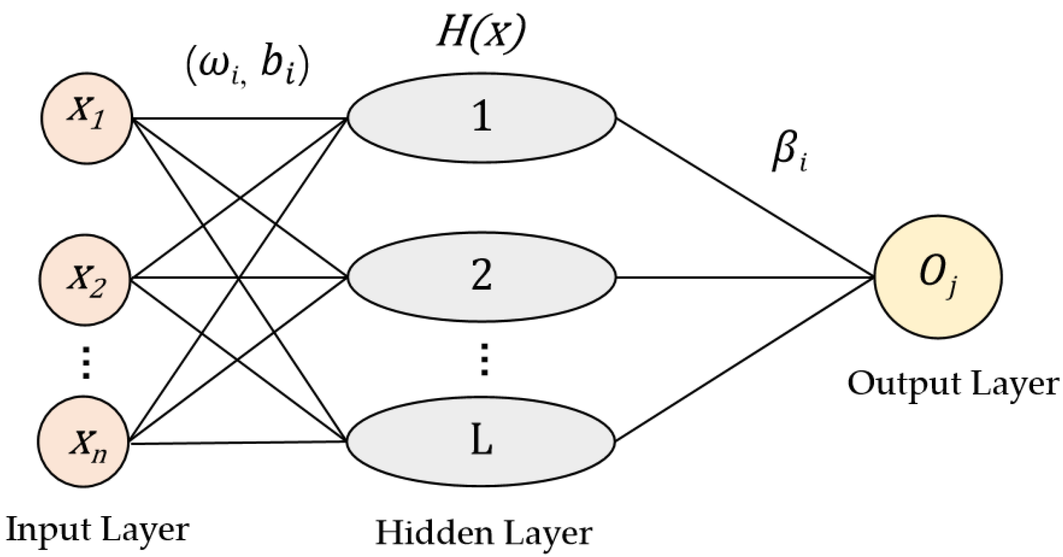
2.4. Extreme Learning Machine

The Extreme Learning Machine (ELM) is an innovative and efficient learning algorithm designed for Single Hidden Layer Feedforward Neural Networks (SLFNs). This approach allows for the random initialization of input weights and biases, thereby facilitating the subsequent determination of the corresponding output weights.

In the context of a single hidden layer neural network, the configuration is illustrated in a scholarly and technical manner in Figure 3, assuming there are N arbitrary samples $(x_i,t_i)$, where $x_i=[x_{i1},x_{i2},\cdots ,x_{in}{]}^T\in R^n$ and $t_i={\left[t_{i1},t_{i2},\cdots ,t_{im}\right]}^T\in R^m$. A single-hidden layer neural network with L hidden nodes can be represented as [27]:

$$\sum _{i=1}^L{\beta }_{i}g\left(w_i\cdot x_j+b_i\right)=o_j,j=1,\cdots ,N$$

(25)

where $w_i=[w_{i,1},w_{i,2},\cdots ,w_{i,n}{]}^T$ is the matrix of input weights, ${\beta }_i$ is the bias vector associated with the hidden layer, and $b_i$ corresponds to the bias of the i-th neuron within the hidden layer. The expression $w_i\cdot x_j$ denotes the scalar product of vectors $w_i$ and $x_j$. $g\left(x\right)$ symbolizes the activation function, as shown in the following equation:

$$g\left(x\right)={\displaystyle \frac{1}{1+e^{-x}}}$$

(26)

The objective of learning in a single hidden layer neural network is to minimize the output error, which can be represented as follows:

$$\sum _{j=1}^N\parallel o_j-t_j\parallel =0$$

(27)

${\beta }_i$, $w_i$, and $b_i$ exist such that

$$\sum _{i=1}^L{\beta }_{i}g\left(w_i\cdot x_j+b_i\right)=t_j,j=1,\cdots ,N$$

(28)

The equation can be expressed in matrix form as follows:

$$H\beta =T$$

(29)

where $H$ represents the output of the hidden layer nodes, $\beta$ denotes the vector of output weights, and $T$ signifies the matrix of desired target outputs.

$$\begin{array}{l}H\left(w_1,\cdots ,w_L,b_1,\cdots ,b_L,x_1,\cdots ,x_L\right)\\ ={\left[\begin{array}{c}g\left(w_1\cdot x_1+b_1\right) \cdots g\left(w_L\cdot x_1+b_L\right)\\ \begin{array}{ccc}g\left(w_1\cdot x_2+b_1\right)& \cdots & g\left(w_L\cdot x_2+b_L\right)\\ ⋮& \cdots & ⋮\\ g\left(w_1\cdot x_N+b_1\right)& \cdots & g\left(w_L\cdot x_N+b_L\right)\end{array}\end{array}\right]}_{N\times L}, \beta ={\left[\begin{array}{c}{\beta }_1^T\\ \begin{array}{c}{\beta }_2^T\\ ⋮\\ {\beta }_L^T\end{array}\end{array}\right]}_{L\times m,},T={\left[\begin{array}{c}{T}_1^T\\ \begin{array}{c}{T}_2^T\\ ⋮\\ T_N^T\end{array}\end{array}\right]}_{N\times m}\end{array}$$

(30)

In the pursuit of training a single hidden layer neural network, our objective was to ascertain the optimal input weight matrices ${\widehat{w}}_i$, bias vectors ${\widehat{b}}_i$, and output weight matrix ${\widehat{\beta }}_i$ that ensure the network’s output closely approximates the desired target outputs $T$, thereby minimizing the training error.

$$∥H\left({\widehat{w}}_i,{\widehat{b}}_i\right){\widehat{\beta }}_i-T∥=min∥H\left(W_i,b_i\right){\beta }_i-T∥$$

(31)

In the context provided, where $i=1,\cdots ,L$, this is equivalent to minimizing the loss function.

$$E=\sum _{j=1}^N{\left(\sum _{i=1}^L{\beta }_{i}g\left(w_i\cdot x_j+b_i\right)-t_j\right)}^2$$

(32)

Traditional algorithms predicated on gradient descent methods are adept at resolving optimization problems of this nature; however, they necessitate the iterative adjustment of the entire set of parameters throughout the learning process. In contrast, within the framework of the ELM algorithm, once the input weights $w_i$ and biases $b_i$ of the hidden layer are assigned randomly, the output matrix of the hidden layer, denoted as $H$, becomes uniquely determined. The training of a single hidden layer neural network is thereby transmuted into the solution of a linear system, represented by $H\beta =T$. The output weights can be resolved as $\widehat{\beta }=H^{†}T$, where $H^{†}$ symbolizes the Moore–Penrose pseudoinverse of $H$. It can be demonstrated that the solution obtained is of minimal norm and is unique.

The ELM training algorithm can be summarized as follows:

(1)

Establish the specific structure of the feedforward neural network;

(2)

Randomly set the parameters ${\omega }_i$ and $b_i$ of the feedforward neural network;

(3)

Solve for the minimum norm least squares solution $\beta$ of the output weight matrix $H$.

2.5. HOA-Optimized ELM Classification Model

As previously mentioned, the hidden layer weights and biases of the ELM are randomly assigned at the outset. To further enhance the model’s rapid convergence to the optimal solution, this paper selected the relatively novel and high-performing HOA to iteratively optimize the hidden layer weights w and biases b of the ELM, thereby improving its classification accuracy. The objective of the optimization is to minimize the fitness value. In this study, Equation (25) was chosen as the fitness function to identify a solution that minimizes this function. The optimization approach is outlined as follows:

(1)

Initialize all the initial parameters of the HOA, including the maximum number of iterations, the upper bound of the population U, and the lower bound L;

(2)

Randomly initialize the population, where each individual in the population is composed of a vector of the hidden layer weights and biases of the ELM, and randomly divide the population into two sub-populations;

(3)

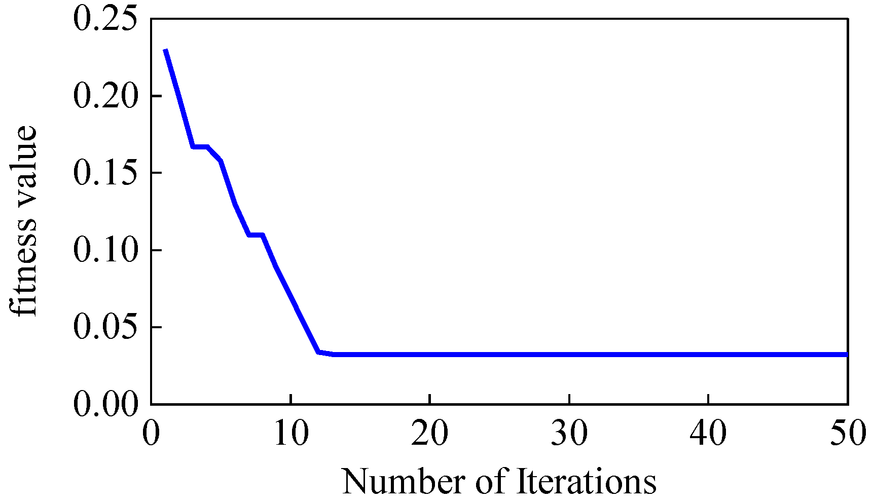
Calculate the fitness value of each individual in the current population according to the fitness function, where the fitness function is Equation (27), and the fitness value is the classification error rate of the training data, recording the individual with the minimum fitness value;

(4)

Update the velocity ${\mathcal{W}}_{i,t}$and position ${\beta }_{i,t+1}$of individuals in the population according to Equations (23) and (24), respectively;

(5)

Repeat steps (3) and (4) until the maximum number of iterations is reached. By following these steps, the optimization of the ELM is achieved. This algorithm is referred to as HOA-ELM in this paper, and its flowchart is presented in Figure 4.

3. Hydropower Unit Fault Diagnosis Model Based on DMD and HOA-ELM

This paper proposes a fault diagnosis model for hydropower units based on DMD and HOA-ELM. Initially, the vibration signals were decomposed using DMD, followed by the extraction and fusion of multi-domain features from the denoised signal, which includes time-domain, frequency-domain, and time-frequency domain features. To simplify the data and address the issue of feature redundancy, PCA was performed for dimensionality reduction. Finally, the extracted features were classified using the HOA-optimized ELM. The specific process is illustrated in Figure 5.

The specific steps of this diagnostic model are as follows:

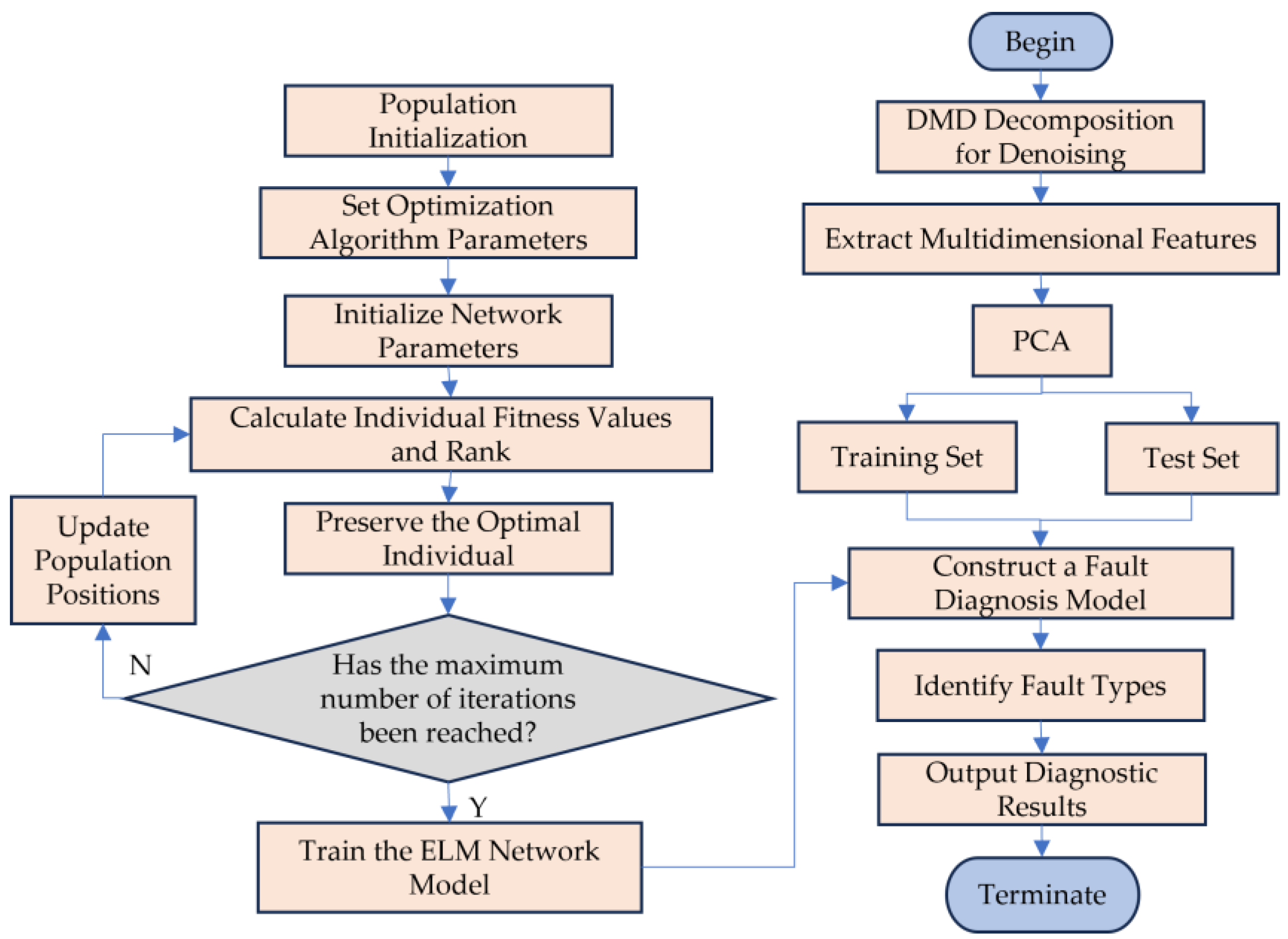
(1)

Perform an adaptive decomposition using DMD on the original signal to obtain a set of IMF arranged in order of frequency, reflecting the features of the signal across different time scales;

(2)

Extract the time-domain and frequency-domain features of the denoised signal, as well as the energy entropy, root mean square, and singular value features of each modal component. Perform PCA on the extracted feature vectors to obtain the reduced-dimensionality feature vectors;

(3)

Utilize the HOA to optimize the hidden layer weights w and biases b of the ELM, and employ the ELM with the optimal parameter configuration obtained as the final classifier for this diagnostic method;

(4)

Input the multi-domain integrated features from step (2) into the optimized ELM from step (3) for fault diagnosis.

4. Case Study Analysis

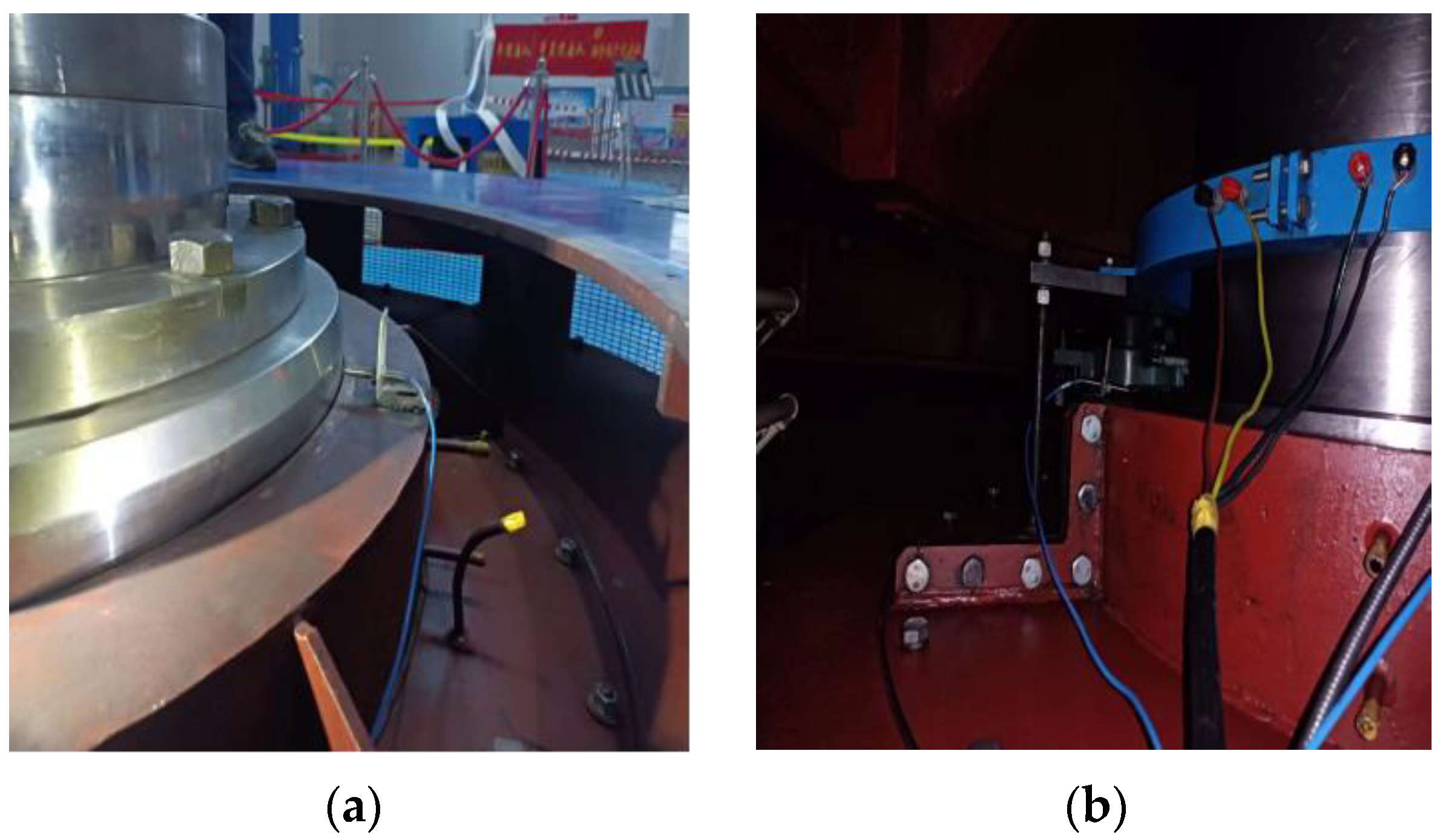
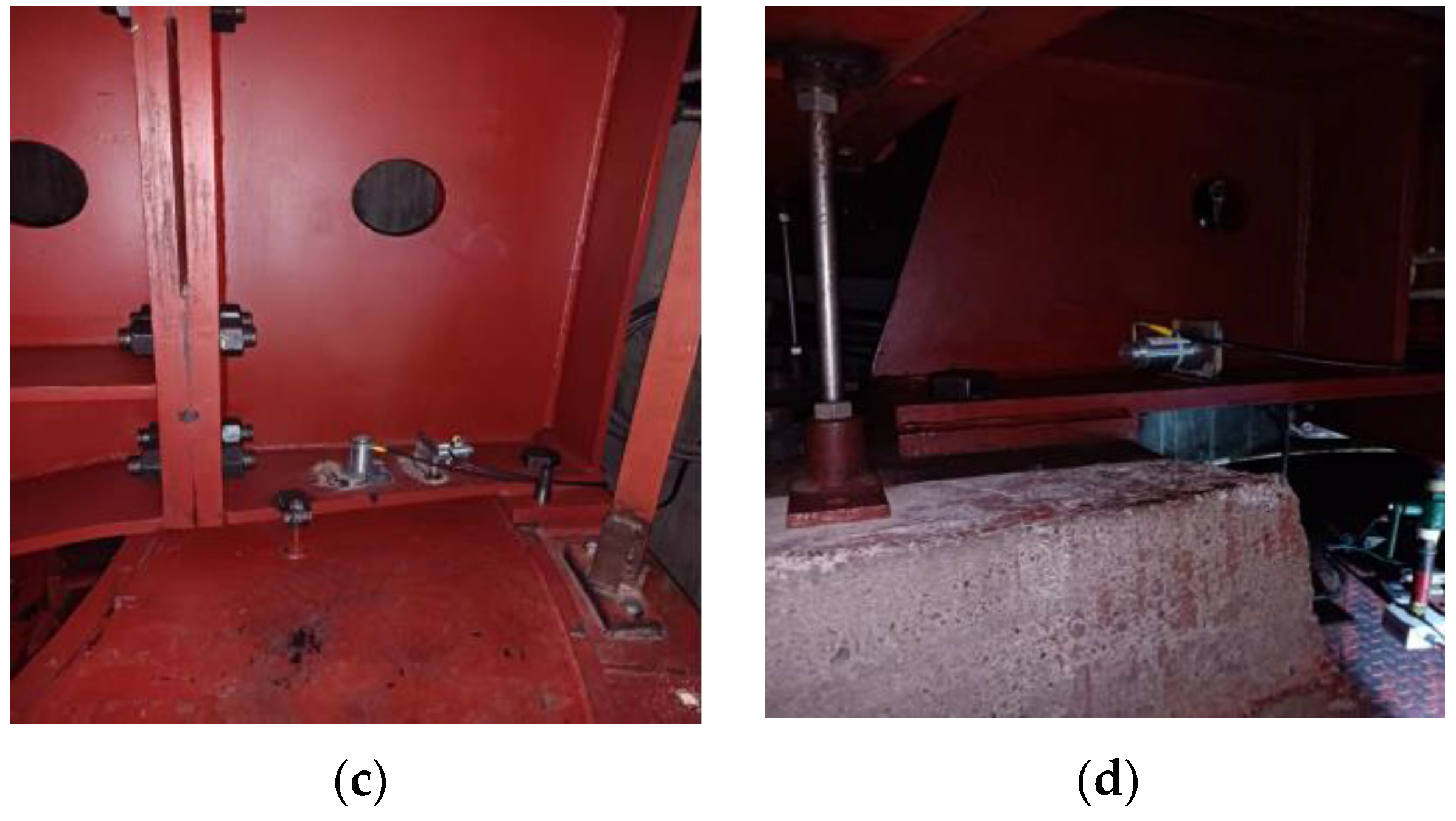
4.1. Data Acquisition

The experimental data for this paper were obtained from sensors installed on various components of the hydropower units within a specific hydroelectric plant. The basic parameters of the hydropower unit are presented in

Table 1. Hydropower unit basic parameters.

Parameter	Value	Unit
Rated Capacity	35	MW
Rated Head	181	m
Rated Flow	25.25	m3/s
Rated Speed	333.3	r/min

.

The primary sensors employed in this study were low-frequency velocity sensors produced by Haoruisi Company (located in Beijing, China). Specifically, the MLS-9H model was used for horizontal measurements, while the MLS-9V model was designated for vertical measurements. These sensors monitored both the upper and lower frames, as well as the cover. To measure rotor swing, we utilized the IN-081 integrated eddy current sensor from the Schenck Company, which is headquartered in Darmstadt, Germany. Furthermore, the 21R series pressure sensors from the KELLER Company, which is headquartered in Baar, Switzerland, are renowned for their high-frequency response and are particularly suitable for pressure pulsation measurements. Figure 6 presents a schematic of the sensor layout.

The collected data were categorized into four operational states as follows: normal, stator–rotor rub, thrust head looseness, and rotor misalignment. For each state, 100 samples were selected and divided into training and testing sets in a 70:30 ratio. The fault labels and the division of sample data are presented in

Table 2. Dataset partitioning.

Operating Condition	Label	Training Set	Test Set
Normal Condition	1	70	30
Stator–Rotor Rub	2	70	30
Thrust Head Looseness	3	70	30
Rotor Misalignment	4	70	30

. The time-domain and frequency-domain graphs for these four operational states are illustrated in Figure 7, Figure 8, Figure 9 and Figure 10.

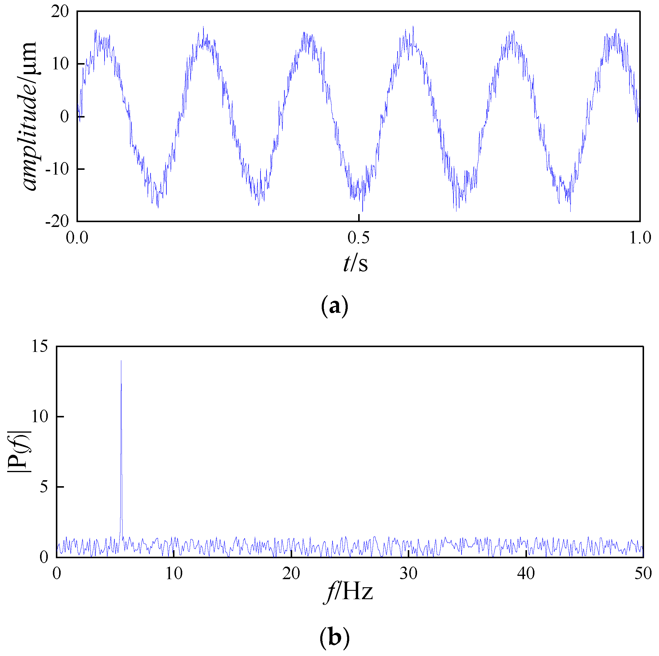
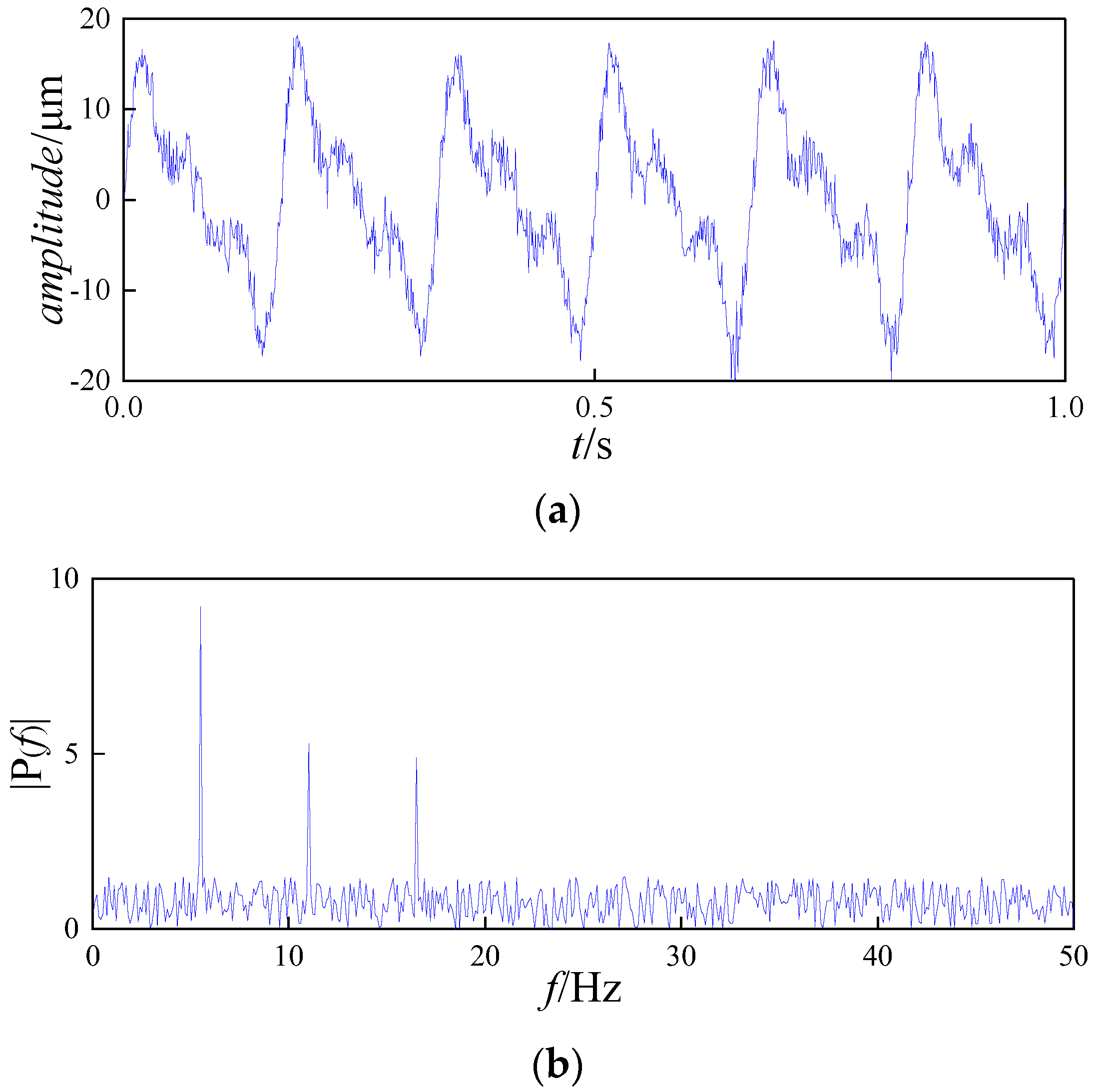
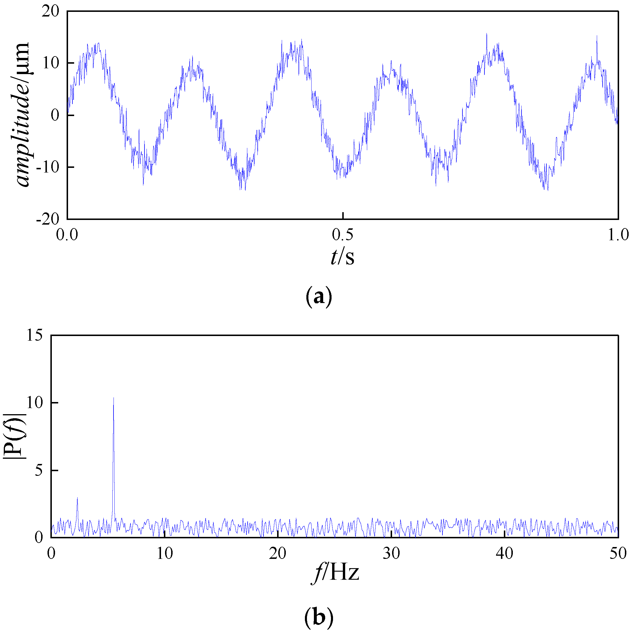
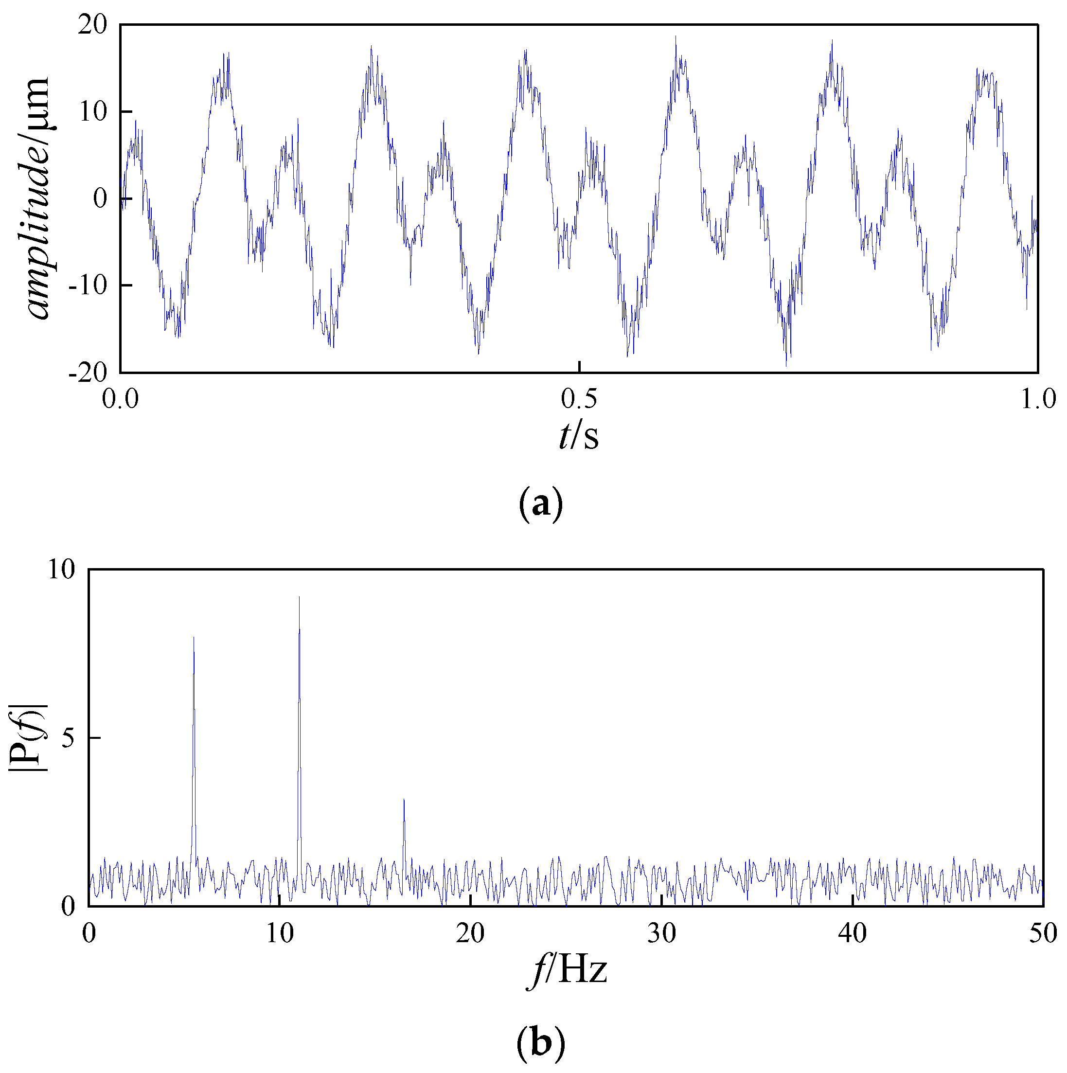
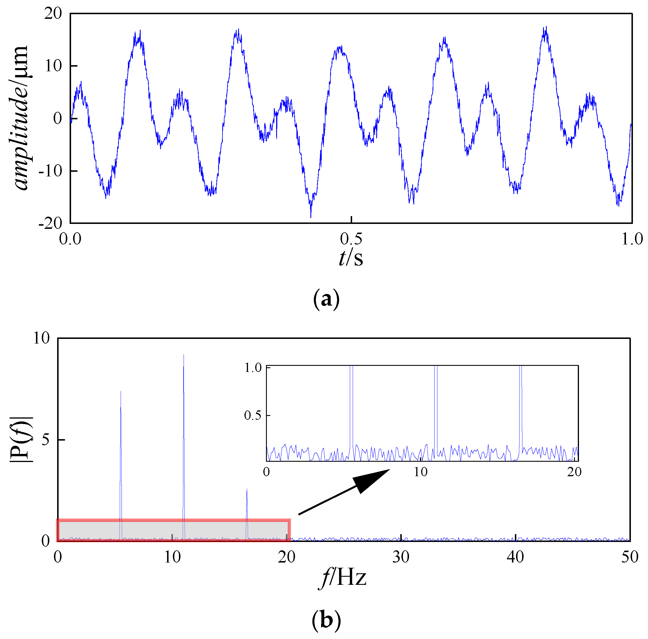
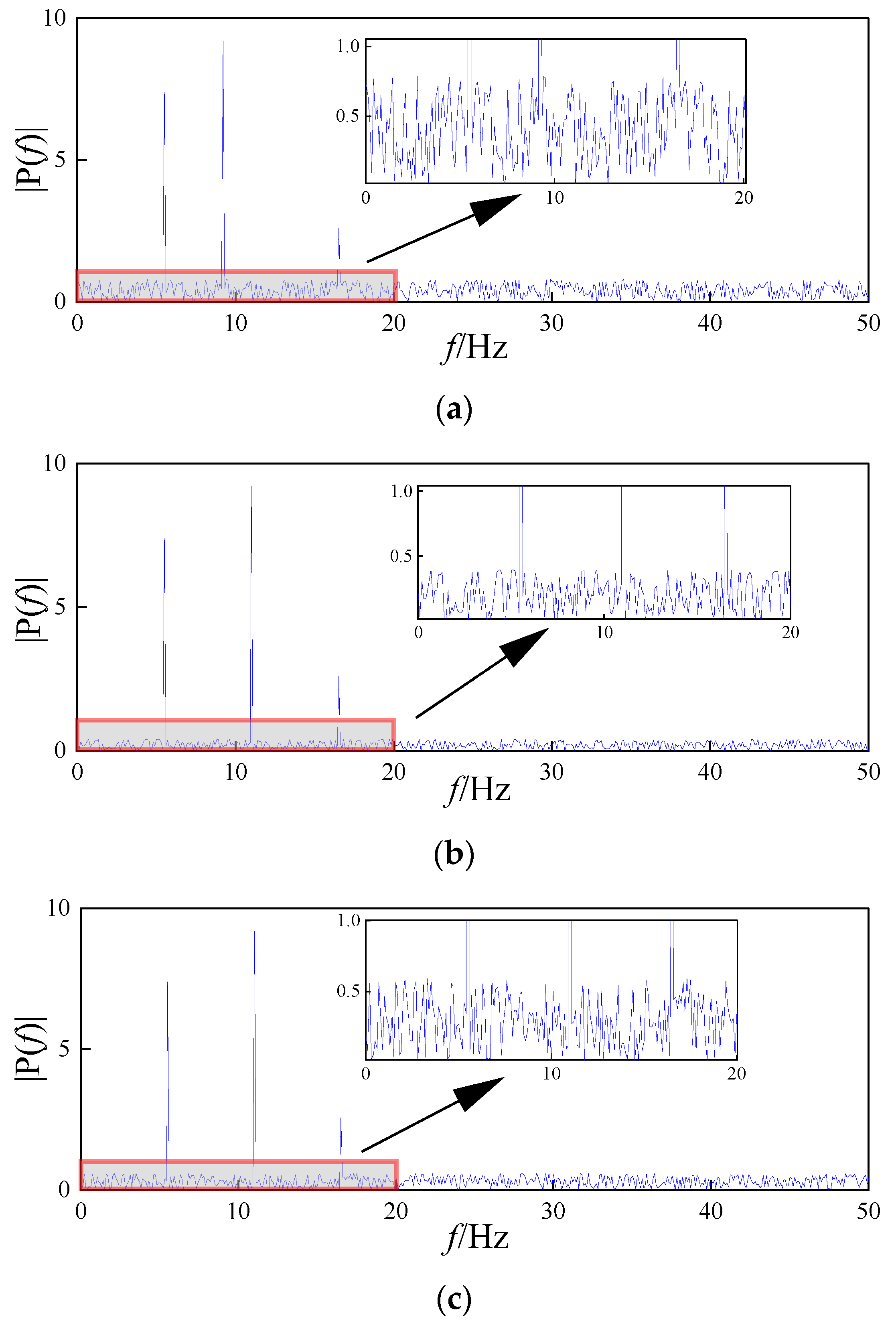
4.2. DMD Decomposition for Noise Reduction

This study uses a set of samples demonstrating rotor misalignment as a case study and employs DMD to decompose the vibration signals into several modal components. The results of this decomposition are illustrated in Figure 11.

Since each IMF component is derived from the decomposition of the original signal, the correlation coefficient between each component and the original signal can indicate its significance. A higher correlation coefficient signifies a greater degree of similarity and a more substantial amount of inherent data. By establishing a threshold, we can select effective IMF components for reconstruction, discard irrelevant components, and achieve noise reduction. Subsequently, the correlation coefficients between each IMF component and the original signal were calculated, along with the threshold. IMF components with correlation coefficients exceeding the threshold were then superimposed for reconstruction. The specific computational results are presented in

Table 3. Calculation results of the correlation coefficients and threshold.

Type	Component	Value
Correlation coefficient	IMF1	0.627
	IMF2	0.56
	IMF3	0.459
	IMF4	0.203
	IMF5	0.175
Threshold	0.27

.

Upon calculation, a threshold of 0.27 was established, resulting in the exclusion of the IMF4 and IMF5 components. The IMF1, IMF2, and IMF3 components were then reassembled to achieve noise reduction. The time–frequency waveform of the denoised signal is illustrated in Figure 12.

As illustrated in Figure 12, the denoising methodology presented here effectively eliminates the majority of noise components. The vibration signal waveform after denoising exhibits more pronounced and discernible characteristics compared with its pre-denoising state. Furthermore, the denoised signal maintains a high level of fidelity to the original signal in terms of overall characteristics and peak values. Spectrally, the energy of the vibration signal post-denoising is more concentrated, facilitating more accurate identification and analysis of the signal’s frequency features. To further validate the superiority of the DMD method, this paper conducted comparative experiments, contrasting it with other noise reduction algorithms such as EMD [28], EEMD [29], and Empirical Wavelet Transform (EWT) [30]. The results are illustrated in Figure 13.

To assess the comparative efficacy of various denoising methods quantitatively, this study employed the following metrics: the Roughness of Variance Ratio (RVR) [31] and the Noise Metric (NM) [32]. The RVR indicates the smoothness of the signal after denoising, with values approaching zero signifying greater smoothness. Conversely, the NM reflects the change in energy before and after denoising, with higher values suggesting superior denoising performance. The evaluation metrics for each denoising method are summarized in

Table 4. Comparative analysis of denoising algorithms.

Denoising Algorithm	RVR	NM
DMD	0.138	10.376
EMD	0.214	9.735
EEMD	0.157	10.043
EWT	0.179	9.872

.

As demonstrated in Table 4, the method proposed in this paper achieves a higher NM value and an RVR value closer to zero after denoising. This indicates greater signal energy, enhanced smoothness, and improved denoising results. These findings suggest that the method outlined in this paper exhibits commendable denoising capabilities and is well-suited for the analysis of vibration signals in hydropower units.

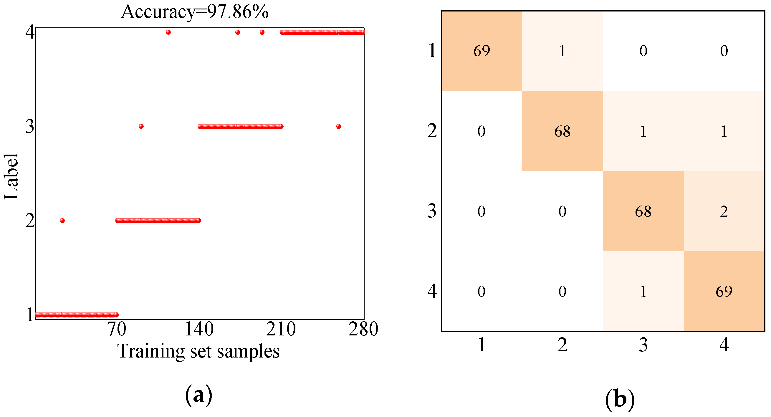
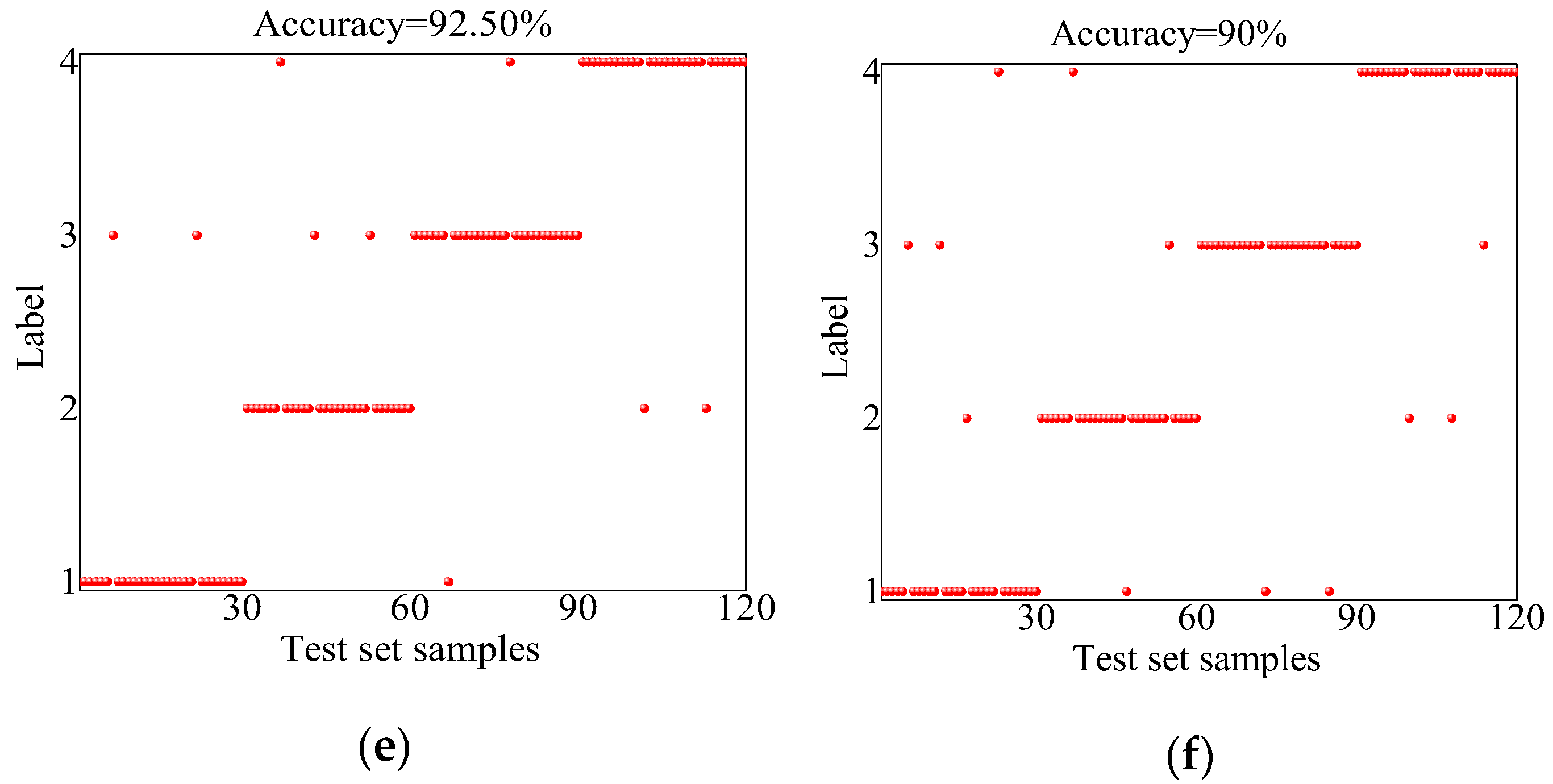
4.3. HOA-ELM Diagnostic Model

By applying DMD to the raw signal for denoising, multidimensional features were extracted from the denoised signal. PCA was then utilized for dimensionality reduction, and the resulting feature vectors were input into an ELM for fault classification. To enhance the classification performance of the ELM model, the HOA was employed to optimize the hidden layer weight w and bias b parameters. In this study, the population size was set to N = 30, and the maximum number of iterations was T = 50, with the training set’s error rate serving as the fitness function. As illustrated in Figure 14, which depicts the convergence process of the HOA optimization algorithm, the fitness value converges to 0.0324 after 13 iterations, yielding the optimized parameters w = 0.643 and b = 0.427.

This paper began by training the fault diagnostic model, employing the optimized parameters obtained from the HOA as inputs for the ELM. The resulting diagnostics are illustrated graphically in Figure 15. Following this, a quantitative evaluation of the model’s performance was conducted using the established metrics of precision [33], recall [34], and accuracy. The detailed analytical findings from the training dataset are presented in

Table 5. Diagnostic result evaluation metrics for the training set.

Evaluation Metric	Label				Mean Value
	1	2	3	4
Precision	100%	98.55%	97.14%	95.83%	97.88%
Recall	98.57%	97.14%	97.14%	98.57%	97.86%
Accuracy	97.86%

.

The diagnostic results from the training set indicate that the model proposed in this paper achieved an accuracy rate of 97.86%. This demonstrates that the optimal parameter solution identified by optimizing the ELM with the HOA can yield effective training results, resulting in a model with exceptional classification performance. Consequently, this model can be effectively applied to the fault diagnosis of hydropower units. The training set comprised 70 samples for each operating condition, totaling 280 samples. The diagnosis for both normal conditions and rotor misalignment conditions achieved an accuracy rate of 98.57%. In contrast, the accuracy rate for diagnosing the stator–rotor rub condition and the thrust head loosening condition was slightly lower, yet it still reached 97.14%.

To validate the diagnostic effectiveness, the test set was input into the well-trained HOA-ELM model. To further assess the superiority of the diagnostic model presented in this paper, comparisons were initially made with diagnostic models that simultaneously optimize the Support Vector Machine (SVM) [35] and Backpropagation (BP) [36] using the HOA. Subsequently, comparisons were conducted with diagnostic models that optimize the ELM using the Sparrow Search Algorithm (SSA) [37] and the Grey Wolf Optimizer (GWO) [38], as well as with diagnostic models that do not employ optimization algorithms. The specific diagnostic results are illustrated in Figure 16, while the comparative analysis of diagnostic model accuracies is shown in Figure 17.

In the figure, it is evident that the diagnostic model presented in this paper misclassified five samples, resulting in an accuracy rate of 95.83%. This performance can be attributed to PCA, which enhanced training efficiency and addressed the issue of feature redundancy. Additionally, the HOA successfully identified more optimal initial parameters for the ELM model. Because of the ELM’s robust generalization capabilities, it can be effectively applied to previously unseen data, making it particularly advantageous in practical applications. Compared with the HOA-BP and HOA-SVM diagnostic models, the accuracy rates increased by 4.54% and 1.76%, respectively. The SSA-ELM, GWO-ELM, and traditional ELM diagnostic models achieved accuracy rates of 93.33%, 92.50%, and 90%, respectively. The accuracy rate of the HOA-ELM model exceeded these models by 2.68%, 3.60%, and 6.48%, respectively, indicating that the HOA model possesses superior optimization capabilities and a faster convergence speed.

5. Conclusions

This paper proposes a fault diagnosis method for hydropower units based on DMD and HOA-ELM, and the experimental results confirm the following conclusions:

(1)

To address the problem of noise interference in the vibration signals of hydropower units, this paper utilizes DMD and reconstructs the signal using a thresholding technique to mitigate noise. A comparative analysis with alternative noise reduction methods demonstrates that the signal processed with the proposed noise reduction technique exhibits higher energy levels and smoother characteristics, indicating more effective noise reduction.

(2)

To address the randomness of the weights and biases in the ELM, an HOA with improved convergence performance is introduced to optimize these two parameters. Experimental comparisons demonstrate that the HOA significantly enhances the model’s classification accuracy to 95.83%, representing a 6.48% increase over the traditional ELM model.

(3)

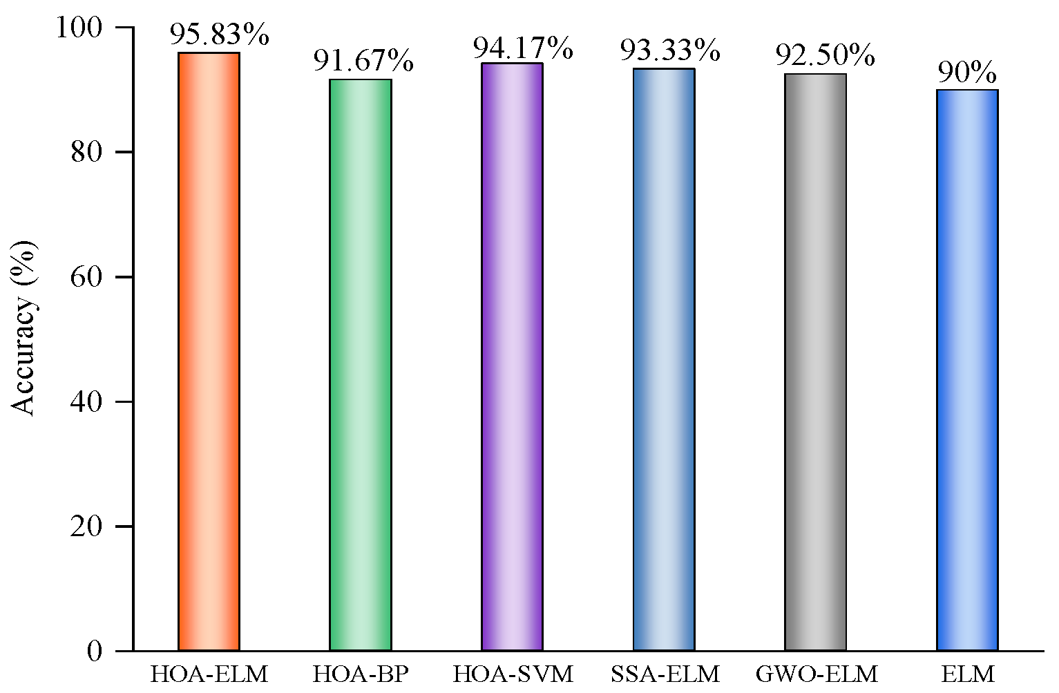
A comparison of unit status recognition among six models, including HOA-ELM, demonstrates that the proposed model achieves the highest diagnostic accuracy. This confirms that the HOA-ELM model is an effective hydropower unit fault diagnosis tool with excellent diagnostic precision.

However, this model is specifically designed for the classification and identification of vibration-related faults and is not suitable for non-vibration-related faults in hydropower units. Furthermore, the HOA has limitations in balancing global and local search capabilities. To address these limitations, researchers may need to refine the HOA or integrate it with other algorithms to enhance its performance and robustness across various applications. This will be a key area for future research.

References

- You, P.; Ji, H.; Tang, W. Vibration analysis of giant hydro-generator sets. Hydropower New Energy 2021, 35, 35–38. [Google Scholar]
- Liu, Y.; Liu, W.; Shi, Y. GMM-DBSCAN multi-scale cleaning of vibration signals from hydropower units in complex operating conditions. J. Hydroelectr. Eng. 2022, 41, 153–162. [Google Scholar]
- Hu, X.; Xiao, Z.; Liu, D. Vibration fault identification method of hydropower unit based on EEMD-SDCC-HMM. J. Vib. Shock 2022, 41, 165–175+230. [Google Scholar]
- Jia, J.; Wu, M.; Song, K. Traction network overvoltage identification based on short time Fourier transform and deep learning. Electr. Eng. 2021, 22, 1–10. [Google Scholar]
- Ji, L.; Jing, X.; Zhou, D. Fault diagnosis of hydropower unit based on VMD-WT-CNN and attention mechanism. Sci. Hydropower Energy 2024, 42, 184–187+157. [Google Scholar]
- Wu, K.; Zhou, J.; Pan, W. Research on prediction method of measured swing signal for hydro turbine unit based on EMD-LSTM model. Sci. Hydropower Energy 2024, 42, 179–182. [Google Scholar]
- Wang, M.; Weng, S.; Yu, X. Structural damage identification based on time-varying modal mode shape of wavelet transformation. J. Vib. Shock 2021, 40, 10–19. [Google Scholar]
- Wang, X.; Niu, S.; Zhang, K. Image fusion of infrared weak-small target based on wavelet transform and feature extraction. J. Northwestern Polytech. Univ. 2020, 38, 723–732. [Google Scholar] [CrossRef]
- Zhou, X.; Tong, X. Ultra-short-term wind power combined prediction based on CEEMD-SBO-LSSVR. Power Syst. Technol. 2021, 45, 855–864. [Google Scholar]
- Schmid, P.J. Dynamic mode decomposition of numerical and experimental data. J. Fluid Mech. 2010, 656, 5–28. [Google Scholar] [CrossRef]
- Chen, C.; Zou, Z.; Zou, L. Time series prediction of ship maneuvering motion in waves based on high-order dynamic mode decomposition. China Shipbuild. 2023, 64, 216–224. [Google Scholar]
- Li, J.; Hu, X.; Geng, J. Fault diagnosis method for variable working condition bearings based on DMD and improved capsule network. J. Electr. Mach. Control 2023, 27, 48–57. [Google Scholar]
- Yang, T.; Wang, W.; Zhang, P. Fault diagnosis method for hydropower unit based on CEEMDAN and hybrid grey wolf optimization algorithm optimized SVM. Sci. Hydropower Energy 2022, 40, 195–198. [Google Scholar]
- Hu, X.; Xiao, Z.; Liu, D. Hydropower unit fault diagnosis based on VMD-CNN. J. Hydroelectr. Eng. 2020, 38, 137–141. [Google Scholar]
- He, K.; Chen, J.; Jin, Y. Application of EEMD multiscale entropy and ELM in feature extraction of vibration signal of hydropower unit. China Rural Water Hydropower 2021, 176–182+187. [Google Scholar] [CrossRef]
- Liu, W.; Zheng, Y.; Ma, Z. An intelligent fault diagnosis scheme for hydropower units based on the pattern recognition of axis orbits. Measure. Sci. Technol. 2023, 34, 025104. [Google Scholar] [CrossRef]
- Li, X.; Xu, Z.; Wang, Y. PSO-MCKD-MFFResnet based fault diagnosis algorithm for hydropower units. Math. Biosci. Eng. 2023, 20, 14117–14135. [Google Scholar] [CrossRef]
- Chen, Q.; Wei, H.; Rashid, M. Kernel extreme learning machine based hierarchical machine learning for multi-type and concurrent fault diagnosis. Measurement 2021, 184, 109923. [Google Scholar] [CrossRef]
- Zhang, J.; Zhang, Q.; Qin, X. A two-stage fault diagnosis methodology for rotating machinery combining optimized support vector data description and optimized support vector machine. Measurement 2022, 200, 111651. [Google Scholar] [CrossRef]
- Zheng, J.; Wei, G. Time-frequency and energy analysis of electromagnetic signals based on multi-resolution dynamic mode decomposition. Syst. Eng. Electron. Technol. 2022, 44, 1468–1474. [Google Scholar]
- Ye, H.; Zhong, H.; Ou, Y. A denoising method for tunnel blasting vibration signals based on VMD and energy entropy. Met. Mines 2022, 1–17, submitted for publication. [Google Scholar]
- Huo, H.; Chen, G.; Wang, W. Benchmark solution for the random vibration response of moderately thick cylindrical shells under steady/non-steady excitation. Acta Mech. Sin. 2022, 54, 762–776. [Google Scholar]
- Zi, Y.; Zhou, J. Fault diagnosis of rolling bearings based on S-transform and singular value median decomposition. J. Mech. Electr. Eng. 2022, 39, 949–954. [Google Scholar]
- Zhang, Y.; Tian, L. Comprehensive evaluation of thermal power unit operation based on PCA and improved TOPSIS method. J. North China Electr. Power Univ. Nat. Sci. Ed. 2023, 50, 110–116+126. [Google Scholar]
- Zhu, X.; Yuan, Z.; Li, H. A deformation prediction method for concrete dams based on BP-PCA-WCA-SVM. Yangtze River Sci. Acad. 2024, 41, 138–145. [Google Scholar]
- Oladejo, S.O.; Ekwe, S.O.; Mirjalili, S. The Hiking Optimization Algorithm: A novel human-based metaheuristic approach. Knowl. Based Syst. 2024, 296, 111880. [Google Scholar] [CrossRef]
- Zhang, N.; Zhu, Y.; Sun, N. Vibration trend prediction of hydropower unit based on OVMD-TVFEMD secondary decomposition and HPO-ELM. Sci. Hydropower Energy 2023, 41, 204–207+199. [Google Scholar]
- Yao, F.; Yang, X.; Ding, F. Fault diagnosis of rolling bearing based on wavelet threshold noise reduction EMD-AR spectrum analysis and extreme learning machine. Manuf. Technol. Mach. Tool 2023, 7, 16–20+31. [Google Scholar]
- Xiao, B.; Zeng, Y.; Dao, F. Fault sound pattern recognition model for hydropower unit rubbing fault based on EEMD-CNN. J. Hydroelectr. Eng. 2024, 43, 59–69. [Google Scholar]
- Zhang, H.; Zhu, Y.; Lv, M. Bearing fault identification based on MCKD denoising and improved EWT signal decomposition. Mech. Des. Res. 2023, 39, 80–83+91. [Google Scholar]
- Wang, W.; Hou, K.; He, K. Fault diagnosis of hydropower unit based on GSA optimized VMD-DBN. J. Wuhan Univ. Eng. Ed. 2023, 56, 244–250. [Google Scholar]
- Xu, Z.; Liu, T.; Ren, S. Fault diagnosis of hydropower unit based on time-delayed multi-scale fluctuation dissipation entropy and improved kernel extreme learning machine. Eng. Sci. Technol. 2024, 56, 41–51. [Google Scholar]
- Zhang, F.; Yuan, F.; He, Y. Denoising of hydropower unit vibration signals based on NLM-CEEMDAN and sample entropy. China Rural Water Hydropower 2023, 6, 286–294. [Google Scholar]
- Chen, F.; Wang, B.; Zhou, D. Fault diagnosis method for shaft fault of hydropower unit by integrating improved symbolic dynamic entropy and random configuration network. J. Hydraul. Eng. 2022, 53, 1127–1139. [Google Scholar]
- Li, Z.; Lin, H.; Xu, X. Fault detection method for turbine unit based on KPCA-PSO-SVM. J. Drain. Irrig. Mach. Eng. 2023, 41, 467–474. [Google Scholar]
- Li, X.; Qian, J.; Zeng, Y. Fault diagnosis of hydropower unit based on UPEMD fusion RCMCSE and ALWOA-BP. J. Hydraul. Eng. 2024, 55, 744–755. [Google Scholar]
- Xu, J.; Yang, P.; Yin, X. Gear fault diagnosis based on EMD decomposition and Levy-SSA-BP neural network. Mech. Transm. 2024, 48, 152–157. [Google Scholar]
- Chen, Q.; Liao, H.; Sun, Y. Prediction of photovoltaic power generation based on GWO-GRU. Acta Sol. Energy 2024, 45, 438–444. [Google Scholar]