Article

A Method for Evaluating Demand Response Potential of Industrial Loads Based on Fuzzy Control

1
Energy Development Research Institute of China Southern Power Grid, Guangzhou 510663, China
2
Beihai Power Supply Bureau Guangxi Power Grid Co., Ltd., Beihai 536000, China
*
Author to whom correspondence should be addressed.
Energies 2024, 17(20), 5146; https://doi.org/10.3390/en17205146
Submission received: 12 July 2024 / Revised: 2 October 2024 / Accepted: 9 October 2024 / Published: 16 October 2024
(This article belongs to the Section K: State-of-the-Art Energy Related Technologies)

Abstract

:
Demand response (DR) can ensure electricity supply security by shifting or shedding loads, which plays an important role in a power system with a high proportion of renewable energy sources. Industrial loads are vital participants in DR, but it is difficult to assess DR potential because of many complex factors. In this paper, a new method based on fuzzy control is given to assess the DR potential of industrial loads. A complete assessment framework including four steps is presented. Firstly, the industrial load data are preprocessed to mitigate the influence of noisy and transmission losses, and then the K-means algorithm considering the optimal cluster number is used to calculate baseline load of industrial load. Subsequently, an open-loop fuzzy controller is designed to predict the response factor of different industrial loads. Three strongly correlated indicators, namely peak load rate, electricity intensity, and load flexibility, are selected as the input of fuzzy control, which represents response willingness. Finally, the baseline load of diverse clustering scenarios and the response factor are used to calculate the DR potential of different industrial loads. The proposed method takes into account both economic and technical factors comprehensively, and thus, the results better represent the available DR potential in real-world situations. To demonstrate the effectiveness of the proposed method, the case of a medium-sized city in China is studied. The simulation focuses on the top eight industrial types, and the results show they can contribute about 189 MW available DR potential.

1. Introduction

As fossil energy consumption intensifies alongside growing low-carbon awareness, the share of renewable energy in energy systems is expected to progressively rise annually. In alignment with the “Double Carbon” strategy, the Chinese government has proposed the construction of a novel power system, wherein new energy takes center stage [1]. Nevertheless, the intermittency of renewable energy gives rise to a series of challenges on the power grid, such as electricity supply security and power system operation [2]. As the proportion of thermal power decreases, the importance of regulating resources on demand side become more pronounced [3]. The primary objective of DR is to change electricity consumption habits through electricity price or incentive policy [4]. It plays a key role in mitigating peak loads and promoting the consumption of new energy [5]. Therefore, DR is receiving increasing attention in China and has broad application prospects [6].
Potential assessment is the foundation for implementing demand response, which is also closely related to power grid planning and operation [7]. Some solutions have been achieved in the literature. Through the assessment of various resident types via a questionnaire survey, the willingness of diverse users to participate in DR can be ascertained [8]. In the literature [9], an analysis of the correlation between energy consumption, income and engagement in DR is conducted utilizing household income surveys. The adjustable DR potential in the region is subsequently evaluated based on the above solution. However, the method of a questionnaire survey exhibits substantial limitations, characterized by time-consuming processes, intensive workloads, and challenges in assessing changes in user DR potential. The literature [10], utilizing the economic utility function, delves into the modeling of household user response behavior. However, obtaining user-specific price elasticity and power consumption characteristics is challenging and is significantly influenced by regional and temporal factors, rendering it less practical. In reality, commercial and residential users exhibit limited individual adjustability and face challenges in aggregation [11]. This inherent limitation hinders the effective realization of theoretical potential in practical implementation. The core principle underlying the adjustable potential assessment of DR for power users lies in establishing the connection between user characteristic information and response labels. Notably, among diverse user types, industrial users stand out due to their substantial adjustable potential arising from significant electricity consumption and relatively stable process flows [12]. Consequently, a more precise assessment of available DR potential can be achieved through an in-depth analysis of pertinent characteristics specific to industrial users.
In recent years, a novel approach using artificial intelligence algorithms [13,14,15] has been introduced for DR potential assessment. Grounded in the long short-term memory neural network, a study [14] introduces a methodology for predicting the adjustable potential of DR, hinging on the elastic incentive price. In [15], a combination of reinforcement learning and the regional randomization method is employed to assess the potential of electric water heaters. While these assessment schemes effectively address the issue of limited data in the initial stages of DR, offering valuable insights for the current DR adjustable potential assessment in China, they nonetheless neglect the variations in DR characteristics among different users.
Current studies focus on theoretical DR potential [16], technical DR potential [17], and economic DR potential [18]. However, there is a scarcity of research on available DR potential. Indeed, the adjustable DR potential of industrial users is also impacted by users’ participation willingness [19]. The assessment of available DR potential can be indirectly carried out by computing the response factor across different industries. However, establishing a DR model for diverse users within distinct industries poses challenges and is not easily subjected to quantitative analysis. Traditional forecasting methods often need accurate data and clear logical relations but may be inadequate in the face of incomplete information. Fuzzy logic provides an effective means to deal with this uncertainty, allowing us to use fuzzy sets and fuzzy rules to construct prediction models. Fuzzy control [20] represents a control methodology grounded in fuzzy logic, widely applied across various fields [21,22,23]. The fundamental concept involves incorporating fuzzy input and output, defining fuzzy rules without establishing explicit mathematical models. Consequently, the introduction of the fuzzy control concept is proposed for the assessment of available DR potential.
This paper introduces a novel method to evaluate the available DR potential of industrial loads by integrating baseline loads and response factors. A fuzzy controller is specifically designed to predict the response factor, leveraging three key indicators strongly associated with response willingness as input. The proposed method comprehensively considers economic and technical factors and can better reflect available DR potential.

2. DR Potential Assessment Framework

The DR potential assessment framework includes four steps as shown in Figure 1. Step 1 is to preprocess the load data. To eliminate the impacts of noise and transmission losses, Kalman filtering (KF) is applied to the load data of diverse industries [24], and an interpolation technique is used to handle the missing data.
Step 2 is to obtain the baseline load of industrial user. In a year, an industrial user may have different production scenarios, and the response factor for each production scenario may be different. Therefore, the K-means algorithm is applied to obtain the typical load baselines of different scenarios, and each clustering result represents a typical load baseline. The optimal cluster number of typical load baselines is determined utilizing the Elbow Method [25] and Silhouette Coefficient Index [26].
Step 3 is to predict the DR factor for each typical load baseline. A fuzzy controller is designed to predict the response factor of different industrial loads. Three strongly correlated indicators including peak load rate, electricity intensity and load flexibility are selected as the inputs.
Step 4 is to calculate the available DR potential utilizing the baseline load and the response factor of different clustering scenarios.
Step 2, step 3 and step 4 will be illustrated in details in Section 3, Section 4 and Section 5, respectively. The key variables of the proposed method are shown in Table 1.

3. Baseline Load Calculation

Industry sectors often display diverse load characteristics driven by factors such as production orders, holidays and seasonal variations in a year, which must be considered during accessing DR potential. Consequently, appropriate classification is used to derive the typical load baseline of different scenarios. The K-means clustering algorithm operates as a partition-based clustering approach, utilizing distance as the similarity measure between data [27]. The clusters number k represents the number of typical load scenarios.
Given a load dataset of fi(t), k-means aims to partition the total days’ data into k clusters, with each cluster containing nij days’ data. Therefore, through K-means algorithm, we can obtain the following results:
P i j , n i j = k m e a n s ( f i ( t ) , k )
where k is the cluster number, Pij is the typical load of cluster j, and nij is the data number of the cluster j.
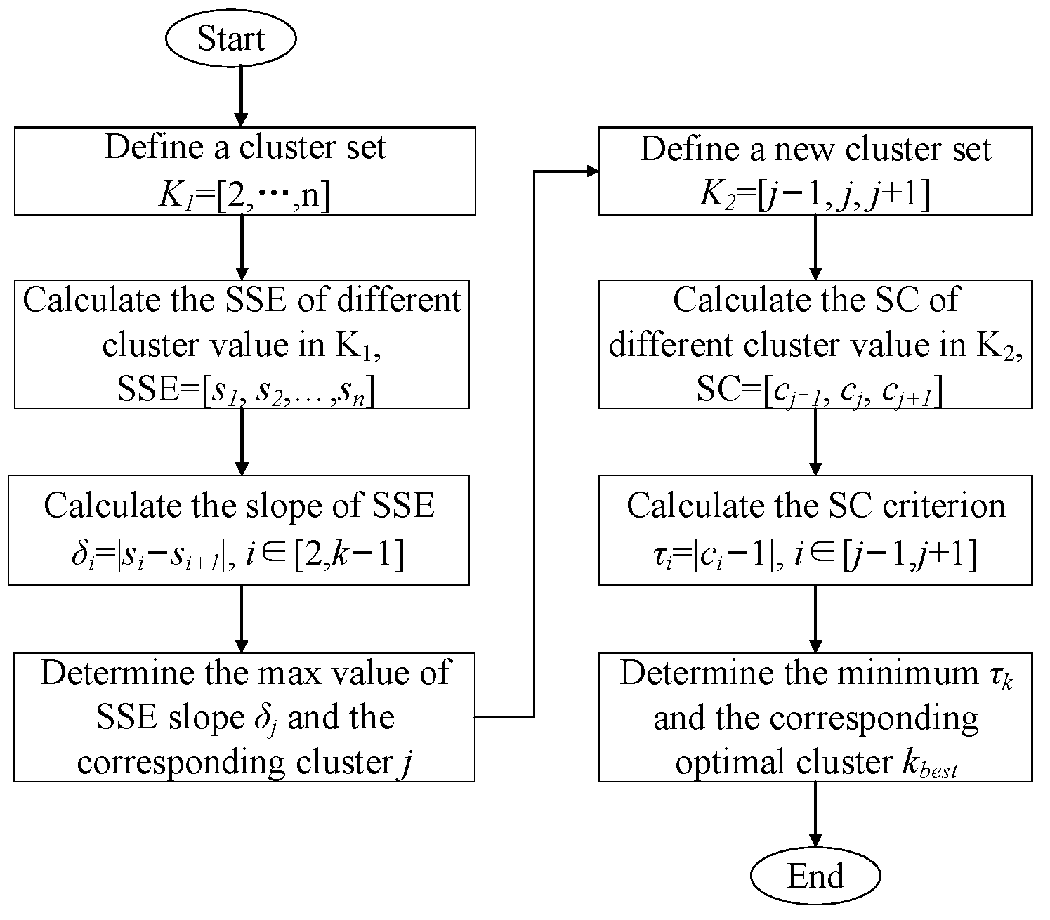
The cluster number k is a key parameter for classification results, and the Elbow Method and Silhouette Coefficient2 are used to comprehensively ascertain the optimal k value in this paper as shown in Figure 2.
The Elbow Method serves as a clustering effect analysis technique employed to ascertain the optimal value of k. Within the K-means clustering algorithm, the Elbow Method determines the best k value by computing the intra-cluster sum of squares (SSE) under various k values. The SSE is calculated by obtaining the SSE corresponding to different k values and observing the trend in SSE change with k values. When the k value increases to a certain extent, the decline speed of SSE significantly slows down, resulting in an “inflection point” recognized as the “Elbow” of the Elbow Method. The optimal k range is proximate to the k value associated with the elbow. The SSE is calculated as follows:
S S E = d i s t ( d i , ψ ) 2
where dist represents the distance, di represents the ith data, and ψ represents the center point of di data.
The Silhouette Coefficient serves as an evaluation index for clustering density and dispersion. The closer the value is to 1, the more optimal the clustering.
S C = δ φ / max ( φ , δ )
where SC is the Silhouette Coefficient, φ is the mean distance between samples in the same cluster and each other, and δ is the mean distance between samples and samples in the nearest cluster except its own cluster.
Firstly, K-means is used to classify two to n clusters, and the SSE and SC of different clusters are also calculated. The optimal cluster number will be determined by the SSE and SC values. Based on the optimal cluster number, the proportion between the baseline load of different clustering scenarios and the number of days of the scenario is calculated, which is convenient for the subsequent classification and calculation of the peak load rate corresponding to the baseline load of different scenarios. Then, the corresponding response factor of the scene is calculated and the response factor of the industry is obtained by equal proportion conversion. The optimal number of clusters is selected as shown in Figure 2.

4. Response Factor Based on Fuzzy Controller

4.1. Input Data Analysis

The response factor represents the willingness and ability of diverse industrial users to participate in DR. Three indicators—electricity intensity, peak load rate, and load flexibility—are utilized as inputs to the fuzzy controller, which represent the influence of economy, technology and response time, respectively.
(1)
Electricity Intensity
To reflect the response willingness, the concept of electricity intensity α was proposed in the literature [19]. The electricity intensity represents GDP per kWh. It has to do with the willingness to respond and reflects the users’ sensitivity to electricity prices. A lower electricity intensity corresponds to higher response willingness. It is important to note that electricity intensity is not a fixed value; rather, it is influenced by factors such as product prices within the industry, production technology levels, and electricity prices in the region. Electricity intensity α is defined as follows:
α i = ρ i / ζ i
where ρi is the GDP of industrial user i, and ζi is the annual electricity consumption of users in the industry.
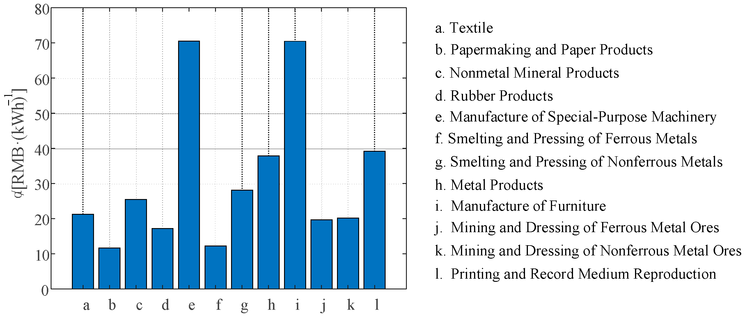
Acquiring product sales data from users may pose challenges due to confidentiality concerns. However, the electricity intensity of different users within the same industry exhibits high similarity. In practical assessments, the industry’s typical value can be employed for calculations. Taking the data of Guangdong Province in China as an example [28], the electricity intensity of various industries is displayed in Figure 3.
(2)
Peak load rate
To reflect the relation between the response time and peak load of industries, this paper proposes the concept of peak load rate β. The DR factor is influenced by the user’s electricity consumption habits. If the peak load occurs within the DR period, the response factor is high, indicating user’s strong response ability; otherwise, it is low. The DR time can be determined based on the region’s peak load. Assuming the DR period is t1t2, the peak load rate β is calculated as follows:
β i j = max P i j t max f i ( t ) t t 1 , t 2
(3)
Load flexibility
To reflect the adjustable ability of industrial load, this paper proposes the concept of load flexibility γ. It reflects the proportion of flexible loads of diverse industrial types. Frequent load adjustments may affect the product quality and equipment life. Evaluating load flexibility is of great significance for calculating adjustable DR potential. The load flexibility is related to many factors, and thus the analytic hierarchy process (AHP) is employed. The evaluation includes five indicators, the flexible load ratio, DR preparation and recovery time, the ratio of good product, continuity, and gear/on-off control, and the weights of each indicator are 42.546%, 9.263%, 17.623%, 25.708%, and 4.86%, respectively, as illustrated in Figure 4.
The flexible load ratio represents the manufacturing equipment that can be interrupted easily. It is a dominate indicator of load flexibility. When this indicator is high, it indicates that the user is more easily able to implement DR without additional investment in flexibility transformation. The flexible load ratio of some industries is shown in Table 2 [29,30].

4.2. Fuzzy Control Design

4.2.1. Membership Function

Commonly used membership functions include trigonometric function, Gaussian function, S-type function, etc. Among them, trigonometric function is widely used [31,32,33] due to its simplicity, high efficiency, and strong applicability, so this paper selects the triangular membership function.
(1)
Electricity Intensity
Users across diverse industries exhibit varying sensitivity to changes in electricity charges. Higher electricity intensity suggests that the user is less sensitive to electricity charge fluctuations, resulting in a lower inclination to participate in DR for cost reduction. To capture this, three membership functions—μS1, μM1 and μL1—are employed to signify the small, medium, and large impacts of per-degree output on the response factor.
μ 1 = μ S 1 = a S 1 α a S 1 0 < α a S 1 μ M 1 = α a M 1 b M 1 a M 1 a M 1 < α b M 1 c M 1 α c M 1 b M 1 b M 1 < α c M 1 μ L 1 = α a L 1 b L 1 a L 1 a L 1 < α b L 1 1 b L 1 < α
where a, b, and c are three parameters of triangular membership functions, and the subscripts S1, M1, and L1 represent the fuzzy sets of small, medium, and large degrees.
(2)
Peak load rate
The time period during which users engage in DR significantly influences the response factor. When DR is executed at the peak load, the user’s response ability is high; conversely, when DR is implemented at the load valley, the user’s response ability to participate is low. Consequently, three membership functions—μS2, μM2 and μL2—are employed to characterize the valley, flat, and peak periods.
μ 2 = μ S 2 = a S 2 β a S 2 0 < β a S 2 μ M 2 = β a M 2 b M 2 a M 2 a M 2 < β b M 2 c M 2 β c M 2 b M 2 b M 2 < β c M 2 μ L 2 = β a L 2 1 a L 2 a L 2 < β 1
where a, b, and c are three parameters of triangular membership functions, and the subscripts S2, M2, and L2 represent the fuzzy sets of small, medium and large degrees.
(3)
Load flexibility
When users participate in DR, the load is reduced in accordance with prior agreements. However, variations in production equipment and processes result in differing response capabilities. A high level of load flexibility indicates a strong capacity for real-time grid regulation, with minimal impact on production continuity. This, signifies a greater willingness to engage in DR and higher response capability. Consequently, three membership functions—μS3, μM3 and μL3—are employed to delineate the small, medium, and large influences of flexible load on the response factor.
μ 3 = μ S 3 = a S 3 γ a S 3 0 < γ a S 3 μ M 3 = γ a M 3 b M 3 a M 3 a M 3 < γ b M 3 c M 3 γ c M 3 b M 3 b M 3 < γ c M 3 μ L 3 = γ a L 3 10 a L 3 a L 3 < γ 10
where a, b, and c are three parameters of triangular membership functions, and the subscripts S3, M3, and L3 represent the fuzzy sets of small, medium and large degrees.
(4)
Response factor
Response factor η serves as the output of fuzzy control. Five participation fuzzy sets—very small participation (VS), small participation (S), moderate participation (M), large participation (L), and very large participation (VL)—are utilized to signify the user DR participation degree. Corresponding membership functions include μVS, μS, μM, μL, and μVL.
μ = μ VS = a VS η a VS 0 η a VS μ S = η a S 0 η a S b S η b S a S a S η b S μ M = η a M b M a M a M η b M c M η c M b M b M < η c M μ L = η a L b L a L a L η b L 1 η 1 b L b L < η 1 μ VL = η b VL 1 b VL b VL η 1
where a, b, and c are three parameters of triangular membership functions, and the subscripts VS, S, M, L, and VL are five kinds of fuzzy sets.

4.2.2. Fuzzy Rule Design

Drawing from expert experience [26], electricity intensity is a negative indicator, while load flexibility and peak load rate are positive indicators. If the electricity intensity is smaller, the load flexibility is higher, and the peak load rate is higher, then the response factor is larger. Some rules are established as follows, and the complete fuzzy rule is shown in Table 3:
(1)
If the electricity intensity is small (S1), the load flexibility is large (L3), and the peak load rate is large (L2), the response factor is very large (VL).
(2)
If the electricity intensity is medium (M1), the load flexibility is medium (M3), and the peak load rate is medium (M2), the response factor is medium (M).
(3)
If the electricity intensity is large (L1), the load flexibility is small (S3), and the peak load rate is small (S3), the response factor is very small (VS).
Specifically, owing to technological processes and equipment constraints in various industries, users exhibit heightened sensitivity to load flexibility. Therefore, accounting for the impact of load flexibility is crucial when formulating the fuzzy table. The primary objective of user participation in DR is to maximize benefits, with electricity intensity directly linked to electricity consumption and gross production value, making its impact degree secondary.

4.3. Process Summary

After obtaining the typical load baseline Pij, the corresponding peak load rate is calculated using Equation (5). Subsequently, the electricity intensity and load flexibility of the industry are input, and the resulting response factor ηij is output after undergoing fuzzy processing. The detailed calculation process is illustrated in Figure 5.

5. Calculation of Adjustable DR Potential

Different load scenarios result in different response factors, so it is not appropriate to generalize about response factors for any single scenario. In the three indexes of fuzzy control input, the peak load rate changes with a change in the load curve, which affects the fuzzy control output. Therefore, subsequent to determining the optimal number of clusters, the users within the i industries are clustered based on the value of k, yielding j typical load curves Pij for the i industries, and we calculate the peak load rate under different scenarios, aiming to enhance the precision of the fuzzy control output.
After clustering, the weight λij of different baseline load scenarios can be obtained, and it can be used to calculate the total DR potential.
λ i j = n i j / m i
where mi is the total data number of history days in industry i, and nij is the data number of cluster j in industry i.
Following the acquisition of typical load baselines for various industries in Section 3, the peak load rate for different typical load baselines is computed. Subsequently, the response factor is output after inputting three indicators under the scenario through fuzzy control, and the available DR potential of the typical load baseline is determined. As different scenarios contribute varying proportions to the total data, the proportion of this typical load baseline in the total load baseline is indirectly derived based on the proportion of data volume classified by the K-means algorithm. Finally, the adjustable potential of the total available DR is calculated in accordance with the obtained proportion.
S = max P i j ( t ) η i j λ i j

6. Case Study

In this study, industrial load data from a prefecture-level city in Southern China are utilized as an example for simulation analysis. The top eight industrial types in the city are selected, which are glass, textile, steel, cement, manufacturing, plastics, rubber, and papermaking in turn.
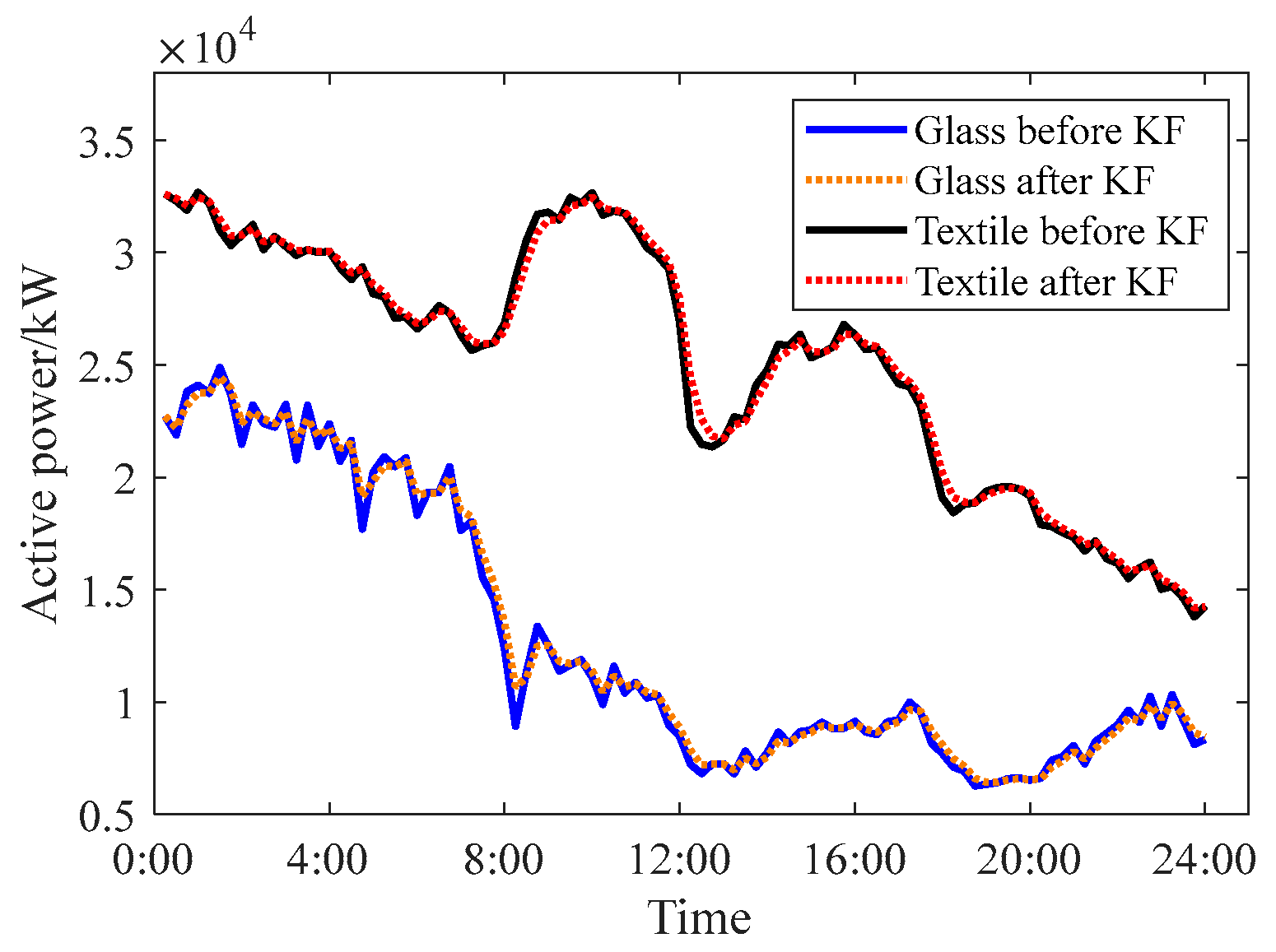
The original data underwent cleaning and noise reduction. Following the preprocessing of the original time series data, the KF was employed for noise removal. A comparison of load curves for textile and glass before and after filtering is depicted in Figure 6. The load curves, post-noise reduction, exhibit a smoother trajectory while preserving their essential characteristics. This establishes a foundation for the subsequent application of the K-means algorithm.
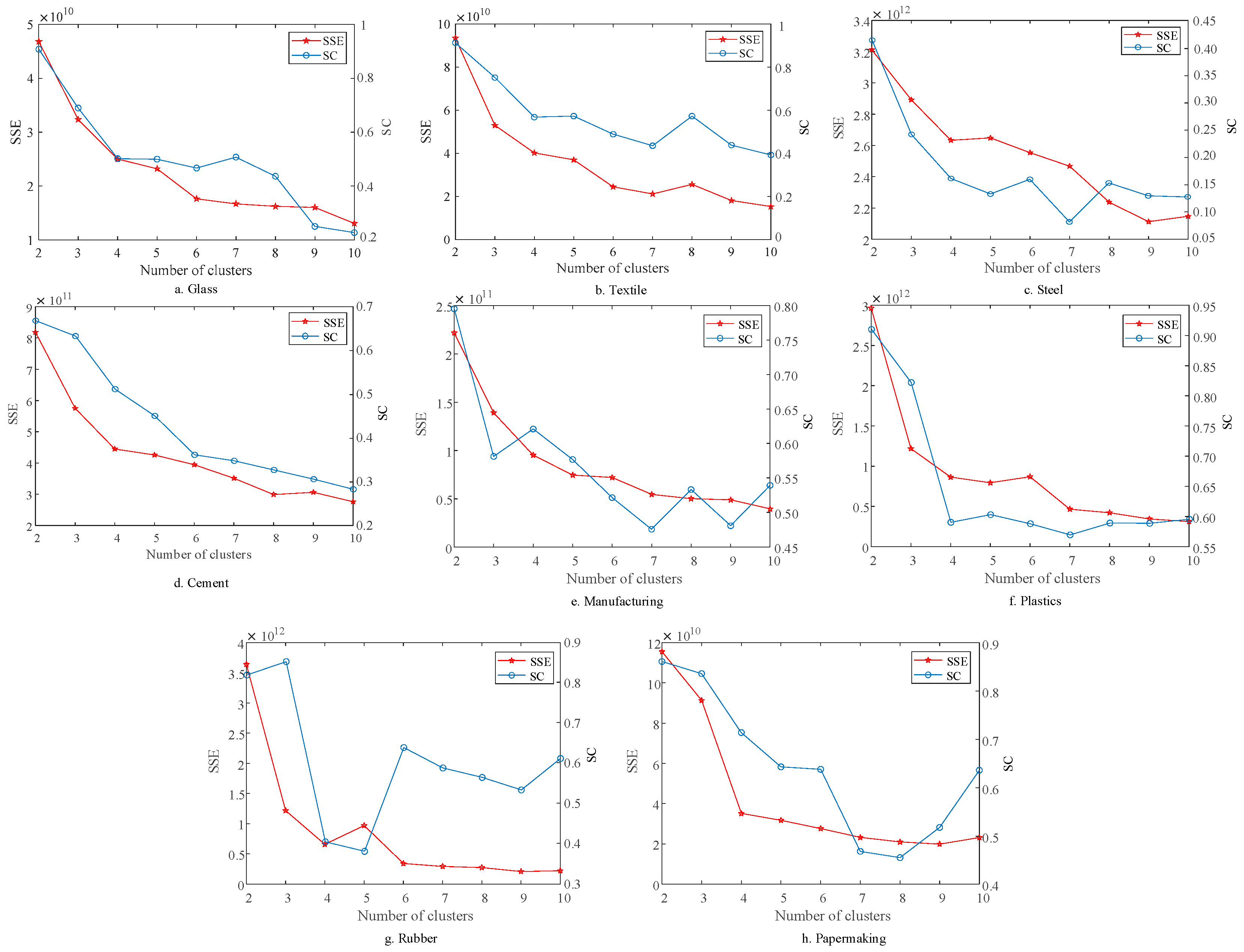
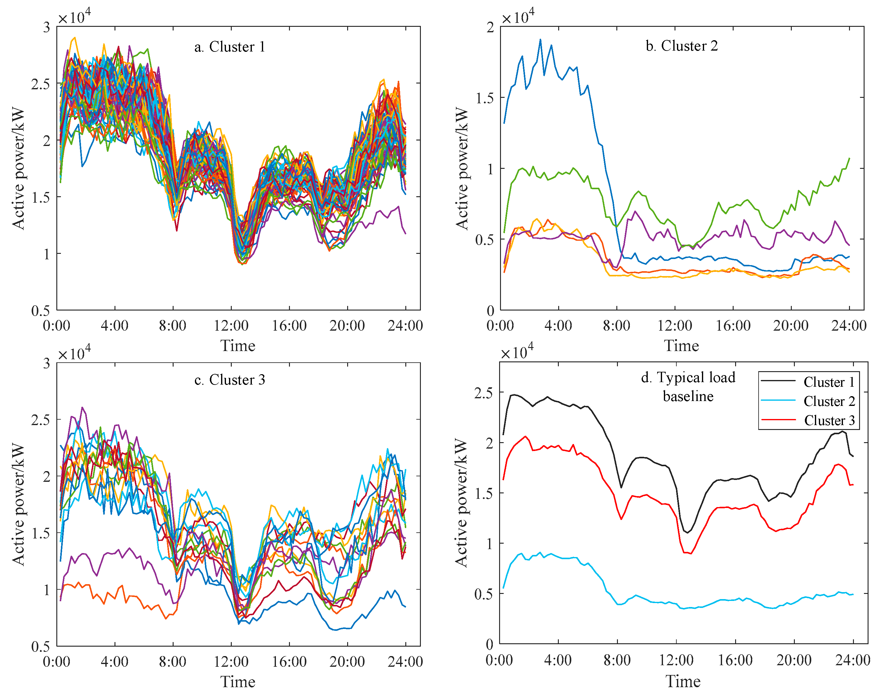
The SSE and SC for each industry are illustrated in Figure 7, with the SSE on the left half-axis representing the result obtained from the Elbow Method and the right half-axis showcasing the result obtained from the SC. According to the Elbow Method, the optimal number of clusters for papermaking is around four, and the optimal number of clusters (k = 3) is determined by integrating the SC. The optimal cluster numbers for glass, textile, steel, cement, manufacturing, plastics, and rubber are 3, 3, 3, 3, 4, 5, and 3, respectively. Specific cluster numbers k and total data numbers n for each industry are detailed in Table 4. Notably, the clustering effect of glass using the K-means algorithm is visualized in Figure 8. Figure 8 demonstrates that the K-means algorithm achieves a satisfactory clustering effect, with the distinct size and characteristics of the three types of load curves clearly evident. These three typical load baselines can be effectively utilized in subsequent strategy implementation.
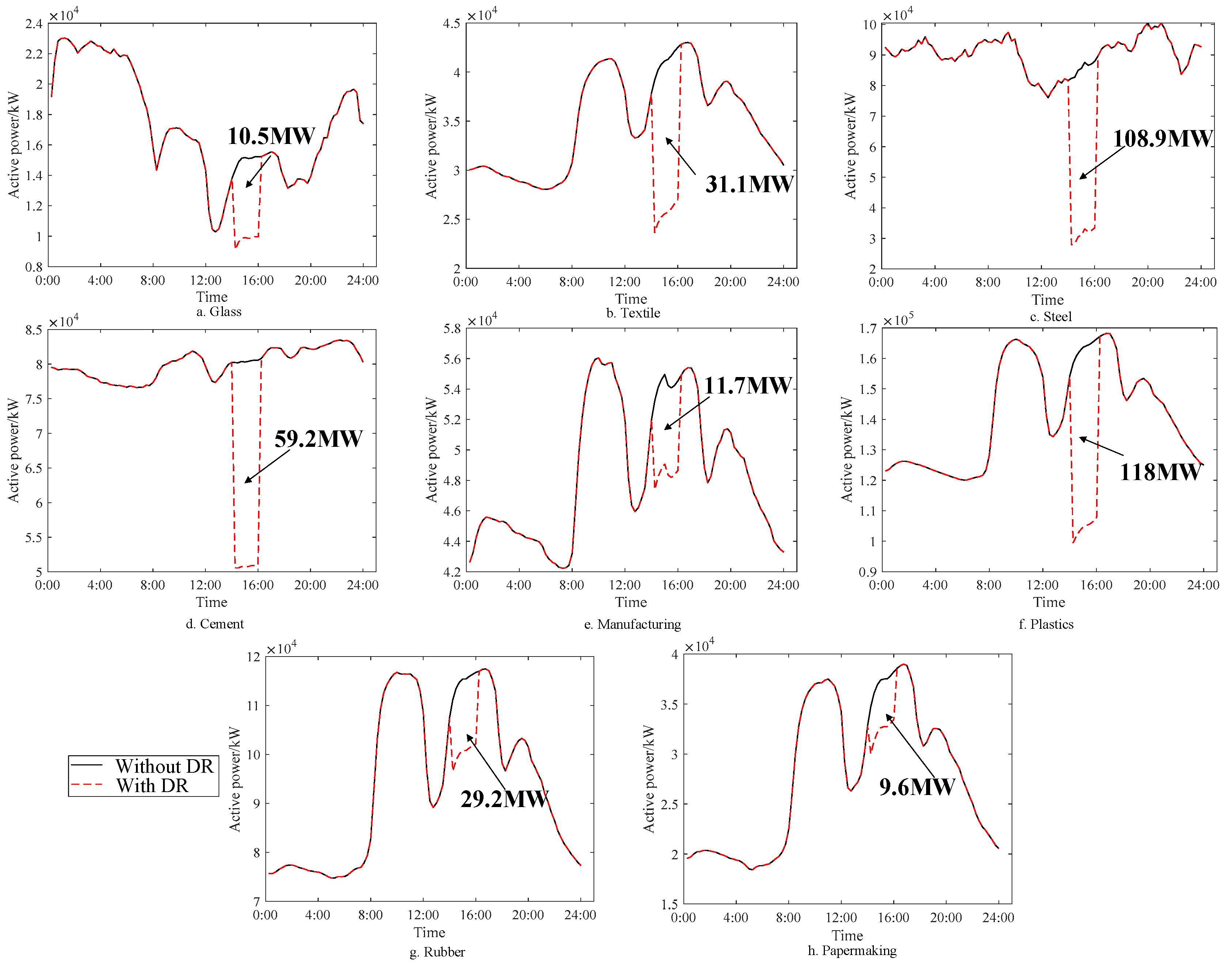
Assuming the DR time is 14:00–16:00 every day, the available DR potential is calculated based on the index proposed by the fuzzy control input. Table 5 displays the load flexibility of each industry, the baseline peak load rate of the typical load for each industry, and the user participation rate corresponding to the typical load baseline of each industry. Among them, steel has the highest response coefficient of approximately 0.6, followed by plastics, textiles, and cement. Meanwhile, the response factor for rubber, glass, papermaking, and manufacturing are roughly comparable. Figure 9 illustrates that among the eight industries, plastics exhibit the highest available DR potential, with an average of approximately 59 MW per hour, owing to their substantial electricity consumption and the highest proportion of flexible load, resulting in a high response factor. Despite steel production involving a lot of equipment and having the largest response factor, its available DR potential is the second highest at about 54.45 MW per hour as it does not have the highest electricity consumption. Due to their lower electricity consumption, papermaking and glass have the last two available DR potential values, averaging 4.8 MW and 5.25 MW per hour, respectively. The average hourly values for the remaining industries are approximately 15.6 MW for textile, 29.6 MW for cement, 5.85 MW for manufacturing, and 15.6 MW for rubber. Overall, the evaluation results align with the existing impressions and experiences of different industries.
The average available DR potential per hour across the eight industries is approximately 23.6 MW, with a total average available DR potential of around 189 MW. The maximum hourly load of the eight industries in the region is about 6.1 × 10² MW, and the available demand response potential accounts for about 31% of the maximum load.

7. Conclusions

In this study, a fuzzy control-based method for assessing DR potential is proposed to evaluate available DR potential, particularly in the early stages of DR implementation with limited data samples. The main conclusions of this paper are as follows: (1) an available DR potential evaluation framework with four steps is proposed; (2) the K-means clustering algorithm is used to effectively classify the load data of industrial users and obtain the typical baseline loads of different clustering scenarios; (3) a fuzzy control system is designed to predict the response factor, and three strongly correlated variables including electricity intensity, peak load rate and load flexibility are selected as the controller inputs; (4) the proposed fuzzy control evaluation method can assess the DR potential of different industrial users, providing valuable insights for power planning and dispatching departments in decision making.

Author Contributions

Conceptualization, Y.L.; Methodology, Z.L.; Formal analysis, N.D.; Resources, B.S.; Data curation, C.S.; Writing—original draft, B.L.; Writing—review & editing, J.R.; Visualization, Y.H. All authors have read and agreed to the published version of the manuscript.

Funding

This work is supported by the Novel Power System Technology Project of Guangdong Province (Project No. 1689819705078) and National Natural Science Foundation of China (Project No. U22B20114).

Data Availability Statement

The data presented in this study are available on request from the corresponding author. The data are not publicly available due to privacy.

Conflicts of Interest

Authors Yan Li, Zhiwen Liu, Chong Shao, Jiayu Rong, Nan Dong, Buyun Su and Yuejia Hong were employed by the company CSG. Author Bingjun Lin was employed by the company Beihai Power Supply Bureau Guangxi Power Grid Co., Ltd. They declare that the research was conducted in the absence of any commercial or financial relationships that could be construed as a potential conflict of interest.

References

  1. Tong, J.L.; Liu, W.S.; Mao, J.B.; Ying, M.L. Role and development of thermal power units in new power systems. IEEE J. Radio Freq. Identif. 2022, 6, 837–841. [Google Scholar] [CrossRef]
  2. Wang, S.Y.; Zhao, C.Y.; Fan, L.; Bo, R. Distributionally Robust Unit Commitment with Flexible Generation Resources Considering Renewable Energy Uncertainty. IEEE Trans. Power Syst. 2022, 37, 4179–4190. [Google Scholar] [CrossRef]
  3. Wang, B.; Li, Y.; Ming, W.Y.; Wang, S.R. Deep Reinforcement Learning Method for Demand Response Management of Interruptible Load. IEEE Trans. Smart Grid 2020, 11, 3146–3155. [Google Scholar] [CrossRef]
  4. U.S. Department of Energy. Benefits of Demand Response in Electricity Markets and Recommendations for Achieving Them; US Department of Energy: Washington, DC, USA, 2006.
  5. Emmanuel, B.; Chiu, M.C.; Hsu, H.W.; Lee, M.Y.; Wen, C.Y. Potential of Demand Response for Power Reallocation, a Literature Review. Energies 2022, 15, 863. [Google Scholar] [CrossRef]
  6. Wang, Z.; Lu, B.; Wang, B.; Qiu, Y.; Shi, H.; Zhang, B.; Li, J.; Li, H.; Zhao, W. Incentive based emergency demand response effectively reduces peak load during heatwave without harm to vulnerable groups. Nat. Commun. 2023, 14, 6202. [Google Scholar] [CrossRef] [PubMed]
  7. Pang, Y.; He, Y.; Jiao, J.; Cai, H. Power load demand response potential of secondary sectors in China: The case of western Inner Mongolia. Energy 2020, 192, 116669. [Google Scholar] [CrossRef]
  8. Faruqui, A.; Sergici, S. Household response to dynamic pricing of electricity: A survey of 15 experiments. J. Regul. Econ. 2010, 38, 193–225. [Google Scholar] [CrossRef]
  9. Daniel, T.; Wallin, F. Potential and barriers for demand response at household customers. Energy Procedia 2015, 75, 1189–1196. [Google Scholar]
  10. Mishra, M.K.; Murari, K.; Parida, S. Demand-side management and its impact on utility and consumers through a game theoretic approach. Int. J. Electr. Power Energy Syst. 2022, 140, 107995. [Google Scholar] [CrossRef]
  11. Zhou, F.Q.; Deng, L.C.; Wang, J.; Wang, H.Y.; Lu, F.; Chen, J.Q.; Wang, L.; Li, S.W.; Wang, J.F.; Jiang, X.M.; et al. Demand Side Resource Potential Analysis Methods and Application—Case Study on the City of Huzhou in the Yangtze River Delta; Natural Resources Defense Council: Beijing, China, 2020. (In Chinese) [Google Scholar]
  12. Strobel, N.; Fuhrländer-Völker, D.; Weigold, M.; Abele, E. Quantifying the Demand Response Potential of Inherent Energy Storages in Production Systems. Energies 2020, 13, 4161. [Google Scholar] [CrossRef]
  13. Jiang, Z.H.; Lee, Y.M. Deep transfer learning for thermal dynamics modeling in smart buildings. In Proceedings of the 2019 IEEE International Conference on Big Data (Big Data) 2019, Los Angeles, CA, USA, 9–12 December 2019; pp. 2033–2037. [Google Scholar]
  14. Kong, X.Y.; Kong, D.Q.; Yao, J.T.; Xiao, J. Online pricing of demand response based on long short-term memory and reinforcement learning. Appl. Energy 2020, 271, 114945. [Google Scholar] [CrossRef]
  15. Peirelinck, T.; Hermans, C.; Spiessens, F.; Deconinck, G. Domain randomization for demand response of an electric water heater. IEEE Trans. Smart Grid 2021, 12, 1370–1379. [Google Scholar] [CrossRef]
  16. Wohlfarth, K.; Klobasa, M.; Gutknecht, R. Demand response in the service sector-Theoretical, technical and practical potentials. Appl. Energy 2020, 258, 114089. [Google Scholar] [CrossRef]
  17. Kwon, P.S.; Østergaard, P. Assessment and evaluation of flexible demand in a Danish future energy scenario. Appl. Energy 2014, 134, 309–320. [Google Scholar] [CrossRef]
  18. Paulus, M.; Borggrefe, F. The potential of demand-side management in energy-intensive industries for electricity markets in Germany. Appl. Energy 2011, 88, 432–441. [Google Scholar] [CrossRef]
  19. Alkadi, N.; Starke, M.; Ma, O. Assessment of Industrial Load for Demand Response Across Western Interconnect; Oak Ridge National Lab.(ORNL): Oak Ridge, TN, USA, 2013.
  20. Jang, J.-S.R.; Sun, C.T. Neuro-fuzzy modeling and control. Proc. IEEE 1995, 83, 378–406. [Google Scholar] [CrossRef]
  21. Li, S.; Ahn, C.K.; Chadli, M.; Xiang, Z.R. Sampled-Data Adaptive Fuzzy Control of Switched Large-Scale Nonlinear Delay Systems. IEEE Trans. Fuzzy Syst. 2022, 30, 1014–1024. [Google Scholar] [CrossRef]
  22. Tong, S.C.; Min, X.; Li, Y.X. Observer-Based Adaptive Fuzzy Tracking Control for Strict-Feedback Nonlinear Systems with Unknown Control Gain Functions. IEEE Trans. Cybern. 2020, 50, 3903–3913. [Google Scholar] [CrossRef]
  23. Ding, S.H.; Zhang, B.B.; Mei, K.Q.; Park, J.H. Adaptive Fuzzy SOSM Controller Design with Output Constraints. IEEE Trans. Fuzzy Syst. 2022, 30, 2300–2311. [Google Scholar] [CrossRef]
  24. Huang, Y.L.; Zhang, Y.G.; Wu, Z.M.; Li, N.; Chambers, J. A Novel Adaptive Kalman Filter with Inaccurate Process and Measurement Noise Covariance Matrices. IEEE Trans. Autom. Control 2018, 63, 594–601. [Google Scholar] [CrossRef]
  25. Jeon, J.Y.; Choi, J.S.; Byun, H.G. Implementation of elbow method to improve the gases classification performance based on the RBFN-NSG algorithm. J. Sens. Sci. Technol. 2016, 25, 431–434. [Google Scholar] [CrossRef]
  26. Zhou, H.B.; Gao, J.T. Automatic method for determining cluster number based on silhouette coefficient. Adv. Mater. Res. 2014, 3244, 227–230. [Google Scholar] [CrossRef]
  27. Zhou, S.; Xu, Z.; Liu, F. Method for Determining the Optimal Number of Clusters Based on Agglomerative Hierarchical Clustering. IEEE Trans. Neural Netw. Learn. Syst. 2017, 28, 3007–3017. [Google Scholar] [CrossRef] [PubMed]
  28. Peoples Government of Guangdong Province. Guangdong Statistical Yearbook; People’s Government of Guangdong Province: Guangzhou, China, 2022. (In Chinese)
  29. Cheng, Y.; Rao, R.; Ding, S. Potential analysis of power demand side adjustable load in industrial field. Energy Eng. 2023, 43, 72–78. (In Chinese) [Google Scholar]
  30. Feng, J.; Zhou, Y.F. The analysis of typical load characteristic and the ability of interruptible load of the electrical customer in Zhejiang province. Power Demand Side Manag. 2011, 13, 48–53. (In Chinese) [Google Scholar]
  31. Anand, A.; George, V.; Kanthi, R.; Tagore, M.; Padmashree, M. Basics on Categorizing Travel-Time-Based Degrees of Satisfaction Using Triangular Fuzzy-Membership Functions. Transp. Res. Procedia 2020, 48, 1555–1574. [Google Scholar] [CrossRef]
  32. Kompil, M.; Celik, H. Modelling trip distribution with fiuzzy and genetic fuzzy systems. Transp. Plan. Technol. 2013, 36, 170–200. [Google Scholar] [CrossRef]
  33. Kedia, A.; Saw, K.; Kati, B.K. Fuzzy Logic Approach in Mode Choice Modelling For Education Trips: A Case Study of Indian Metropolitan City. Transport 2015, 30, 286–293. [Google Scholar] [CrossRef]
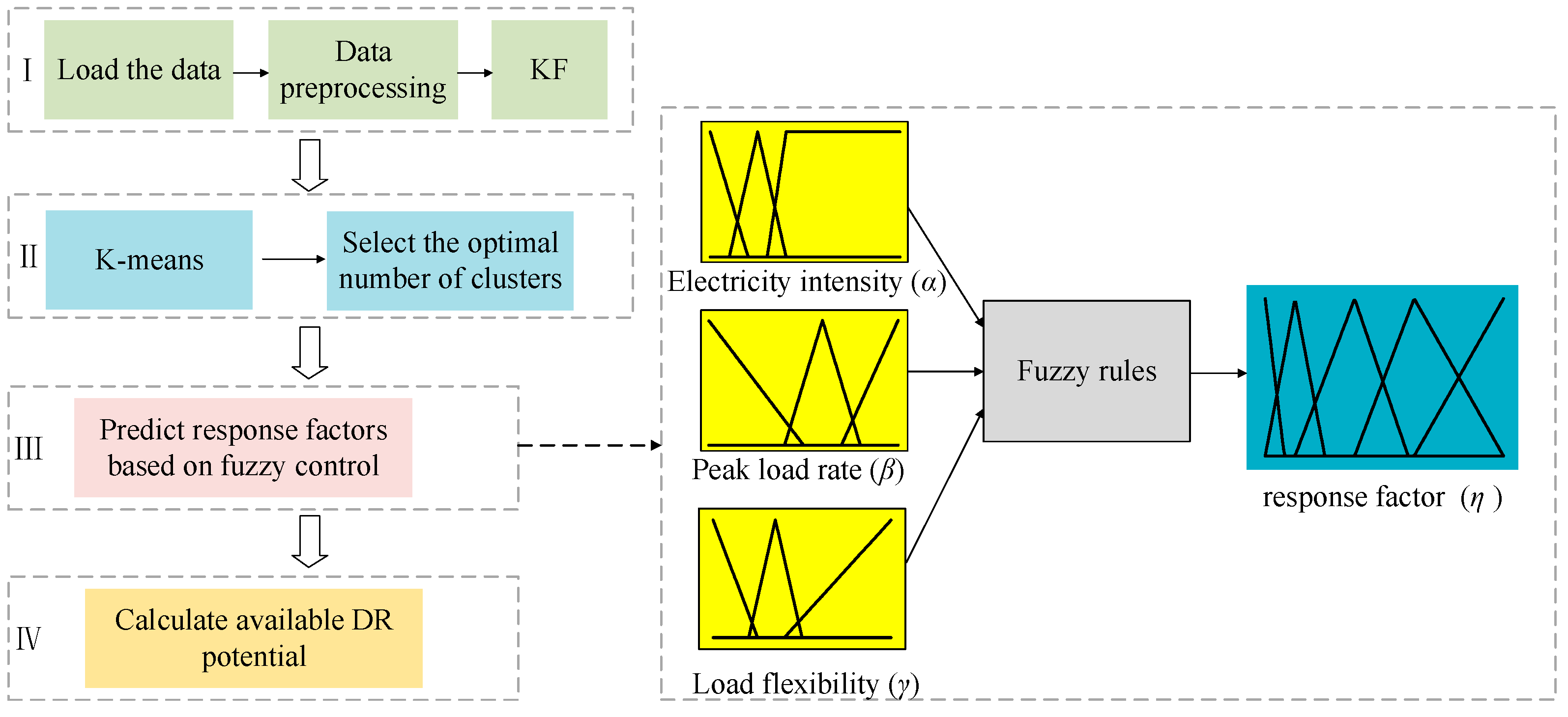
Figure 1. Available DR potential evaluation framework based on fuzzy control.
Energies 17 05146 g001
Figure 2. Flow chart of selection of optimal cluster number.
Energies 17 05146 g002
Figure 3. The electricity intensity of typical industry types in China.
Energies 17 05146 g003
Figure 4. Evaluation process of load flexibility.
Energies 17 05146 g004
Figure 5. The processes of predicting response factor.
Energies 17 05146 g005
Figure 6. Comparison of load before and after KF.
Energies 17 05146 g006
Figure 7. Graphs of SSE and SC for each industry.
Energies 17 05146 g007
Figure 8. Clustering result of glass.
Energies 17 05146 g008
Figure 9. Comparison of industrial load with and without DR.
Energies 17 05146 g009
Table 1. Key variables.
Subscript iIndustrial User iλijthe Weight of Cluster j
subscript jj-th clusterαielectricity intensity
fi(t)load dataset of industrial user iρiGDP of industrial user i
kclustering numberζiannual electricity consumption
Pijj-th typical load baseline of user iβijpeak load rate of cluster j
mitotal sample number γiload flexibility of industrial user i
nijdata number of the cluster jηijresponse factor of cluster j
Table 2. Flexible load ratio in typical industries.
Industrial TypeMain Regulating EquipmentFlexible Load Ratio
Glassglass melter; annealing furnace; air compressor; glass cutting machine; belt conveyor; toughening furnace25%
Textiletexturing machine; double-twisting machine; can tipper; loom machine; workshop lighting35%
Steelelectric furnace; bloomery; oxygenerator; steel rolling production line; bar production line; wire production line20%
Cementrotary kiln; shaft kiln; raw mill; cement grinding mill; ball mill; air compressor; conveyor tape machine24%
Manufacturingfurnace for heat treatment; high-frequency furnace; melting furnace; blower; dryer; cooling pump; vetilator20%
Plasticselectric heaters; box mill; ultrasonic equipment; eyelet machine; wire press machine; high-velocity ram machine64%
Rubberlinard machine; motorshipengine; edger; conveyor; water washer33%
Papermakingreeling machine; crane8%
Table 3. Fuzzy rule table.
L3M3S3
L2M2S2L2M2S2L2M2S2
S1VLVLLLMMSSVS
M1LLMMMSSVSVS
L1MSSMSSVSVSVS
Table 4. Cluster details of 8 industries.
Industrial TypeClustering Results
kn
Glassk = 3n = [71, 5, 15]
Textilek = 3n = [5, 67, 19]
Steelk = 3n = [26, 34, 34]
Cementk = 3n = [40, 43, 8]
Manufacturingk = 4n = [25, 5, 47, 14]
Plasticsk = 5n = [38, 4, 12, 3, 34]
Rubberk = 3n = [74, 1, 16]
Papermakingk = 3n = [71, 4, 16]
Table 5. Peak load rate, load flexibility, and response factor of each industry.
Industrial TypePeak Load RateLoad FlexibilityResponse Factor
Glassγ1 = 0.663, γ2 = 0.481, γ3 = 0.6592.57 η1 = η3 = 0.348, η2 = 0.125
Textileγ1 = 0.971, γ2 = 0.988, γ3 = 0.9913.03η1 = η2 = η3 = 0.366
Steelγ1 = 0.731, γ2 = 0.937, γ3 = 0.8333.1η1 = η3 = 0.609, η2 = 0.611
Cementγ1 = 0.966, γ2 = 0.967, γ3 = 0.8653.21η1 = η2 = 0.366, η3 = 0.365
Manufacturingγ1 = 0.98, γ2 = 0.928, γ3 = 0.98, γ4 = 0.9632.15η1 = η2 = η3 = η4 = 0.11
Plasticsγ1 = 0.991, γ2 = 0.849, γ3 = 0.961, γ4 = 0.982, γ5 = 0.9853.13η1 = η2 = η3 = η4 = η5 = 0.463
Rubberγ1 = 0.995, γ2 = 1, γ3 = 0.9761.85η1 = η2 = η3 = 0.125
Papermakingγ1 = 0.98, γ2 = 0.97, γ3 = 0.9831.57η1 = η2 = η3 = 0.125
Disclaimer/Publisher’s Note: The statements, opinions and data contained in all publications are solely those of the individual author(s) and contributor(s) and not of MDPI and/or the editor(s). MDPI and/or the editor(s) disclaim responsibility for any injury to people or property resulting from any ideas, methods, instructions or products referred to in the content.