A Comparative Analysis of Machine Learning Techniques for Predicting the Performance of Microchannel Gas Coolers in CO₂ Automotive Air-Conditioning Systems

Abstract

The automotive industry is increasingly focused on developing more energy-efficient and eco-friendly air-conditioning systems. In this context, CO₂ microchannel gas coolers (MCGCs) have emerged as promising alternatives due to their low global warming potential (GWP) and environmental benefits. This paper explores the application of machine learning (ML) algorithms to predict the thermohydraulic performance of MCGCs in automotive air-conditioning systems. Using data generated from an experimentally validated numerical model, this study compares various ML techniques, including both linear and nonlinear regression models, to forecast key performance metrics such as refrigerant outlet temperature, pressure drop, and heat transfer rate. Spearman’s correlation was employed to develop performance maps, whereas the R² and MSE metrics were used to evaluate the models’ predictive accuracy. The linear models gave around 70% forecasting accuracy for pressure drop across the gas cooler and 97% accuracy for refrigerant outlet temperature, whereas the nonlinear models achieved more accurate predictions, with an accuracy ranging from 71% to 99%. This implies that nonlinear regression generally performs better than linear regression models in assessing the overall thermohydraulic performance of microchannel gas coolers. This research brings forth new ideas on how ML methods can be applied to enhance efficiency and effectiveness in gas coolers, contributing to the development of more eco-friendly automotive air-conditioning systems.

1. Introduction

The need for compact, effective heat exchangers has emerged due to various reasons, such as increased demands for energy, space limitations in device packaging, and the necessity to save resources and energy. Heat transfer intensification has increasingly become a research interest for scientists over the past two decades [1]. Over time, there has been much emphasis on small flow passages known as microchannels in refrigeration, air-conditioning, and power generation applications. Microchannels have been defined by Mehendale et al. [2] as channels having dimensions ranging from 1 µm to 100 µm. One of the most typical uses of MCHXs is in MAC systems, where they work as gas coolers, transferring heat from the refrigerant to ambient air.

The MACs in electric cars find gas coolers very useful. They take away the heat from the refrigerant and let it out into the air around the car [3]. An expansion valve allows high-pressure refrigerant gas to enter after having left the compressor. In this process, a refrigerant passes through an evaporator, which makes it cool and expand, causing vehicle air to cool down too [4]. The use of refrigerants in MACs presents a problem because there has been an increase in bans on using gasses with a high warming potential (GWP) due to the Kigali amendment, their continuous increase, and the environmental damages that occur as a result [5,6]. Nontoxic nonflammable microchannel carbon dioxide (CO₂) gas coolers have practically no GWP and are environmentally friendly (“Amendment to the Montreal Protocol on Substances That Deplete the Ozone Layer,” 2016) [7]. These may be regarded as promising alternatives to traditional refrigerants, and they will have a significant role in the near future of MACs.

Numerical models primarily rely on mathematical equations and algorithms to represent the relationships between variables. These models consider intricate details of the system being modeled, such as geometric details, the materials used, and the working fluid [8,9,10,11,12,13]. They provide insight into the underlying mechanisms that govern a system’s behavior. However, they require a detailed understanding of the system and can be complex and time-consuming to construct. In contrast, machine learning (ML) models have recently emerged as a promising alternative; they do not rely on physical principles and are based solely on empirical data. ML algorithms are computationally more economical than numerical simulations, and they allow for a more rapid simulation. Furthermore, ML algorithms are more flexible than numerical simulations, and they can predict performance under a wider range of operating conditions and geometric configurations.

Conventional curve-fitting techniques are suitable for datasets that have a limited number of input variables and a small sample size. But, when datasets involve many input variables and complex inter-relationships among them, more advanced algorithms are required. Many researchers have recently ventured into investigating the application of ML algorithms in different areas, including cyber security, social media, manufacturing, and even self-driving cars. Some researchers are also involved in integrating ML techniques into heat transfer, pressure drop, and fluid mechanics. The idea is to take care of existing complications within these subjects [14,15,16,17,18,19]. Ma et al. [18] employed numerical simulations and parameter sensitivity analysis, which involved a gradient-boosting tree machine learning model, to find major factors affecting fluid flow and heat transfer in rectangular microchannels. Their results indicated that, under low-Reynolds-number conditions, the number of channels and the Reynolds number significantly influence the heat transfer performance, but the cross-sectional area and aspect ratio have a great impact on the pumping power. Arman et al. [20] used a committee neural network (CNN) to predict the pressure drop in microchannels under various conditions. Their modeling approach used 329 empirical data points to establish the relationship between the pressure drop and factors such as fluid properties, the hydraulic diameter of the channel, and vapor quality. To determine the weight coefficients for each network in the CNN, a genetic algorithm was used. The findings of their study revealed that combining all algorithms via a weighted averaging method yielded the most favorable value for the average absolute relative deviation (AARD%) at 5.79. This investigation demonstrates that the precision of CNN predictions improves when multiple techniques are integrated and highlights the potential of a CNN for accurate predictions across different fields. Matthew T. Hughes et al. [21] developed a comprehensive model for predicting the heat transfer coefficient and frictional pressure drop in horizontal MCHXs. Their model was built using a dataset that comprised over 4000 data points and covered the entire range of vapor quality. Their dataset encompassed various mass fluxes (50–800 kg m⁻² s⁻¹), low pressures (0.03–0.96), and hydraulic diameters (0.1–14.45 mm). The authors compared various models, including flow-regime-based correlations and ML regression models. Remarkably, they found that ML algorithms—the random forest model in particular—provided the best prediction performance for both pressure drop and heat transfer and achieved an average absolute deviation of approximately 4% for both. Kim et al. [22] developed universal machine learning models to predict the thermal performance of micro pin-fin heat sinks across various shapes and operating conditions. To achieve this, they used power law regression and a comprehensive database containing 906 data points from 15 different studies. The evaluation of the ML models demonstrated mean absolute error values that ranged from 7.5% to 10.9%. These results signify a substantial enhancement in prediction accuracy and are approximately five times better than existing regression correlations. Recently, Yu [23] performed numerical simulations to investigate the flow and heat transfer phenomena within an elliptical pin-fin microchannel heat sink. They then used artificial neural networks to predict key parameters such as the average temperature, temperature non-uniformity, and pressure drop within the microchannel.

This study attempts to resolve the uncertainties surrounding ML models in MCGCs, an area that has not been explored. To achieve this, we conducted a study employing an explainable ML approach to elucidate the black box of the ML model. Our primary objective was to gain comprehensive insight into the predictions of multiple ML models and understand the effect of geometric and operational parameters on MCGC performance. Our methodology involved using an experimentally validated numerical model [24,25] to generate a substantial dataset of 13,000 data points for the training of the ML models, which minimized the need for traditional experimentation and thereby reduced computational time and material resources. We used Spearman’s correlation for the generation of performance maps, enabling a deeper understanding of the ML models. Through this interpretation, we delineated the effects of the input parameters on the performance variables to plot the correlations among them. This visualization will assist researchers in pinpointing optimal design variables for the efficient development of MCGCs. Furthermore, rather than relying on a single ML model, we employed eight representative models derived from linear and nonlinear regression algorithms.

2. Methods

Figure 1 illustrates a flowchart of the procedure adopted in this study to evaluate the performance of an MCGC, outlining a systematic methodology comprising several key steps. First, relevant data on the performance of the MCGC—including various geometric parameters and operating conditions—were gathered and organized into a dataset. These raw data were then preprocessed, which involved addressing missing values and normalizing and standardizing numerical features. Next, a detailed analysis of the dataset was conducted using statistical methods and visualization techniques to comprehend the data distributions and identify data patterns. Feature selection techniques were employed to identify the most important variables influencing performance, following which model parameters were tuned for optimal results. The ML models were trained using the preprocessed data, which were split into training (80%) and testing (20%) sets. Following model training, key performance parameters, such as the heat transfer rate (Q), pressure drop (ΔP), outlet temperature of the refrigerant (T_ro), and outlet temperature of air (T_ao), were predicted using the test data. The performance of each model was then assessed using metrics such as the mean squared error (MSE) and the coefficient of determination (R²), enabling a direct comparison to identify the best-performing model. This methodology ensured thorough data preparation, accurate model training, and the selection of the most effective model for predicting the performance of the MCGC.

2.1. Dataset

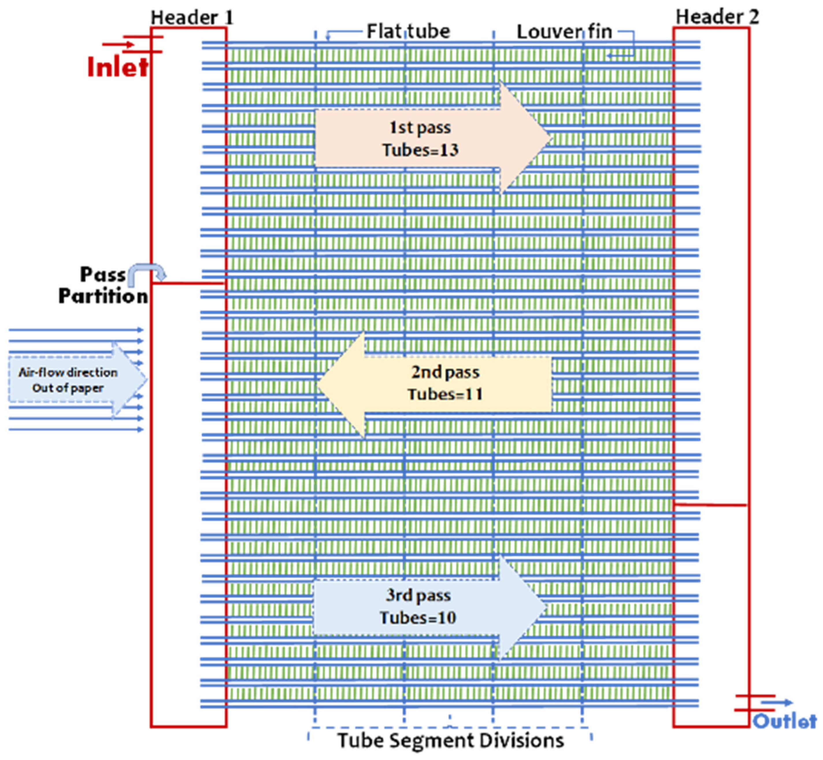
The dataset utilized in this study was derived from the MCGC database used in previous research [24], as illustrated in Figure 2. To train the ML models, data generated by an experimentally validated numerical model were utilized. Approximately 13,000 datasets were extracted, encompassing 23 input parameters and four output parameters that served as performance indicators.

The dataset captured a broad spectrum of geometric conditions, including variations in the number of passes, tubes, and ports, as well as tube pitch, fin pitch, and fin height. Furthermore, the MCGC was subjected to diverse operating conditions during the simulations, with ambient temperatures ranging from 42 to 56 °C, inlet air flow rates ranging from 0.45 to 0.70 kg/s, refrigerant flow rates varying from 0.018 to 0.057 kg/s, and refrigerant inlet temperatures spanning 106 to 148 °C. This wide range of geometric and operating conditions enabled an in-depth analysis of the MCGC’s performance under diverse scenarios.

2.2. Data Preprocessing and Feature Selection

The dataset, which included the geometric and operating conditions of the selected MCGC, was meticulously checked for missing, constant, and duplicate values. Thereafter, preprocessing steps were implemented to address any identified issues, ensuring the dataset’s integrity and readiness for subsequent analysis. To ensure the integrity of our regression analysis, we implemented a rigorous approach to outlier removal. Specifically, the interquartile range (IQR) method was adopted to detect outliers, identifying any data points that fell below the first quartile or above the third quartile by more than 1.5 times the IQR. Notably, this method is widely known for its ability to detect extreme values without making assumptions regarding the data distribution. Furthermore, we visually inspected the box plots for each feature, aiming to validate that the detected outliers were indeed genuine irregularities rather than critical data points. This approach ensured that all outliers in the dataset were addressed while minimizing the risk of eliminating meaningful data. The impact of outlier removal was assessed by comparing model performance with and without these extreme values. The results revealed that excluding outliers enhanced model stability and improved predictive accuracy without introducing any bias into the results.

Our models were implemented in Python, utilizing various open-source libraries to facilitate analysis. Specifically, we employed pandas for loading and manipulating the data in a tabular format, NumPy for performing mathematical operations, and matplotlib for creating visualizations. Furthermore, we used sklearn.linear_model for implementing different regression models, sklearn.preprocessing for transforming the data before regression, sklearn.model_selection for splitting the data into training and test sets and performing cross-validation, and sklearn.metrics for evaluating the performance of the ML models using the selected metrics.

Notably, various correlation coefficients can be employed to quantify the relationship between different parameters or variables. Among the most commonly used correlation coefficients are the Pearson correlation coefficient, Spearman’s rank correlation coefficient, and Kendall’s rank correlation coefficient. Each of these coefficients offers distinct methods for quantifying the relationships between variables, depending on the nature of the chosen data. Hence, selecting the correlation coefficient that is most appropriate for the types of variables involved in the analysis is critical. Given that both linear and nonlinear relationships were observed between the input and output parameters of this study, Spearman’s rank correlation coefficient was preferred over the others. Alongside this Spearman’s correlation analysis, we also performed a variance inflation factor (VIF) analysis to detect any multicollinearity among the independent predictors. Notably, the VIF analysis quantifies the extent to which the variance of a regression coefficient is inflated owing to its correlation with other predictors in the model [26]. Typically, VIF values above 5 indicate problematic levels of multicollinearity that can distort the regression results. Fortunately, in our analysis, none of the predictors demonstrated a VIF value exceeding 5. The VIF values for the selected features ranged from 1.174 (for the number of passes) to 4.380 (for the mass flow rate of air, ṁ_a), as indicated in

Table 1. Variance inflation factor (VIF) values for the selected features.

Feature	VIF
Tri	4.148168
Pri	3.455498
Tai	2.7185492
ṁr	2.576147
ṁa	4.380292
Tube length	3.798371
No. of tubes	3.892001
No. of ports	1.218008
No. of passes	1.174228

. Notably, the highest VIF values were recorded for ṁ_a (4.38) and the number of tubes (3.89), indicating moderate multicollinearity. However, these values lie well below the threshold for concern, prompting us to conclude that the observed multicollinearity is not significant enough to necessitate the exclusion of any variables. This step ensures that all selected predictors can be utilized in the models without compromising their accuracy or interpretability.

Generally, to evaluate the performance of a model, data are split into two sets: a training set and a testing set. The training set is used to train the model, allowing it to learn the relationships between the input features and output values. The testing set, on the other hand, is used to evaluate the model’s performance on unseen data, thereby assessing its ability to generalize its predictions to new data points. In this study, the size of the test set was set to 0.2, implying that 20% of the data were allocated for testing, while the remaining 80% were designated for training. Furthermore, the random state parameter was set to 1 to ensure the reproducibility of the split. The resulting training set (X_train and y_train) was used to train different ML models, while the testing set (X_test and y_test) was utilized to evaluate their performance.

2.3. Model Development and Evaluation

In this study, we selected eight representative ML models to predict the thermohydraulic performance of the selected MCGC. These models were drawn from two primary categories: linear-regression-based models and nonlinear-regression-based models. Our objective was to identify the most suitable model for predicting the dependent output parameters—heat transfer rate, air temperature, refrigerant temperature, and pressure drop—based on the provided input geometric parameters and operating conditions. A detailed description of these ML models is provided below.

Linear-regression-based ML models are parametric and supervised learning algorithms that predict outcomes by assuming a linear relationship between the input and output variables. For our analysis, four models were selected from this category: linear regression, ridge regression, lasso regression, and elastic net. Notably, for ridge and lasso regression, the regularization parameter (λ) is a crucial hyperparameter that controls the extent of shrinkage applied to the coefficients, aiding in the mitigation of overfitting. To determine the optimal value of λ, we employed a Bayesian search technique using cross-validation (BayesSearchCV), following the approach adopted by Ullah et al. [27]. This process involved five-fold cross-validation over a range of possible λ values, identifying the λ value that minimized the cross-validation error. The search was conducted over 20 iterations with a fixed random state to ensure reproducibility. In cases where specific search parameters for regularization were not available, the models were trained under default settings.

Nonlinear-regression-based ML models extend the principles of linear regression to capture more intricate relationships between input and output variables. In this study, four models from this category were examined: polynomial regression, the generalized additive model (GAM), the long short-term memory (LSTM) network, and Weibull regression. By comparing these models, we aimed to determine the most effective framework for accurately predicting the thermohydraulic performance of the MCGC under various geometric and operating conditions.

To quantify the accuracy of the ML models, two error metrics were employed: MSE and R². The MSE is particularly useful because it allocates greater weight to larger errors, making it a highly sensitive measure of performance. Meanwhile, the R² score assesses the predictability of an ML model by determining the proportion of variance in the dependent variable that is explained by the independent variables. Typically, a well-performing ML model should exhibit an R² score close to 1.

3. Results and Discussion

3.1. Feature Selection and Model Training

To enhance the efficiency and accuracy of the predictive models, feature selection was performed on the preprocessed dataset. This involved using statistical techniques and correlation analysis to identify the most significant variables influencing the target variable. By reducing the number of features from an initial count of 27 to a more manageable count of 13, the complexity of the models was alleviated, thereby minimizing the risk of overfitting and enhancing the generalizability of the models.

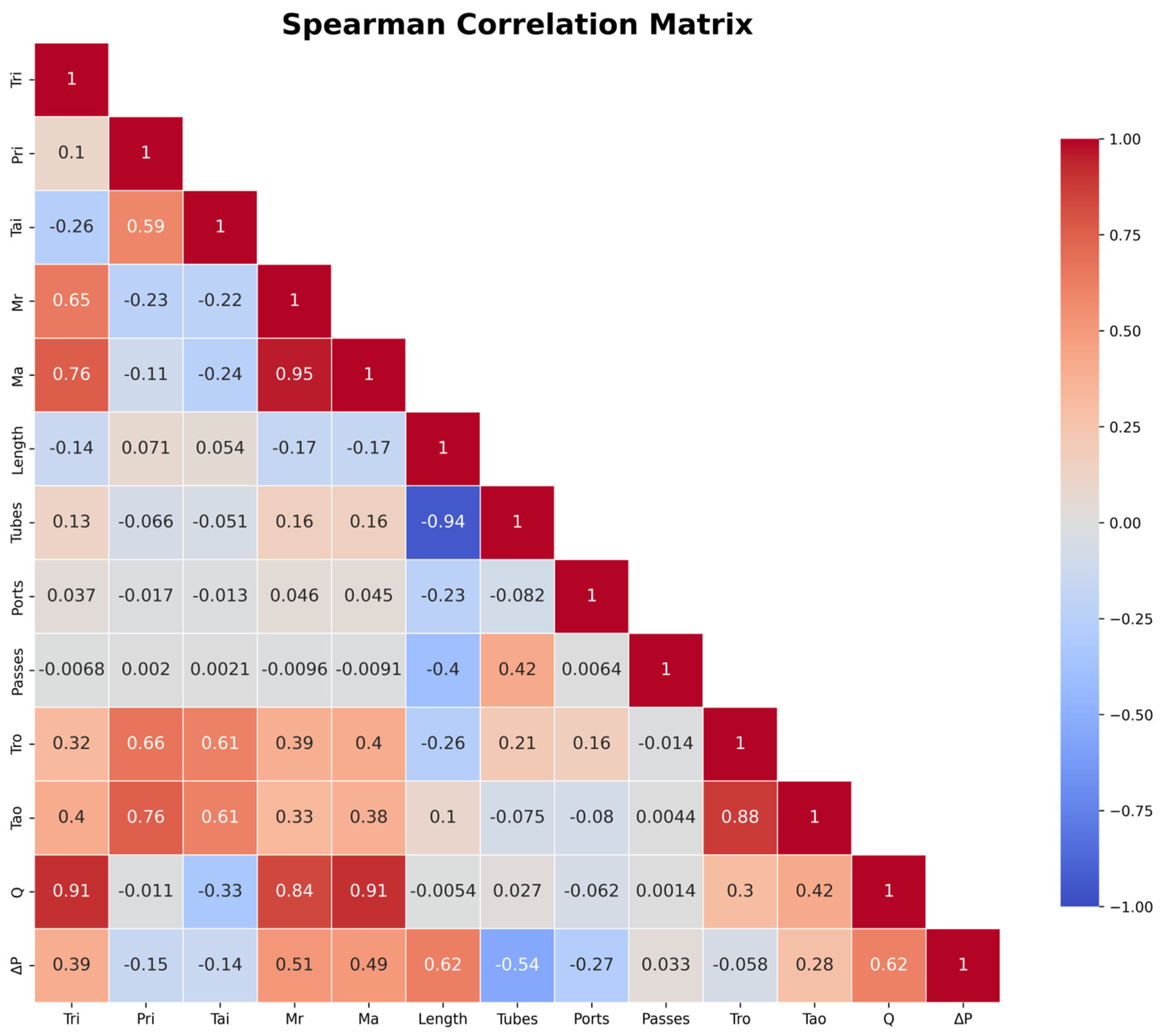
Figure 3 presents a Spearman correlation matrix illustrating the strength and direction of the relationships between the variables in the dataset. Notably, the values of the correlation coefficient range from −1 to +1, where +1 indicates a perfect positive relationship—implying that as one variable increases, the other also increases. Meanwhile, a coefficient value of −1 signifies a perfect negative relationship, where one variable increases as the other decreases. Finally, a coefficient value close to zero suggests no strong linear correlation between the concerned variables.

The heatmap indicates that certain variables exhibit strong correlations with one another. For instance, the operating parameters ṁ_a and mass flow rate of refrigerant (ṁ_r) display a high positive correlation coefficient of 0.95, indicating a robust relationship where changes in ṁ_a are closely linked to changes in ṁ_r. This suggests that both parameters are key factors influencing the system’s performance, particularly in terms of the gas cooler capacity (denoted as Q), which exhibits positive correlations with both ṁ_a (0.88) and ṁ_r (0.61).

In contrast, geometric parameters such as the length of tubes and the number of tubes, ports, and passes exhibit substantially weaker correlations with gas cooler capacity. For instance, the length of tubes and number of tubes exhibit near-zero correlations with Q (0.16 and 0.046, respectively), indicating their minimal impact on gas cooler capacity. However, geometric parameters such as the number of tubes (−0.54) and tube length (−0.52) display moderate negative correlations with pressure drop (ΔP), underscoring their significance in predicting pressure-related behaviors within the system.

Notably, operating conditions such as inlet refrigerant temperature (T_ri) and inlet refrigerant pressure (P_ri) display weak correlations with ΔP (−0.15 and −0.19, respectively), further reinforcing the notion that geometric parameters have a more significant impact on ΔP. Interpretations of these correlation coefficients indicate that operating parameters such as ṁ_a, ṁ_r, and T_ri substantially influence gas cooler capacity, while geometric parameters exert more pronounced impacts on pressure drop. Based on this analysis, we selected nine critical input variables—ṁ_a; T_ai; ṁ_r; P_ri; T_ri; heat exchanger length; number of tubes, ports, and passes—to train the ML algorithms. Notably, these variables capture the essential relationships identified in the correlation matrix, ensuring that the ML models are informed by the most relevant features for predicting both gas cooler capacity and pressure drop. Furthermore, the VIF analysis confirmed that no predictor had a VIF value exceeding 5, with the highest VIF values observed for ṁ_a (4.38) and the number of tubes (3.89), indicating moderate but non-problematic collinearity. Consequently, we retained all predictors for the final models.

Both linear- and nonlinear-regression-based models were trained on the selected features. The linear-regression-based models were employed to capture the straightforward, proportional relationships between the variables, while the nonlinear-regression-based models were intended to uncover more complex patterns within the data. The training process involved optimizing model parameters to minimize prediction errors, thereby ensuring that the models could effectively predict the target variable under diverse conditions.

3.2. Performance Metrics

As stated previously, the MSE and R² metrics were used to evaluate the accuracy of the ML model predictions. The MSE represents the average squared difference between predicted and actual values and can be calculated using Equation (1):

$$\mathrm{M}\mathrm{S}\mathrm{E}={\displaystyle \frac{1}{\mathrm{n}}}\sum {\left({\mathrm{y}}_{\mathrm{i}}-\widehat{{\mathrm{y}}_{\mathrm{i}}}\right)}^2,$$

(1)

where n denotes the number of samples in the dataset, y_i represents the actual value of the i-th sample, and ŷ_i denotes the predicted value of the i-th sample. Meanwhile, the R² score, which quantifies the predictability of the ML model, can be expressed mathematically as in Equation (2):

$${\mathrm{R}}^2=1-{\displaystyle \frac{\sum {\left({\mathrm{y}}_{\mathrm{i}}-\widehat{{\mathrm{y}}_{\mathrm{i}}}\right)}^2}{\sum {\left({\mathrm{y}}_{\mathrm{i}}-\overline{\mathrm{y}}\right)}^2}}$$

(2)

where yᵢ denotes the actual value, ŷ_i represents the predicted value, and ȳ denotes the mean of the actual values.

The R² and MSE values for the regression models, including four linear models (linear, ridge, lasso, and elastic net) and four nonlinear models (polynomial, GAM, LSTM, Weibull), utilized in this study are summarized in

Table 2. Statistical metrics for the proposed machine learning (ML) models.

	Q (kW)		∆P (MPa)		Tro (°C)		Tao (°C)
	R2	MSE (×10−2 (kW)2)	R2	MSE (×10−2 (MPa)2)	R2	MSE (°C)2	R2	MSE (°C)2
Linear regression	0.99	2.95	0.71	0.452	0.97	0.545	0.99	0.057
Ridge regression	0.99	2.95	0.71	0.451	0.97	0.545	0.99	0.057
Lasso regression	0.98	3.69	0.70	0.460	0.96	0.861	0.98	0.191
Elastic net	0.98	3.43	0.71	0.451	0.96	0.857	0.98	0.187
Polynomial regression	0.99	3.43	0.96	0.052	0.99	0.142	0.99	0.013
Generalized additive model	0.99	0.78	0.71	0.460	0.99	0.038	0.99	0.005
Long short-term memory	0.99	0.53	0.99	0.01	0.99	0.108	0.99	0.022
Weibull regression	0.99	0.49	0.72	0.450	0.99	0.140	0.99	0.022

. This evaluation focuses on four key output parameters: gas cooler capacity, pressure drop, refrigerant outlet temperature, and air outlet temperature. Notably, all models accurately predict gas cooler capacity and air outlet temperature, achieving impressive accuracy rates exceeding 99%. In contrast, the pressure drop prediction accuracies of all linear-regression-based models are approximately 70%. In comparison, the nonlinear-regression-based models, namely polynomial, GAM, LSTM, and Weibull, achieve notably higher accuracies of 96%, 71%, 99%, and 72%, respectively. A similar trend is observed in the R² values associated with refrigerant outlet temperature, where the linear models score approximately 97%, while their nonlinear counterparts achieve accuracies exceeding 99%.

Table 2 also outlines the MSE values for the abovementioned four output parameters, offering valuable insights into the predictive performance of the eight regression models. Notably, the MSE values for the nonlinear-regression-based models are consistently lower than those of their linear counterparts across all predicted output parameters. Specifically, we observe the following trends:

(a)

For gas cooler capacity, the average MSE for the linear-regression-based models is approximately 0.03, while the nonlinear-regression-based models achieve a notably lower MSE of 0.0075, indicating their superior predictive accuracy.

(b)

For gas cooler pressure drop, the average MSE for the linear-regression-based models is approximately 0.0045, while the nonlinear-regression-based models demonstrate a lower average MSE of 0.0024, highlighting their enhanced predictive capability.

(c)

For refrigerant outlet temperature, the linear-regression-based models exhibit an average MSE of 0.1232, whereas their nonlinear counterparts achieve a lower average MSE of 0.1074, further emphasizing their superior accuracy in predicting this parameter.

(d)

Finally, for air outlet temperature, the MSE values of the linear-regression-based models are approximately 0.7023. Comparatively, the nonlinear-regression-based models demonstrate a notably lower MSE of 0.0161, indicating their remarkable accuracy in forecasting this output parameter.

3.3. Gas Cooler Capacity Predictions

The gas cooler capacity of the selected CO₂ MCGC was predicted using the eight ML regression models. Figure 4a illustrates the predictions of the linear-regression-based models—namely linear, ridge, lasso, and elastic net—offering a detailed and clear overview of their predictive capabilities across three distinct capacity ranges. In the low-capacity regime, all models demonstrate impressive accuracy, with elastic net delivering the most precise predictions, followed by the lasso, linear, and ridge regression models. These differences in accuracy arise from the regularization techniques employed in these models. For instance, elastic net, which combines ridge and lasso regression, is adept at handling features, resulting in superior predictions.

In the medium-capacity range, the linear and ridge regression models tend to slightly overestimate the gas cooler capacity, suggesting that they fit the training data too closely and thus inflate their predictions. Conversely, the lasso and elastic net models emphasize feature selection, leading to more cautious predictions that are marginally lower than the true values. Finally, in the high-capacity regime, the elastic net model marginally outperforms the other linear models, showcasing its strength in capturing the intricate relationships between variables. This advantageous feature originates from the model’s ability to capture complex data patterns more effectively, yielding more accurate predictions compared to traditional linear-regression-based methods.

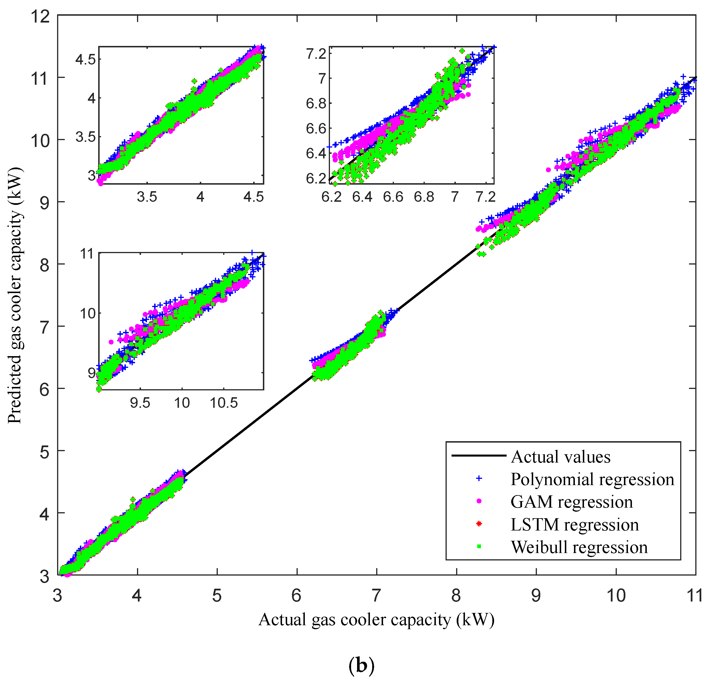
Figure 4b presents the gas cooler capacities predicted by the nonlinear-regression-based models—polynomial, LSTM, GAM, and Weibull—offering an in-depth perspective on their predictive abilities across three specific capacity ranges. In the low-capacity regime, these models also demonstrate impressive overall accuracy. However, in the medium- and high-capacity ranges, a notable trend emerges: the LSTM and Weibull models exhibit greater accuracy compared to the polynomial and GAM models. Both the LSTM and Weibull models perform well in the medium- and high-capacity regimes, indicating their effectiveness in capturing complex patterns within the gas cooler data. The LSTM model, renowned for its ability to handle sequential data, excels at recognizing patterns and dependencies in the cooler’s behavior across various capacities. Meanwhile, the Weibull model, commonly used in reliability analysis, adeptly captures the performance details of the MCGC at higher capacities, outperforming the polynomial and GAM models, which may struggle to adapt to these complexities. The differences in accuracy among these models are attributed to their varying capabilities in modeling the intricate behavior of the gas cooler system.

3.4. Gas Cooler Pressure Drop Predictions

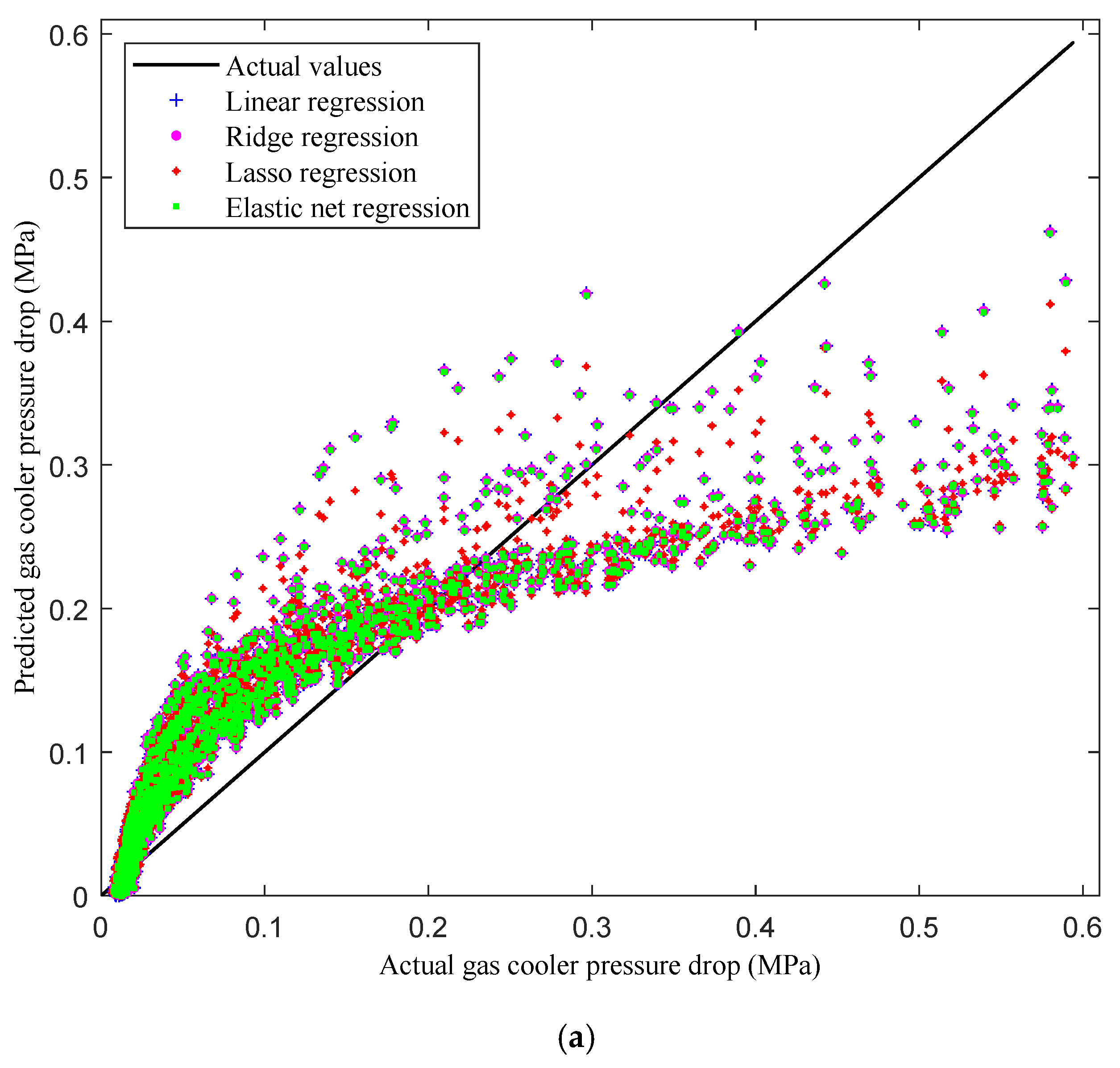
Figure 5a compares the MCGC’s pressure drops predicted by the linear-regression-based models—linear, ridge, lasso, and elastic net—with the actual pressure drop values from the dataset.

An analysis of the performance of each regression model across various pressure ranges reveals some clear patterns. Both the elastic net and lasso models exhibit a distinctive curve: Initially, their predicted pressure drops are higher than the actual ones; however, in the high-pressure regime, their predictions fall below the actual values. Conversely, the pressure drop predictions of the linear and ridge models display a wider spread compared to those of the lasso and elastic net models. Generally, linear-regression-based models struggle to accurately capture the actual pressure drop values owing to their inability to account for the complex, nonlinear relationships between the variables.

The performance of the elastic net and lasso models is influenced by their built-in regularization techniques. Initially, these models fit the training data well, leading to improved predictions. However, as regularization increases, the models become overly simplified, resulting in underestimations [28]. Meanwhile, the greater variation observed in the predictions of the linear and ridge regression models suggests that they struggle when capturing the complex relationships between variables, resulting in less accurate and more dispersed predictions. These findings underscore the limitations of linear-regression-based methods in accurately predicting pressure drop values in the given context.

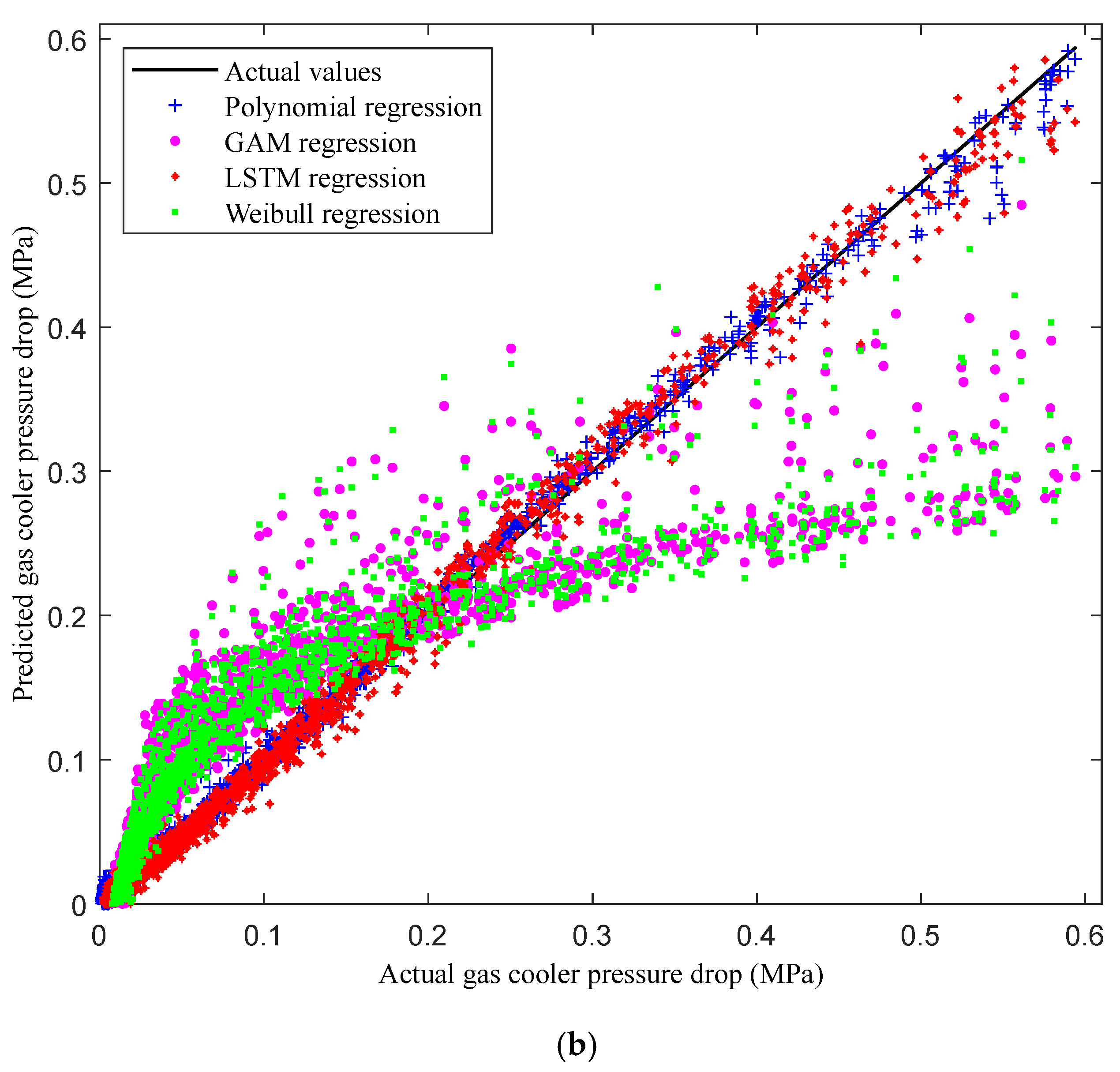
Next, Figure 5b compares the pressure drop predictions of nonlinear-regression-based models—polynomial, GAM, LSTM, and Weibull regression—with the actual values from the test dataset. The results reveal that the nonlinear-regression-based models outperform their linear counterparts in capturing the underlying nonlinear relationships in the data (Figure 5a). Among the nonlinear models, polynomial regression offers the closest fit to the actual values across the entire pressure range, with minimal scatter. This accuracy is attributed to the model’s ability to capture the complex interactions within the pressure drop data, particularly in the medium-pressure regime. Conversely, the Weibull regression and GAM models exhibit greater variance, particularly in the high-pressure range, indicating challenges in fitting more complex, nonlinear relationships under certain conditions.

The LSTM regression model also demonstrates strong predictive capability. Its recurrent architecture allows it to capture complex temporal relationships, resulting in highly accurate predictions across the considered pressure ranges, although minor deviations are still observed in the high-pressure regime.

Comparisons between our nonlinear- and linear-regression-based models (Figure 5a) clearly indicate that the former approaches offer tighter fits with less scatter, thus aligning more closely with the actual values across all considered pressure regimes. The linear-regression-based models, particularly elastic net and lasso regression, tend to overestimate pressure drop values at lower pressures and underestimate them at higher pressures owing to their inherent regularization mechanisms. In contrast, the nonlinear-regression-based models, particularly polynomial and LSTM regression, demonstrate greater consistency and accuracy. This comparison highlights the limitations of linear-regression-based models in capturing the complex, nonlinear behaviors of gas cooler pressure drops and emphasizes the superiority of their nonlinear counterparts in this context.

3.5. Refrigerant (CO₂) Outlet Temperature

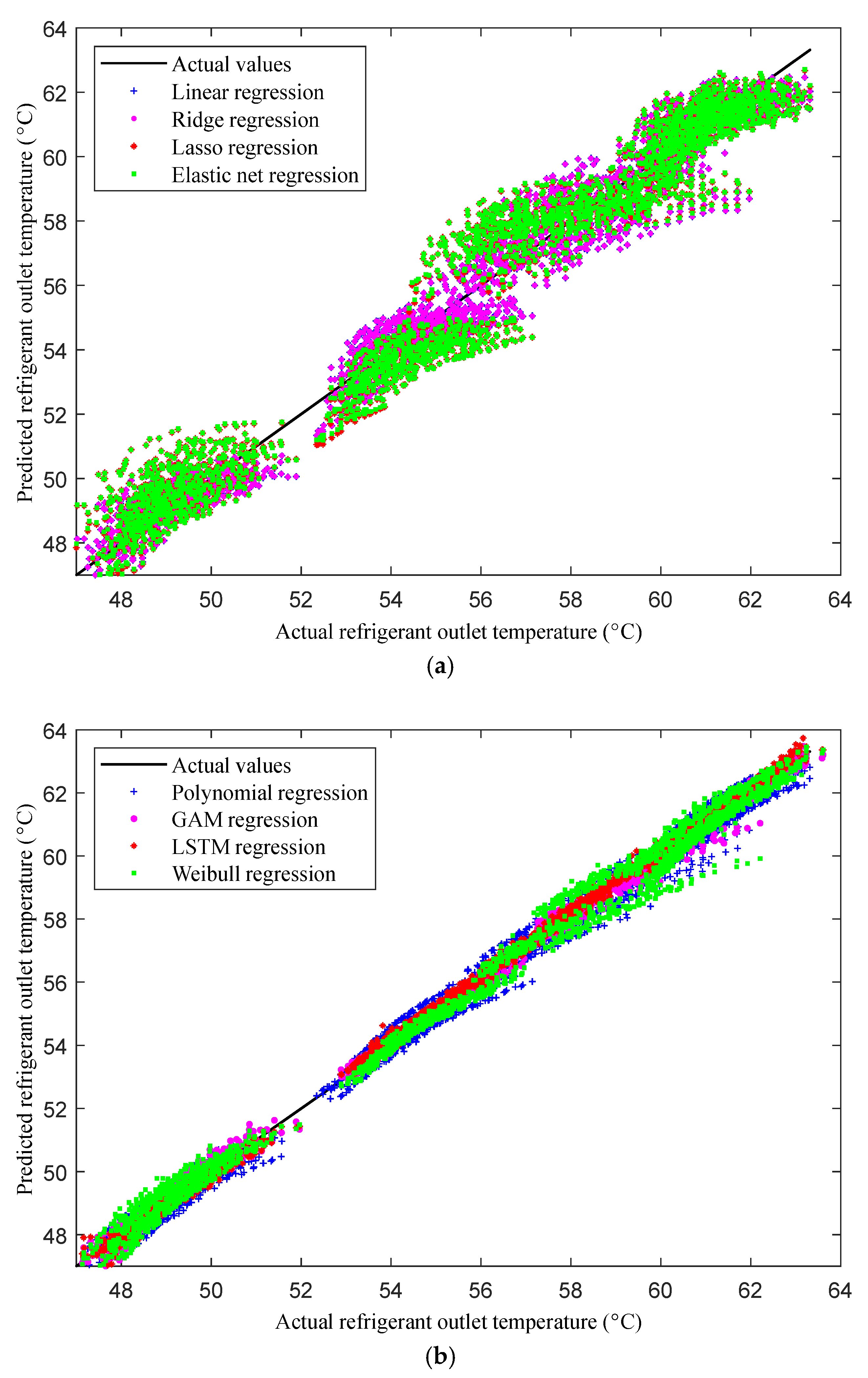
Next, the refrigerant outlet temperature, a critical factor, was predicted using both the linear- and nonlinear-regression-based models, as illustrated in Figure 6a,b.

Figure 6a compares the refrigerant outlet temperature predictions of the linear-regression-based models with the actual temperature values from the test dataset. While these models perform reasonably well, they demonstrate a noticeable deviation from the actual values, resulting in moderate accuracy. This indicates that linear models possess some inherent inconsistencies. Meanwhile, Figure 6b presents the corresponding comparisons for the nonlinear-regression-based models, which consistently outperform their linear counterparts in predicting the refrigerant outlet temperature across the entire dataset. In particular, the LSTM and Weibull models stand out, offering better accuracy compared to the GAM and polynomial regression models. These nonlinear approaches provide more reliable and precise predictions, demonstrating consistent accuracy across different data points.

Given that our refrigerant outlet temperature data exhibit considerable variations, nonlinear-regression-based models—particularly LSTM and Weibull—are ideal for their predictions. These models demonstrate robustness and maintain accuracy across a wide range of data points, making them well suited for scenarios characterized by diverse or changing conditions. However, in situations where predictions are made across a limited data range, both the linear- and nonlinear-regression-based models can yield satisfactory results. The performance disparity between linear and nonlinear models originates from the ability of nonlinear models, such as LSTM and Weibull, to better capture complex patterns and variations in the data. This inherent flexibility allows them to outperform their linear counterparts, which tend to be more rigid and less capable of modeling intricate relationships.

3.6. Air Outlet Temperature

Our next analysis focused on the air outlet temperature predictions of the linear- (Figure 7a) and nonlinear-regression-based models (Figure 7b). Among the linear-regression-based approaches, the lasso and elastic net models demonstrated the best performance, indicating their capability to effectively manage certain complexities within the data that other linear models could not.

However, the predictions of the nonlinear-regression-based models, particularly the polynomial regression model, demonstrated better alignment with the actual air outlet temperatures across the entire dataset. Polynomial regression, renowned for its ability to capture complex relationships within data, emerged as the most accurate predictor in this scenario. The Weibull model closely followed, indicating its effectiveness in managing skewed data distributions. Although the GAM and LSTM models did not outperform the polynomial regression and Weibull models, they still provided reasonably accurate predictions and captured specific nuances within the dataset.

The superior performance of the nonlinear models, particularly the polynomial regression model, implies that the relationship between the predictors and the air outlet temperature is nonlinear. While linear models such as lasso and elastic net are proficient, they may fail to capture such intricate relationships as effectively as their nonlinear counterparts. Consequently, the closer alignment observed between the actual values and the predictions of nonlinear models, particularly polynomial regression, signifies their capability to capture the complexities of this relationship and generate more accurate predictions across the entire range of the dataset.

4. Conclusions

In summary, to identify ML models capable of accurately predicting the performance of MCGCs in CO₂-based automotive air-conditioning systems, we comprehensively compared various linear- and nonlinear-regression-based models. This meticulous evaluation highlighted the superiority of nonlinear models over their linear counterparts. While linear models demonstrated faster processing times, they resulted in higher prediction errors compared to the nonlinear models. Among the investigated models, the LSTM model stood out for its ability to balance efficiency and accuracy effectively. Furthermore, the polynomial regression and Weibull models demonstrated exceptional accuracy across the output parameters.

The ability of nonlinear models to capture the intricate relationships between predictors and output parameters—particularly when predicting air outlet temperature—underscored their suitability for complex data dynamics. Our thorough comparisons delineated the efficacy of nonlinear-regression-based models, which offer precise and reliable predictions for various output parameters of CO₂ MCGC systems. Overall, our findings offer critical insights for future applications of ML techniques, highlighting their potential for evaluating MCGC performance and advancing the optimization of eco-friendly automotive cooling systems.

5. Research Contribution and Future Prospects

This study notably advances the application of ML techniques in predicting the thermohydraulic performance of MCGCs in CO₂-based automotive air-conditioning systems. Unlike previous studies, which primarily relied on experimental and numerical simulations, this study focused on ML models, demonstrating their potential to accurately forecast the critical performance indicators of MCGCs, including gas cooler capacity, pressure drop, and refrigerant and air outlet temperatures. Both the linear and nonlinear ML models adopted in this study overcame the limitations of traditional modeling methods. Nonlinear models such as the LSTM and polynomial regression, in particular, demonstrated superior predictive capabilities. This represents a key methodological advancement in the design of heat exchangers, with specific relevance to automotive applications. Furthermore, the study’s emphasis on CO₂ as a refrigerant aligns with global sustainability efforts aimed at minimizing the environmental impact of automotive air-conditioning systems. The demonstrated capability of ML models to optimize gas cooler performance supports the development of more energy-efficient and eco-friendly cooling technologies for use in the automotive industry.

However, one limitation of this study is the potential risk of overfitting, particularly relevant to models exhibiting excessively high R² values and low MSE scores. Furthermore, the study’s reliance on experimentally validated data could restrict the generalizability of its results to real-world applications. Future research should aim to test these models on a broader range of experimental and real-world datasets to better evaluate their robustness. While this study primarily focuses on traditional regression models to balance simplicity, interpretability, and predictive performance, it also acknowledges the potential of advanced ML techniques such as neural networks and XGBoost in handling more complex, nonlinear relationships in the data. Future research will explore these models to enhance prediction accuracy and assess their applicability, particularly in scenarios where nonlinearity plays a more critical role. Overall, our research findings offer valuable insights for the future optimization of thermal systems, benefiting both the academic research community and the broader automotive industry.