Article

Multi-Objetive Dispatching in Multi-Area Power Systems Using the Fuzzy Satisficing Method

Engineering Department, Universidad Politecnica Salesiana, South Campus, Av. Rumichaca and Av. M. Valverde, Quito 170702, Ecuador
*
Author to whom correspondence should be addressed.
These authors contributed equally to this work.
Energies 2024, 17(20), 5044; https://doi.org/10.3390/en17205044
Submission received: 27 July 2024 / Revised: 25 August 2024 / Accepted: 8 October 2024 / Published: 11 October 2024
(This article belongs to the Special Issue Energy, Electrical and Power Engineering 2024)

Abstract

:
The traditional mathematical models for solving the economic dispatch problem at the generation level primarily focus on minimizing overall operational costs while ensuring demand is met across various periods. However, contemporary power systems integrate a diverse mix of generators from both conventional and renewable energy sources, contributing to economically efficient energy production and playing a pivotal role in reducing greenhouse gas emissions. As the complexity of power systems increases, the scope of economic dispatch must expand to address demand across multiple regions, incorporating a range of objective functions that optimize energy resource utilization, reduce costs, and achieve superior economic and technical outcomes. This paper, therefore, proposes an advanced optimization model designed to determine the hourly power output of various generation units distributed across multiple areas within the power system. The model satisfies the dual objective functions and adheres to stringent technical constraints, effectively framing the problem as a nonlinear programming challenge. Furthermore, an in-depth analysis of the resulting and exchanged energy quantities demonstrates that the model guarantees the hourly demand. Significantly, the system’s efficiency can be further enhanced by increasing the capacity of the interconnection links between areas, thereby generating additional savings that can be reinvested into expanding the links’ capacity. Moreover, the multi-objective model excels not only in meeting the proposed objective functions but also in optimizing energy exchange across the system. This optimization is applicable to various types of energy, including thermal and renewable sources, even those characterized by uncertainty in their primary resources. The model’s ability to effectively manage such uncertainties underscores its robustness, instilling confidence in its applicability and reliability across diverse energy scenarios. This adaptability makes the model a significant contribution to the field, offering a sophisticated tool for optimizing multi-area power systems in a way that balances economic, technical, and environmental considerations.

1. Introduction

Two crucial aspects in electrical energy generation and transmission are the planning of the operation and the supply of the demand. These elements, when combined, form what is known as an economic dispatch of energy. The favorable use of resources, reliability, and sustainability of the system hinge on these factors, making them the focal point of this study in the field of electrical engineering [1,2,3]. Non-conventional energy sources (NCES) in recent years have undergone significant changes in terms of technological advances and are becoming increasingly important in the production of electricity worldwide, mainly due to their almost zero emission of pollutants and also because of their relatively low production costs compared to other types of generation [4,5]. However, due to its highly variable and unpredictable character caused by different factors such as wind density and wind speed for wind turbines or temperature and direct, indirect, and albedo irradiances in the case of photovoltaic panels, among others, it is necessary to create and plan the optimal operation and energy dispatch of this type of generation so that, together with others, there is a cost reduction and optimization of resources to form a robust and reliable electrical system over time [6,7]. It is evident that a thorough analysis of power plant dispatch, considering all relevant factors, is crucial. These include not only the system’s technical restrictions but also the economic aspects, particularly the objective of cost reduction, which is a critical driver in the development of this analysis [8]. Indeed, in most of the analyses of optimal generation dispatch, cost reduction is the primary goal, but a factor that should be equally relevant is reducing greenhouse gas emissions since, as we already know, these are harmful to the planet and its inhabitants; so, this will be taken into account as another of the objective functions of this study [9]. Based on those mentioned above, we can say that the economic dispatch is based on determining the most appropriate option of all the existing generation units to supply the demand of a preset area; however, in real life, it is not possible to isolate an area and work only with it since most power systems have different internal areas connected between them, so it means that an optimal dispatch must take into consideration all the Control Area around it and also all the technical and economic factors that these connections represent, such as the load and generation pattern of each region [10]. The single-area economic dispatch (SAED) is a case study that has been investigated for years. In contrast, the multiple-area economic dispatch (MAED) is a relatively new field that deserves further research, as shown in Figure 1. So, we will delve into this, taking several areas with different types of generation and time-varying loads [10].

2. Background and Related Works

Multi-area economic dispatches (MAEDs) have also become relevant case studies because the need has been detected to create a model that considers the same drawbacks as a SAED but at the same time adapts the constraints of the links and their relevant technical and economic particularities. Since the different world electricity markets are currently seeking to create these connections to optimize their resources and reserves to form a balance between demand and generation and solve their loss problems, MAED also favors the development of dispatch and operation procedures, and encourages the creation of international treaties and agreements [11,12]. Non-conventional energy sources (NCESs) are essential in multi-area dispatches (MAEDs) due to their high uncertainty. Since each area has different environmental characteristics, it is necessary to develop optimal dispatch models that compensate for this variability and ensure reliable and efficient operation of the regional or international system, both economically and technically [13]. Consequently, as mentioned above, electricity system operators must seek methods or mechanisms that predict as accurately as possible the dispatch uncertainties caused by renewable energy generation based on present and future climate changes and also consider the potential growth of demand in each area (Cheng et al. [14,15]). Optimizing energy dispatch in electrical systems is crucial, as it ensures a safe and reliable energy supply while maximizing economic and environmental resources. This reason necessitates comprehensive system operation planning in the short, medium, and long term, considering all possible constraints such as energy balance, generation limits, and transmission capacity. Moreover, it must address the impact of climatic changes and the uncertainty generated by renewable energies, which can be mitigated through mathematical models [16]. The methods created to solve these complex dispatch and planning problems can be heuristic or deterministic. In many cases, they are hybrid due to the system’s many characteristics, variables, and ramifications. There are several models of each type; for example, in the heuristic method, we find the secant method (SM) or also the Artificial Bee Colony (ABC), which is very widely used nowadays, while in the deterministic method, Linear Programming (LP) and all its derivations comprise one of the best known methods. On the other hand, among the hybrid methods are Evolutionary Programming (EP), the famous Particle Swarm Optimization (PSO), and also Fuzzy Logic (FL), on which this paper will focus [17]. Since the method applied in the present study is the fuzzy logic method, it is necessary to detail that it was first used for multi-objective problems in 1978 by the mathematical engineer H J Zimmermann, observing that large-scale multi-objective linear programming problems (LSMLPs) had many gaps and were inaccurate, and he defined it such that the decision maker (DM) can have a fuzzy goal for each of his objective functions. These fuzzy objective functions (FOFs) can be quantified by the membership functions obtained by interaction with the DM [18]. This technique uses a complementary method, as the ε -constraint method conceives broadly. It retains an objective as the primary objective function and transforms the other objectives into constraints, converting the multi-objective problem to a single objective [19]. Therefore, to meet the economic and environmental objectives set out in this paper, this hybrid method of fuzzy logic combined with the ε -constraint method is used to obtain the Pareto front, which will allow determining the optimal solution through the perspective of fuzzy satisfaction, fulfilling the stated objective.

2.1. Electricity Demand Control and Coverage

The increase in electricity demand is constant and random, as new technologies, industries, and urban and rural growth in some sectors are integrated, indicating the importance of planning studies in projecting these scenarios and predicting the energy production necessary to supply them. Supply is primarily aimed at creating a balance between demand and supply, ensuring there is no generation deficit, and, in cases of overproduction, marketing it profitable to cover the investment costs incurred [20]. Therefore, demand will depend on three essential factors [21]: The energy balance, i.e., losses and revenues. The expansion plan in generation, transmission, and distribution. The purchase and sale of energy, based on tariff schedules and marginal cost.

2.2. Power System Operation Planning

The projection or planning of the operation of an electrical system is a global process that is made up of several disciplines that depend on each other for optimal planning; these disciplines observe various points, from the technical, such as electrical power engineering, mathematical–economic, and also telecommunications and computer networks that are of vital importance today for monitoring and automated control over the electrical system. These disciplines are favored in planning so that the energy resource is produced, transported and delivered to the demand in a safe, reliable and economically accessible way [22]. Due to the inherent need for the electrical system to adapt to the load, its analysis becomes a highly complex task. This complexity, however, is not a deterrent but a call for the operator’s expertise. The operator must incorporate programs, procedures, and equipment that facilitate decision making and actions at all stages of the system. A skilled operator establishes a flexible system capable of withstanding internal and external failures, thereby providing reliability and security to the user. In essence, the planning for the operation of the power system is a continuous research path, constantly seeking the most suitable methods for optimization with accurate models for the operation of the power system units. These models consider the physical and operational conditions and restrictions, ensuring their behavior mirrors real-world scenarios [5,23]. With the objective of meeting these assumptions within the planning, stages are established according to the extension of the study period: short-, medium-, and long-term planning [24]; for the development of the present study, it is necessary to deepen the short-term projection, which is detailed below.

Short-Term Projection (STP)

Operational planning is mainly classified according to the time horizon of the model to be followed, so there is short-, medium-, and long-term planning, each with its advantages and disadvantages, but that together form a holistic view of planning [25]. This article will focus on short-term planning, comprising hours to a maximum time of one year; this is transcendental because it considers factors such as possible failures in the generation units, economic dispatch, energy flow, and the daily market [13]. Short-term planning allows the optimization of operating costs, as opposed to long-term planning, which optimizes investment costs. In other words, long-term planning installs the technologies, and short-term planning optimizes the use of these technologies [8]. Then, short-term planning must take into account the system’s current restrictions, such as operating costs, the value and availability of renewable and non-renewable resources, the availability of generating plants, and the capacity of transmission lines in a precise manner and with constant and effective feedback. The operator makes the appropriate decisions that optimize all possible resources and expenses [24].

2.3. Economic Operation

This is called economic dispatch and is based on supplying the demand at the lowest possible cost, i.e., coordinating the production of all available units in such a way that the user can be provided in an uninterrupted and lossless manner but at the same time minimizing operating costs in an optimal way subject to the conditions of the operation and the network. Therefore, finding a solution requires the development of mathematical models that characterize the system to obtain an optimal operational policy for the entry into service of the generation units and the rest of the system and thus benefit the demand. This process for the service of energy supply is called “unit commitment” or economic dispatch [26]. The main problem of the economic dispatch is to foresee all the restrictions of each of the generation units and other elements such as their own operating cost, the use factor in the case of non-conventional energy sources (NCESs), the losses in generation and transmission, the loadability of the lines. It is necessary to take advantage of the advantages and characteristics of each generation plant, such as its geographical location and availability [27,28], considering the coordination between the units belonging to a region and those existing between multiple areas of the same country or region, considering marketing benefits, optimizing the control of shortages and energy overproduction.

2.3.1. Multiple Area Dispatch

The multi-area economic dispatch (MAED) is an evolution of the already known single-area economic dispatch (SAED); this change is related to the growth of demand, which causes parallel increases in generation units and inherently extends geographically due to the growing need for social and industrial development. Consequently, there are variations in and between power systems. Given this approach, creating multi-area dispatch models that mainly seek energy exchange and cost minimization is required, considering each system and subsystem’s own restrictions as well as external restrictions [11]. Different studies [29,30] determine that when there is discordance between the demand and the capacity of an area, it is necessary to adjust the generation repetitively and even inversely with the variation in the load; for this reason, the planning of the dispatch in multiple areas in the short term aims to smooth the daily generation curve, this is obtained by minimizing the standard deviation of the generation series since, in this way, the start-up and regulation cost of the thermal units is reduced, so the output level is constant and ideally flat. Another benefit of short-term planning for multiple areas occurs by simplifying the scheduled generation, thus freeing more resources to regulate the uncertainty of demand and renewable energies incorporated and present in the electrical power systems; it is essential as a transmission method to propose a near-optimal event of minutes or hours of connection between areas, based on the nominal condition, and thus establish the generation interval for each area to be immune to uncertainty.

2.3.2. Multi-Objective Economic Dispatch

Multi-objective optimization models were initially created to satisfy three areas: economic equilibrium, game theory, and pure mathematics, where the main multi-objective approaches are vector optimization and scalarization. There are several methods belonging to each of these approaches, for example, the weighted global criterion method, the lexicographic method, the standard limit intersection method, or the famous Nash Arbitrage and objective product method, guided to the application and formation of the Pareto front. We will base this article on the fuzzy satisficing method [27]. There are several techniques for solving multi-objective economic–environmental dispatches, which can be divided into three categories [15]: The first takes emission as an allowable limit. The second handles emissions as a different target than fuel and operating costs. The third deals with costs and emissions in parallel, viewing the functions as competing and complex objectives. Regardless of their unique characteristics, all three categories of techniques have shown promising results in pursuing multi-objective multi-area dispatch (MAED). This term refers to balancing economic and environmental objectives, a vital research focus across multiple areas. For this reason, the proposed research work considers the type of economic operation that relates not only to an electric system but also to one composed of several areas or regions, turning them into interconnected power systems. The proposed dispatch problem is complex due to the variables and restrictions (technical, economic, and environmental) involved. It is also proposed, within the dispatch problem, the enlistment of multiple objectives that are related within the study with the four independent areas or regions proposed through the methodology selected, in this case, the fuzzy satisfaction method, to find the Pareto optimality based on concepts of the economic dispatch, which considers restrictions associated to the global supply of the demands, reserve restrictions, restrictions of ramps up and down of power of each generator and restrictions of capacity of the link between the different areas. As a result of the multi-objective multi-area optimization problem, the demand–supply is guaranteed in an established period, allowing the evaluation of potential purchases and sales in a multi-area power system environment, involving at the same time the operating costs of the system and those associated with the environmental impact.

2.4. Pareto Front

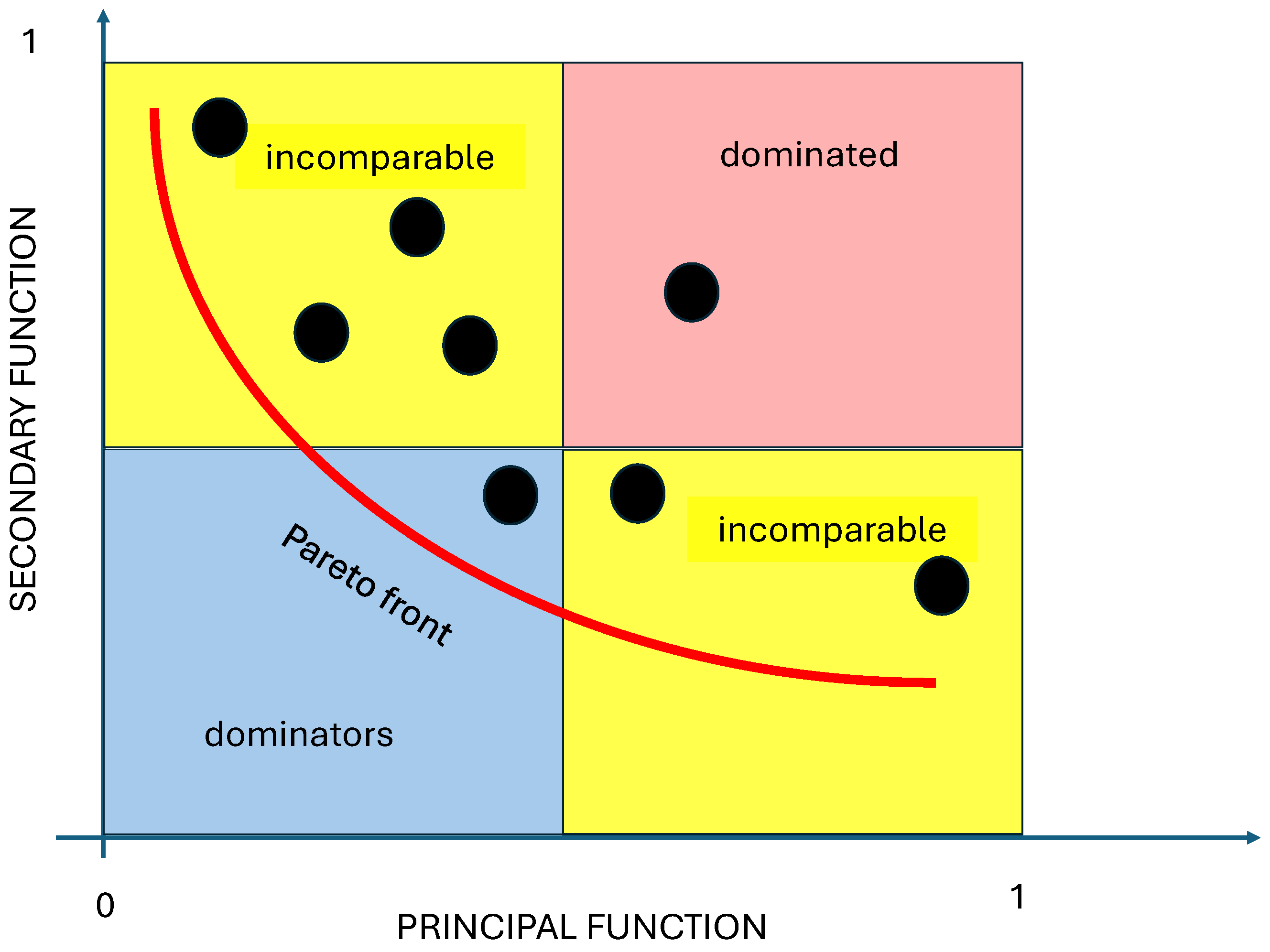
Several procedures exist to solve multiobjective optimization problems, such as the goal programming method or the weighted sum method. However, the Pareto optimization strategy is one of the most widely used. The Pareto front is primarily used because, unlike single-objective models, which have a single solution, multiobjective models have several, so there must be a sweep that can optimally define the best result of all the feasible ones found [29]. An optimal solution does not worsen or improve any objective without simultaneously affecting another. The precision of the Pareto front curve, formed by the primary and secondary objective functions, lies in its ability to pinpoint the feasible responses to the objective functions and identify the optimal solution within these points. This is illustrated in Figure 2, which presents an example of a Pareto curve, demonstrating the effectiveness of this strategy in defining optimal solutions.

Methodologies for Multi-Objective Dispatch Resolution

Several optimization approaches and methodologies, such as mathematical programming techniques and heuristic algorithms, have been utilized to address and solve multi-objective optimization problems. The present study, which is economic–environmental, incorporates a number of objectives, thereby increasing the complexity of the resolution to a significant depth. Conventional mathematical optimization. MAED multi-task economic operation cases, with their intricate complexities and numerous variables, have posed significant challenges to conventional mathematical optimization analyses such as lambda iteration [31], Newton–Raphson [23], and the interior point method. This complexity calls for a more advanced solution. Despite their long-standing use, classical computation-based methods have proven inadequate in determining an optimal Pareto front solution for MAED problems. Their high number of constraints and nonlinear characteristics often lead to premature convergence to a locally optimal result, making them highly sensitive to the system’s initial values. This highlights the urgent need for a more effective approach.
a.
Differential Evolution Method: Differential Evolution (DE) is a relatively recent population technique initially proposed by Storn and Price in 1995 as a heuristic method for minimizing nonlinear, nondifferentiable, continuous spatial functions. The DE algorithm has been applied to various fields of power system optimization [32]. Differential evaluation (DE) belongs to the class of evolutionary algorithms that include Evolutionary Strategies (ESs) and conventional genetic algorithms (CGAs). DE discerns the difference between two randomly chosen vectors from conventional genetic algorithms using perturbing vectors. Differential evolution is a scheme by which it generates test vectors from a set of initial populations. According to [32], when the differential evolution technique is applied to resolve DEMA and the results obtained with the same problem but using a conventional classical method (Newton–Raphson) and a classical heuristic method (Genetic Algorithm) are compared, remarkable benefits are observed.
b.
Particle swarm method: Particle swarm optimization (PSO) has been developed by simulating simplified social models. This algorithm is motivated by the behavior of organisms found in nature, such as flocks of birds or schools of fish, and uses a population-based search procedure. The algorithm probes a space by fitting the trajectories of individual vectors, which are referred to as particles since they are conceptualized as moving points in a multidimensional space. Individual particles are stochastically drawn to the positions of their previous best performance and the previous best performance of their neighbors [33]. The swarm method initializes with a set of random particles and then searches for optima by updating states. Each particle represents a feasible solution to the problem; in other words, each particle represents a point in the multidimensional search space, where the optimal point is to be determined. Each particle changes state around the multidimensional search space until a relatively immutable or optimal state is obtained. Using PSO for MAED solving is easy to implement and design compared to CGAs; however, the number of iterations increases significantly depending on the variables [33].
c.
ε constraint: The epsilon constraint ( ε ) is one of the most used methodologies to solve multiobjective problems; it was proposed in 1975 by Lasdon, Wismer, and Haimes. This technique transforms a multiobjective model into a single-objective one by selecting a primary function and converting the others to constraints associated with epsilon parameters defined by each secondary objective function.
d.
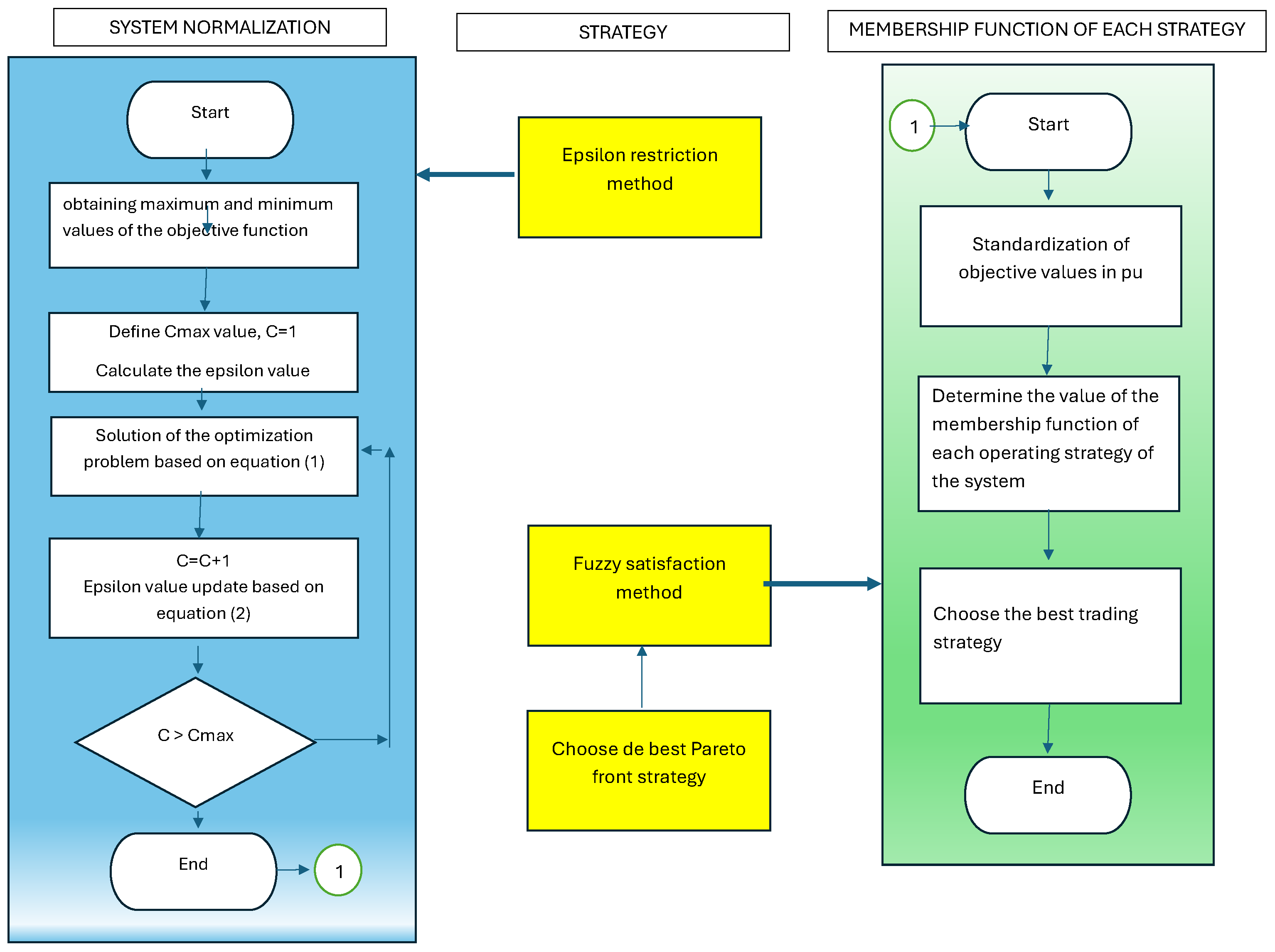
Fuzzy satisficing approach: The fuzzy satisfying approach coordinates the multi-objective model, ensuring a precise trade-off between the preset objective functions. To achieve this, the objective values are first normalized in a unit system. We meticulously calculate the value of the membership function for each system operating strategy, leading us to select the best strategy from all the feasible options. This rigorous process is represented in Figure 3.
The present work developed uses the hybrid method of fuzzy logic complemented with the epsilon constraint to obtain the Pareto front and determine the optimal solution to meet the economic and environmental objectives set to govern the decision making on the generation based on a multi-objective economic dispatch for multiple areas.

3. Mathematical Modeling

The mathematical model, designed to solve the multiobjective dispatch problem in electric power systems across multiple areas, involves formulating equations and inequations. These correspond to a nonlinear programming optimization problem. The model’s outcome, determining the hourly power of various generation units in different system areas, is instrumental in fulfilling the objective functions and, in turn, allows for a comprehensive evaluation of the technical and economic aspects of electricity exchanges between different areas.

3.1. Objective Function Modeling

The optimization model considers two objective functions. The first is associated with minimizing the costs related to operating the generators located in each area, and the second is related to reducing emissions; its formulation corresponds to the following: Operative Costs.
C O T = C g t + C W + C R
where:
  • C O T Total operating cost of the system.
  • C g t Total cost for the production of the thermal generating park.
  • C w Total cost for wind farm production.
  • C R Total cost for the production of the photovoltaic generator farm.
C g t = s = 1 S p = 1 P g G A g , s P g , s , p 2 + B g , s P g , s , p + C g , s
C W = s = 1 S p = 1 P w W ϑ w , s P w , s , p
C R = s = 1 S p = 1 P r R μ r , s P r , s , p
Objective Function: Emissions
E = s = 1 S p = 1 P g G d g , s P g , s , p 2 + e g , s P g , s , p + f g , s
where:
  • S Index of modeled areas.
  • P Time period index.
  • G Index of thermal generators.
  • W Index of wind generators.
  • R Index of photovoltaic generators.
  • P g , s , p Power generated by the thermal generator g located in area s in period p.
  • A g , s Shape factor for the polynomial function of the cost function of the thermal generator g in area s.
  • B g , s Factor of the displacement for the polynomial function of the cost function of the thermal generator g in area s.
  • C g , s Constant for the polynomial function of the cost function of the thermal generator g in area s.
  • P w , s , p Power generated by the wind generator w located in area s in period p.
  • P r , s , p Power generated by photovoltaic generator r located in area s in period p.
  • ϑ w , s Selling price of energy from wind generator w located in area s.
  • μ r , s Selling price of energy from the photovoltaic generator r located in area s.
  • d g , s Shape factor for the polynomial function of the emission function of the thermal generator g in area s.
  • e g , s Factor of the displacement for the polynomial function of the emission function of the thermal generator g in area s.
  • f g , s Constant for the polynomial function of the emission function of the thermal generator g in the area s.

3.2. Applicable Restrictions

The multi-objective problem establishes restrictions associated with the technical characteristics of the generation units, the links that interconnect the various areas, and the supply of demand. For this reason, the restrictions and their description are detailed below.
a.
Demand supply: The restriction guarantees that the energy production, including the contributions of the exchanges between the areas, supplies the demand in each region and for each period.
g G P g , s , p + w W P w , s , p + r R P r , s , p = D s , p + j s S F s , j , p
where:
D s , p Demand in each period p for each area s.
F s , j , p Flow exchanges between area s and area j in every period p.
b.
Flow exchanged between areas: The following inequality ensures that the flow between areas is within the technical limits of the link interconnecting them.
F s , j , p L T s , j S j
where:
L T s , j Technical limit or capacity of the link interconnecting area s with area j.
c.
Bidirectional flow between areas: To model the flow exchange between areas, we establish mathematical formulations representing the bidirectional energy flow within a given hour and its relationship with link capacity. For this purpose, we develop the following restrictions.
L T s , j , p F s , j , p S j
F s , j , p = F j , s , p S j
d.
Technical limitation of generator production: The power dispatched by the generators depends on technical factors associated with their technology. For thermal generators, this means they are constrained by the maximum and minimum limits of their nominal capacity. Similarly, for generators using renewable energies, their production must stay within technical limits and consider the impact of resource utilization. The modeling for both cases is presented in the following formulation.
P g , s , p P g , s m a x
P g , s , p P g , s m i n
P w , s , p P w , s m a x f u w , s
P r , s , p P r , s m a x f u r , s
P w , s , p , P r , s , p 0
where:
P g , s m a x Maximum limit of generator g located in area s.
P r , s m a x Maximum limit of generator r located in area s.
P g , s m i n Minimum limit of generator g located in area s.
P w , s m a x Maximum limit of generator w located in area s.
f U w , s Occurrence of the resource of generator w in area s.
e.
Increase and decrease in generated power: Saved
Generators with thermal technology must consider their technical limitations when increasing or reducing energy production during each hourly period analyzed. We establish the following equations for this purpose.
P g , s , p P g , s , p 1 E g , s
P g , s , p 1 P g , s , p T g , s
where:
E g , s Energy delivery limit of generator g located in area s for each of the periods of time.
T g , s Energy reduction limit of generator g located in area s for each of the periods of time.
f.
System reserve: The supply of the demand in each area must be guaranteed, including the power reserve of each location, whose formulation corresponds to the following:
g G P g , s m a x + w W P w , s m a x f u w , s + r R P r , s m a x f u ( r , s ) ( 1 + r v s ) D s m a x
where:
r v s Percentage of power reserve in area s.
D s m a x Maximum demand in area s.

3.3. Fuzzy Satisfaction and ξ -Constraint

The fuzzy satisficing method solves optimization problems with several objective functions. In this sense, the resolution process begins by solving the mathematical problem model for each objective function, leading to the optimization problem’s multiple resolutions, whose results will allow us to achieve the Pareto front using the constraint ξ ( ξ -constraint). Since the multiobjective optimization problem tends to minimize the objective functions, the following steps will be employed:
1
Solve the optimization problem independently for each of the objective functions.
2
Establish the minimum value of each one of the objective functions for each one of the resolutions carried out.
3
Compute a constraint ( ξ -constraint) for each objective function.
h x ε
4
Vary ε from h x m i n to h x m a x , taking into account the number of events to simulate (n), maximizing in each event the h x , based on the following formulation.
ε x = h x m a x + ( h x m i n h x m a x ) A i A n
where:
A i : Corresponding value of the counter to define a point of the Pareto front.
A n : Total of the events evaluated in the counter.
5
Each value obtained by solving each event using ξ -constraint belongs to a solution of the optimization model.
6
The Pareto front will be formed by the number of values obtained using ξ -constraint.
Once we determine the Pareto frontier, the fuzzy satisfaction methodology will establish the optimal value that equitably satisfies the objective functions. This methodology uses a relevance function to indicate how strongly each element of a given universe belongs to that set. We describe its general formulation below.
σ h x ( F γ ) = 0 h x m a x h x ( F γ ) h x m a x h x m i n if h x m i n h x ( F γ ) h x m a x
Finally, the fuzzy satisficing method will maximize the minimum satisficing among all the objective functions, expressed by the following formulation.
z = m a x ( m i n σ h x ( F γ ) )

3.4. Pseudocode

As described in Table 1, you must follow some phases sequentially to apply the mathematical model and obtain its resolution. You can extrapolate the application of the phases independently of the scalability of the problem to be solved.

4. Model Application

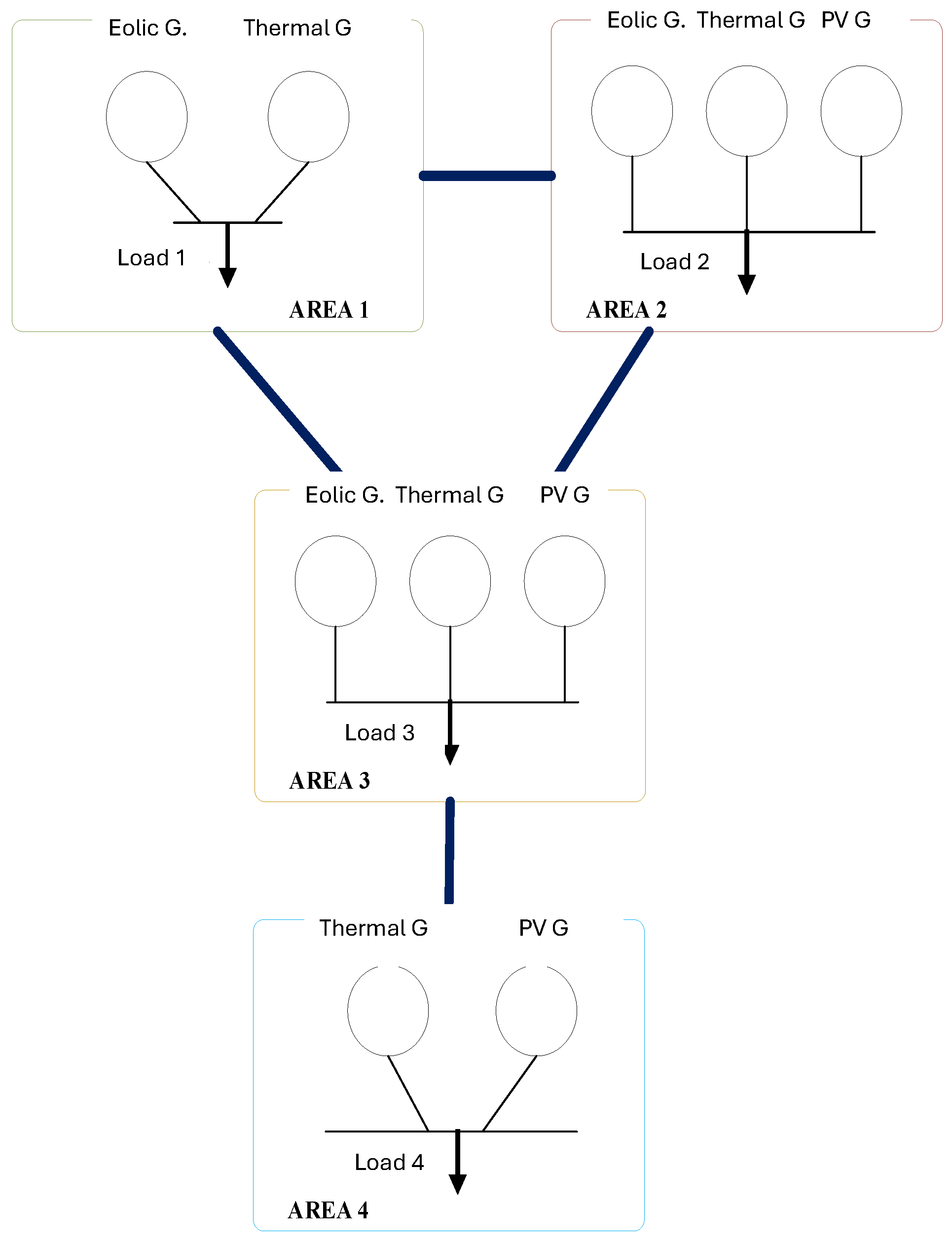
The number of areas to be modeled will amount to four, which will contain a generating park with different technologies, an hourly demand for a 24-h period, and additional interconnected areas, as shown in Figure 4.

4.1. Power Generating Plant

Table 2 shows the location and technology of the generators to be used and their allocation in each of the four areas.
The generating park with thermal technology obtained the data and parameters, independent of its location, by considering [30], presented in Table 3.
The cost function coefficients were obtained as established in [30] and showed in Table 4. In contrast, the factors associated with the emissions are obtained using the factors that consider the British thermal unit (BTU), as described in [34]. The coefficients for costs and emissions are given in Table 5 and Table 6, respectively.
Based on what is described in Table 5, the conversion factor Y g obtained according to [34] is used to determine the emission coefficients; the conversion factor is detailed in Table 6.
For generators using renewable energies, the data, and economic and technical scope parameters have been those considered by the U.S. Energy Information Administration, detailed in Table 7.
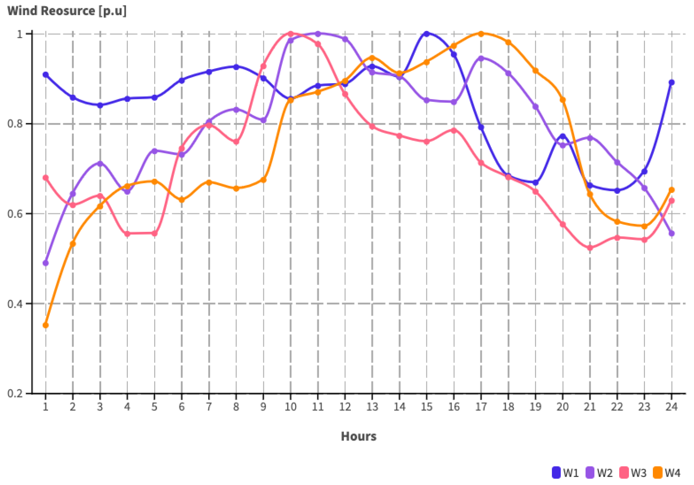
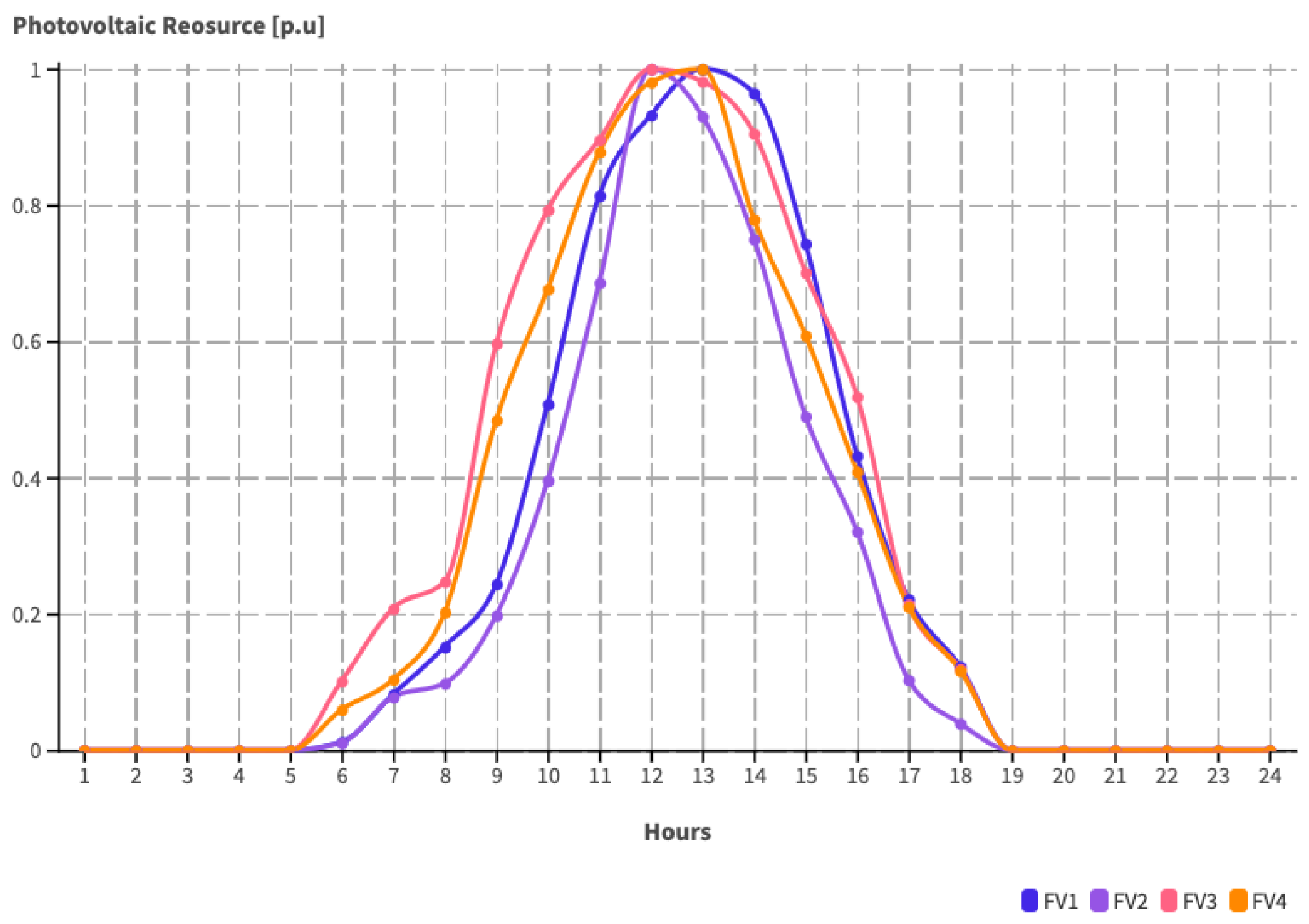
In addition to the above, we have tabulated the probability of the energy resource of renewable energies being modeled as described in [35], which are detailed in Figure 5 and Figure 6, according to the type of technology.

4.2. Demand

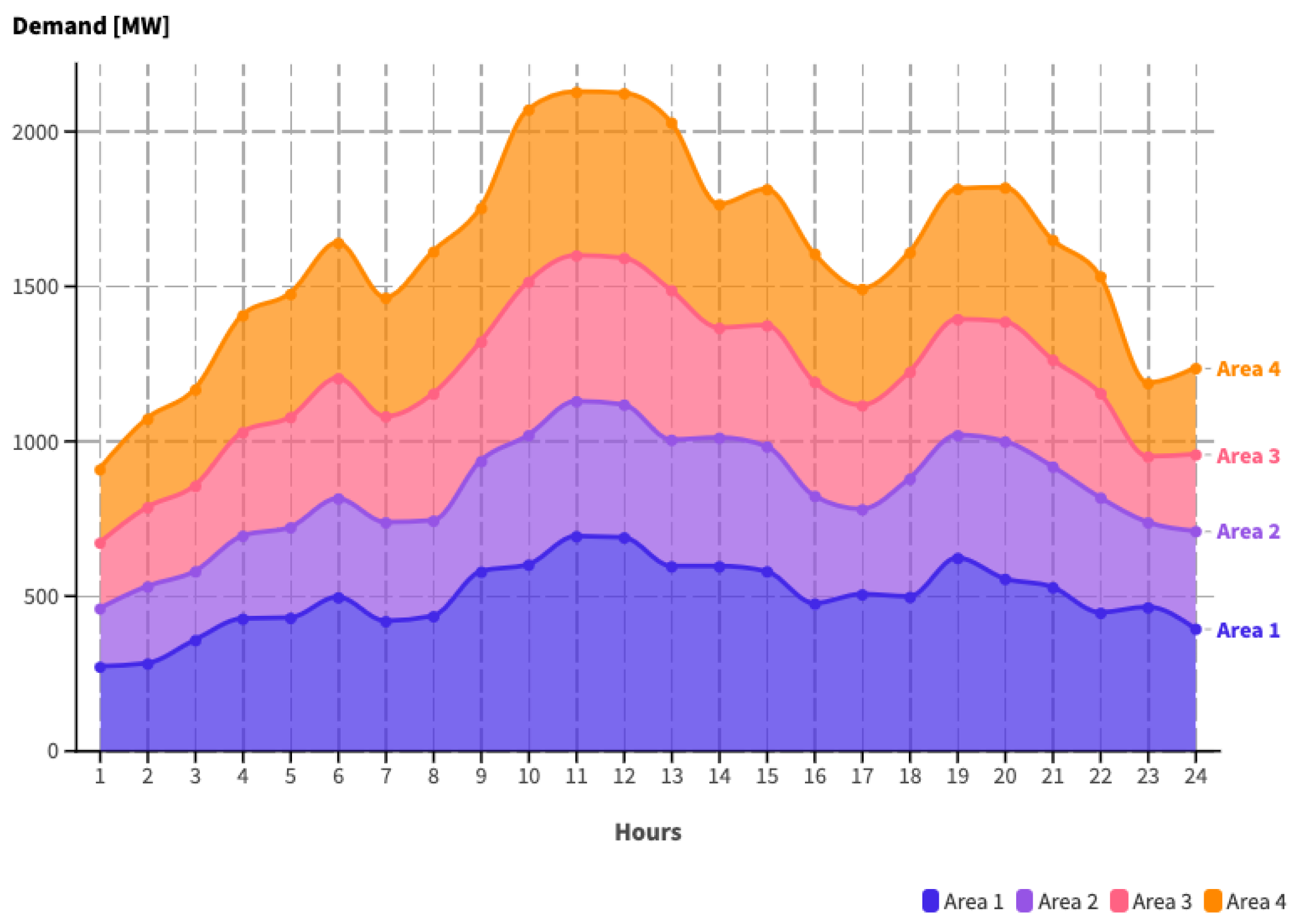
In this section, we show the demand for each period to be supplied, whose values are compiled from [36], resulting in Figure 7.

4.3. Links between Areas

Figure 4 describes the general scheme of the system to be modeled, which shows the interconnection of areas. For the modeling, it is necessary to know the capacities of the links, which are shown in Table 8, and whose values are referenced according to [37].

4.4. Study Case

We propose three studies or cases to apply the multi-objective optimization model. These studies will help us establish feasible technical and economic results for solving the mathematical problem. We will compare and analyze the results of these studies to provide a comprehensive understanding of the optimization process.
i
Case 1: In this study, we carry out energy dispatch in each area, allowing the generators to supply the demand autonomously and independently. Consequently, we do not model the interconnection of the areas. We will compare the resulting values of this study with those from the other two studies to validate the economic and technical parameters. We do not consider multi-objective modeling in this study.
ii
Case 2: In this case, we will model the interconnection of the different proposed areas, allowing us to understand the generators’ interaction in supplying demand in each area. We do not consider multi-objective modeling in this study. We will analyze and evaluate the economic and energy results by comparing them with cases 1 and 3, quantifying technical and economic variables.
iii
Case 3: This case will model the multi-objective problem, and additional areas will be interconnected; these premises’ interaction must guarantee each area’s global and individual demand. The results will be compared with those obtained in cases 1 and 2.

4.5. Parameters for Studies

The studies described in the previous paragraph must consider the following parameters.
  • Area 1 consists of four thermal-type generators with a total capacity of 870 MW and a wind unit with a capacity of 380 MW. It is interconnected with areas 2 and 3.
  • Area 2 consists of three thermal generators with a total capacity of 630 MW, a photovoltaic generator with a capacity of 150 MW, and a wind generator with a capacity of 270 MW; it is interconnected with areas 1 and 3.
  • Area 3 has a generator park with four thermal generators, each with a total capacity of 650 MW, two wind units, each with a capacity of 300 MW and 330 MW, and a 180 MW photovoltaic unit.
  • Area 4 has a 680 MW generator park with thermal technology and two photovoltaic generators of 100 and 140 MW; it is interconnected only with area 3.

5. Analysis of Results

In this section, we will analyze the results for each of the proposed studies. This analysis is complex and in-depth, leading to the results of the energy and economic variables, the details of which are shown below.

5.1. Case 1

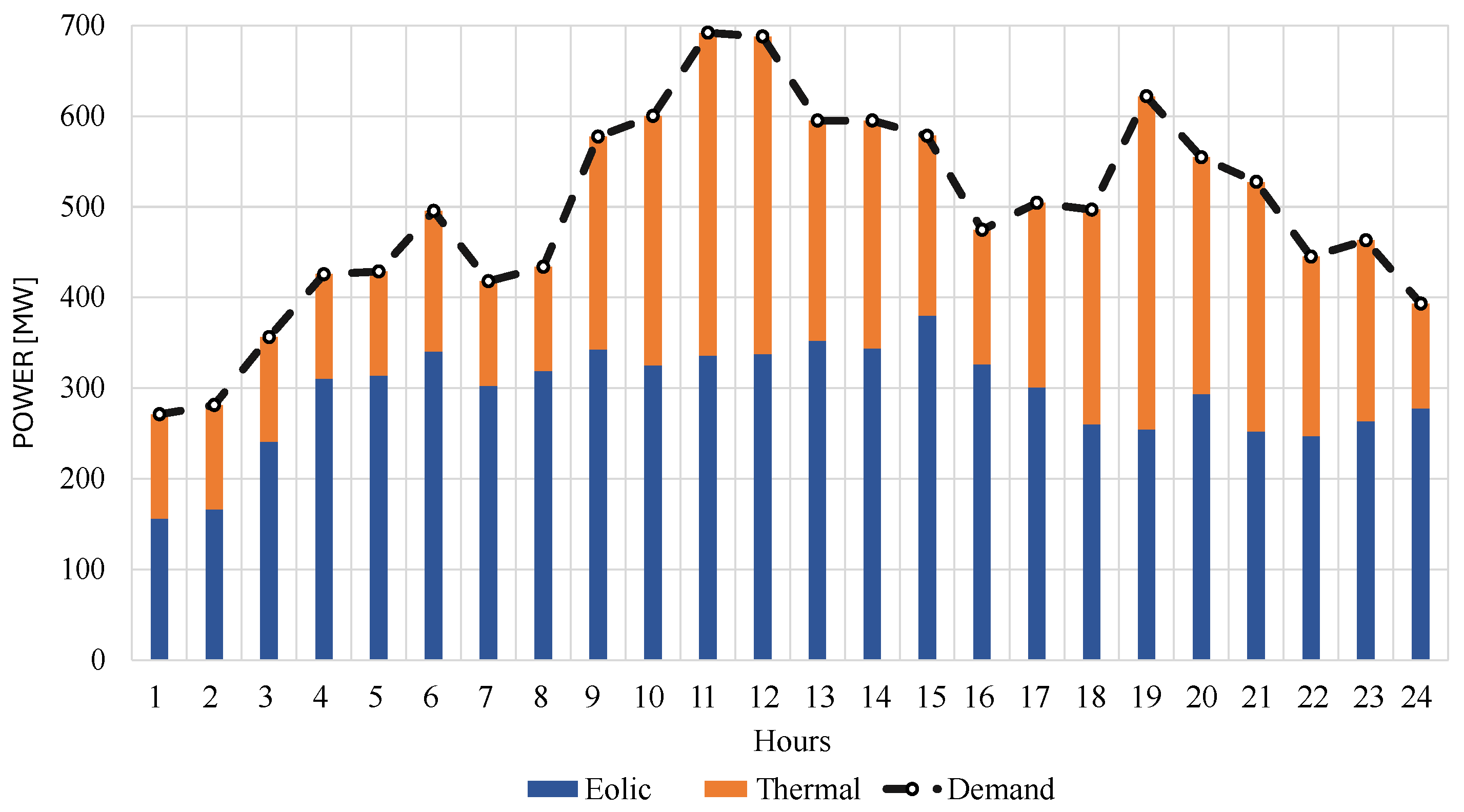
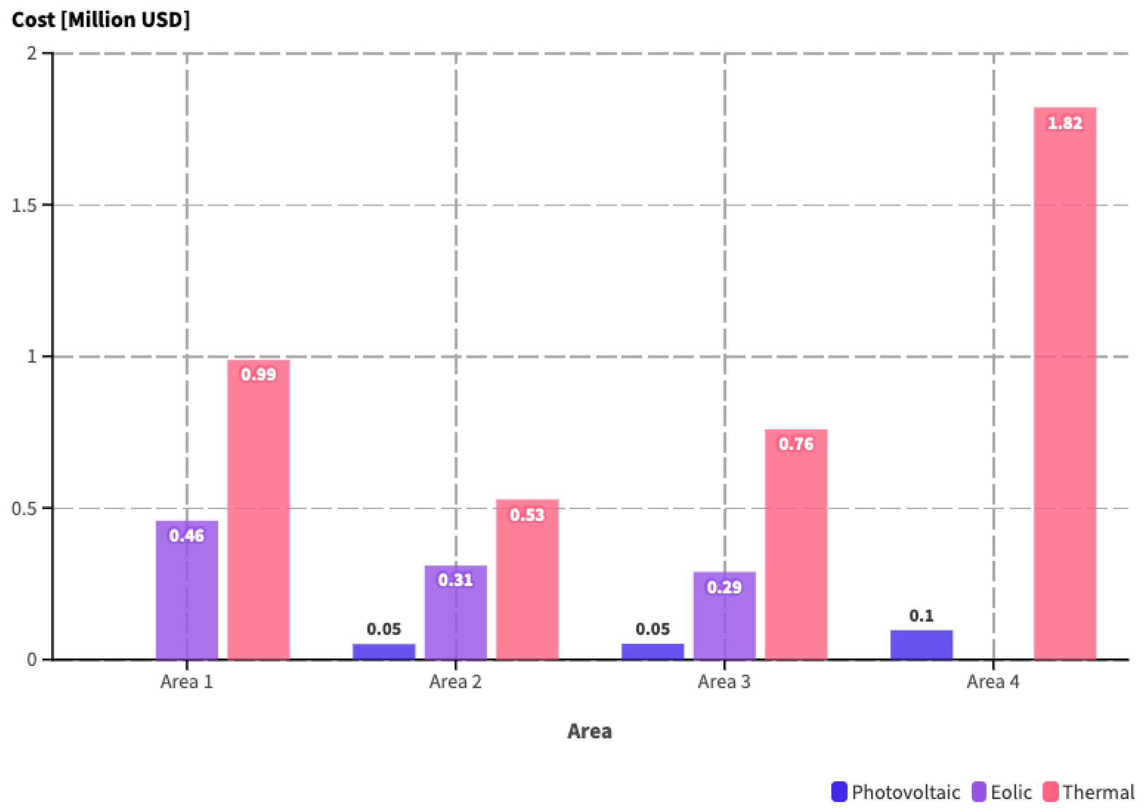
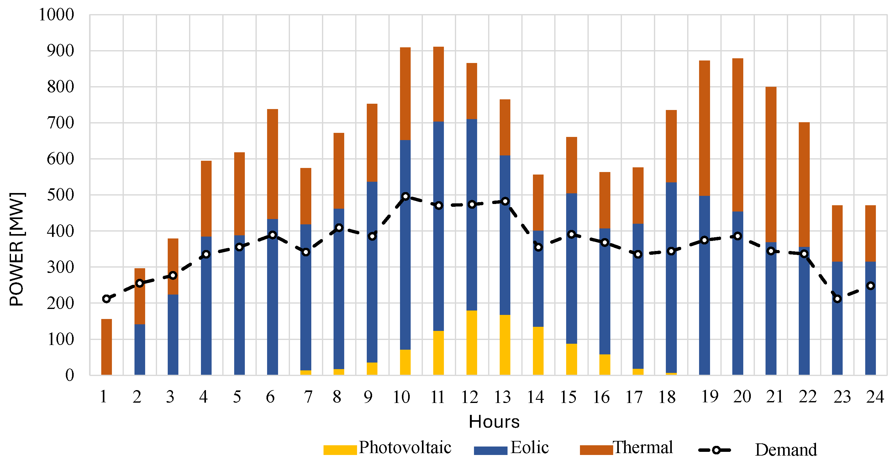
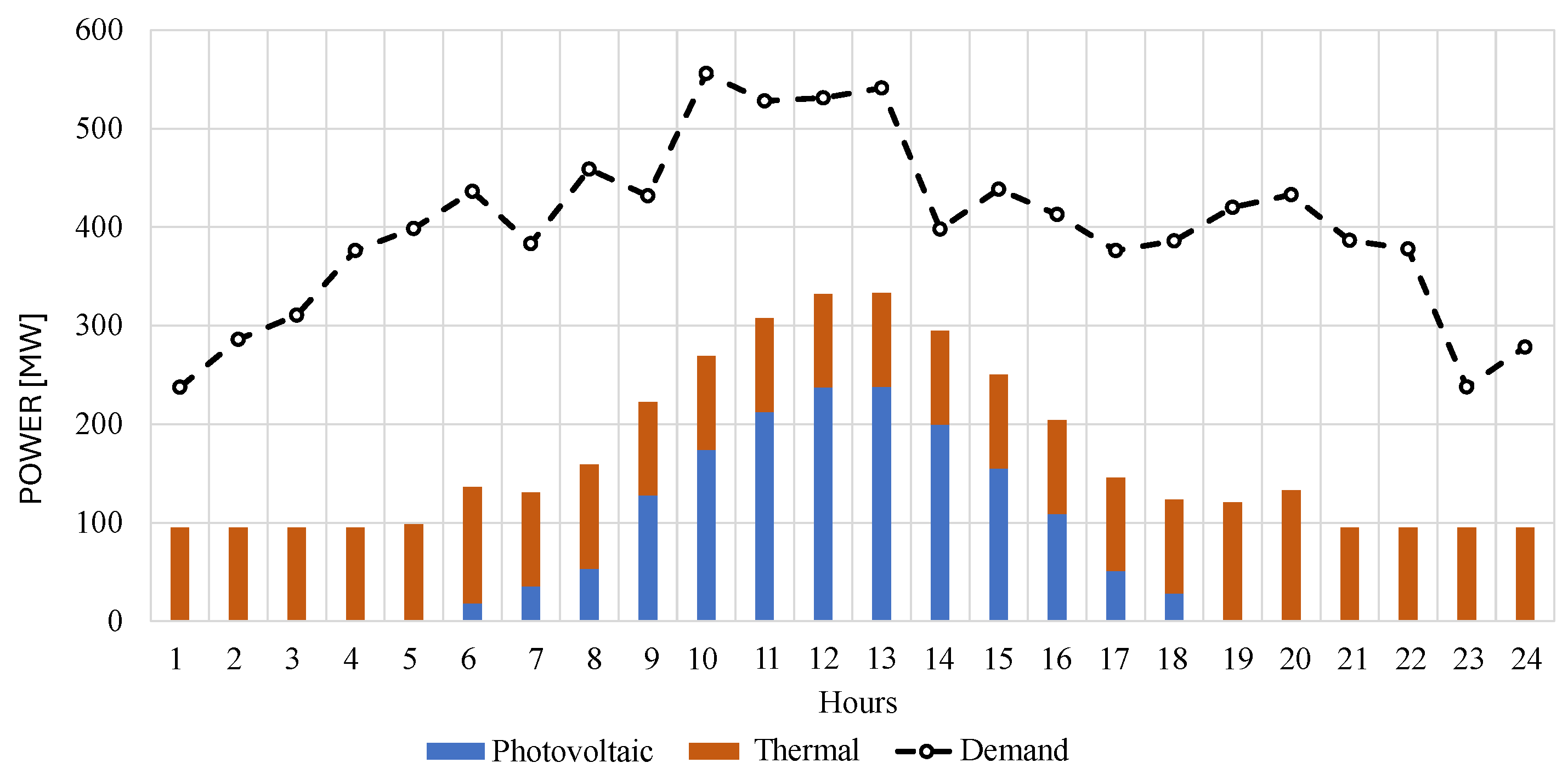
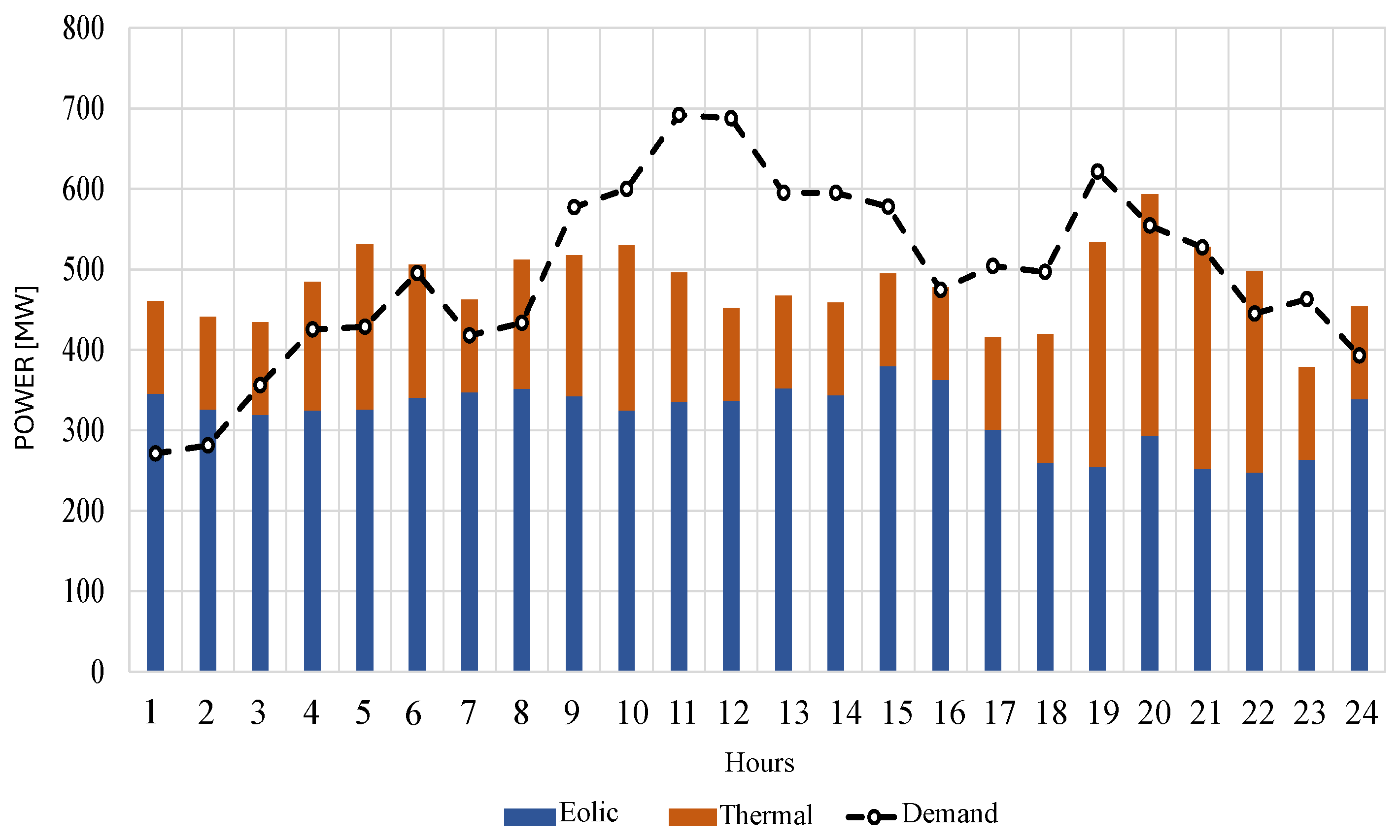
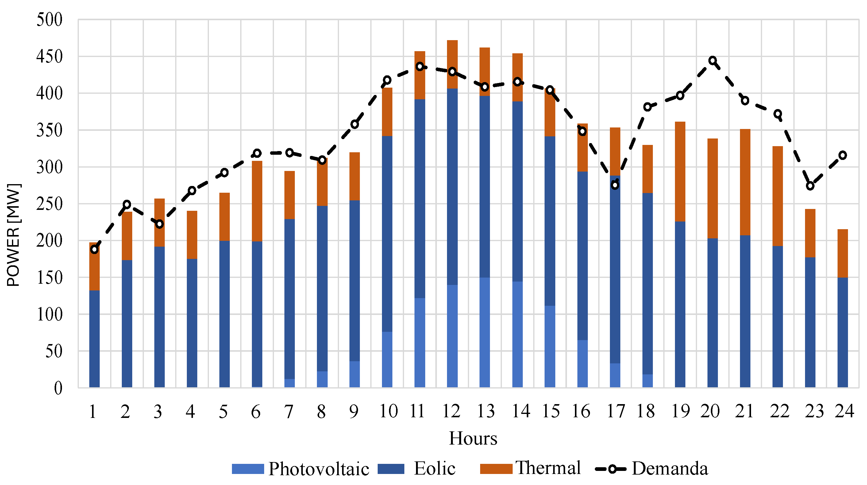
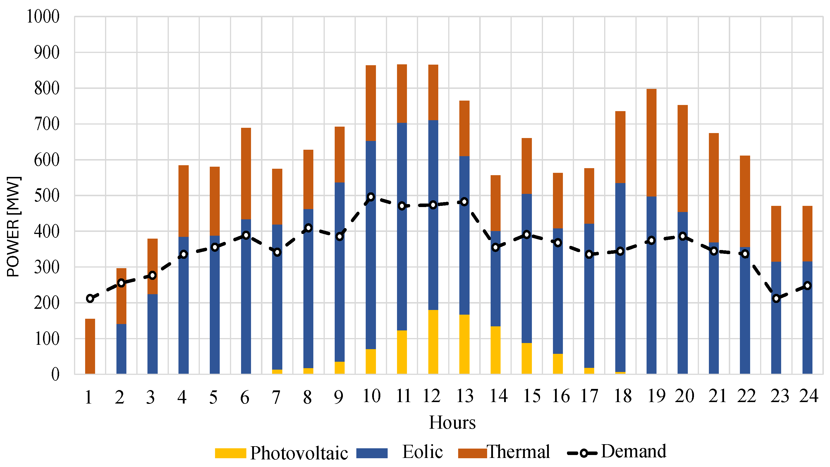
According to economic dispatch, the supply of the demand for each area autonomously by its generation park determines the values of the energy and financial variables. Therefore, the following illustrations Figure 8, Figure 9, Figure 10 and Figure 11 show each area’s dispatch and type of technology.
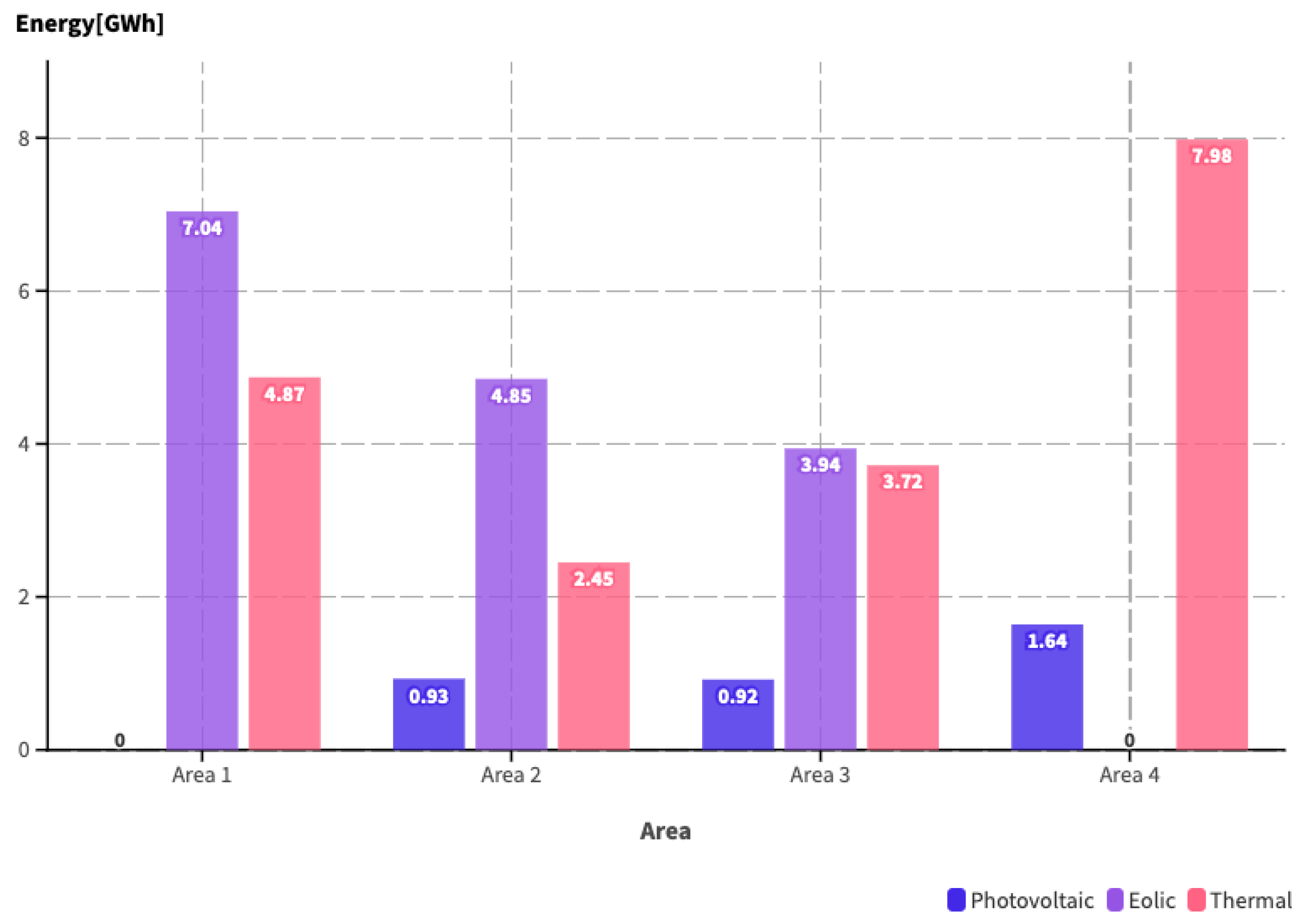
As shown in the previous figures, the energy production of the generating park in each area is dispatched economically and guarantees the autonomous supply of demand. Figure 12 shows the energy blocks for each area and the technology to supply the autonomous demand.
This also shows that of the total energy, photovoltaic energy represents 9.1%, wind energy is equivalent to 41.3%, and energy from thermal generators amounts to 49.6%. The illustration shows values by energy block, by area, and by technology. From the energy production resulting from the autonomous supply dispatch, we evaluate the economic values derived from the energy production associated with area and technology.
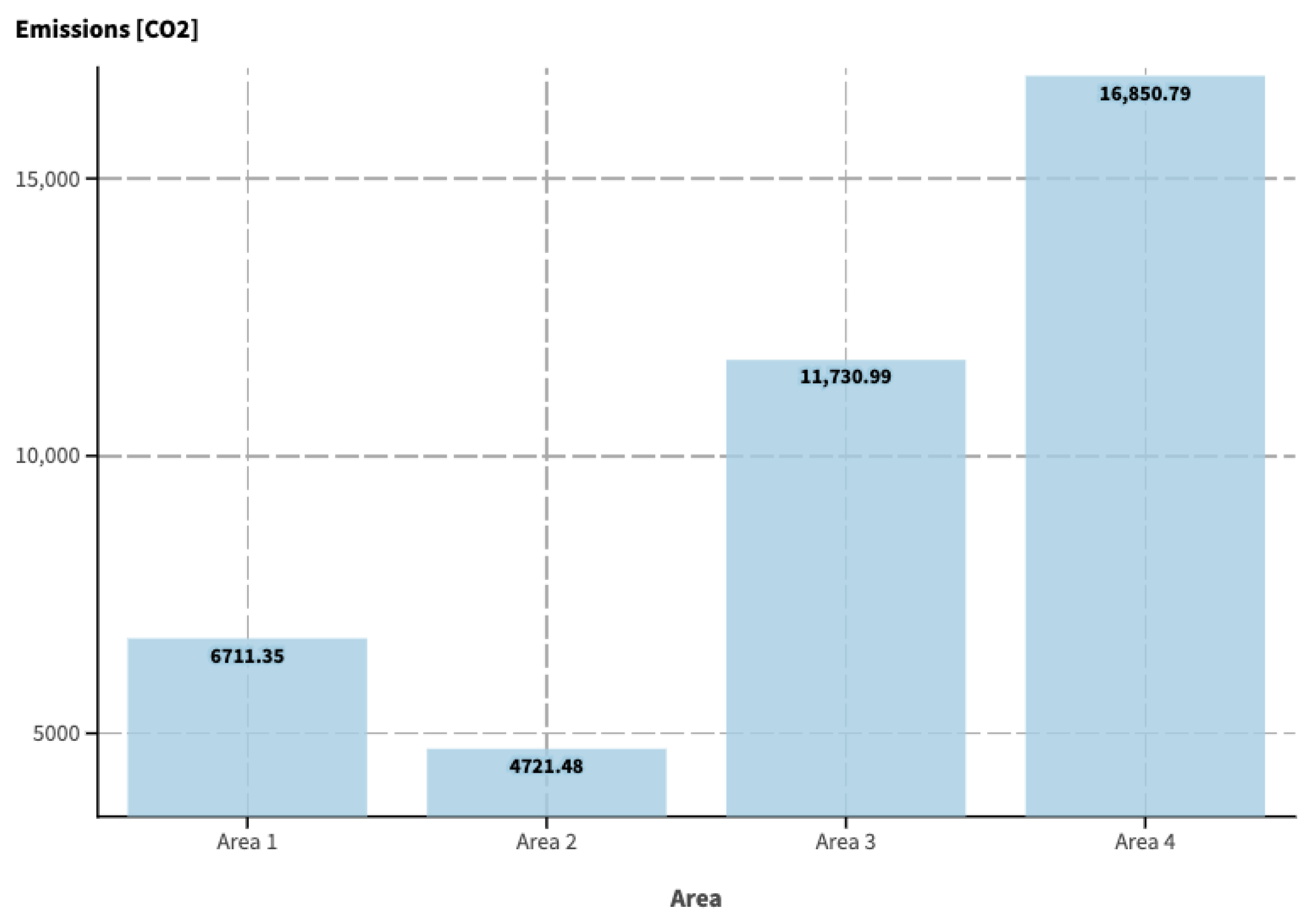
From Figure 13, 76.5% of the total cost corresponds to thermal generation, while 19.7% corresponds to the cost of wind generation, and 3.7% is the percentage of the cost of photovoltaic generation. Finally, the CO 2 emissions derived from the production of energy from thermal generators are evaluated, as a result of which, for each area, the amount of emissions is shown in Figure 14.
Figure 14 shows that the highest percentage of emissions, at 42%, are produced in area 4; area 2 produces the most minor emissions, with a rate of 12%. The percentages are calculated based on the total 40,014.00 tons of CO2.

5.2. Case 2

In this study, we will interconnect the four modeled areas and perform the economic dispatch. This modeling will result in the dispatched generation and the exchanges between areas that displace costly generation production. For this reason, the dispatch carried out in each region is shown in the following illustrations.
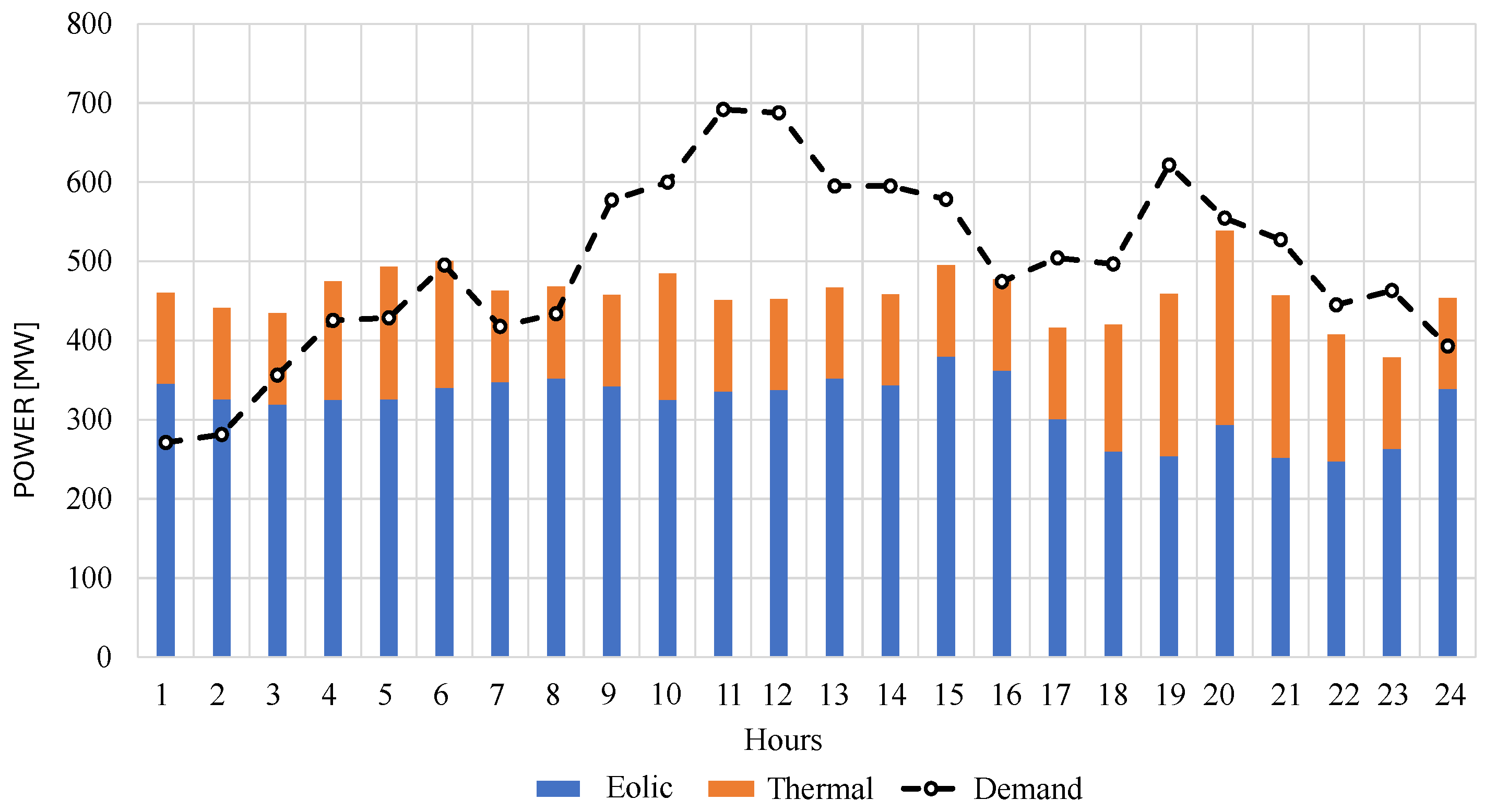
Figure 15 shows that we reduce generation in area 1 most of the time because we supply demand from the interconnected regions. However, in the morning, we can deduce that generator park 1 provides energy to the interlinked areas. Figure 16 shows this energy exchange.
Also, we proceed to determine the net values in the delivery or reception of energy concerning area 1, the results of which are presented in Table 9, from which it is observed that area 1 receives 904.78 MWh in the period under analysis.
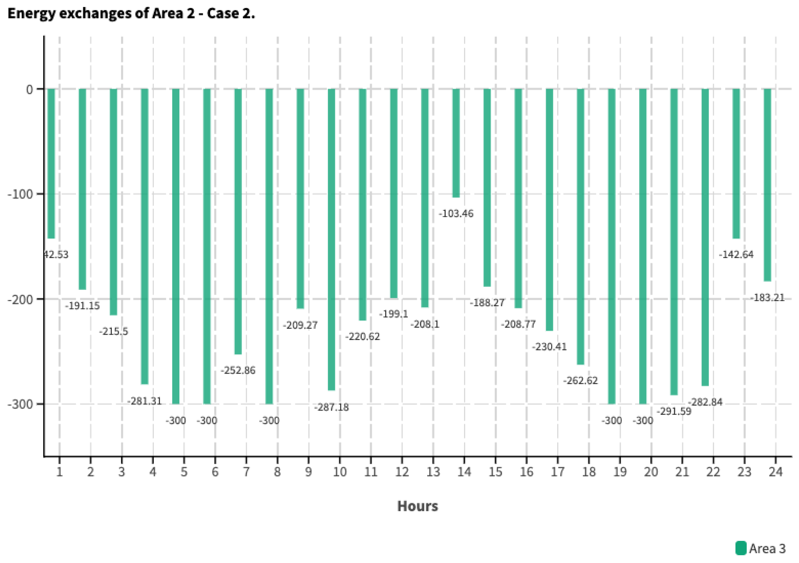
Figure 17 shows that, in the period of maximum demand, area 2 takes energy from the interconnected areas, while, in periods of medium demand, area 2 delivers energy to the other areas. The energy exchange is shown in Table 10.
Likewise, the analysis is carried out for area 3, resulting in the economic dispatch. Figure 16 shows that, in the period of maximum demand, area 2 takes energy from the interconnected areas, while, in periods of medium demand, area 2 delivers energy to the other areas. The energy exchange is shown in Figure 18.
This also shows that the net between the energy received and delivered corresponds to the value of energy received; Table 11 shows the details of the above.
The analysis of area 3 is carried out similarly, resulting in the economic dispatch shown in Figure 19.
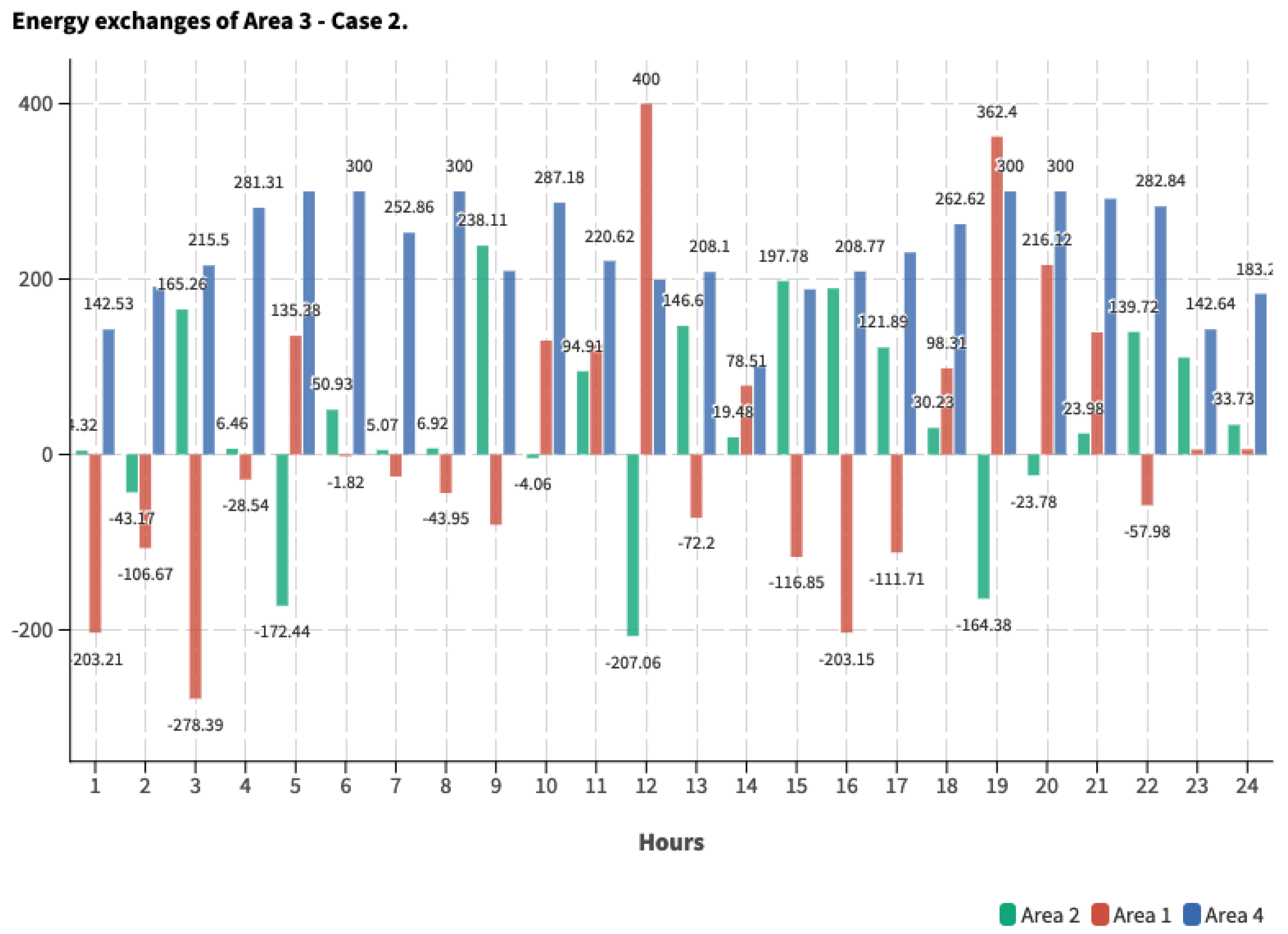
This also shows that this area exports most of the energy to the four areas. Since most of the energy produced corresponds to economic energy, Figure 20 describes the energy exchanges to the other areas, and it shows that although area 3 receives energy sporadically, during most of the analysis period, it delivers energy mainly to area 4; the net value between energy received and delivered corresponds to a value of delivered energy.
The analysis of area 4 is carried out similarly, resulting in the economic dispatch shown in Figure 21.
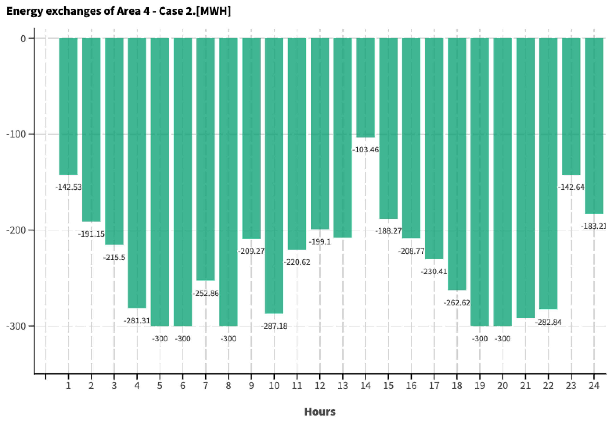
It also shows that this area imports most of the energy from area 3 since most of the energy produced corresponds to economic energy. To establish the energy exchanges with the other regions, their values are described in Figure 22.
It also shows a significant import from area 3; the net value between energy received and delivered corresponds to the value received, as is shown in Table 12.
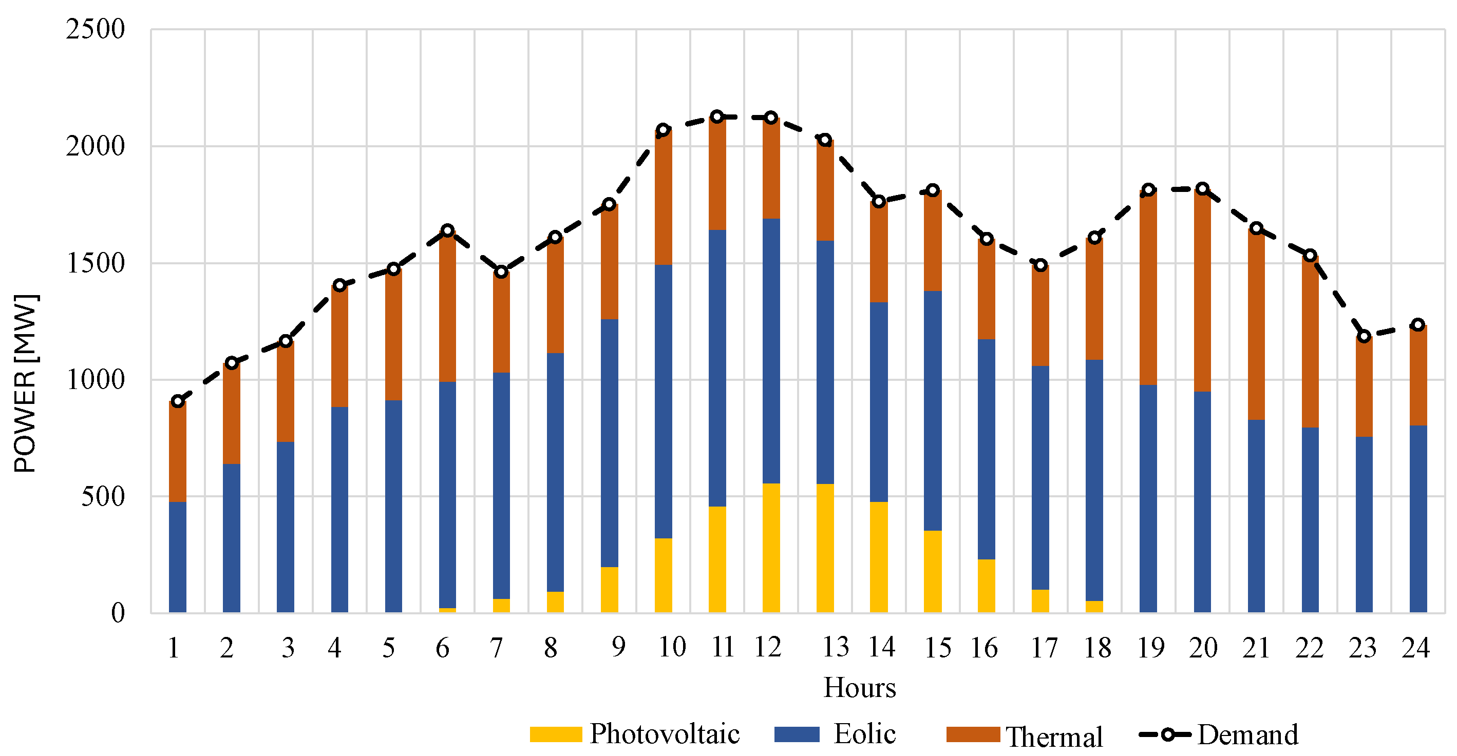
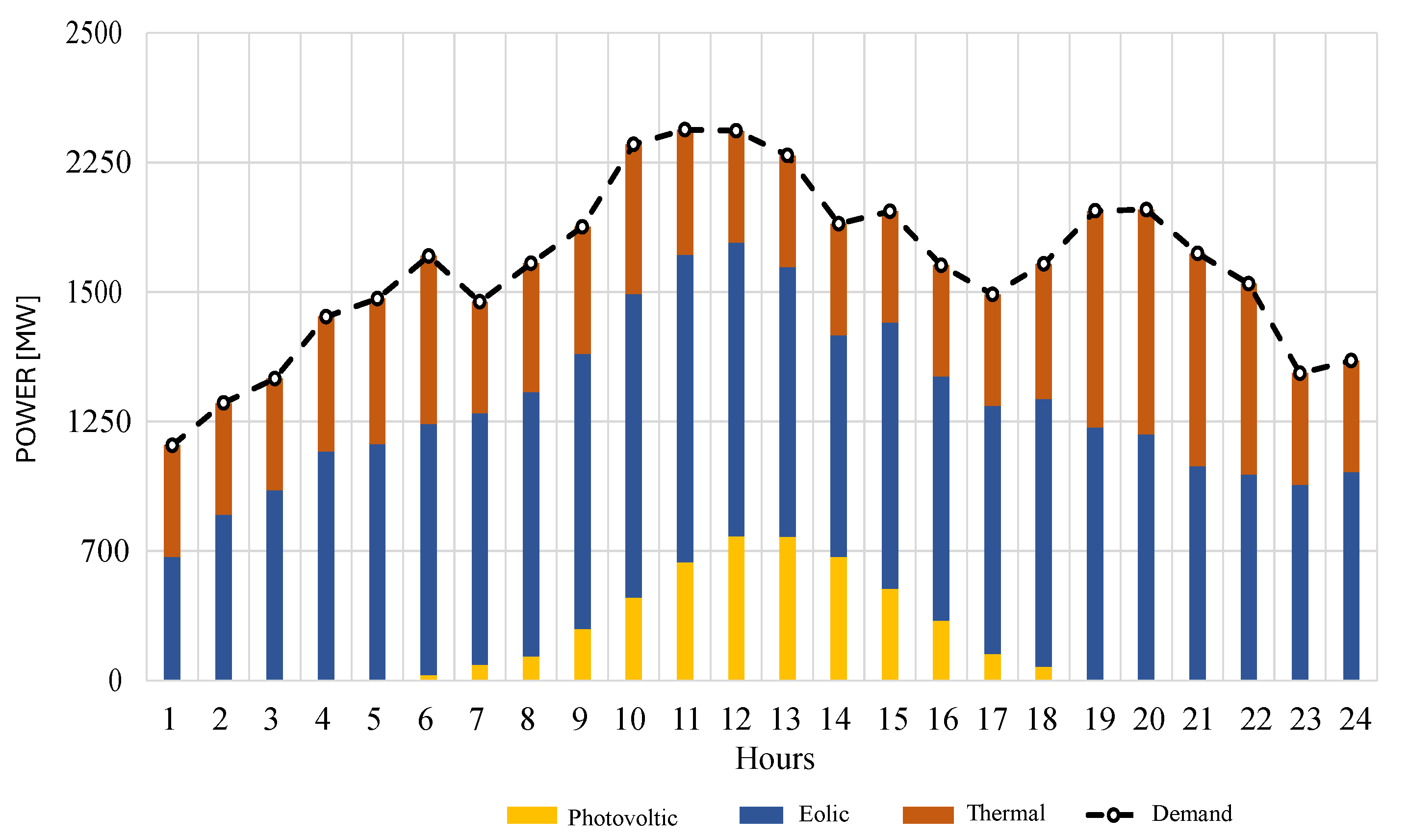
After carrying out the individual analysis by area, it is necessary to illustrate the global supply in which the energy exchanges between areas are included, as shown in Figure 23.
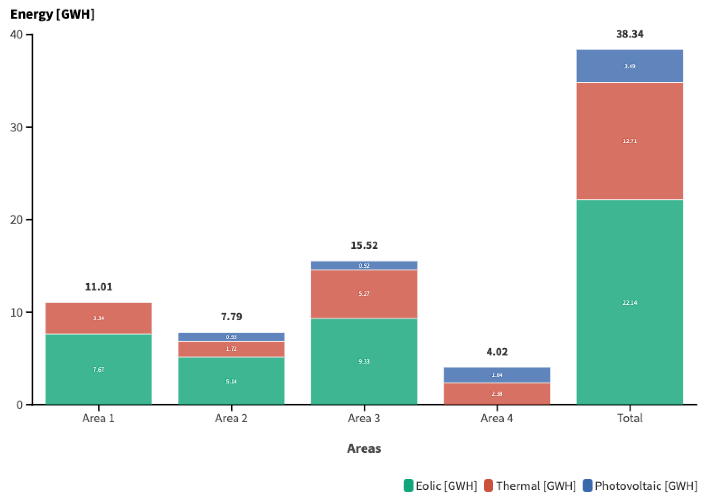
It also demonstrates that the multi-area dispatch effectively fulfills the global demand. Next, we will present the energy blocks by type of technology for each area as shown in Figure 24.
From the energy production resulting from the interconnected supply dispatch, we evaluate the economic values derived from the energy production associated by area and technology.
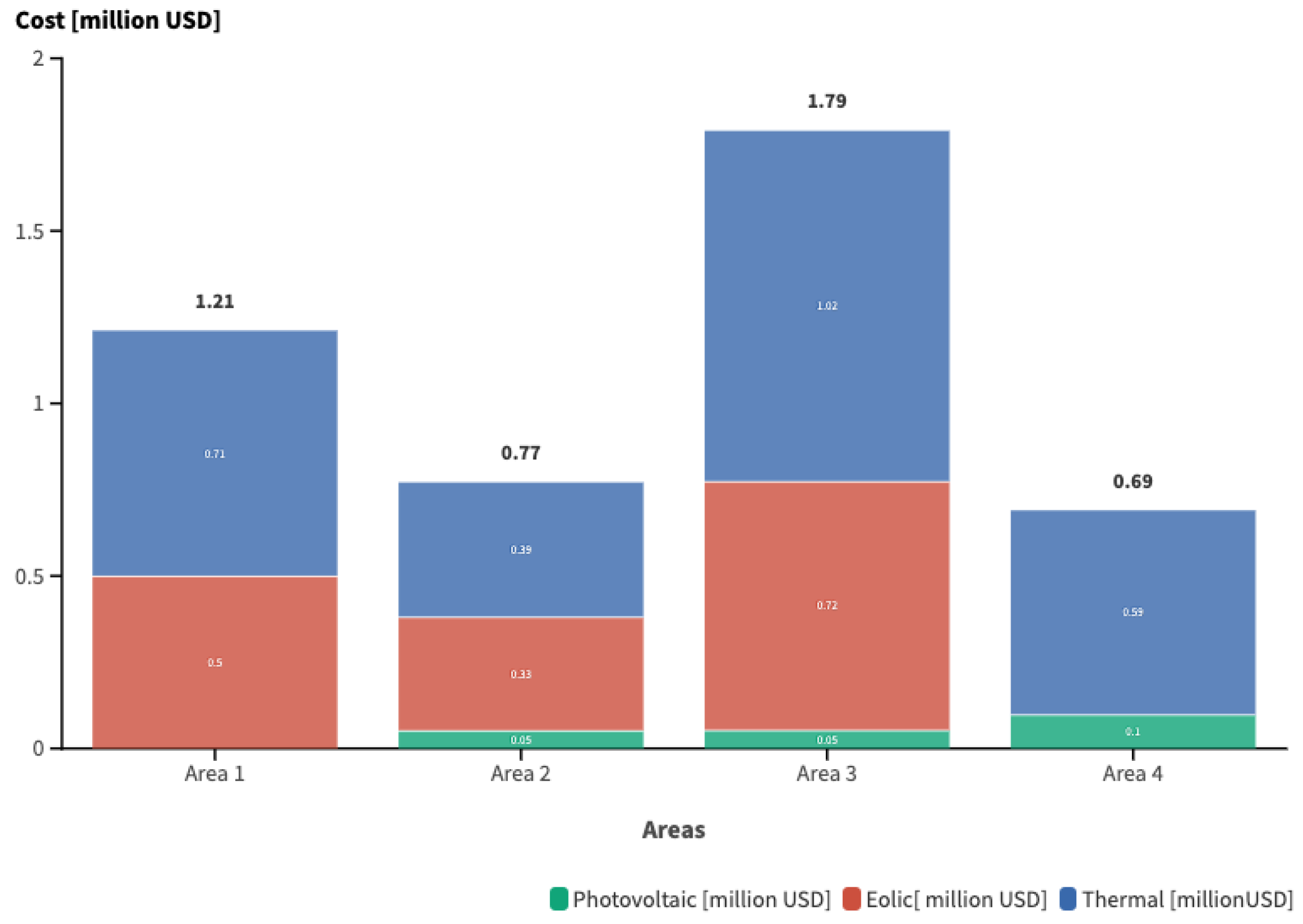
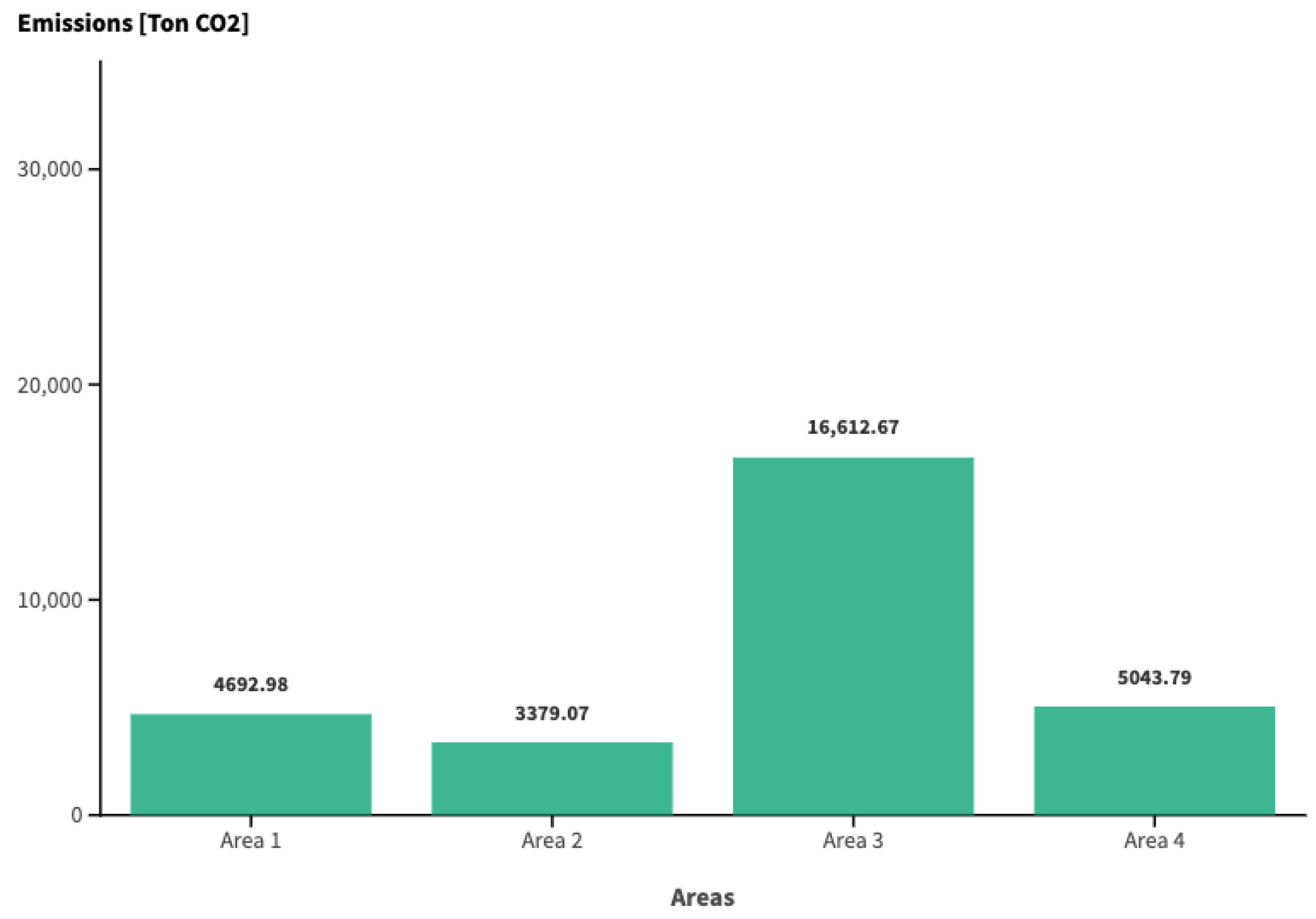
From Figure 25, 60.8% of the total cost corresponds to thermal generation, while 34.7% corresponds to the cost of wind generation and 4.5% is the percentage of the cost of photovoltaic generation. Finally, we evaluate the amount of CO 2 emissions produced by energy from thermal generators, with the results shown in Figure 26.
It also shows that compared to Study 1, total emissions are minimized by 26%, resulting in a total value of 29,728.50 [tons] of CO 2 . Of this value, 56% corresponds to emissions from area 3, while area 2 produces the minimum amount of emissions, which amounts to 11%.

5.3. Study Case 3

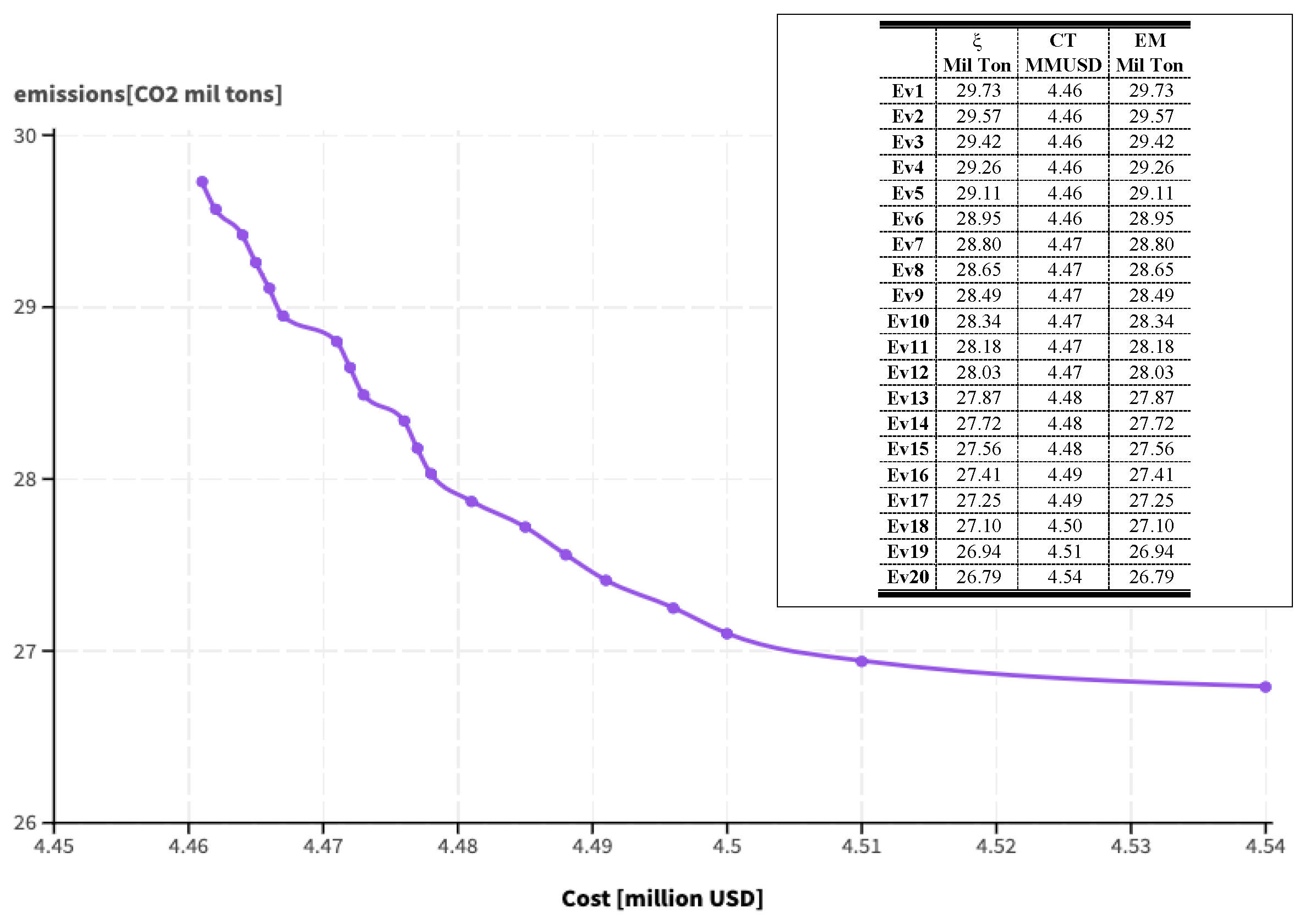
In this study, we use the multiobjective optimization model and the ξ -constraint method. For this effect, we establish 20 events. For each event, we solve a multiobjective optimization problem, obtaining the values of the objective functions, which will determine the Pareto front. Therefore, once the 20 events are solved, their results are shown in Figure 27.
With the Pareto front obtained, we apply the satisfaction methodology; in this sense, we proceed to find the membership functions or unitary functions, taking into account the maximum and minimum values obtained for each objective function, obtaining Table 13.
Here, we find the event that maximizes the minimum satisfaction between the two objective functions, whose result corresponds to the value of 0.737, which corresponds to event 15; in this context, this event is called the Pareto optimum. Therefore, we analyze the results obtained in event 15 (Pareto optimum). For event 15, we proceed to evaluate the generation dispatched and the exchanges between areas, which will allow us to know the energy production of the generating park of another area that will displace costly generation; for this reason, the dispatch carried out in each of the regions is shown in the following illustrations.
It also shows that we reduce the generation of area 1 most of the time compared to case 1 due to the supply of demand from interconnected regions. Additionally, compared to case 2, we observe an increase in generation during medium- and peak-demand periods and net values in the delivery or reception of energy concerning area 1. Table 14 presents these results. We observe that area 1 received 365.86 MWh during the analysis period, which aligns with the increase in production in this area compared to case 2, as is shown in Figure 28.
Likewise, the analysis concerns area 2, resulting in the economic office shown in Figure 29.
It also shows that, in the period of maximum demand, area 2 delivers from interconnected regions compared to case 2; Figure 30 shows the energy exchange, and it shows that the net between the energy received and delivered corresponds to a lower value of energy received than in case 2. Table 15 shows the details of this.
The analysis of area 3 is carried out similarly, resulting in the economic office shown in Figure 31.
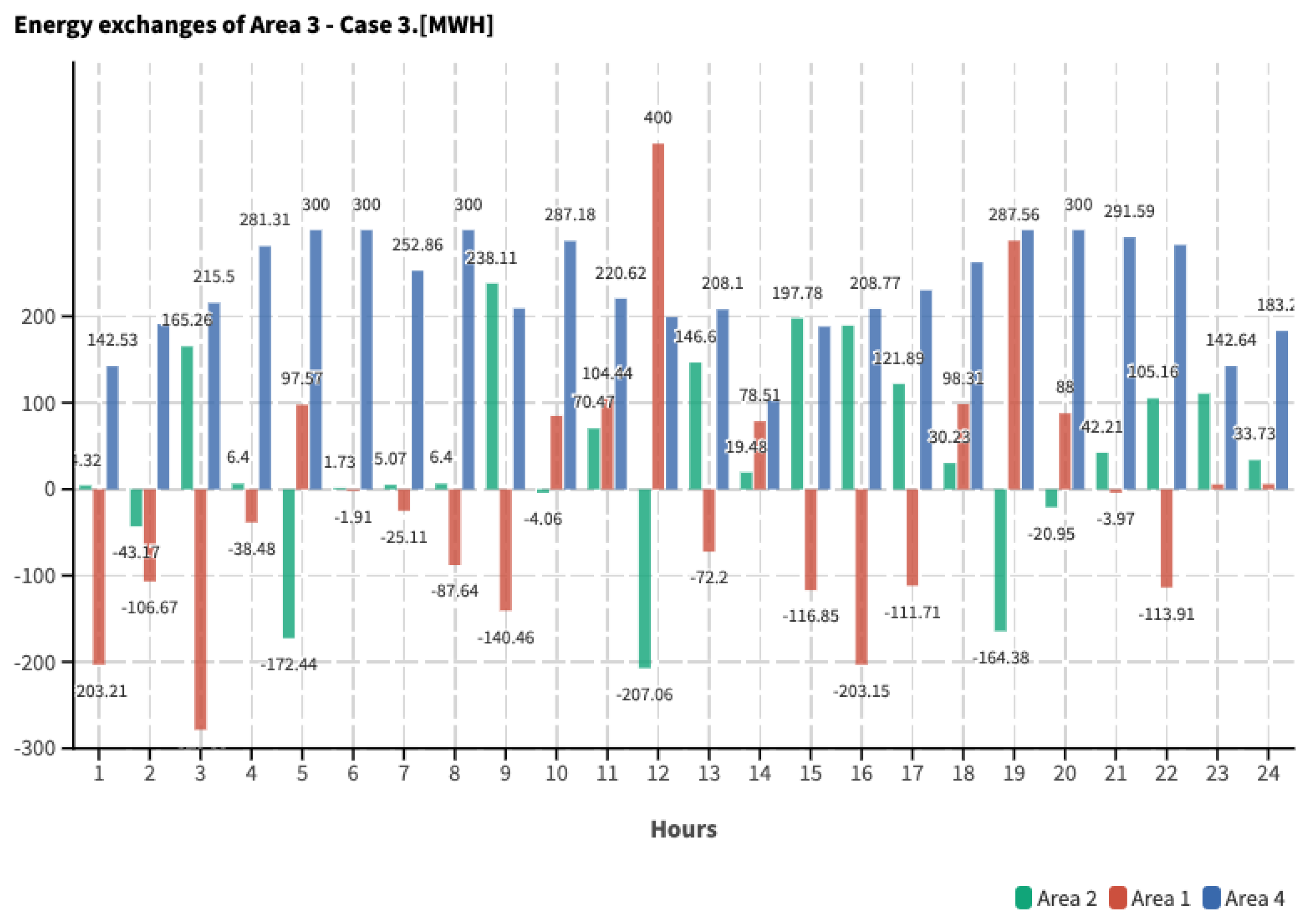
It also shows that this area continues to be the one that exports most of the energy to the four areas since most of the energy produced corresponds to economic energy; to establish the energy exchanges to the other areas, their values are described in Figure 32.
Table 16 shows that although area 3 receives energy occasionally, during most of the analysis period, it delivers energy mainly to area 4; the net value between energy received and delivered corresponds to a value of energy delivered. Although it is a little lower compared to case 2, the delivery of energy from this area to the other areas continues to predominate.
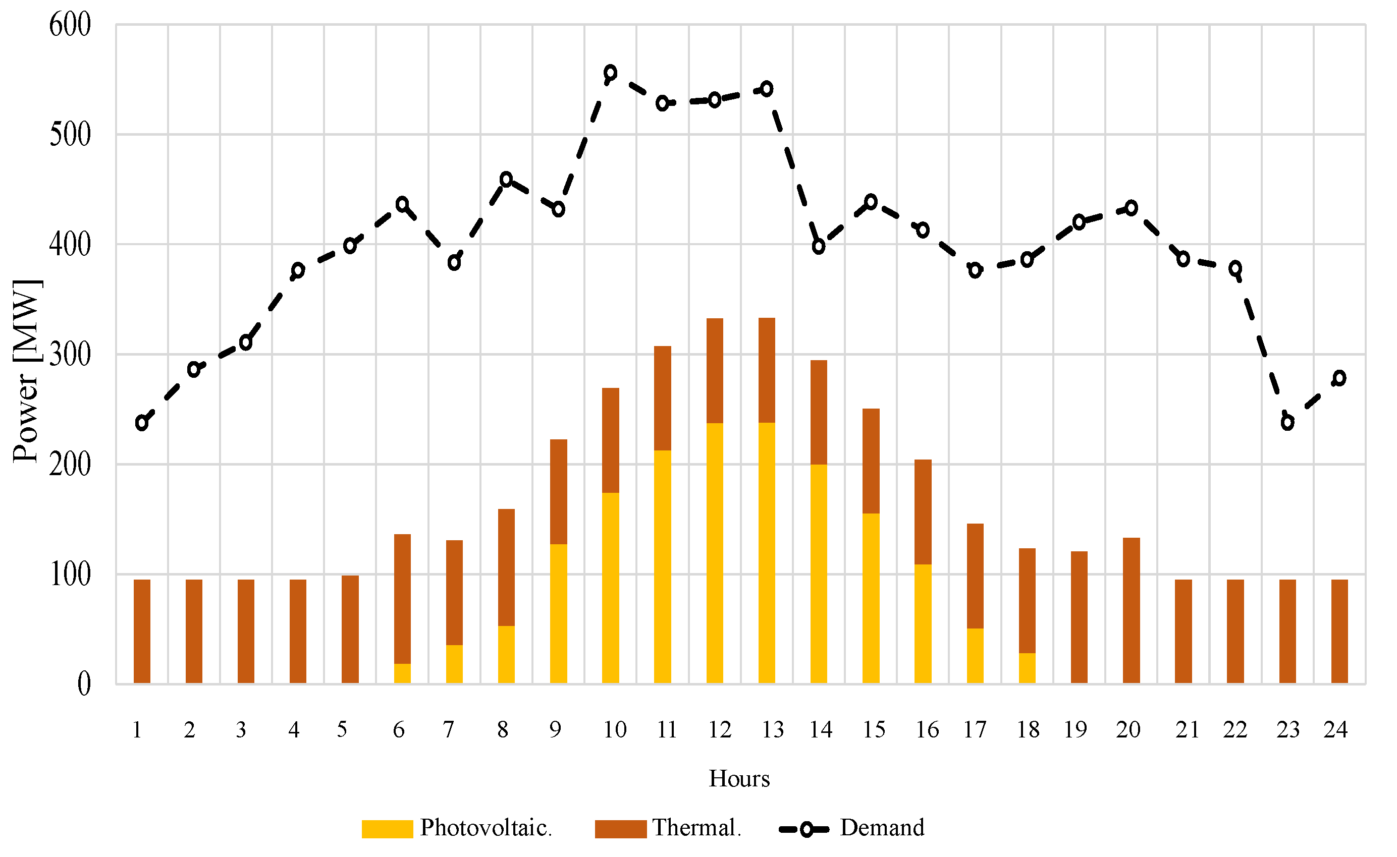
The analysis of area 4 is carried out similarly, resulting in the economic dispatch shown in Figure 33, and it shows that this area continues to receive most of the energy from area 3 since most of the energy produced and received by this area corresponds to economic energy; to establish the energy exchanges with the other areas, their values are described in Figure 34.
Here, it shows a significant import from area 3; the net value between energy received and delivered corresponds to the value of energy received, as shown in the Table 17.
After carrying out the individual analysis by area, it is necessary to illustrate the global supply in which the energy exchanges between areas are included, as shown in Figure 35.
It also shows that we effectively fulfill the multi-area and multi-objective dispatch, supplying the global demand. Next, Figure 36 displays the energy blocks by type of technology for each area.
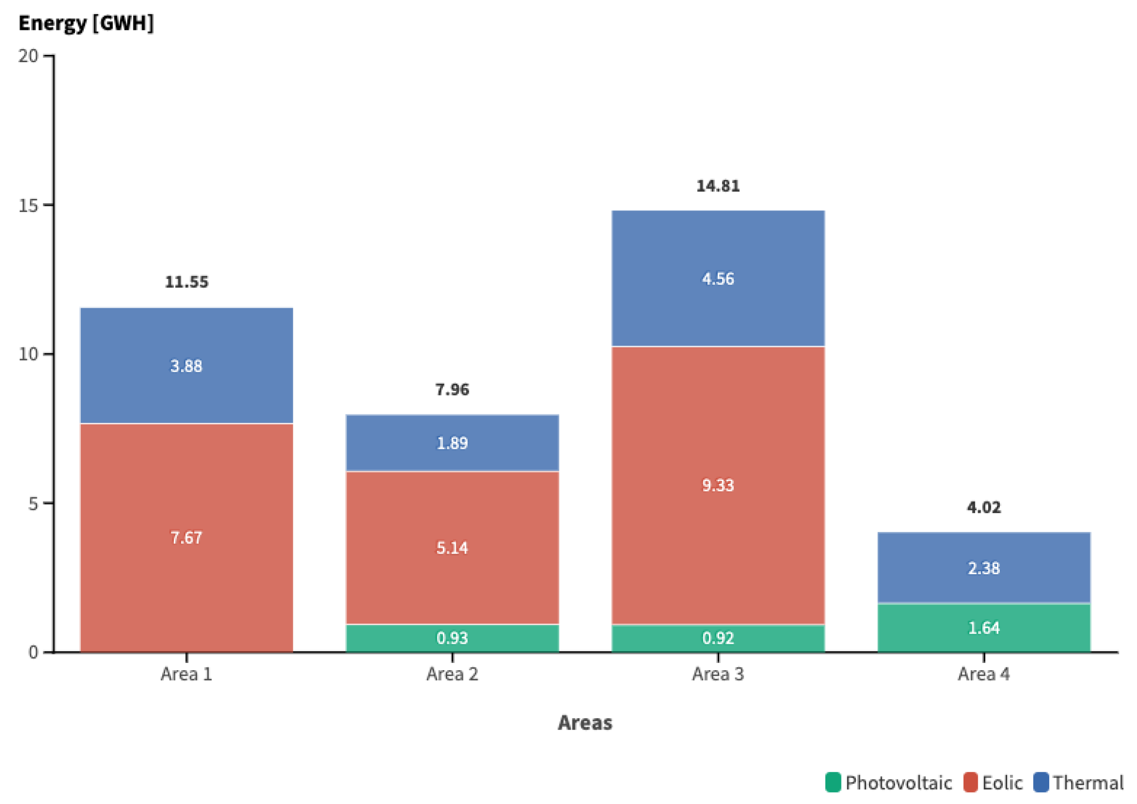
It also shows that, of the total energy, photovoltaic energy represents 9.1%, wind energy is equivalent to 57.7%, and energy from thermal generators amounts to 33.2%. From this, it can be concluded that the use of renewable energies is permanent, and its resource is taken advantage of; however, there is a reallocation of thermal production compared to case 2 to minimize CO 2 emissions. From the energy production resulting from the interconnected supply dispatch, we evaluate the economic values derived from the energy production associated with area and technology.
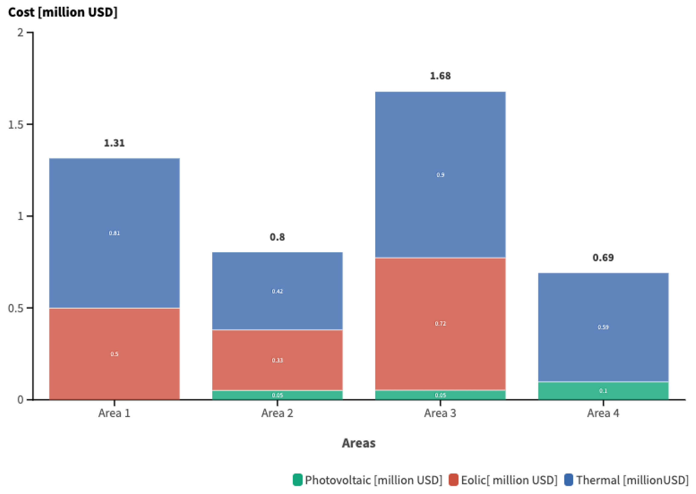
Figure 37 breaks down the total cost distribution among different energy generation technologies; thermal generation accounts for 61%, wind generation for 34.5%, and photovoltaic generation for 4.5%. This figure also illustrates the cost values by technology and area. Finally, we evaluate the amount of CO 2 emissions produced by thermal generators, and Figure 38 shows the results.
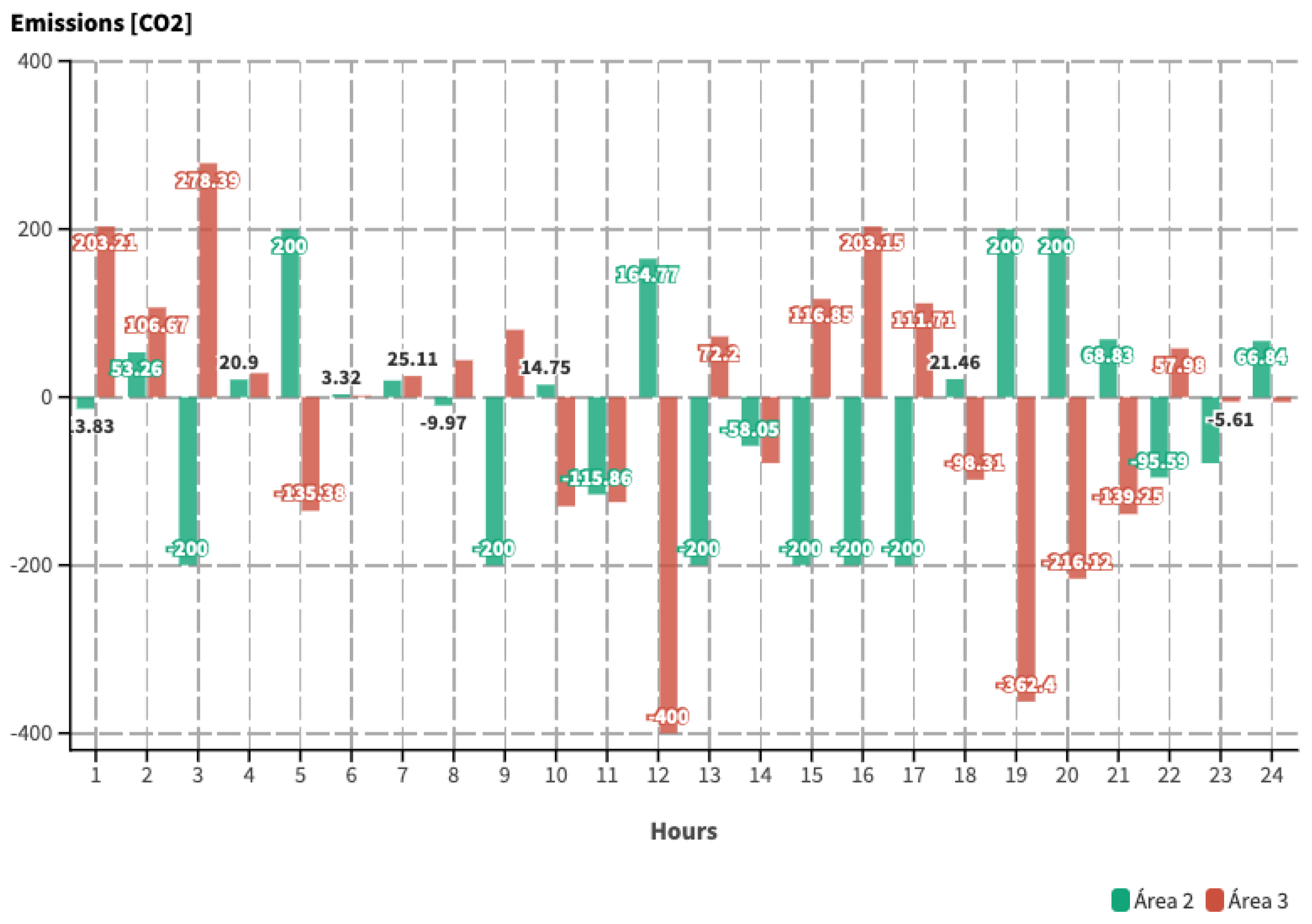
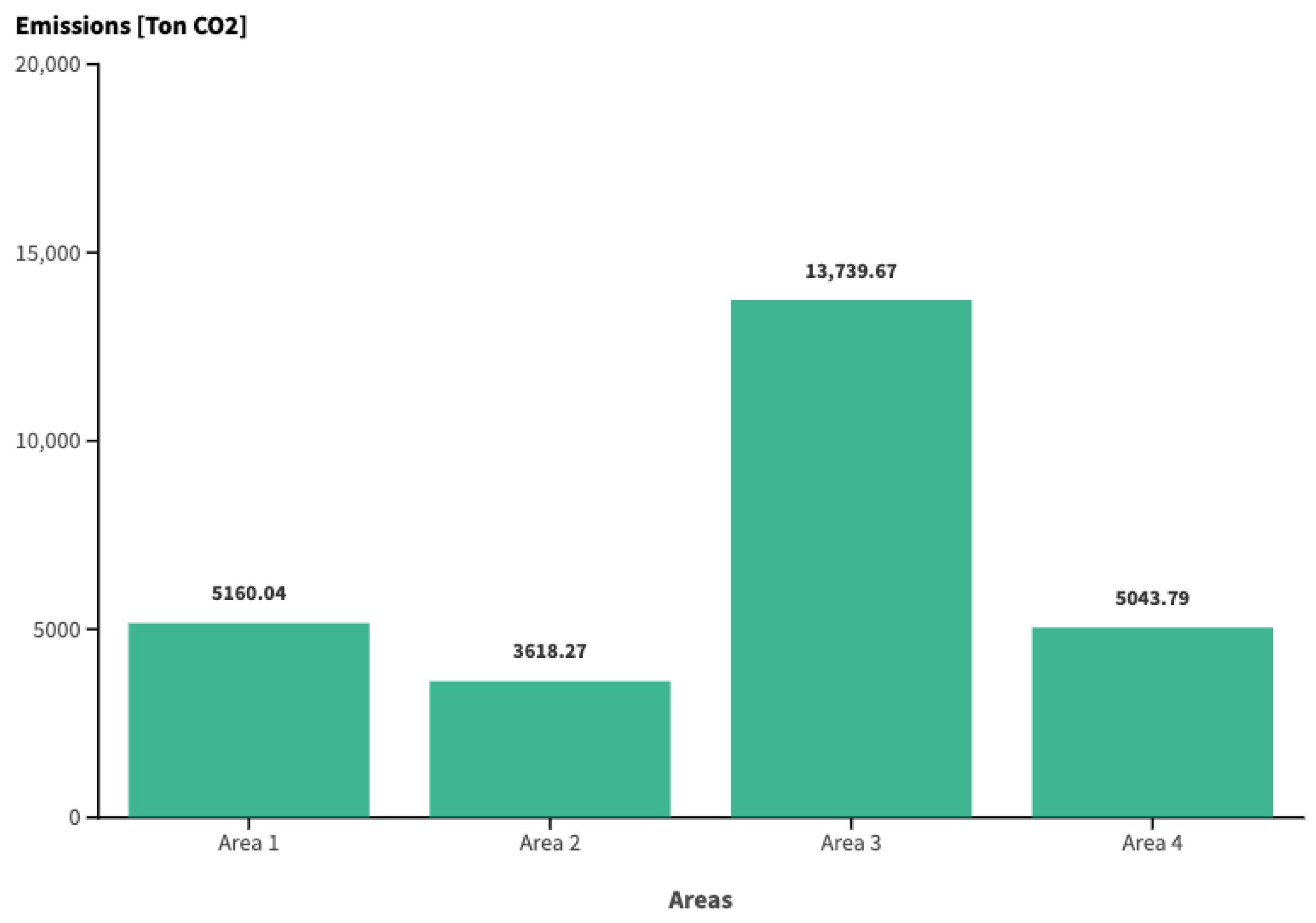
Compared to Study 2, there is a downward variation in CO 2 emissions, with a total value of 27,561.77 [tons] of CO 2 . A total of 50% of this value corresponds to emissions from area 3, while area 2 produces the minimum emissions, which amounts to 13%.

5.4. Comparative Analysis

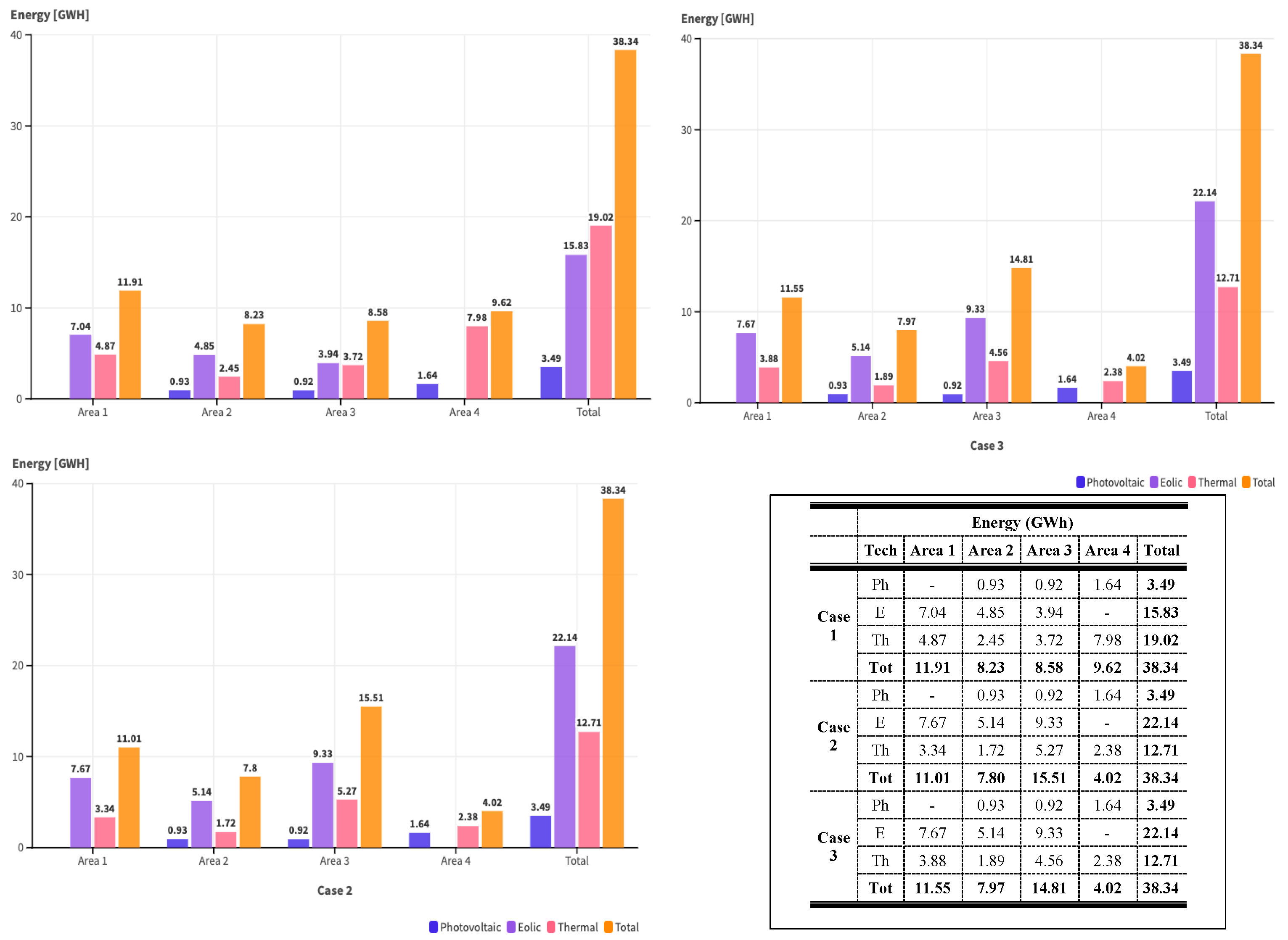
We conduct a comparative analysis of the economic and energy results evaluated in each study. First, we analyze the technical variables and show and tabulate the values in Figure 39.
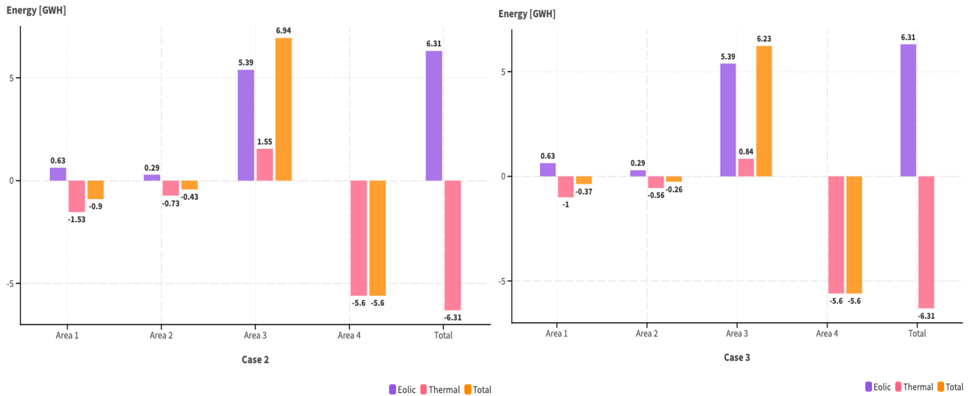
It also shows that the totals across any of the studies are identical because we need to supply the energy demand. However, significant variations in energy allocation occur depending on the study. To illustrate this, we show Figure 40, which highlights the variations in cases 2 and 3 compared to case 1.
It also shows that the totals in any of the studies are identical, given that it is required to supply the energy demand. However, depending on the study to be analyzed, there are significant variations in the energy allocation. For this purpose, Figure 40 is shown, which shows the variations in cases 2 and 3 concerning case 1. It can be observed that, regarding the variations in energy resulting from the photovoltaic power plants of cases 2 and 3 compared to case 1, there are significant variations, the most relevant being the one occurring in area 3, which delivers an incremental 5.39 GWH to the different areas. On the other hand, the energy production of the thermal power plants in studies 2 and 3 compared to study 1 varies substantially in all areas, which is appropriate given that the model optimizes the cost and energy of the most efficient plants. Of this area, four is considerably reduced by 5.6 GWH, which will implicitly guarantee a lower price globally. Figure 40 also shows significant energy variations in thermal generation between cases 2 and 3. This variation is not a random occurrence, but a deliberate action by the multi-objective model to comply with reducing CO 2 emissions. The model reallocates production to ensure compliance with its objectives, underlining the urgency and importance of our research in the field of energy allocation and optimization.
Furthermore, an economic analysis is conducted to assess the cost-effectiveness of the energy production obtained from the dispatch. The results, presented in Table 18, confirm the economic viability of the production process and show that study 1 is the most costly compared to the other two studies, which is correct given that the resources of all the areas are not optimized, which leads to a reduction in overall costs. This statement is shown by analyzing the prices obtained in studies 2 and 3, which generate cost savings in the study of USD 0.89 and 0.87 million, respectively. Case 2 shows the lowest cost of the cases analyzed, which is correct given that its result is consistent with the solved model that prioritizes cost minimization in a system that interconnects the areas. On the other hand, case 3 is USD 0.02 million more expensive than case 2, which is appropriate since the model in case 3 solves a multi-objective model where it satisfies the objective functions. Table 19 compares CO 2 emissions to observe the environmental impact.
In addition, it shows that case 1 has the highest value of CO 2 emissions, amounting to 40 thousand tons. However, by interconnecting the areas, overall emissions are reduced by 26% when comparing case 1 and case 2, generating a decrease of 10 thousand tons of CO 2 . Concerning case 3, the decrease is more significant, representing a 31% reduction compared to case 1, which corresponds to 12 thousand tons of CO 2 , which validates that the multi-objective model fulfills the purpose for which it was developed; in this sense, when comparing studies 2 and 3, the difference in the amount of emissions is 2 thousand tons of CO 2 which, when valued with the price of carbon credits according to [30] resulting in an income of approximately USD 170 thousand, which corresponds to extra income to the system, which in turn compensates for the slight increase in operating costs obtained in study 3.

6. Conclusions

The multi-objective optimization model that has been solved using non-linear programming and its result has allowed us to determine the hourly power to be dispatched by the generating park to minimize the costs associated with the operation of the system and the environmental impact.
The results related to the dispatch of the generation units located in the four different areas show that, when interconnecting them, the mathematical model optimizes the generation by observing the costs and capacity of the interconnection links. This optimization allows us to minimize costs and significantly reduce CO 2 emissions, a fact that we can all be proud of for its positive environmental impact.
As indicated in the previous conclusion, and considering the comparison of study 1 with studies 2 and 3, a substantial saving of approximately USD 900,000 is obtained in 24 h, corresponding to a value of roughly USD 325 million over the year. This aspect validates that the model reduces cost and creates savings by optimizing the generation of resources in all areas.
In addition to the above, analyzing the resulting and exchanged energy amounts shows that the model guarantees the hourly demand. Furthermore, the system can save even more when the capacity of the links is increased, allowing the savings from interconnecting the areas to be reinvested in expanding the links’ capacity.
The results of study 3 indicate that the model adequately satisfies the objective functions. However, the cost in study 3 and study 2 increases by USD 200 thousand, which can be offset with income from the sale of carbon credits, recovering approximately USD 170 thousand. We also observed a reallocation in the office, ensuring the efficient use of energy resources.
This analysis reveals that the multi-objective model excels in optimizing energy exchange, in addition to meeting the proposed objective functions. This optimization applies to many energy types, including thermal and renewable energies, even those with uncertainty in the primary resource. The model’s versatility in handling such uncertainty is a testament to its robustness, instilling confidence in its capabilities.

Future Work

Based on the novel concepts introduced in this study, we can propose the following innovative studies: generation dispatch for economic greenhouse gas emissions using a grasshopper optimization algorithm; multi-area dynamic economic dispatch of power system incorporating pumped hydro storage; evolution of dispatch rules using genetic programming to solve multi-objective generation dispatch problems; economic and environmental effects of renewable energy priority dispatch considering fluctuating power output from coal-fired units; optimization of transmission system expansion based on incorporating phase shifters to maximize reliability.

Author Contributions

P.C. conceptualized the study, analyzed the data, and wrote the initial draft. L.T. analyzed the data, revised the draft, provided critical feedback and edited the manuscript. All authors have read and agreed to the published version of the manuscript.

Funding

This research received no external funding.

Data Availability Statement

The original contributions presented in the study are included in the article, further inquiries can be directed to the corresponding author.

Acknowledgments

This work was supported by Universidad Politécnica Salesiana and GIREI —Smart Grid Research Group.

Conflicts of Interest

The authors declare no conflicts of interest.

References

  1. Prostejovsky, A.M.; Brosinsky, C.; Heussen, K.; Westermann, D.; Kreusel, J.; Marinelli, M. The future role of human operators in highly automated electric power systems. Electr. Power Syst. Res. 2019, 175, 105883. [Google Scholar] [CrossRef]
  2. Tong, K.; Ramaswami, A.; Feiock, R. Environmentally sustainable transitions of US district energy systems: Perspectives from infrastructure operators/designers through the co-evolutionary lens. J. Clean. Prod. 2020, 268, 121894. [Google Scholar] [CrossRef]
  3. Finkelman, R.B.; Wolfe, A.; Hendryx, M.S. The future environmental and health impacts of coal. Energy Geosci. 2021, 2, 99–112. [Google Scholar] [CrossRef]
  4. Moustakas, K.; Loizidou, M.; Rehan, M.; Nizami, A. A review of recent developments in renewable and sustainable energy systems: Key challenges and future perspective. Renew. Sustain. Energy Rev. 2020, 119, 109418. [Google Scholar] [CrossRef]
  5. Wu, Y.; Chen, X.; Ma, J.; Wu, Y.; Liu, D.; Xie, W. System integration optimization for coal-fired power plant with CO2 capture by Na2CO3 dry sorbents. Energy 2020, 211, 118554. [Google Scholar] [CrossRef]
  6. Viviescas, C.; Lima, L.; Diuana, F.A.; Vasquez, E.; Ludovique, C.; Silva, G.N.; Huback, V.; Magalar, L.; Szklo, A.; Lucena, A.F.; et al. Contribution of Variable Renewable Energy to increase energy security in Latin America: Complementarity and climate change impacts on wind and solar resources. Renew. Sustain. Energy Rev. 2019, 113, 109232. [Google Scholar] [CrossRef]
  7. Wu, J.; Qiu, J.; Wang, X.; Ni, Y.; Han, X.; Dai, J.; Du, Z.; Xie, X. Study on Medium and Long-Term Generation Expansion Planning Method Considering the Requirements of Green Low-Carbon Development. In Proceedings of the 2018 IEEE PES Asia-Pacific Power and Energy Engineering Conference (APPEEC), Kota Kinabalu, Malaysia, 7–10 October 2018; pp. 689–694. [Google Scholar] [CrossRef]
  8. Chen, Y.; Hou, J.; Chen, J.; Zheng, X.; Chen, H.; Liang, Z. A Novel Approach for Multi-Area Power System Day-ahead Scheduling under Uncertainties. In Proceedings of the 2018 IEEE Power & Energy Society General Meeting (PESGM), Portland, OR, USA, 5–9 August 2018; pp. 1–5. [Google Scholar] [CrossRef]
  9. Narimani, H.; Razavi, S.E.; Azizivahed, A.; Naderi, E.; Fathi, M.; Ataei, M.H.; Narimani, M.R. A multi-objective framework for multi-area economic emission dispatch. Energy 2018, 154, 126–142. [Google Scholar] [CrossRef]
  10. Azizivahed, A.; Ghavidel, S.; Ghadi, M.J.; Li, L.; Zhang, J. Multi-area economic emission dispatch considering load uncertainty. In Proceedings of the 2017 20th International Conference on Electrical Machines and Systems (ICEMS), Sydney, Australia, 11–14 August 2017; pp. 1–6. [Google Scholar] [CrossRef]
  11. Collins, S.; Deane, J.; Ó Gallachóir, B. Adding value to EU energy policy analysis using a multi-model approach with an EU-28 electricity dispatch model. Energy 2017, 130, 433–447. [Google Scholar] [CrossRef]
  12. Morris, J.; Farrell, J.; Kheshgi, H.; Thomann, H.; Chen, H.; Paltsev, S.; Herzog, H. Representing the costs of low-carbon power generation in multi-region multi-sector energy-economic models. Int. J. Greenh. Gas Control 2019, 87, 170–187. [Google Scholar] [CrossRef]
  13. Basu, M. Multi-area dynamic economic emission dispatch of hydro-wind-thermal power system. Renew. Energy Focus 2019, 28, 11–35. [Google Scholar] [CrossRef]
  14. Cheng, F.; Yang, M.; Han, X.; Liang, J. Real-time dispatch based on effective steady-state security regions of power systems. In Proceedings of the 2014 IEEE PES General Meeting | Conference & Exposition, National Harbor, MD, USA, 27–31 July 2014; pp. 1–5. [Google Scholar] [CrossRef]
  15. Basu, M. Multi-region dynamic economic dispatch of solar–wind–hydro–thermal power system incorporating pumped hydro energy storage. Eng. Appl. Artif. Intell. 2019, 86, 182–196. [Google Scholar] [CrossRef]
  16. Solaun, K.; Cerdá, E. Climate change impacts on renewable energy generation. A review of quantitative projections. Renew. Sustain. Energy Rev. 2019, 116, 109415. [Google Scholar] [CrossRef]
  17. Lei, Y.; Wang, D.; Jia, H.; Chen, J.; Li, J.; Song, Y.; Li, J. Multi-objective stochastic expansion planning based on multi-dimensional correlation scenario generation method for regional integrated energy system integrated renewable energy. Appl. Energy 2020, 276, 115395. [Google Scholar] [CrossRef]
  18. Sakawa, M.; Kato, K. An interactive fuzzy satisficing method for multiobjective structured linear programs and its application. In Proceedings of the 1995 IEEE International Conference on Systems, Man and Cybernetics, Intelligent Systems for the 21st Century, Vancouver, BC, Canada, 22–25 October 1995; Volume 5, pp. 4045–4050. [Google Scholar] [CrossRef]
  19. Huang, Y.; Hou, W.; Huang, Y.; Li, J.; Li, Q.; Wang, D.; Zhang, Y. Multi-Objective Optimal Operation for Steam Power Scheduling Based on Economic and Exergetic Analysis. Energies 2020, 13, 1886. [Google Scholar] [CrossRef]
  20. Khanna, M.; Rao, N.D. Supply and Demand of Electricity in the Developing World. Annu. Rev. Resour. Econ. 2009, 1, 567–596. [Google Scholar] [CrossRef]
  21. Jiyun, J.; Hu, C. Supply and Demand Conflict in Supply Chain Based on Principal-Agent Theory. In Proceedings of the 2009 Second International Conference on Intelligent Computation Technology and Automation, Changsha, China, 10–11 October 2009; pp. 11–14. [Google Scholar] [CrossRef]
  22. Armendáriz, M.; Heleno, M.; Cardoso, G.; Mashayekh, S.; Stadler, M.; Nordström, L. Coordinated microgrid investment and planning process considering the system operator. Appl. Energy 2017, 200, 132–140. [Google Scholar] [CrossRef]
  23. Gaur, A.S.; Das, P.; Jain, A.; Bhakar, R.; Mathur, J. Long-term energy system planning considering short-term operational constraints. Energy Strategy Rev. 2019, 26, 100383. [Google Scholar] [CrossRef]
  24. Wyrwa, A.; Suwała, W.; Pluta, M.; Raczyński, M.; Zyśk, J.; Tokarski, S. A new approach for coupling the short- and long-term planning models to design a pathway to carbon neutrality in a coal-based power system. Energy 2022, 239, 122438. [Google Scholar] [CrossRef]
  25. Carrillo-Galvez, A.; Flores-Bazan, F.; Parra, E.L. An Analytical Approach to the Environmental/Economic Dispatch Problem. In Proceedings of the 2019 IEEE CHILEAN Conference on Electrical, Electronics Engineering, Information and Communication Technologies (CHILECON), Valparaiso, Chile, 13–27 November 2019; pp. 1–5. [Google Scholar] [CrossRef]
  26. He, L.; Lu, Z.; Zhang, J.; Geng, L.; Cai, Y.; Li, X. Economic dispatch of multi-area integrated electricity and natural gas systems considering emission and hourly spinning reserve constraints. Int. J. Electr. Power Energy Syst. 2021, 132, 107177. [Google Scholar] [CrossRef]
  27. Zhang, H.; Zhang, S.; Cheng, H.; Zhang, C. Joint Generation, Transmission and Energy Storage Systems Expansion Planning in Multi-area Power Systems Considering Detailed Modeling of Tie lines. In Proceedings of the 2020 IEEE/IAS Industrial and Commercial Power System Asia (I&CPS Asia), Weihai, China, 13–16 July 2020; pp. 720–726. [Google Scholar] [CrossRef]
  28. Wang, X.; Shi, X.; Zhang, H.; Wang, F. Multi-objective optimal dispatch of wind-integrated power system based on distributed energy storage. In Proceedings of the IECON 2017—43rd Annual Conference of the IEEE Industrial Electronics Society, Beijing, China, 29 October–1 November 2017; pp. 2788–2792. [Google Scholar] [CrossRef]
  29. Sakthivel, V.; Suman, M.; Sathya, P. Combined economic and emission power dispatch problems through multi-objective squirrel search algorithm. Appl. Soft Comput. 2021, 100, 106950. [Google Scholar] [CrossRef]
  30. Lombardi, P.; Schwabe, F. Sharing economy as a new business model for energy storage systems. Appl. Energy 2017, 188, 485–496. [Google Scholar] [CrossRef]
  31. Singhal, P.K.; Naresh, R.; Sharma, V.; N, G.K. Enhanced lambda iteration algorithm for the solution of large scale economic dispatch problem. In Proceedings of the International Conference on Recent Advances and Innovations in Engineering (ICRAIE-2014), Jaipur, India, 9–11 May 2014; pp. 1–6. [Google Scholar] [CrossRef]
  32. Gubin, P.Y.; Oboskalov, V.P.; Mahnitko, A.; Gavrilovs, A. An Investigation into the Effectiveness of the Differential Evolution Method for Optimal Generating Units Maintenance by EENS Criteria. In Proceedings of the 2020 IEEE 61th International Scientific Conference on Power and Electrical Engineering of Riga Technical University (RTUCON), Riga, Latvia, 5–7 November 2020; pp. 1–5. [Google Scholar] [CrossRef]
  33. Saw, B.K.; Bohre, A.K. Multi DG Planning with Impact of Mixed-Load Models using Intelligent Methodologies: BF-PSO, PSO and GA. In Proceedings of the 2023 IEEE 3rd International Conference on Smart Technologies for Power, Energy and Control (STPEC), Bhubaneswar, India, 10–13 December 2023; pp. 1–5. [Google Scholar] [CrossRef]
  34. del Ambiente, M. Factor de Emision de CO2 del Sistema Nacional Interconectado de Ecuador. 2024. Available online: https://www.recursosyenergia.gob.ec/wp-content/uploads/2023/08/wp-1692720103183.pdf (accessed on 10 June 2024).
  35. Ministerio de Energía y Recursos Naturales No Renovables. Plan Maestro de Electricidad. Available online: https://www.recursosyenergia.gob.ec/plan-maestro-de-electricidad/ (accessed on 21 June 2024).
  36. Melgar-Dominguez, O.D.; Pourakbari-Kasmaei, M.; Mantovani, J.R.S. Robust Short-Term Electrical Distribution Network Planning Considering Simultaneous Allocation of Renewable Energy Sources and Energy Storage Systems. In Robust Optimal Planning and Operation of Electrical Energy Systems; Mohammadi-Ivatloo, B., Nazari-Heris, M., Eds.; Springer International Publishing: Cham, Germany, 2019; pp. 145–175. [Google Scholar] [CrossRef]
  37. Zhu, J. Optimization of Power System Operation; Wiley: Hoboken, NJ, USA, 2015. [Google Scholar] [CrossRef]
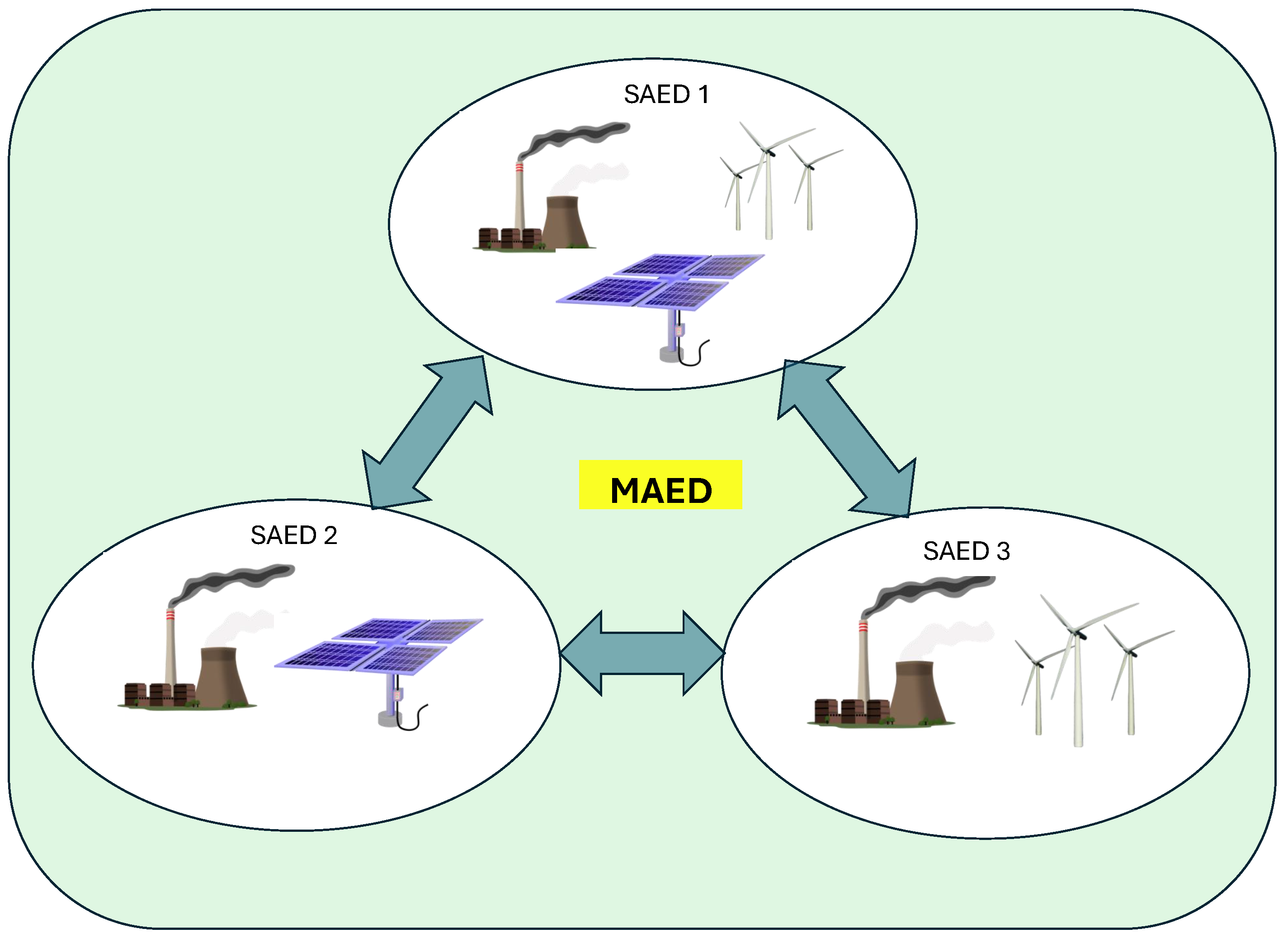
Figure 1. Multi-area economic dispatch.
Energies 17 05044 g001
Figure 2. Pareto front example.
Energies 17 05044 g002
Figure 3. Flowchart of the general multi-objective optimization model.
Energies 17 05044 g003
Figure 4. Scheme of interconnected areas.
Energies 17 05044 g004
Figure 5. Probability of wind resource use.
Energies 17 05044 g005
Figure 6. Probability of use of the photovoltaic resource.
Energies 17 05044 g006
Figure 7. Area demand.
Energies 17 05044 g007
Figure 8. Autonomous dispatch area 1.
Energies 17 05044 g008
Figure 9. Autonomous dispatch area 2.
Energies 17 05044 g009
Figure 10. Autonomous dispatch area 3.
Energies 17 05044 g010
Figure 11. Autonomous dispatch area 4.
Energies 17 05044 g011
Figure 12. Energy by technology and area—case 1.
Energies 17 05044 g012
Figure 13. Cost by technology and area—case 1.
Energies 17 05044 g013
Figure 14. Emissions [tons CO2].
Energies 17 05044 g014
Figure 15. Dispatch area 1—case 2.
Energies 17 05044 g015
Figure 16. Energy interchange area 1—case 2.
Energies 17 05044 g016
Figure 17. Dispatch area 2—case 2.
Energies 17 05044 g017
Figure 18. Energy interchange area 2—case 2.
Energies 17 05044 g018
Figure 19. Dispatch area 3—case 2.
Energies 17 05044 g019
Figure 20. Energy interchange area 3—case 2.
Energies 17 05044 g020
Figure 21. Energy dispatch area 4—case 2.
Energies 17 05044 g021
Figure 22. Energy interchange area 4—case 2.
Energies 17 05044 g022
Figure 23. Global sourcing dispatch—Case 2.
Energies 17 05044 g023
Figure 24. Energy by technology and area—case 2.
Energies 17 05044 g024
Figure 25. Cost by technology and area—case 2.
Energies 17 05044 g025
Figure 26. Emissions [ton CO2].
Energies 17 05044 g026
Figure 27. Pareto front—case 3.
Energies 17 05044 g027
Figure 28. Dispatch area 1—case 3.
Energies 17 05044 g028
Figure 29. Dispatch area 2—case 3.
Energies 17 05044 g029
Figure 30. Energy interchange area 2—case 3.
Energies 17 05044 g030
Figure 31. Dispatch area 3—case 3.
Energies 17 05044 g031
Figure 32. Energy exchange area 3—case 3.
Energies 17 05044 g032
Figure 33. Dispatch area 4—case 3.
Energies 17 05044 g033
Figure 34. Energy interchanges area 4—case 3.
Energies 17 05044 g034
Figure 35. Global sourcing dispatch—case 3.
Energies 17 05044 g035
Figure 36. Energy by technology and area.
Energies 17 05044 g036
Figure 37. Cost [millions USD] by technology and area.
Energies 17 05044 g037
Figure 38. Emissions [ CO 2 ]—case 3.
Energies 17 05044 g038
Figure 39. Comparison of energetic parameters.
Energies 17 05044 g039
Figure 40. Comparison of energetic parameters with energy variations.
Energies 17 05044 g040
Table 1. Pseudocode.
step 1set → Areas and load curves
 Demand periods
Data Area
Input → Technical Data generators
step 2Emissions CO 2 data
Productions cost
step 3Input → netting Data
Area interconnection
set F s , j , p , P g , s , p , C O T , E
Objetive function
C O T = C g t + C W + C R
step 4 C g t = s = 1 S p = 1 P g G A g , s P g , s , p 2 + B g , s P g , s , p + C g , s
C W = s = 1 S p = 1 P w W ϑ w , s P w , s , p
C R = s = 1 S p = 1 P r R μ r , s P r , s , p
Objetive Function 2:
E = s = 1 S p = 1 P g G d g , s P g , s , p 2 + e g , s P g , s , p + f g , s
Set → restrictions
step 5Model execute
step 6 ξ -constraint application
step 6execution of the fuzzy satisfaction method
step 7Optimum Pareto
step 8End
Table 2. Location and technology of the generating park.
NameTechnologyLocate
T1Thermal 
T2Thermal
T3ThermalArea 1
T4Thermal 
W1Eolic 
T5Thermal
T6Thermal
T7ThermalArea 2
W2Eolic 
FV1Photovoltaic 
T8Thermal
T9Thermal
T10Thermal
T11ThermalArea 3
W3Eolic 
W4Eolic 
FV2Photovoltaic 
T12Thermal
T13Thermal 
T14ThermalArea 4
T15Thermal 
FV3Photovoltaic 
Table 3. Parameters of the thermal generator park.
  P g min P g max E g T g
 [MW][MW][MW/h][MW/h]
T1201504545
T2351409090
T330230100100
T430350110110
T5101303535
T6202507070
T735250100100
T8301005050
T9602007575
T10251005555
T1140250100100
T12101305555
T1320250100100
T14352008080
T15301005050
Table 4. Coefficients of the cost function of the thermal power generation park.
  A g B g C g
 [USD/MWh2][cts/kWh][USD]
T10.0051916.554557.43
T20.0073221.078444.92
T30.0064822.140436.86
T40.0039820.009887.62
T50.0090821.536661.56
T60.0086018.708435.30
T70.0060220.113972.88
T80.0045922.195610.92
T90.0037219.883578.02
T100.0020115.775480.31
T110.0053517.074574.94
T120.0078422.590476.83
T130.0069523.728468.20
T140.0042721.444951.29
T150.0094422.378687.41
Table 5. Energy coefficients of the emission function of the thermal generating park.
  F 1 g F 2 g F 3 g
 MBTU/MWh2MBTU/kWhMBTU
T10.00436.120421.83
T20.00216.778220.77
T30.00616.845132.12
T40.00446.948144.45
T50.00506.950158.85
T60.00317.033224.37
T70.00137.169192.42
T80.00128.221129.60
T90.01618.625157.59
T100.00029.19266.96
T110.00467.334152.48
T120.00537.336167.68
T130.00327.423236.84
T140.00147.567203.11
T150.00128.677136.80
Table 6. Conversion factor to determine emissions from the thermal generating park.
Item Y g Item Y g
lb/MBTUlb/MBTU
T11.577T84.133
T21.568T93.781
T32.860T104.627
T42.698T112.860
T52.328T122.698
T62.622T132.328
T72.964T142.622
  T152.964
Table 7. Parameters of the generating park using renewable energies.
P nom Rate
[MW][cts/kWh]
W13806.5
W22706.4
W33007.3
W43308.2
FV11505.5
FV21805.7
FV31004.4
FV41407.1
Table 8. Interconnection link parameters.
LinkCapacity [MW]
Area 1–Area 2200
Area 1–Area 3400
Area 2–Area 3600
Area 4–Area 3300
Table 9. Net exchange of the area 1—case 2.
 Area 2 [MWH]Area 3 [MWH]Total [MWH]
Delivery1033.891329.702363.58
Reception−1571.94−1696.43−3268.36
Netting−538.05−366.73−904.78
Table 10. Net exchange of the area 2—case 2.
 Area 2 [MWH]Area 3 [MWH]Total [MWH]
Delivery614.891571.942186.83
Reception−1585.33−1033.89−2619.22
Netting−970.44538.05−432.39
Table 11. Net exchange of the area 3—case 2.
 Area 1 [MWH]Area 2 [MWH]Area 4 [MWH]Total
Delivery1585.331696.435601.448883.20
Reception−614.89−1329.700.0−1944.59
Netting970.44366.735601.446938.61
Table 12. Net exchange of area 4—case 2.
 Area 4Total
Delivery0.000.00
Reception−5601.44−5601.44
Netting−5601.44−5601.44
Table 13. Unit functions—case 3.
Events g c g Em Min ( g c ; g Em )
Ev11.00000.0000.000
Ev20.99780.0530.053
Ev30.99450.1050.105
Ev40.98940.1580.158
Ev50.98420.2110.211
Ev60.97890.2630.263
Ev70.96820.3160.316
Ev80.95520.3680.368
Ev90.94180.4210.421
Ev100.91990.4740.474
Ev110.89400.5260.526
Ev120.86770.5790.579
Ev130.83610.6320.632
Ev140.80090.6840.684
Ev150.75870.7370.737
Ev160.69270.7890.693
Ev170.61280.8420.613
Ev180.52630.8950.526
Ev190.39180.9470.392
Ev20-1.0000.000
Table 14. Net exchange of the area 1—case 3.
 Area 2 [MWH]Area 3 [MWH]Total
Delivery893.741499.692393.42
Reception−1512.41−1246.87−2759.28
Netting−618.67252.81−365.86
Table 15. Net exchange of the area 2—case 3.
 Area 2 [MWH]Area 3 [MWH]Total
Delivery612.061512.412124.47
Reception−1494.77−893.74−2388.51
Netting−882.71618.67−264.04
Table 16. Net exchange of the area 3—case 3.
 Area 1 [MWH]Area 2 [MWH]Area 4 [MWH]Total
Delivery1494.771246.875601.448343.09
Reception−612.06−1499.690.0−2111.75
Netting882.71−252.815601.446231.35
Table 17. Net exchange of area 4—case 3.
 Area 4Total
Delivery0.000.00
Reception−5601.44−5601.44
Netting−5601.44−5601.44
Table 18. Comparison of economic parameters [millions USD].
CaseAreasPhotovoltaicEolicThermalTotal
Area 1-0.4580.9881.446
Case 1Area 20.0510.3100.5280.890
Area 30.0520.2890.7591.101
Total0.2001.0574.0975.354
Area 1-0.4990.7121.211
Area 20.0510.3290.3910.772
Case 2Area 30.0520.7211.0171.790
Area 40.097-0.5930.690
Total0.2001.5492.7144.463
Area 1-0.4990.8151.314
Area 20.0510.3290.4230.803
Case 3Area 30.0520.7210.9041.677
Area 40.097-0.5930.690
Total0.2001.5492.7354.485
Table 19. Emissions comparison [tons CO 2 ].
AreaCase 1Case 2Case 3
Area 16711.354692.985160.04
Area 24721.483379.073618.27
Area 311,730.9916,612.6713,739.67
Area 416,850.795043.795043.79
Total40,014.6029,728.5027,561.77
Disclaimer/Publisher’s Note: The statements, opinions and data contained in all publications are solely those of the individual author(s) and contributor(s) and not of MDPI and/or the editor(s). MDPI and/or the editor(s) disclaim responsibility for any injury to people or property resulting from any ideas, methods, instructions or products referred to in the content.