Skip Content
You are currently on the new version of our website. Access the old version .
EnergiesEnergies
  • Article
  • Open Access

11 October 2024

Long-Term Forecasting Models of Oil Demand Emerging from the Global Petrochemical Sector

and
1
KAPSARC—King Abdullah Petroleum Studies and Research Center, Riyadh 11672, Saudi Arabia
2
Department of Economics, University of Perugia, 06123 Perugia, Italy
*
Authors to whom correspondence should be addressed.
This article belongs to the Special Issue Modeling Energy–Environment–Economy Interrelations II

Abstract

In the global energy mix by 2040, the growth in demand for oil and gas will be predominantly driven by the petrochemical sector across all regions of the world. The strong performance of this industry is anticipated to necessitate additional volumes of key feedstocks. Therefore, understanding the demand dynamics within the petrochemical sector is crucial for policy makers and industry stakeholders to make informed decisions regarding economic diversification, economic planning, and environmental sustainability. However, there is a notable lack of existing literature that explicitly addresses comprehensive regional and product-level demand modeling for petrochemical feedstocks. In this context, this study aims to estimate the demand for four main petrochemical feedstocks (Naphtha, Ethane, Liquefied Petroleum Gas (LPG), and other petrochemical feedstocks) across eight regions of the world. By estimating a total of 30 equations for price and income elasticities of demand in both the short and long term, the study provides detailed insights into the factors driving demand across different regions. The results demonstrate the robustness of the model, with good econometric properties and significant coefficients. In-sample regional simulations revealed small percentage errors across all regional equations, highlighting the model’s accuracy in tracking historical data. For each of the four feedstocks, an aggregate world equation—in other words, one single econometric world equation for each of the four petrochemical feedstocks’ categories mentioned earlier—was also estimated and compared against the aggregation of the regional simulations, with the latter found to track the history of global petrochemical feedstock demand better in-sample than a single econometric world equation. Overall, the study offers valuable contributions to the existing literature by filling a gap in comprehensive demand modeling for petrochemical feedstocks. It underscores the importance of regional and product-level analyses in understanding global demand patterns and informing strategic decisions in the industry.

1. Introduction

Some long-term forecast scenarios suggest that oil will continue to dominate the energy mix through 2050, primarily driven by demand in the transportation and petrochemical sectors [1,2,3]. Oil and gas combined are still expected to make up more than 50% of the global energy mix by 2040. Over the past decade, the petrochemical sector has seen significant growth in oil demand [4]. Demand growth from industry is driven mainly by the petrochemical sector, with its global demand forecast to increase by 3.7 million barrels per day (MMb/d) from 2021 to 2045 [3]. The strong performance of the petrochemical industry is expected to require additional volumes of natural gas as feedstock.
When examining patterns of petrochemical feedstock demand, we see different concentrations of petrochemical feedstock demand globally. According to Figure 1, and as reported by the IEA [5], naphtha is more in demand in Asia and Europe while ethane is more in demand in North America. Being a large exporter, the Middle East shows a balanced mix of ethane and naphtha demand.
Figure 1. Global petrochemical feedstock demand. Source: IEA [5]. Note: The left pie chart of each region indicates feedstock demand, while the right pie chart demonstrates primary chemical production.
However, it is anticipated by [4] that 2030 will see a slowdown of demand in emerging economies. They also surmise that this will eventually limit any intent to increase petrochemical plant capacities, inducing manufacturers to find solutions that will provide higher levels of productivity, especially in large-scale projects (e.g., [6]).
The importance of the petrochemical industry to overall industrial demand necessitates the construction of a long-term petrochemical demand model that forms part of a group of sectorial long-term oil demand models. These models should enable policy makers to understand the potential opportunities related to the demand for various oil products from different regions and sectors—the petrochemical sector being one of them. Indeed, such an understanding is crucial for oil-based economies, especially when experiencing adverse shocks from the oil market. Oil-based economies need to have a tool that enables them to foresee changes in oil demand to realize any opportunities and mitigate against potential challenges across all sectors (petrochemical, aviation, and maritime, among others). Non-oil-based economies and other entities can also benefit from such forecasting models. Furthermore, international agencies are likely to publish outlooks influenced by their member countries’ policies, making an independent long-term oil demand outlook useful.
However, forecasting sectoral oil demand presents several challenges due to the unique characteristics of each sector (e.g., [7]). Accurately predicting oil demand requires a deep understanding of these characteristics. To gain such insights, a set of seven models was planned, each focusing on one of the following sectors: aviation transport, maritime transport, land transport, the power sector, residential and commercial buildings, agriculture, and the petrochemical sector (e.g., [8]). This paper contributes to this objective by developing one of these models, specifically regional econometric demand models for oil demand in the global petrochemical sector.
In this paper, we present the methodology of the oil demand model for the petrochemical sector. The model is set at an annual frequency, with the estimation period running from 1970 to 2019.
The model is structured around four main products: naphtha, ethane, liquified petroleum gas (LPG), and other petrochemical feedstocks. It covers eight regions of the world: OECD Americas; OECD Europe; OECD Asia Oceania; Middle East and Africa; Latin America; Eurasia; Asia excluding China; and China. The first four represent industrialized regions, while the remaining regions represent a mix of emerging and developing economies, with the Middle East and Africa having a diverse range of development levels.
This paper is organized as follows. Section 2 presents the literature review of previous studies that have investigated the modeling of the petrochemical industry. Section 3 presents the detailed work of constructing the data bank of the petrochemical model and the estimation results. Section 4 shows the dynamic simulations in-sample. Section 5 presents the conclusion.

3. Data and Empirical Estimation

3.1. Data

The data bank for the petrochemical model was constructed using three main steps (see Appendix A for details). The first step in constructing the data bank of the petrochemical models is the construction of the quantity demanded for the four main dependent variables, namely naphtha, ethane, LPG, and other petrochemical feedstocks, all at the regional level.
The second step in constructing the data bank involves the construction of the macro variables at the regional level, which are used as a scale driver of the demand functions. The third step involves constructing the prices of the four products at the regional level. As referred to earlier, the general structure of the model comprises eight regions of the world: OECD Americas; OECD Europe; OECD Asia and Oceania; the Middle East and Africa; Latin America; Eurasia; Asia excluding China; and China. This gives a total of 32 elementary demand equations to be estimated and simulated. A further description of the above steps is presented in Appendix A.

3.2. Estimation

The theoretical foundation of the demand function is the optimization behavior theory, which specifies that the level of demand is a function of prices and income (e.g., [15]). We followed this approach, estimating a dynamic specification for each of the above regions and for each product. The demand variables are for ethane, naphtha, LPGs, and other petrochemical feedstocks. The price and income variables are assumed to be the main independent drivers. Given our aggregate approach to the demand function, we also considered some other exogenous variables to capture the specific regional and product characteristics of demand.
We model demand functions for eight regions and four feedstocks as a function of prices, gross domestic product (GDP), and other exogenous variables, with annual data for 1971–2019.
We cast a general ARDL model in log with lag = 1:
ln(Xij,t) = a0,ij + aij ln (pij,t) + bi Yi,t + Σk ci,k Zi,t,k + dij ln(Xij,t−1) + eij,t
where
j = naphtha, ethane, LPG, and other petrochemical feedstock products;
i = world, OECD Americas, OECD Asia Oceania, OECD Europe, Africa and Middle East, non-OECD Americas, non-OECD Europe and Eurasia, non-OECD Asia (excluding China), China (People’s Republic of China and Hong Kong, China);
Xij = quantity demand, by product and region;
pij = prices, by product and region;
Yi = GDP, by region;
Zi,k = other exogenous variables, by region i, where k = {population, GDP per capita, percentage of urban population}.
Note that in Equation (1), the main drivers for each sector’s oil demand are taken to represent changes and developments in economic growth, economic structure, population, and price.
For each equation, we performed a preliminary test for integration for all the variables in log, noting that there are both I(1) and I(0) series based on the significance of the Dicky–Fuller (DF) test. Therefore, we conducted a bound test ([16]) analysis for the four equations for the world, i.e., i = WORLD in Equation (1) for the purpose of comparison. The results in Table 1 confirm the existence of a long-run relationship among the quantity demand, price, and GDP for all variables, as the critical value of the upper bound of the F test at 5% is 4.35, thus allowing us to reject the null hypothesis of no long-run relationship.
Table 1. Bound test.
We estimated the demand equation for all products and regions. We performed robustness checks for each equation using four main tests: the Godfrey Breusch test for autocorrelation, given that there is a lag-dependent variable; the Jarque–Bera test for the normality of the residual; Ramsey’s RESET test for misspecification; and the Lagrange multiplier (LM) test for heteroskedasticity. For all equations, the robustness tests are non-significant, showing that there is no autocorrelation, the residuals are normal, there is no evidence of misspecification, and there is no evidence of heteroskedasticity.
The existence of a valid long-run relationship allows us to recover both the short-run and long-run price and income elasticities from the model of Equation (1). Since Equation (1) is expressed in a natural log format, the short-run elasticities are the estimated coefficients of the natural log of prices and income.
The long-run elasticity can be derived from the steady-state solution, i.e., when Xij,t = Xij,t−1.
The long-run equation is without time subscript:
ln(Xij) (1 − dij) = a0 + aij ln (pij) + bi Yi + Σk ci,k Zi,k
The long-run price and income elasticities are for every i, j, respectively:
Exij,pij = aij/(1 − dij) and Exij,Yi = bi/(1 − dij)

3.2.1. Ethane

The estimation results for ethane are reported in Table 2. The specification is adapted to the data for each region (dummy variables are not reported in the table).
Table 2. Ethane demand estimation.
The coefficients are all significant. The F-test for a joint coefficient is significant. The robustness tests show no autocorrelation, a normality of errors, an absence of heteroskedasticity, and an absence of misspecification (in the equation for the Middle East and Africa, the RESET test is mildly significant).
The short- and long-term elasticities of the demand for ethane are reported in Table 3. The price elasticities are generally inelastic, except for OECD Asia. The long-run elasticities are very high for the Middle East and Africa, and Asia. This shows the need for more investigation of the data and the estimation.
Table 3. Ethane demand elasticities.

3.2.2. Naphtha

The estimation results for naphtha are reported in Table 4. The specification is adapted to the data for each region (dummy variables are not reported in the table). The coefficients are all significant. The price variable for OECD Americas is one period lagged. The price variable for Asia is the log difference ([ln(p)-ln(p-1)]. The F-test for the joint coefficient is significant. The robustness tests show an absence of autocorrelation, a normality of errors, an absence of heteroskedasticity, and an absence of misspecification (in the equations for Latin America, the LM test is mildly significant). The short- and long-term elasticities of the demand for naphtha are reported in Table 5. The price is generally inelastic, except in Asia in the long run. The long-run elasticities are higher for the Middle East and Africa, and Eurasia.
Table 4. Naphtha demand estimation.
Table 5. Naphtha demand elasticities.

3.2.3. LPG

The estimation results for LPG are reported in Table 6. The specification is adapted to the data for each region (dummy variables are not reported in the table). The coefficients are all significant. The F-test for a joint coefficient is significant. The robustness tests show an absence of autocorrelation, a normality of errors, an absence of heteroskedasticity, and an absence of misspecification (in the equation for Latin America, normality and autocorrelation tests are significant). For OECD Asia, OCED Europe, and Latin America, the price term is the difference between the regional price and the world price.
Table 6. LPG demand estimation.
The short and long-term elasticities of LPG demand are reported in Table 7. The price elasticities are both elastic and inelastic. The long-run elasticities of price and income are very high for Asia.
Table 7. LPG demand elasticities.

3.2.4. Other Petrochemical Feedstocks

The estimation results for the demand for other petrochemical feedstocks are reported in Table 8. The specification is adapted to the data for each region (dummy variables are not reported in the table). The coefficients are all significant. The F-test for the joint coefficient is significant. The robustness tests show an absence of autocorrelation, a normality of errors, an absence of heteroskedasticity, and an absence of misspecification (in the equation for OECD Asia, the autocorrelation test is mildly significant).
Table 8. Other petrochemical feedstock demands estimation.
The short- and long-term elasticities of demand for other petrochemical feedstocks are reported in Table 9. The prices are generally inelastic, except in Eurasia and the Americas. The income elasticities are positive, except for OECD Americas, where the strong downward trend of the dependent variable results in negative income elasticity.
Table 9. Other petrochemical feedstock demand elasticities.

4. In-Sample Simulation

The equations have been dynamically simulated within the sample period. The common period of simulation is 1995–2019. We report, in Figure 2, the fitted values of the global equation for each product (the aggregated approach) and the sum of the fitted values of the regions’ equations for each product (the disaggregated approach). These results are reported to show the difference between the aggregated and disaggregated approach.
Figure 2. Simulation of actual and fitted values—world total—in-sample 1995 to 2019 (the vertical axis measures the quantity as MMb/d). Source: Authors.
In each panel of Figure 2, the right-hand graph depicts the difference between the sum of the fitted values of the regions’ equations for a given product and the sum of the actual observations of the same regions from the year 1995 to 2019 for a given product. However, the left-hand graph depicts the difference between the fitted values of the global equation for a given product and the sum of the actual observations of the regions for a given product. We report the historical values of the demand for naphtha, ethane, LPG, and other petrochemical products with the following respective variable labels: NT0, ET0, LT0, and OT0. We report the fitted values of the previously mentioned variables with the same labeling but with an ‘F’ prefix. For instance, ET0 is the sum of the actual observations for ethane demand across all regions’ products at time t; FET0 is the sum of the fitted values of the aggregate global equation for ethane at time t; FETW is the sum of the fitted values of the regions’ equations for ethane at time t.
Note that the sum of the disaggregated results seems to track the historical data better: FLTW is closer to the historical data than FLT0, and FOTW is closer to the historical data than FOT0. This is confirmed by the correlation shown in Table 10, where the first column shows the correlation between actual and fitted values for the aggregate equation, and the second column shows the correlation between actual and fitted values for the sum of the disaggregated regional equations. The correlation is similar for LPG and ethane, but it is higher for other petrochemical feedstocks and naphtha.
Table 10. Correlation coefficients—world historical vs. aggregate and disaggregated values.
The detailed simulations for each product for all regions are reported in Figure 3, Figure 4, Figure 5 and Figure 6. In each figure, the regions are identified with a numerical suffix: 1 = OECD Americas, 2 = OECD Asia, 3 = OECD Europe, 4 = Middle East and Africa, 5 = Latin America, 6 = Eurasia, 7 = Asia (other), 8 = China. In the case of ethane, we note the erratic pattern of historical data for region 6 and the lack of recent historical data for region 7. In both cases, the fitted values are smoother.
Figure 3. Simulation of actual and fitted values—ethane—regional values—in-sample 1995–2019 (the vertical axis measures the quantity as MMb/d). Source: Authors.
Figure 4. Simulation of actual and fitted values—naphtha—regional values—in-sample 1995–2019 (the vertical axis measures the quantity as MMb/d). Source: Authors.
Figure 5. Simulation of actual and fitted values—LPG—regional values—in-sample 1995–2019 (the vertical axis measures the quantity as MMb/d). Source: Authors.
Figure 6. Simulation of actual and fitted values—other petrochemical feedstocks—regional values—in-sample 1995–2019 (the vertical axis measures the quantity as MMb/d). Source: Authors.
The correlation coefficients and the root mean square errors of actual and historical data are reported in Table 11. Note that the correlation coefficients are generally high, with only a few exceptions. Note that the root mean square errors of the dynamic simulations are quite good, in the order of 1–3% for most equations, with only some values between 5% and 12% for naphtha and ethane in OECD Asia, OECD Europe, and Eurasia.
Table 11. Correlation coefficients and RMSE—regions’ historical vs. fitted values.

5. Conclusions

This paper has shown the methodology and results for a model that forecasts long-term regional demand for oil from the petrochemical sector. The general structure of the model comprises four main products: naphtha, ethane, LPG, and other petrochemical feedstocks for eight regions of the world: OECD Americas, OECD Europe, OECD Asia and Oceania, the Middle East and Africa, Latin America, Eurasia, Asia (excluding China), and China, for a total of 32 demand equations.
Due to the unavailability of demand data for certain feedstocks for two regions, we estimated 30 rather than 32 equations. We note that the results are quite satisfactory, with good econometric properties for all the equations estimated. We conducted significance tests, and all the coefficients are significant, so it is possible to estimate both price and income elasticities with the dynamic specification in the short and long term. We conducted the in-sample simulation of all the equations, finding that the percentage error of the simulation is satisfactorily small for all the equations. In particular, the dynamic simulations show a percentage error in the order of 1–3% for most equations, with only some values between 5% and 12% for naphtha and ethane in OECD Asia, OECD Europe, and Eurasia.
We also estimated an aggregate world equation and compared the results of that simulation with the results of the aggregation of the regional simulations. We find that the aggregation of the regional equations tracks the historical data in-sample better than a single econometric world equation. This indicates that disaggregating the analysis of demand into regional and product levels for petrochemical feedstocks facilitates valuable analysis.
The main contribution of this study is to provide a comprehensive model for estimating and potentially forecasting the demand for oil stemming from the petrochemical industry. In an era of significant changes driven by climate change mitigation efforts, decarbonization policies, and shifts in the global energy mix forecasted for the coming decades, it is crucial to focus on the main determinants of demand for petrochemical feedstocks. These feedstocks remain a crucial driver of oil and natural gas demand worldwide.
This study offers econometric estimations of price and income elasticities of petrochemical demand functions, which are valuable for both the oil and gas industry, as suppliers of feedstocks, and the petrochemical industry, as consumers of these feedstocks. Our methodology is beneficial for both industry stakeholders and policy makers worldwide, providing a better understanding of the non-energy use of hydrocarbons in the future. Additionally, this model serves as a valuable tool for future research, enabling the simulation of long-term forecasting scenarios.
Despite the robust results and significant findings presented in this study, we acknowledge that there may be some limitations that could stimulate future research. To address these limitations, extending the model to include other significant factors such as technological innovations, regulatory changes, and environmental considerations would provide a more comprehensive understanding of the sector. Furthermore, future studies could benefit from employing advanced econometric techniques or machine learning algorithms to enhance predictive accuracy and adapt to structural changes in the industry. Exploring the interactions between different sectors and their combined impact on petrochemical feedstock demand could also yield valuable insights.
Finally, as the global push for sustainability and carbon reduction intensifies, future research should incorporate scenarios that reflect potential shifts toward alternative energy sources and their impact on the petrochemical sector. Such future research would help policy makers and industry stakeholders better navigate the transition toward a more sustainable energy landscape.

Author Contributions

Conceptualization, R.A.M.; Methodology, R.A.M. and C.A.B.; Resources, R.A.M.; Data curation, R.A.M.; Writing—original draft, R.A.M.; Project administration, R.A.M. All authors have read and agreed to the published version of the manuscript.

Funding

This research received no external funding.

Data Availability Statement

The original contributions presented in the study are included in the article, further inquiries can be directed to the corresponding authors.

Conflicts of Interest

The authors declare no conflict of interest.

Appendix A

Methodology of the Data Bank Construction for the Petrochemical Demand Models.
The three main steps used to construct the data bank are described in detail below.
Step 1—Construction of the quantity demanded of the four main dependent variables
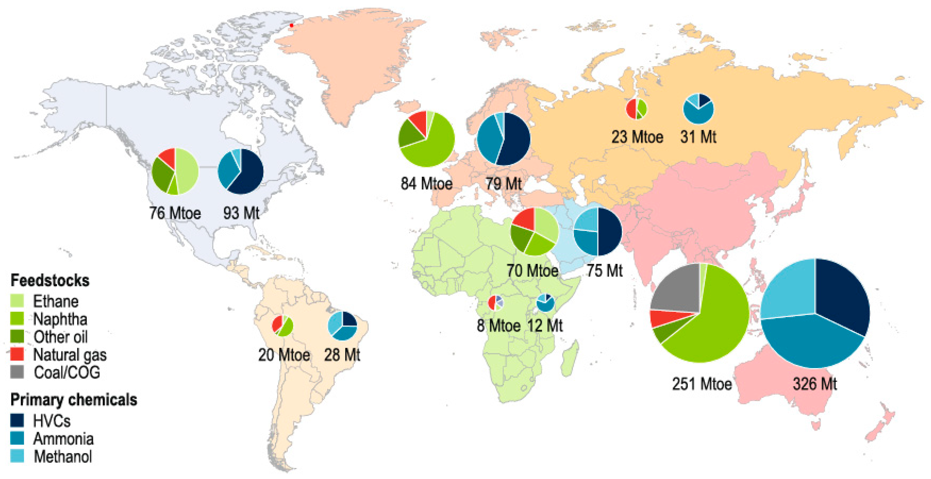
The data set is at the annual frequency and starts from 1971 until 2019. As mentioned, we aim to model the oil demand from different petrochemical feedstocks, namely naphtha, ethane, liquified petroleum gas (LPG), and other petrochemical feedstocks. To this end, we specify four dependent variables. These dependent variables measure the demand for petrochemical feedstocks for each region i. Therefore, the dependent variables are as follows:
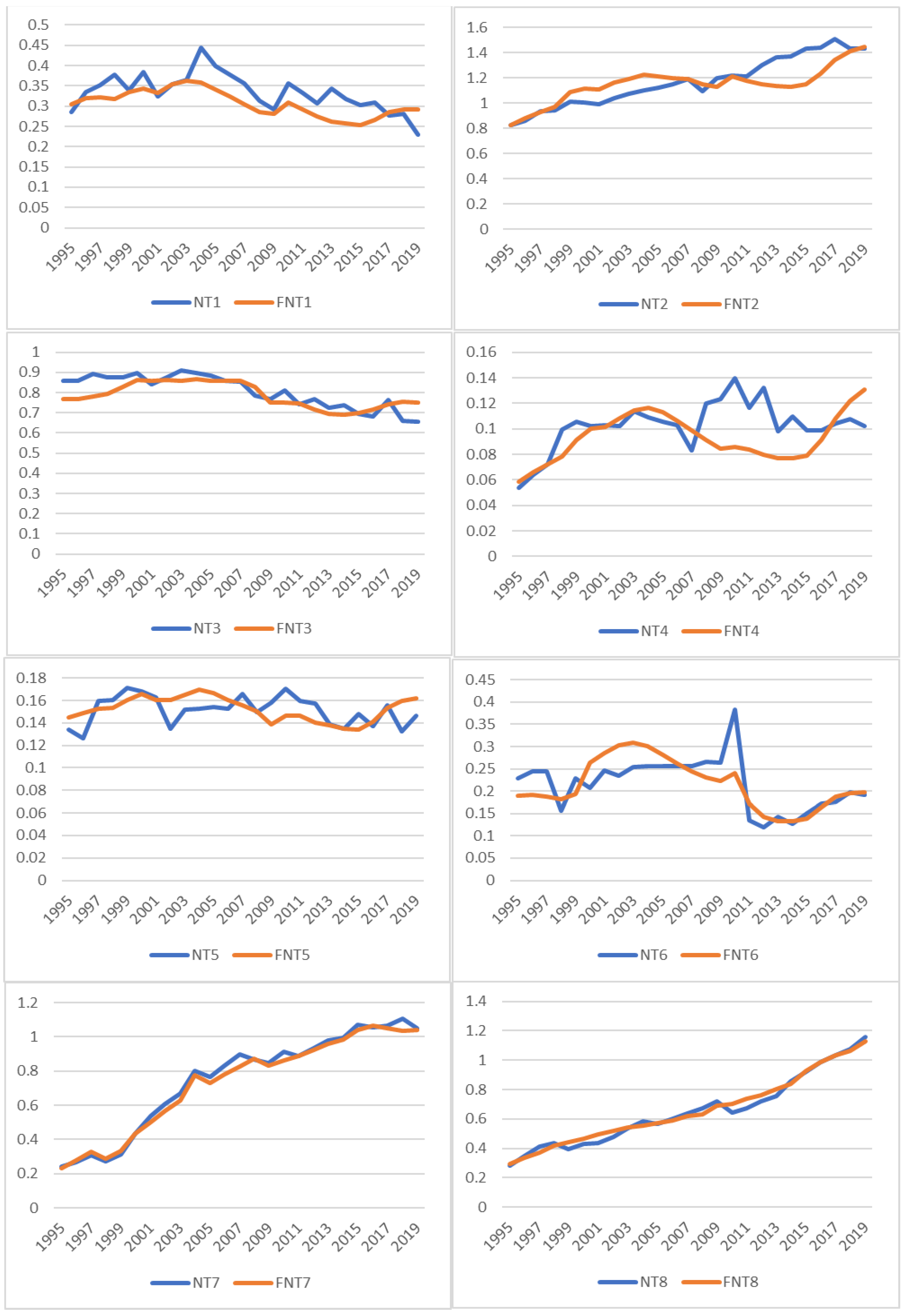
The demand for naphtha, denoted as NTi.
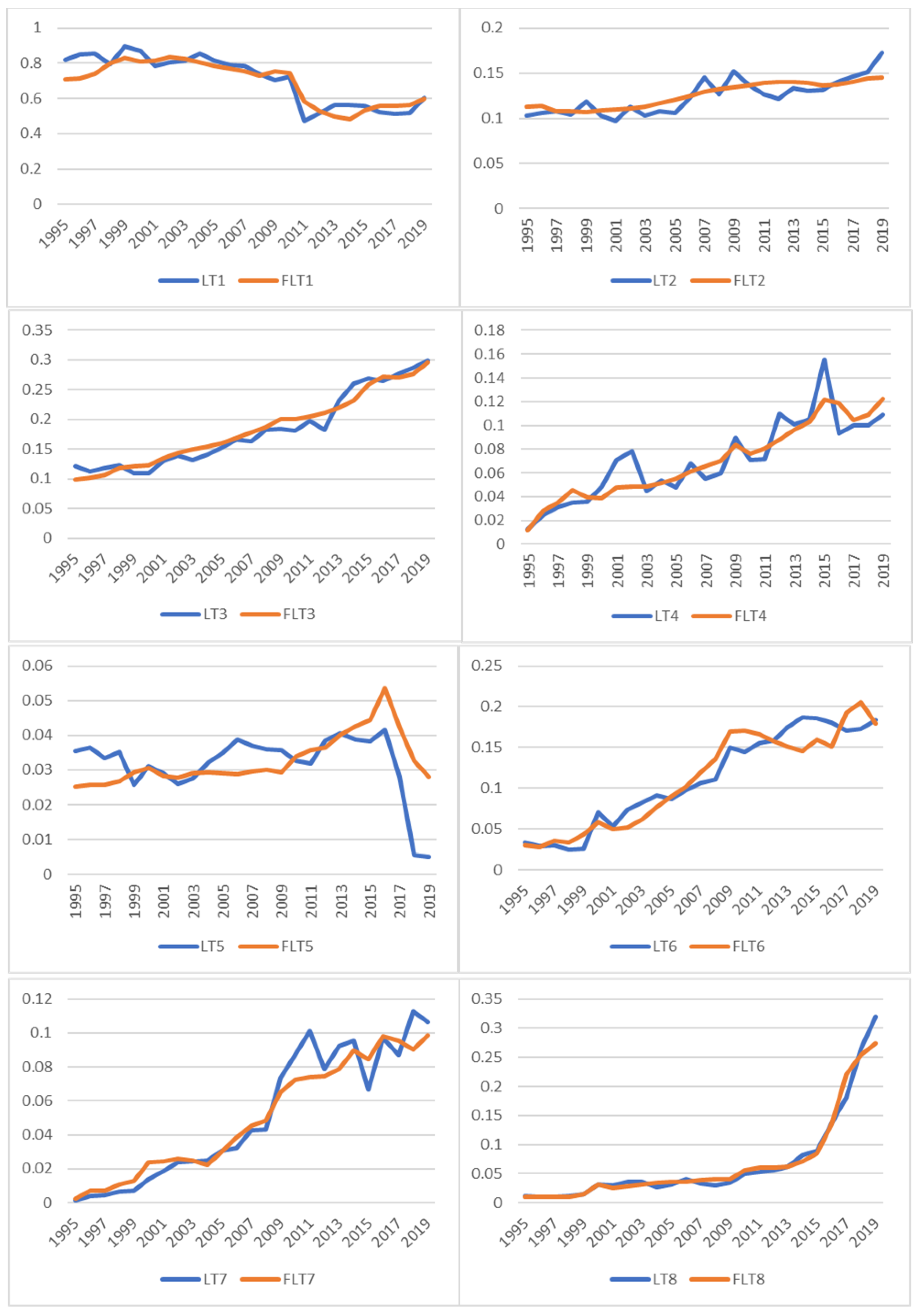
The demand for LPG, denoted as LTi.
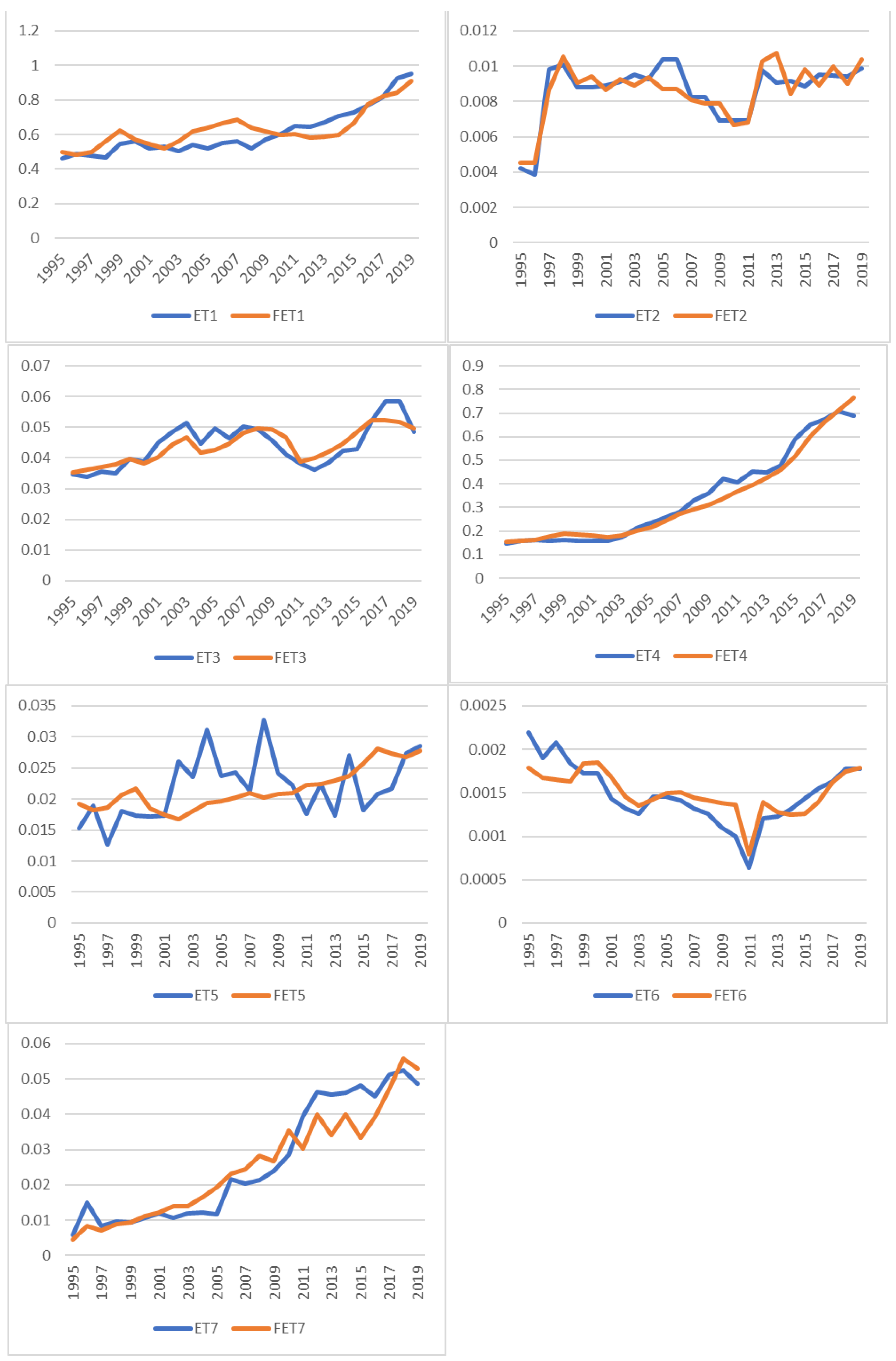
The demand for ethane, denoted as ETi.
Finally, the demand for other petrochemical feedstocks used in petrochemical plants is denoted as OTi.
All the demand is from petrochemical plants for the production of intermediate and final petrochemical products.
The aforementioned dependent variables are measured in our econometric models in million barrels of oil equivalent per day (MMboe/d). The reason for using this unit of measurement is to estimate the daily demand for oil from the petrochemical industry.
Furthermore, not only do we aim to forecast global demand, but we also estimated several regressions for each region of the world. Our estimation of demand has been developed for the following regions:
0-World
1-OECD America.
2-OECD Europe.
3-OECD Asia and Oceania.
4-Middle East and Africa.
5-Latin America.
6-Eurasia.
7-Asia, excluding China.
8-China.
The letter ‘i’ as a subscript to the previously mentioned variables (NTi, LTi, ETi, OTi) will be equal to 0, 1, 2, 3, 4, 5, 6, 7, and 8. Again, this means that there will be an estimated demand regression for each petrochemical feedstock for each ‘i’th region. The aforementioned dependent variables were collected from the International Energy Agency’s (IEA’s) World Energy Balances database, through a subscription [17,18], and measured in terms of kilotons of oil equivalent. The data set was converted from kilotons of oil equivalent to million barrels of oil equivalent per day by multiplying by 0.00714 and dividing by 365 days.
Step 2—Construction of the macroeconomic and socioeconomic explanatory variables
The second step involved the construction of the data set for the macroeconomic and socioeconomic variables, with data taken from the World Bank’s World Development Indicators [19] so as to have a homogeneous set of data. Data are at an annual frequency from 1971 to 2019 and were collected for the following variables:
Nominal gross domestic product (GDP) in United States (U.S.) dollars (USD).
Real GDP in USD (base = 2015).
Real GDP per capita.
Population in millions.
Percentage of population living in urban areas.
We have taken the data available at the country level for about 180 countries.
The aggregation is performed at the regional level, by summing GDP values in dollars, population in millions, and urban population in millions. We have taken the regional average GDP per capita by dividing GDP values by the population, and the percentage of the population living in urban areas is derived by dividing the urban population by the total population.
Step 3—Construction of the prices of the four dependent variables at the regional level
Step three involved the construction of the data set for the prices of the four petrochemical feedstocks (naphtha, ethane, LPG, and other petrochemical feedstocks), which were taken and assembled from two main sources, Platts and the United Nations Comtrade database [20]. From now on, we abbreviate this data source as UNCOMtrade. The Platts data are time series of prices expressed in USD per unit of measurement.
The UNCOMtrade data are a time series of exports and imports of values and quantities at the country level, from which it is possible to recover a measure of import and export unit values. These data have been used as a proxy for the price developments for certain time periods and regions missing in the Platts data. Accordingly, the data sources are as follows:
-
Platts Data Bank, considering prices of leading products in leading areas according to their classification (see Table A1).
-
UNCOMtrade United Nation Trade Data Bank, considering the SITC classification at the three- and four-digit level. Adapting this level of classification is essential for the purpose of capturing the exports, import values, and quantities of the four petrochemical feedstocks mentioned in this paper.
The SITC series taken as a proxy of the prices of the four products are the following:
Naphtha: proxy of price—product 3321, motor spirit, gasoline, and other light oils.
Ethane: proxy of price—product 271,111, natural gas, liquefied.
LPG: proxy of price—product proxy, product 3324, residual fuel oils.
Other oil: proxy of price—product proxy, product 3323, distillate fuels.
Data for the import and export unit values have been computed as dollar values divided by quantity for each product and each region.
The Platts price data are available for different regions and time periods. The elementary prices available from Platts are listed in Table A1. These data report prices for propane, butane, naphtha, gasoil, fuel oil, and gasoline for Asia, the Americas, Europe, and the Middle East. For some regions, different prices were reported.
Table A1. Platts price definitions.
Platts Code Name of Price Assessment Date AvailabilityRegionPetrochemical Feedstock
PMAAV00Propane Refrigerated CFR North Asia 30–60 days cargo 1982Asia Propane
PMAAF00Butane Refrigerated CF North Asia 30–60 DAYS CARGO1985Asia Butane
PAAAD00Naphtha c+f Japan Cargo USD/mt (NextGen MOC)1983Asia Naphtha
PAAAG00Naphtha c+f Japan Cargo 60–75 Days (NextGen MOC)1991Asia Naphtha
PAAAF00Naphtha c+f Japan Cargo 45–60 Days (NextGen MOC)1991Asia Naphtha
PAAAE00Naphtha c+f Japan Cargo 30–45 Days (NextGen MOC)1991Asia Naphtha
POABC00Gasoil FOB Spore Cargo1983Asia Gasoil
PUABE00FO 180 CST FOB ARAB GULF Cargo 1978Asia Fuel oil
PMAAT00Propane Conway Pipeline1983Americas Propane
PMAAD00Butane Conway spot1983Americas Butane
POAED00Gasoil No.2 USGC Prompt Pipeline1979Americas Gasoil
POAEE00Gasoil No.2 USGC Prompt waterborne1979Americas Gasoil
POAEG00Gasoil No.2 New York Harbor Barge1979Americas Gasoil
PUAFZ00USGC HSFO Waterborne (NextGen MOC)1979Americas Fuel oil
PAAAL00Naphtha CIF NEW Cargo USD/mt1990Europe Naphtha
PAAAM00Naphtha FOB Rdam Barge USD/mt1990Europe Naphtha
PMABA00Propane CIF NEW Large Cargo1985Europe Propane
PMAAS00Propane FOB ARA1985Europe Propane
PMAAK00Butane CIF NWE Large Cargo1985Europe Butane
PMAAC00Butane FOB ARA1985Europe Butane
PUAAL00FO 1% S CIF NEW Cargo1979Europe Fuel oil
PUAAP00FO 1% S FOB Rdam Barge1979Europe Fuel oil
PAAAI00naphtha FOB Med Cargo1979Africa Naphtha
PMABF00Propane FOB AG 20–40 DAYS CARGO vs. SAUDI PROPANE cp m11994MEPropane
PMABG00BUTANE FOB AG 20–40 DAYS CARGO vs. SAUDI BUTANE CP M11994MEButane
PAAAA00Naphtha FOB Arab Gulf Cargo1978MENaphtha
POAAT00Gasoil FOB Arab Gulf Cargo1983MEGasoil
PUABE00FO 180 CST FOB ARAB GULF Cargo 1978MEFuel oil
PUADV00FO 180 CST 3.5% S FOB SPORE CARGO1980Asia Fuel oil
PGACT00Gasoline Unl 87 USGC Prompt Pipeline1979U.S.Gasoline
Source: Platts. Note: ME = Middle East; FOB = free on board; USGC = U.S. Gulf Coast; CP = Contract Price; ARA = Amsterdam–Rotterdam–Antwerp; CIF = Cost, Insurance, and Freight; HSFO = High Sulfur Fuel Oil; MOC = Market on Close; FO = Fuel Oil; Rdam = Rotterdam; CFR = Cost and Freight; c+f = cost and fright; AG = Arabian Gulf; M1 = Month 1 (the next calendar month).
In Table A2, we associate the original Platts prices with the paper’s classification of regions.
The first crucial point to note is that Platts prices are available for different products for six regions of the world: Asia, the Americas, Europe, Africa, the Middle East, and the U.S. In Table A2, we show the correspondence between Platts’ and this paper’s regions. Platts data cover four main regions, and these have been attributed to the paper’s regional classifications. For instance, Platts’ Asia region corresponds to three regions of the paper’s classifications: OECD Asia, Asia excluding China, and China. Platts’ America region has been attributed to two of the paper’s regional classifications: OECD Americas and Latina America.
Table A2. Platts’ and this paper’s regional correspondence.
Platts’ RegionsThis Paper’s Regional Classifications
Asia2 OECD Asia7 Asia excl. China8 China
America1 OECD Americas5 Latin America
Europe3 OECD Europe6 Eurasia
Africa and ME4 Africa and Middle East
Source: Platts/Authors. Note: ME = Middle East; excl. = excluding.
The second point to note is that Platts’ product classification is different from this paper’s regional classification. Therefore, we used the Platts product prices for each region, as shown in Table A3. We used propane and butane for LT, naphtha for NT, gasoil, and fuel oil for OT. For instance, PMAAV00 and PMAAF00 are the prices that are used to construct a weighted average to proxy the price of LT for Asia.
Table A3. Definitions.
Prices
RegionLTNTOT
AsiaPMAAV00PAAAD00PUABE00
PMAAF00PAAAG00POABC00
PAAAF00
PAAAE00
AmericaPMAAT00PGACT00PUAFZ00
PMAAD00
EuropePMABA00 PUAAL00
PMAAS00 PUAAP00
PMAAK00
PMAAC00
ME and AfricaPMABF00PAAAI00POAAT00
PMABG00PAAAA00PUABE00
Source: Authors. Note: ME = Middle East; LT = Liquified Petroleum Gas (LPG); NT = Naphtha; OT = Other petrochemical feedstocks.
We then aggregated the prices for the countries, regions, and years available from the United Nations Comtrade database [20] according to our regional classification. We used a procedure with the function VLOOKUP to select the available data for the eight regions. This procedure is necessary because the data may contain a different number of reporting countries within each region for a given year. In other words, the data include varying numbers of countries for every year. The procedure avezzzyraged the country values for every year to obtain a time series with an average regional value for every year. Given the existing variability of the number of reporting countries in different years, with some reporting data on an intermittent basis, and some data clearly misreported, we decided to exclude the outlier countries from the yearly averages if the values deviate by more than one sigma from the regional average. Some of the misreported data were typically an underreporting of the quantity, which could give rise to excessive and implausible unit values (the division of a dollar value by a misreported quantity could result in a too high a unit value).
The data resulting from the above, for every region:
Time series with 52 observations 1971–2021 for naphtha ethane and LPG.
Time series with 39 observations 1971–2008 for other oil.
We then used the UNCOMTRADE unit values to estimate the missing data in the Platts data. Table A1 gives Platts data for different time periods. We averaged the UNCOMTRADE price indicators to match the Platts prices according to the correspondence shown in Table A2. Then we made a backward interpolation of the missing values for the Platts prices with the growth rates of the UNCOMTRADE price indicators for naphtha, LPG, and other petrochemical feedstocks. By doing this, we obtain a complete data set of Platts prices for the period 1971–2019. We used UNCOMTRADE data directly for ethane because Platts data do not report ethane prices.
The last phase was the construction of the time series for the four product prices for the eight regions used in the estimation. As explained above, we used the complete Platts data set to construct this paper’s regional prices, according to the correspondence shown in Table A2. We labeled the prices with the product suffix and the region suffix, as shown below:
PNT0 PNT1 PNT2 PNT3 PNT4 PNT5 PNT6 PNT7 PNT8
PET0 PET1 PET2 PET3 PET4 PET5 PET6 PET7 PET8
PLT0 PLT1 PLT2 PLT3 PLT4 PLT5 PLT6 PLT7 PLT8
POT0 POT1 POT2 POT3 POT4 POT5 POT6 POT7 POT8
For instance, PNT1 is the price of naphtha in region 1 (OECD Americas), PET2 is the price of ethane in region 2 (OECD Europe), and so on.

References

  1. OPEC. World Oil Outlook. 2019. Available online: https://www.opec.org/opec_web/static_files_project/media/downloads/publications/WOO_2019.pdf (accessed on 24 May 2024).
  2. OPEC. World Oil Outlook. 2020. Available online: https://www.opec.org/opec_web/static_files_project/media/downloads/publications/OPEC_WOO2020.pdf (accessed on 24 May 2024).
  3. OPEC. World Oil Outlook. 2022. Available online: https://www.opec.org/opec_web/static_files_project/media/downloads/WOO_2022.pdf (accessed on 24 May 2024).
  4. Cetinkaya, E.; Liu, N.; Simons, T.J.; Wallach, J. Petrochemicals 2030: Reinventing the Way to Win in a Changing Industry; Insight article; McKinsey & Company: Chicago, IL, USA, 2018. [Google Scholar]
  5. IEA World Energy Outlook. 2020. Available online: https://www.iea.org/reports/world-energy-outlook-2020 (accessed on 24 May 2024).
  6. Lange, J.-P. Towards circular carbo-chemicals-the metamorphosis of petrochemicals. Energy Environ. Sci. 2021, 14, 4358–4376. [Google Scholar] [CrossRef]
  7. Dehghanchaharabi, A. The Future of Petrochemicals: Towards More Sustainable Plastic and Fertilisers; International Energy Agency (IEA): Paris, France, 2018. [Google Scholar]
  8. OECD. Improving Plastics Management: Trends, Policy Responses, and the Role of International Co-Operation and Trade; Background report prepared for the G7 environment, energy and oceans ministers; OECD: Paris, France, 2018. [Google Scholar]
  9. Butterfield, D.W.; Kubursi, A.A.; Welland, J.D. A Model of the Petrochemical Industry. J. Energy Dev. 1983, 9, 299. [Google Scholar]
  10. Hasanov, E.; Hasanov, M. Analysing the Relationship Between Oil Prices and Basic Petrochemical Feedstocks. In Energy Economy, Finance and Geostrategy; Dorsman, A., Ediger, V., Cham, M.K., Eds.; Springer: Berlin/Heidelberg, Germany, 2018. [Google Scholar]
  11. Dahl, C. A Survey of Energy Demand Elasticities for the Developing World. J. Energy Dev. 1992, 18, 1. [Google Scholar]
  12. Liu, F.; Shao, S.; Zhang, C. How Do China’s Petrochemical Markets React to Oil Price Jumps? A Comparative Analysis of Stocks and Commodities. Energy Econ. 2020, 92, 104979. [Google Scholar] [CrossRef]
  13. Lyua, B.; Kwon, H.; Leeb, J.; Yoonb, H.; Jin, J.; Moon, I. Forecasting of Naphtha Demand and Supply Using Time Serial Data Causal Analysis. Comput. Aided Chem. Eng. 2014, 33, 829–834. [Google Scholar]
  14. Rao, R.D.; Parikh, J.K. Forecast and Analysis of Demand for Petroleum Products in India. Energy Policy 1996, 24, 583–592. [Google Scholar] [CrossRef]
  15. Pedregal, D.J.; Dejuán, O.; Gómez, N.; Tobarra, M.A. Modelling Demand For Crude Oil Products in Spain. Energy Policy 2009, 37, 4417–4427. [Google Scholar] [CrossRef]
  16. Pesaran, M.H.; Shin, Y.; Smith, R.J. Bounds Testing Approaches to the Analysis of Level Relationships. J. Appl. Econom. 2001, 16, 289–326. [Google Scholar] [CrossRef]
  17. IEA. World Energy Outlook. 2022. Available online: https://www.iea.org/reports/world-energy-outlook-2022 (accessed on 24 May 2024).
  18. United States Energy Information Administration (EIA). International Energy Outlook. 2021. Available online: https://www.eia.gov/outlooks/ieo/pdf/IEO2021_Narrative.pdf (accessed on 24 May 2024).
  19. World Bank. World Development Indicators (WDI). 2022. Available online: https://databank.worldbank.org/source/world-development-indicators (accessed on 25 May 2023).
  20. United Nations. UN Comtrade Database. 2023. Available online: https://comtradeplus.un.org/ (accessed on 1 April 2023).
Disclaimer/Publisher’s Note: The statements, opinions and data contained in all publications are solely those of the individual author(s) and contributor(s) and not of MDPI and/or the editor(s). MDPI and/or the editor(s) disclaim responsibility for any injury to people or property resulting from any ideas, methods, instructions or products referred to in the content.

Article Metrics

Citations

Article Access Statistics

Multiple requests from the same IP address are counted as one view.