
Multi-Objective Optimization Operation of Multi-Agent Active Distribution Network Based on Analytical Target Cascading Method

Abstract
1. Introduction
- (1)
- For the impact of distributed photovoltaic integration on distribution network operation, considering the operational constraints of various active management elements, a multi-objective optimization model for dynamic optimal power flow based on mixed-integer second-order cone programming (MISOCP) is established with the goal of minimizing reverse power flow, node voltage deviation, line active power loss, and photovoltaic curtailment penalties, achieving optimized scheduling for the distribution network.
- (2)
- For various flexible resources within the feeder area, a power aggregation and demand response model is established, constructing a mixed-integer linear programming (MILP) model with the objective of optimizing the economic efficiency and energy comfort of load aggregators, achieving optimal scheduling for the feeder area.
- (3)
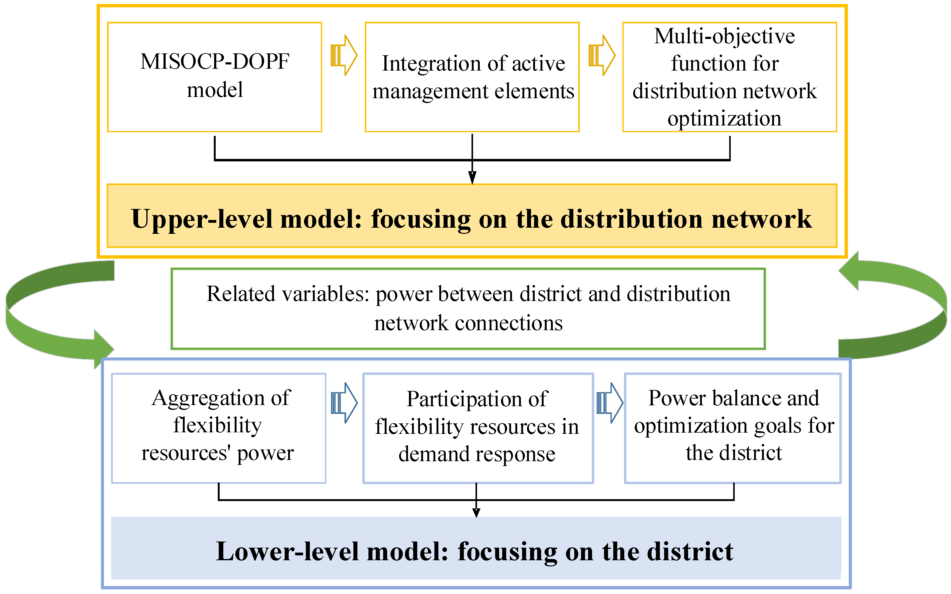
- A two-level hierarchical optimization scheduling model is established, with the MISOCP-DOPF model for the distribution network as the upper layer and the MILP model for the feeder area as the lower layer. The ATC method is used for model decoupling, achieving coordinated optimization of the distribution network and feeder area operations.
2. Active Distribution Network Modeling
2.1. Objective Function
2.2. Constraints
2.2.1. System Flow Constraints
2.2.2. OLTC Operating Constraints
2.2.3. CB and SVC Operating Constraints
2.2.4. Constraints for DG Operation
3. Modeling of Distribution Feeder Areas
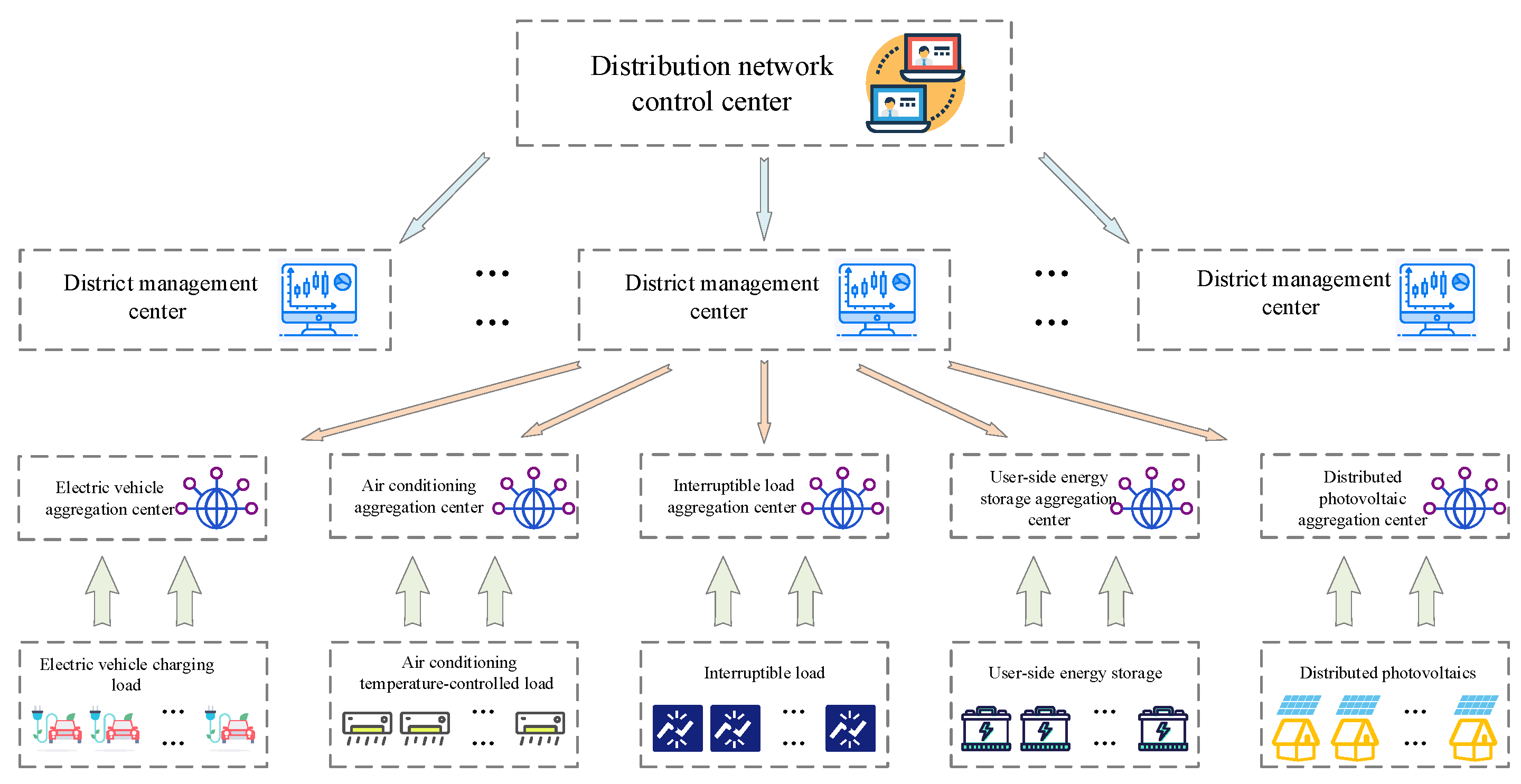
3.1. System Architecture
3.2. Objective Function
3.2.1. Economic Indicators
3.2.2. User Temperature Satisfaction Indicator
3.3. Constraints
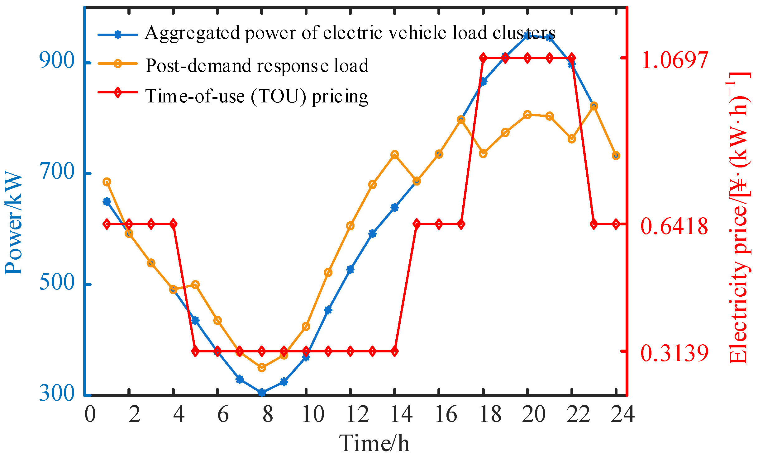
3.3.1. EV Constraints
3.3.2. Air Conditioning Constraints
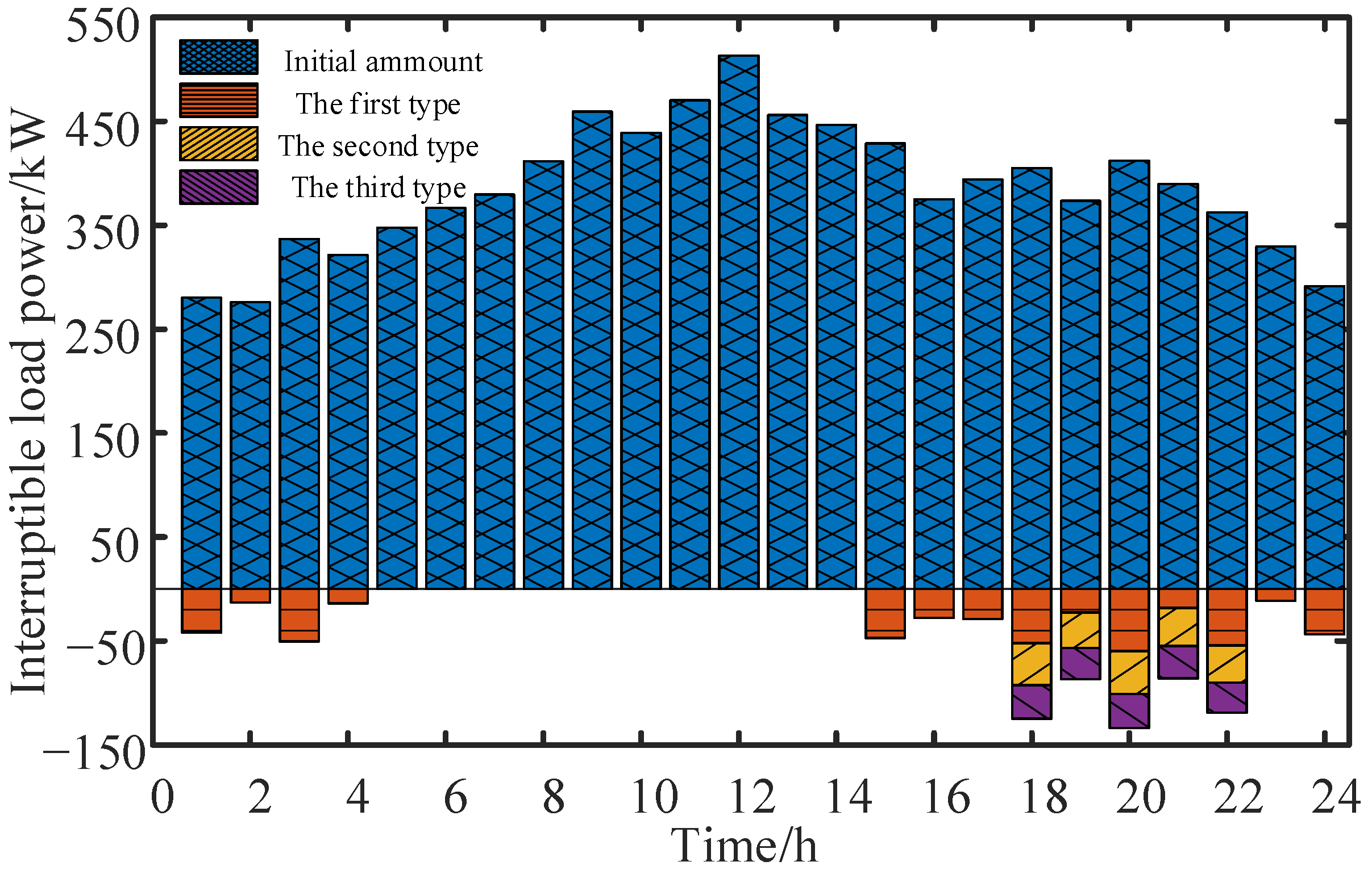
3.3.3. Constraints on Interruptible Loads
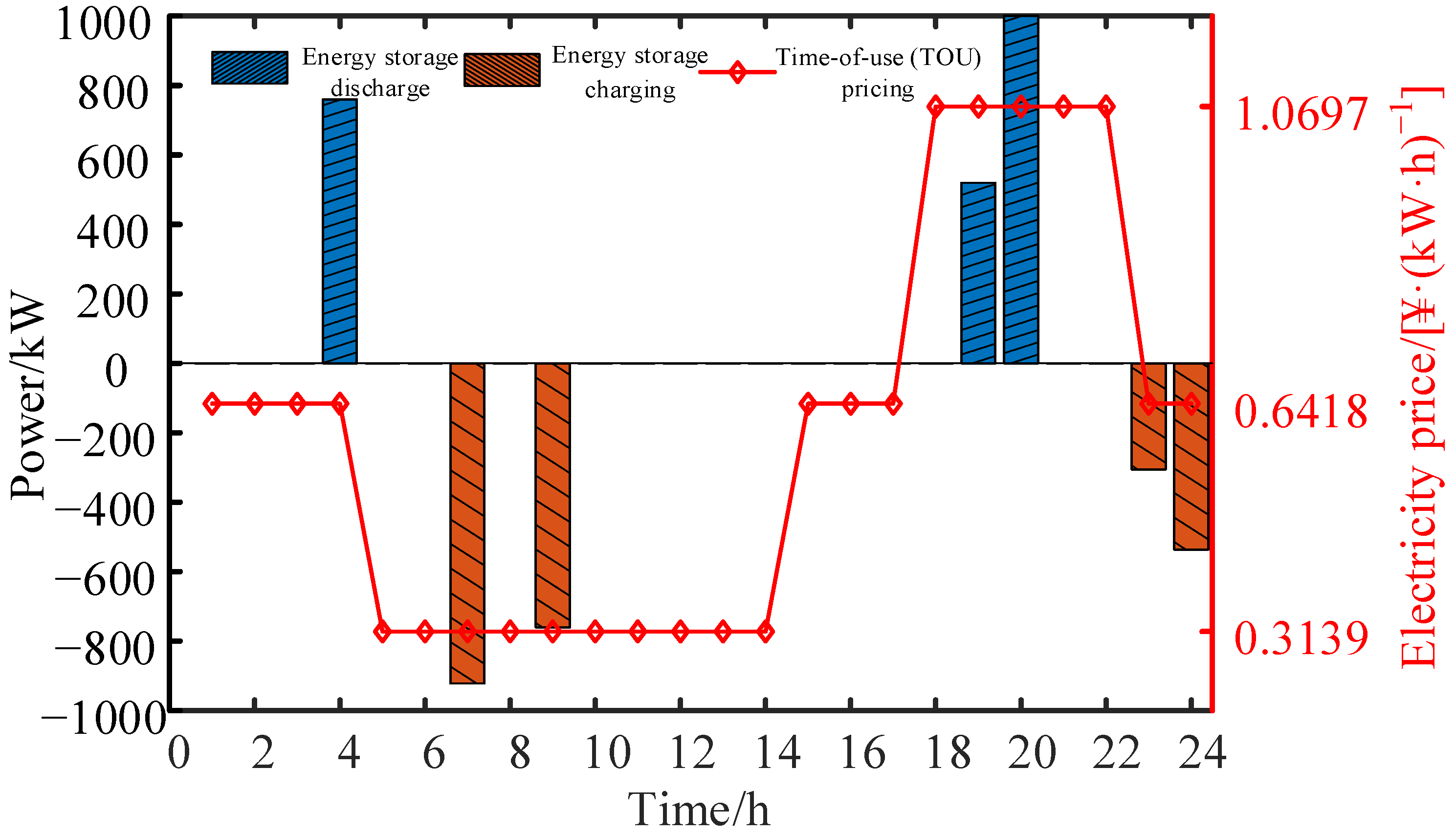
3.3.4. Constraints for Energy Storage and Distributed Photovoltaics
3.3.5. Overall Constraints of the Distribution Area
4. Solution Methodology for the Bi-Level Model
4.1. Model Preprocessing
4.2. Solving the Bi-Level Model Using ATC
| Algorithm 1: Analysis target cascading. |
| Step 1: Initialize parameters, . |
| Step 2: Given the expected values of tie-line power from the lower-level model, solve the upper-level model and record the resulting values of tie-line power , denoted as , respectively. |
| Step 3: Given the expected values of tie-line power from the upper-level model, solve the lower-level model and record the resulting values of tie-line power , denoted as , respectively. |
| Step 4: Determine convergence based on the convergence criterion given in Equation (45). If convergence is achieved, terminate the iteration. |
| Step 5: , update the Lagrange multipliers according to the update rule in Equation (46). Return to Step 2. |
5. Case Studies
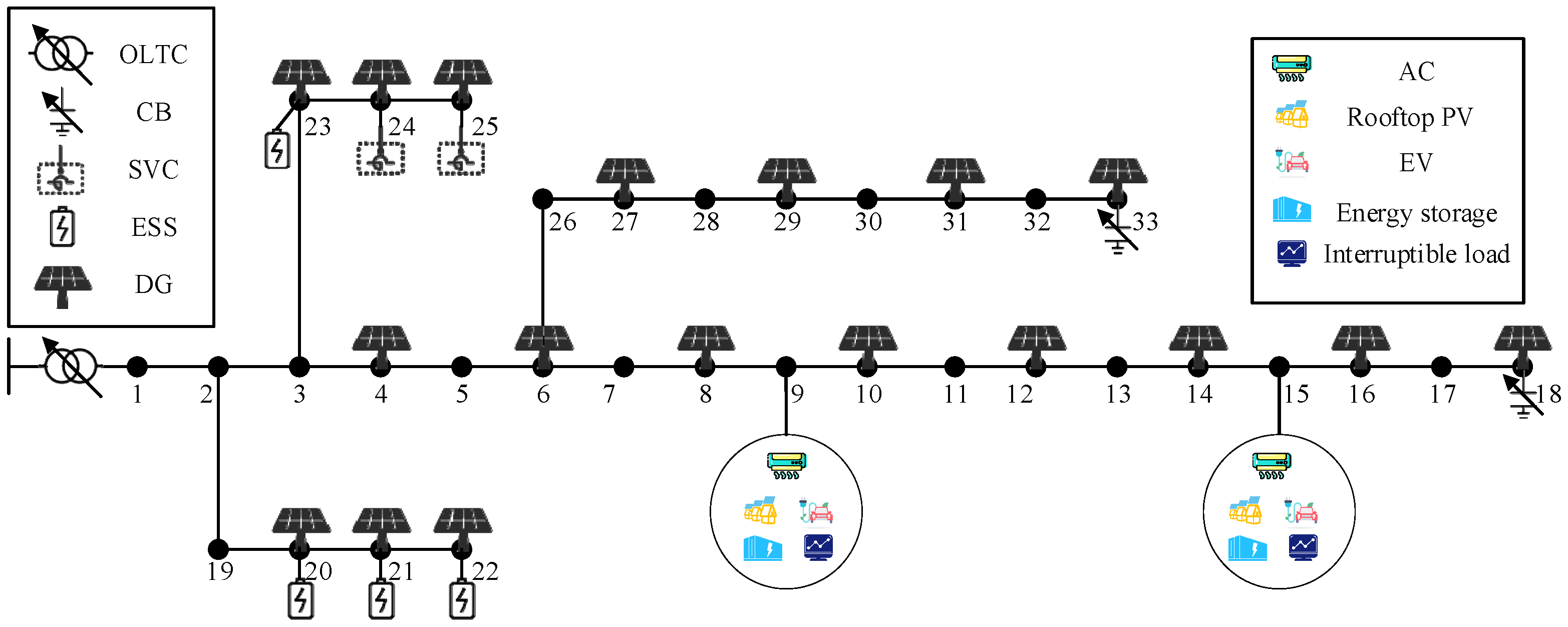
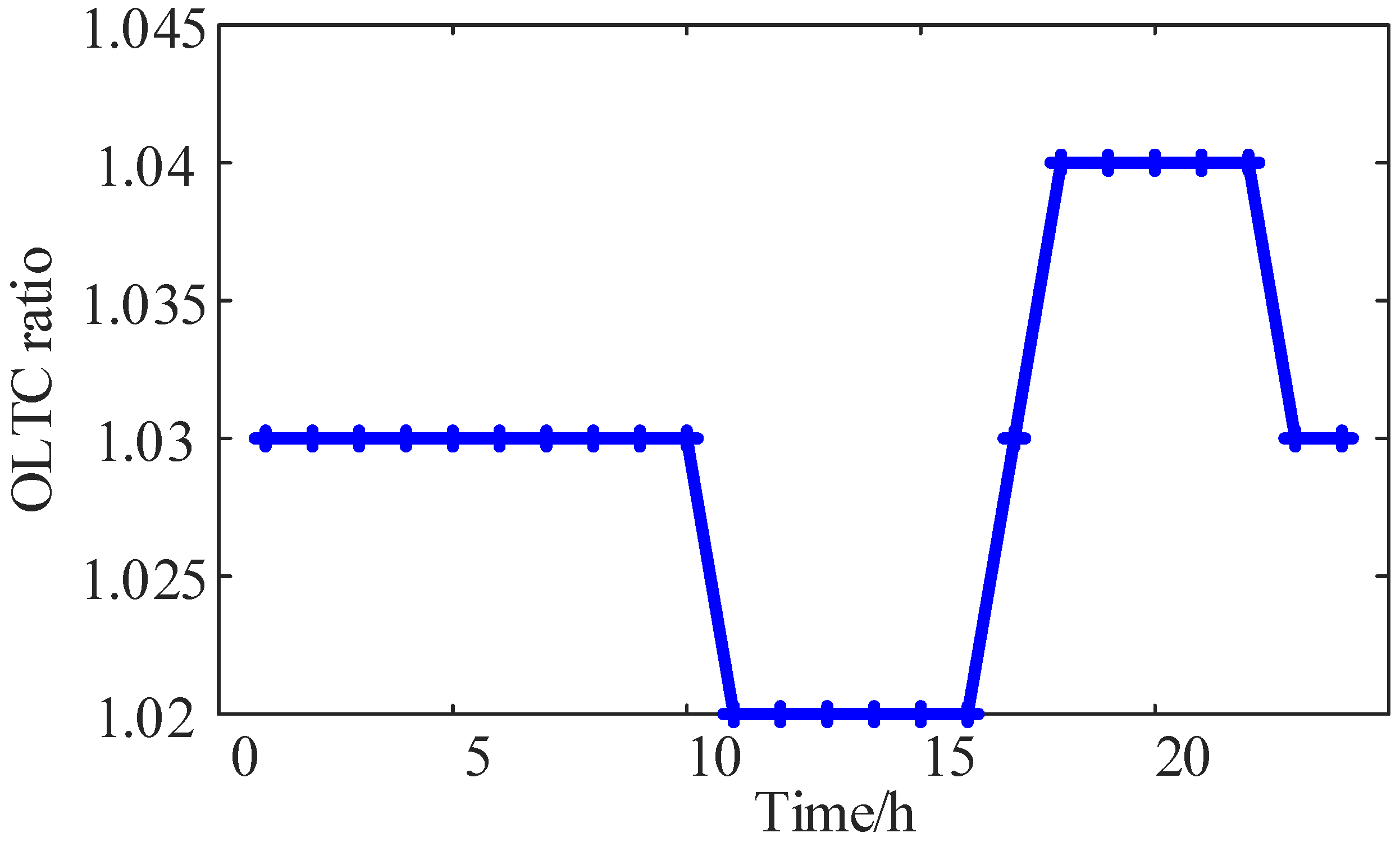
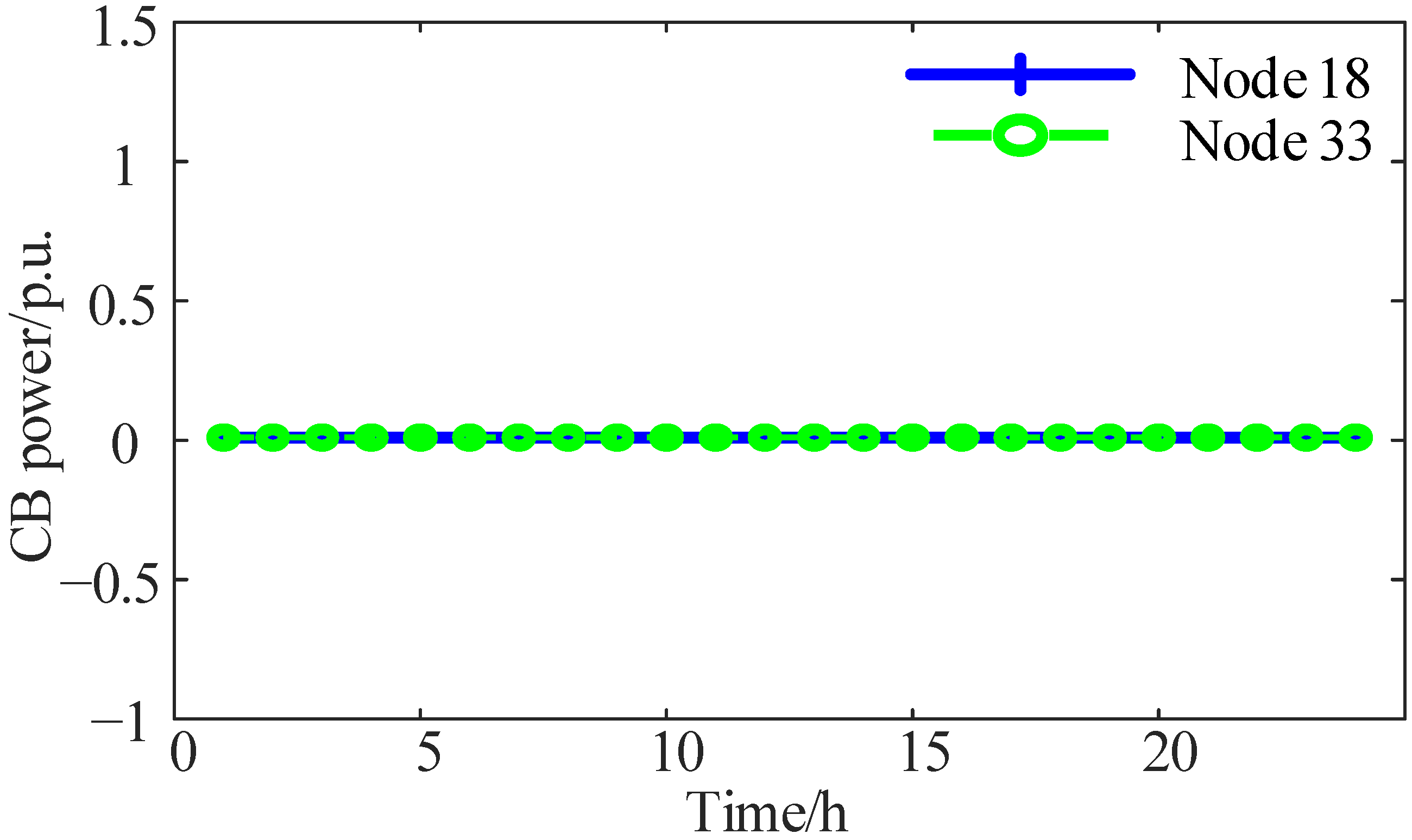
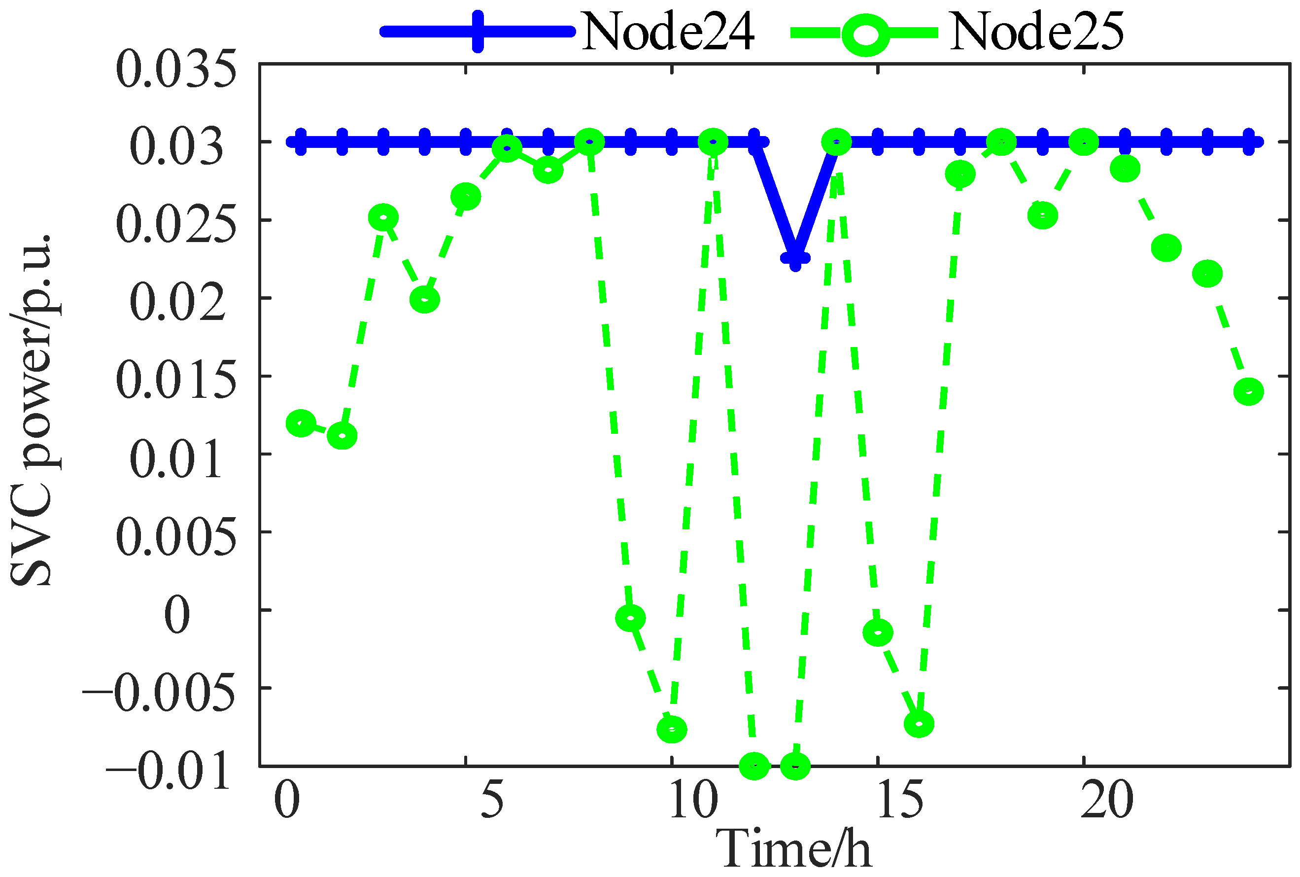
5.1. Analysis of Active Distribution Network Optimization Dispatch Results
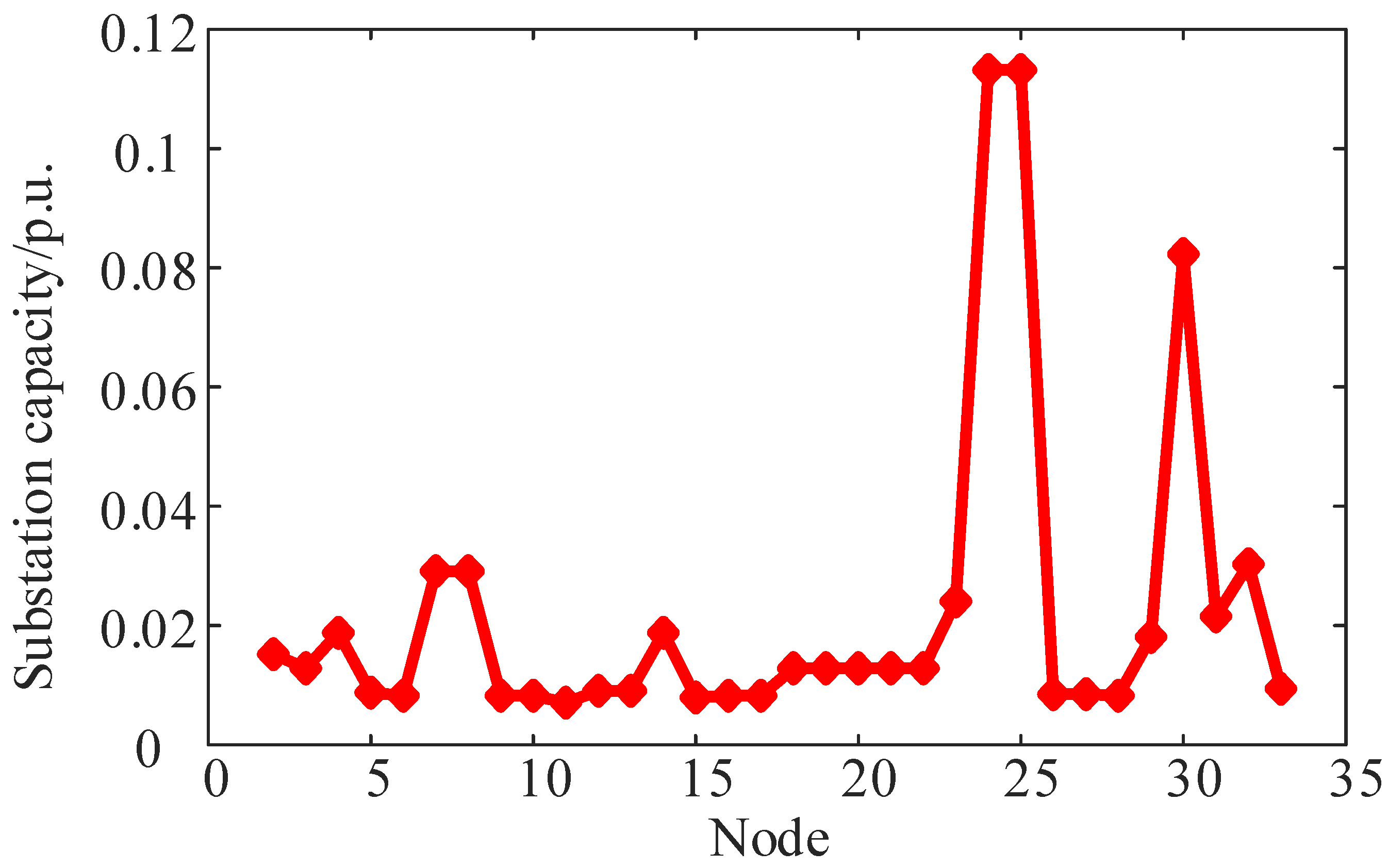
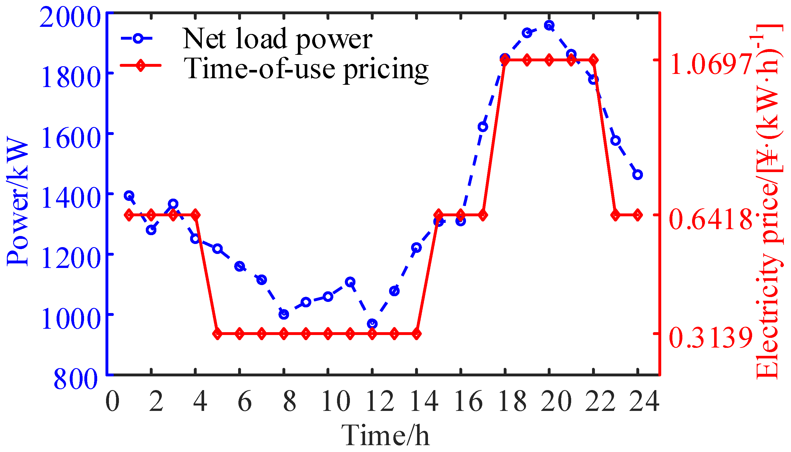
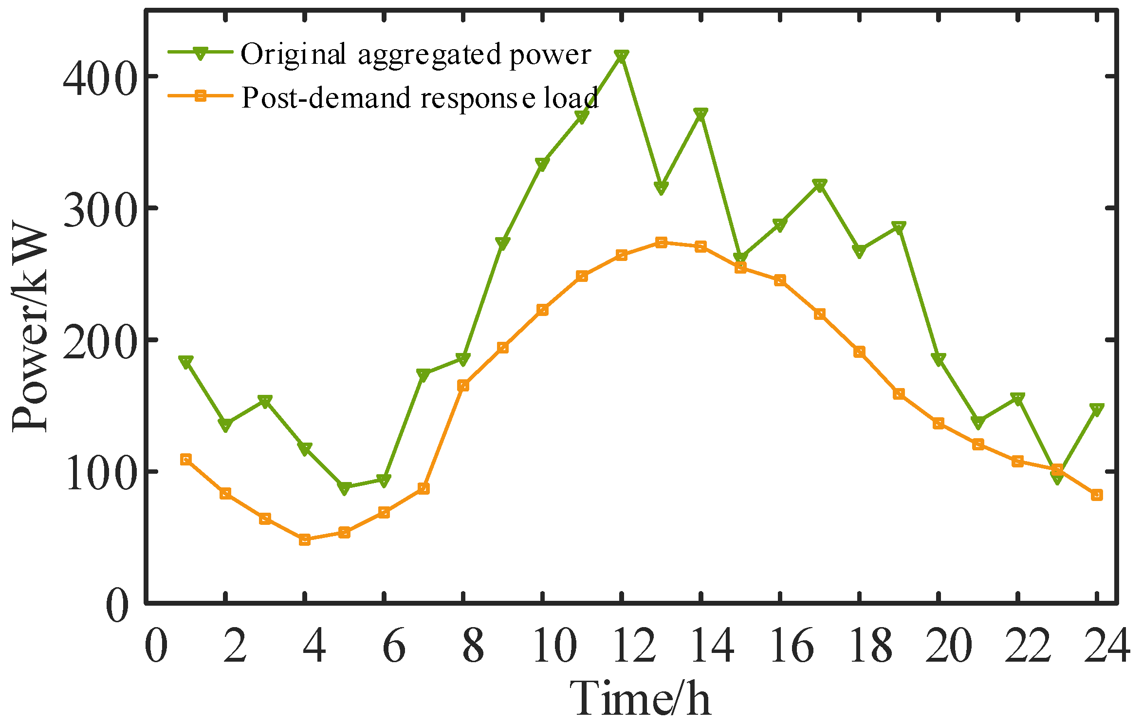
5.2. Analysis of Distribution Substation Optimization Dispatch Results
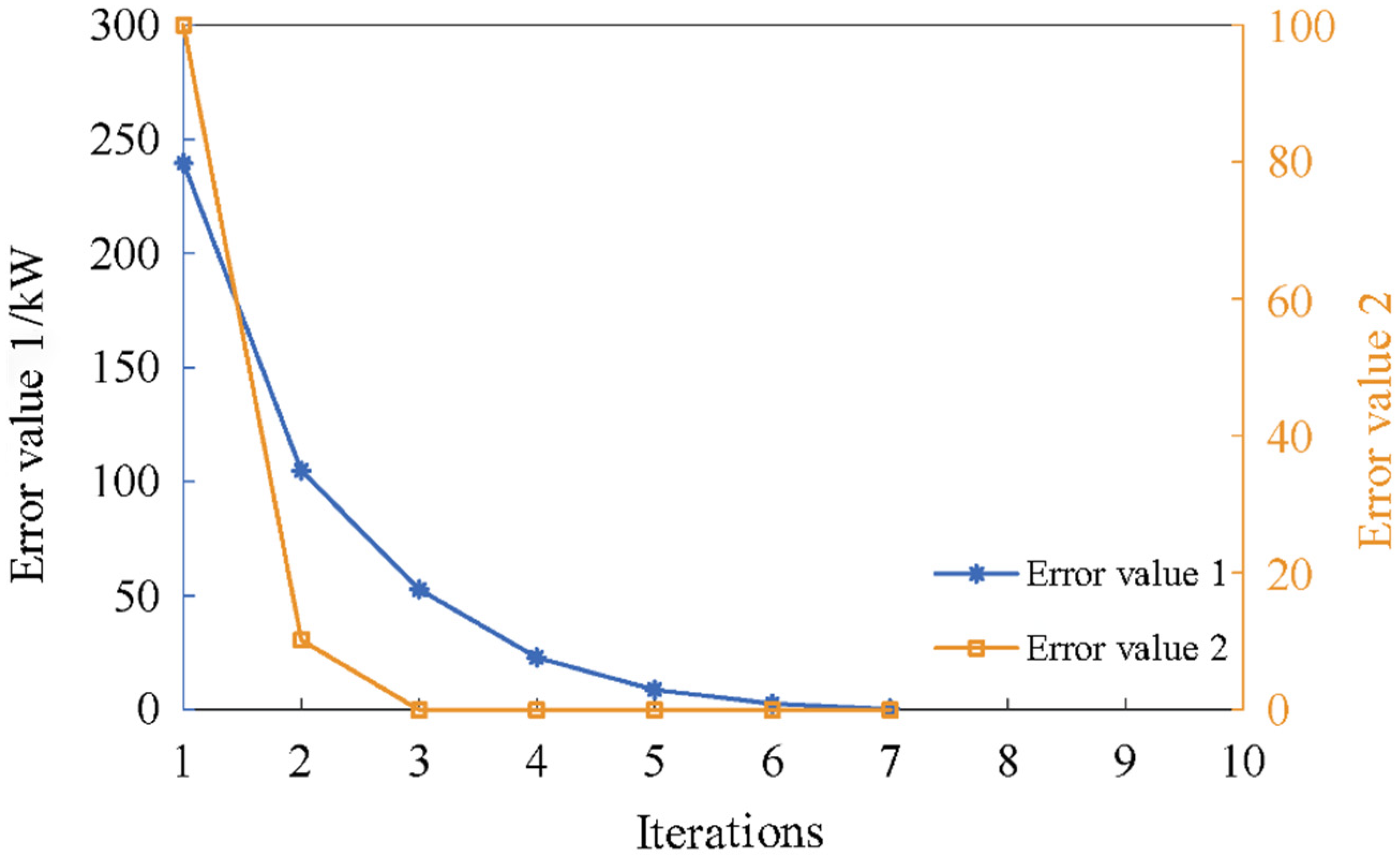
5.3. Analysis of Algorithm Solving Performance
6. Conclusions
Author Contributions
Funding
Data Availability Statement
Acknowledgments
Conflicts of Interest
Appendix A

| Name | Parameter Values | Name | Parameter Values |
|---|---|---|---|
| OLTC tap ratio range | 1 ± 6% | ESS charge and discharge power range/MW | 0~0.3 |
| Reactive power compensation capacity per single CB Bank/Mvar | 0.1 | ESS state of charge (SOC) range/MW h | 0.15~0.8 0.3 (initial) |
| SVC reactive power compensation range/Mvar | −0.1~0.3 | ESS charge and discharge efficiency | 0.9 (charge) 0.85 (discharge) |
| DG power limit ratio | 0.9 | DG power factor range | 0.95 (lead)~0.95 (lag) |
| Name | Parameter Values | Name | Parameter Values |
|---|---|---|---|
| 3.2 | 0.88 | ||
| 0 | 1 | ||
| /kW·h | 80 | /kW·h | 18.89 |
| 10.50, 19.00 | 2.14, 3.14 | ||
| /kW | 7 | 0.90 | |
| 30 | 1000 | ||
| [−0.040, 0.032, 0.024; 0.032, −0.032, 0.004; 0.024, 0.004, −0.024] | |||
| /% | 15 | /[¥·(kW·h)−1] | 0.3 |
| Name | Parameter Values | Name | Parameter Values |
|---|---|---|---|
| /[°C·(kW)−1] | [6, 16] | /[kW·h·(°C)−1] | [0.525, 0.57] |
| [2.6, 3.6] | /kW | 2 | |
| /°C | [21, 28] | /°C | 3 |
| /°C | 27.68 | /°C | 24.77 |
| /°C | 3 | 1000 | |
| /[¥·(kW·h)−1] | 0.3 |
| Name | Parameter Values | Name | Parameter Values |
|---|---|---|---|
| 3 | /% | 15, 10, 8 | |
| /% | 20, 20, 20 | /[¥·(kW·h)−1] | 0.5, 0.7, 0.8 |
| Name | Parameter Values | Name | Parameter Values |
|---|---|---|---|
| /kW | 1000 | /kW | 1000 |
| 0.95 | 0.95 | ||
| /kW·h | 1900 | /kW·h | 300 |
| 1000 | /[¥·(kW·h)−1] | 0.02 |
| Name | Parameter Values | Name | Parameter Values |
|---|---|---|---|
| 1000 | /[¥·(kW·h)−1] | 1.2 |
Appendix B

References
- National Development and Reform Commission; National Energy Administration. Guidance on High-Quality Development of Distribution Networks under New Circumstances. Available online: https://www.gov.cn/zhengce/zhengceku/202403/content_6935790.htm (accessed on 6 February 2024).
- Zhang, C.; Zhao, S.; Yang, H. Research on withstand performance test of internal short circuit fault of photovoltaic grid-connected inverter. High Volt. Appar. 2022, 58, 28–33. [Google Scholar]
- Huang, X.; Wu, H.; Li, M. Study on key factors affecting power supply performance of outdoor photovoltaic power. High Volt. Appar. 2021, 57, 36–42. [Google Scholar]
- Sansawat, T.T.; O’Donnell, J.; Ochoa, L.F.; Yao, X.; Zhu, Y. Decentralized voltage control for active distribution networks. In Proceedings of the 44th International Conference, Pittsburgh, PN, USA, 21–29 May 2022. [Google Scholar]
- Viawan, F.A.; Sannino, A.; Dalder, J. Voltage control with on-load tap changers in medium voltage feeders in the presence of distributed generation. Electr. Power Syst. Res. 2007, 77, 1314–1322. [Google Scholar] [CrossRef]
- Lu, J.; Ling, C. Analysis on lightning transient characteristics of PV module and array grounding system. Insul. Surge Arresters 2021, 4, 166–170. [Google Scholar]
- Xing, L.; Zhong, C.; Lijie, C.; Shengnan, R.; Xinyu, H. Local distributed voltage control in distribution networks with high permeability of PVs. Power Capacit. React. Power Compens. 2021, 42, 268–275. [Google Scholar]
- Rui, H.; Zhengang, X.; Yushu, C. Research on autonomous control method of photovoltaic inverter with active fault ride-through capability. High Volt. Appar. 2022, 58, 101–110. [Google Scholar]
- Angelim, J.H.; Affonso, C.M. Impact of distributed generation technology and location on power system voltage stability. IEEE Lat. Am. Trans. 2016, 14, 1758–1765. [Google Scholar] [CrossRef]
- Masoum, A.S.; Deilami, S.; Moses, P.S.; Masoum, M.A.; Abu-Siada, A. Smart load management of plug-in electric vehicles in distribution and residential networks with charging stations for peak shaving and loss minimization considering voltage regulation. IET Gener. Transm. Distrib. 2011, 5, 877–888. [Google Scholar] [CrossRef]
- Ye, L.; Qu, X.; Yao, Y. Analysis of intra-day time scale operation characteristics of wind-solar-hydro multi-energy complementary power generation system. Autom. Electr. Power Syst. 2018, 42, 158–164. [Google Scholar]
- Hu, D.; Ding, M.; Bi, R.; Liu, X.; Rong, X. Sizing and placement of distributed generation and energy storage for a large-scale distribution network employing cluster partitioning. J. Renew. Sustain. Energy 2018, 10, 25–31. [Google Scholar] [CrossRef]
- Chen, X.Y.; Wang, J.X.; Xie, J.; Xu, S.; Yu, K.; Gan, L. Demand response potential evaluation for residential air conditioning loads. IET Gener. Transm. Distrib. 2018, 12, 4260–4268. [Google Scholar] [CrossRef]
- Pourmousavi, S.A.; Patrick, S.N.; Nehrir, M.H. Real-time demand response through aggregate electric water heaters for load shifting and balancing wind generation. IEEE Trans. Smart Grid 2014, 5, 769–778. [Google Scholar] [CrossRef]
- Li, H.C.; Wang, X.W.; Yuan, Y.B.; Su, W.; Gong, Y. Simulation and analysis of electric water heater load regulation model based on direct load control. In Proceedings of the 2017 IEEE Conference on Energy Internet and Energy System Integration (EI2), Beijing, China, 26–28 November 2017; pp. 1–5. [Google Scholar]
- Zeng, L.K.; Sun, Y.; Ye, Q.Z.; Qi, B.; Li, B. A centralized demand response control strategy for domestic electric water heater group based on appliance cloud platform. IEEJ Trans. Electr. Electron. Eng. 2017, 12, S16–S22. [Google Scholar] [CrossRef]
- Zhou, N.C.; Xiong, X.C.; Wang, Q.G. Simulation of charging load probability for connection of different electric vehicles to distribution network. Electr. Power Autom. Equip. 2014, 34, 1–7. [Google Scholar]
- Zhang, L.; Yan, Z.; Feng, D.H.; Xu, S.; Li, N.; Jing, L. Two-stage optimization model based coordinated charging for EV charging station. Power Syst. Technol. 2014, 38, 967–973. [Google Scholar]
- Wang, C.H.; Tian, L.T.; Zhang, F.; Cheng, L. Optimal sizing of photovoltaic and battery energy storage of electric vehicle charging station based on two-part electricity pricing. In Proceedings of the 2020 IEEE Sustainable Power and Energy Conference (iSPEC), Chengdu, China, 23–25 November 2020; pp. 1379–1384. [Google Scholar]
- Sun, Y.P. Research on Dynamic Aggregation Model and Scheduling Mechanism of Demand Side Resources for Urban Power Grid. Ph.D. Thesis, North China Electric Power University, Beijing, China, 2018. [Google Scholar]
- Zhao, B.Y.; Xiong, C.; Zhang, P.C. Aggregation method of load virtual power plant based on cyber-physical system. Power Demand Side Manag. 2020, 22, 15–20, 27. [Google Scholar]
- Yibing, L.; Wenchuan, W.; Boming, Z.; Zhengshuo, L.; Zhigang, L. Multi-period Optimal Operation of Active and Reactive Power Coordination in Active Distribution Networks Based on Mixed-Integer Second-Order Cone Programming. Proc. CSEE 2014, 34, 2575–2583. [Google Scholar] [CrossRef]
- Feng, W.; Zhiqiang, L.; Keyong, Z.; Wang, G.; Yin, H.; Jia, Z.; Zhao, H.; Mi, Y. Aggregation and Scheduling of Controllable Resources in Distribution Areas Based on Time-of-Use Electricity Prices and Energy Storage Charging and Discharging Strategies. Energy Storage Sci. Technol. 2023, 12, 1204–1214. [Google Scholar] [CrossRef]
| Case Scenario | Comprehensive Objective/p.u. | Reverse Power Flow in Distribution Network/p.u. | Node Voltage Deviation/p.u. | Active Power Loss of Lines/p.u. | PV Active Power Curtailment/p.u. | PV Consumption Rate/% |
|---|---|---|---|---|---|---|
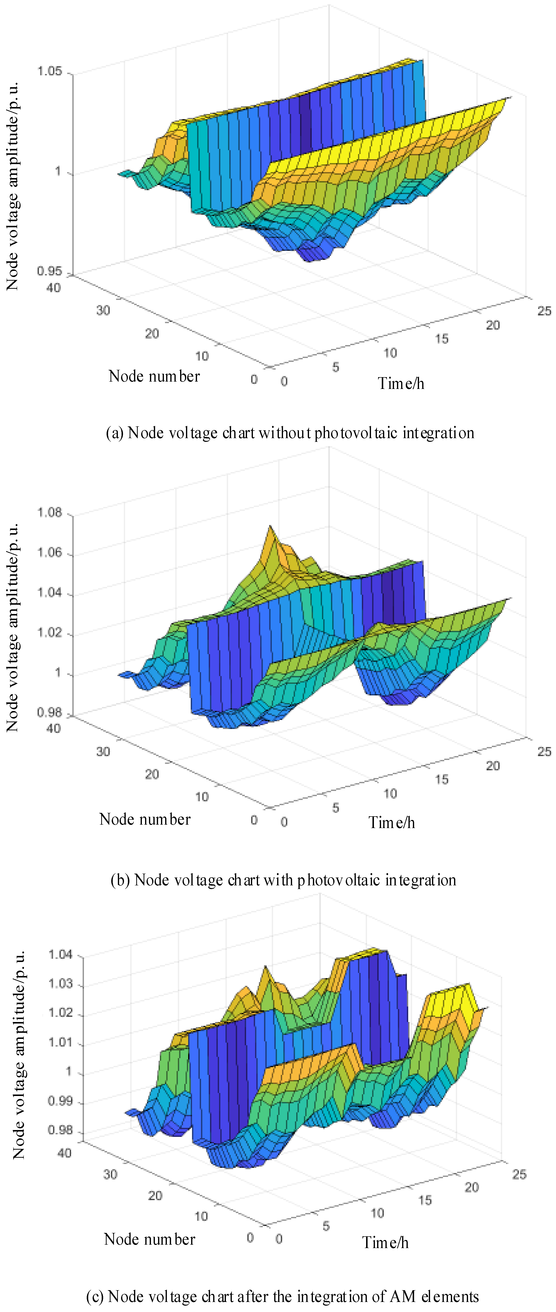
| Without photovoltaic integration | \ | 0 | 16.3738 | 0.2589 | \ | \ |
| With photovoltaic integration (penetration rate of 80%) | \ | 1.4561 | 19.2383 | 0.1676 | \ | \ |
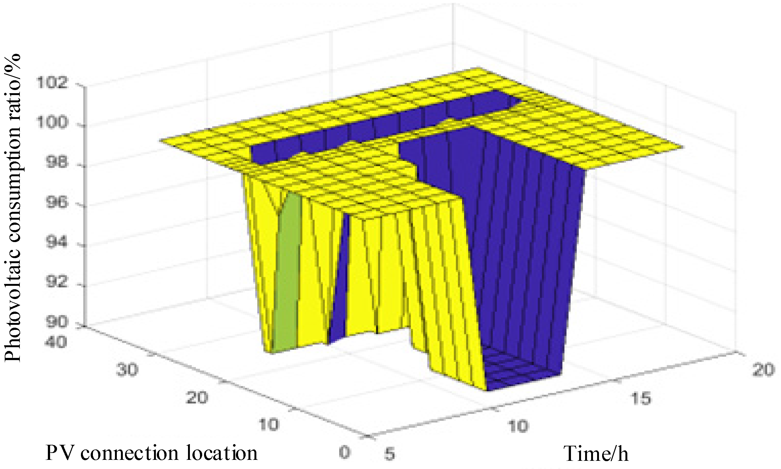
| AM | 0.1624 | 0.6783 | 11.1845 | 0.1429 | 0.1974 | 93.5597 |
| Name | /¥ | /¥ | /¥ | /¥ | /¥ | |
| Calculated value | 18,330 | 1391 | 0 | 96 | 19,817 | 0 |
Disclaimer/Publisher’s Note: The statements, opinions and data contained in all publications are solely those of the individual author(s) and contributor(s) and not of MDPI and/or the editor(s). MDPI and/or the editor(s) disclaim responsibility for any injury to people or property resulting from any ideas, methods, instructions or products referred to in the content. |
© 2024 by the authors. Licensee MDPI, Basel, Switzerland. This article is an open access article distributed under the terms and conditions of the Creative Commons Attribution (CC BY) license (https://creativecommons.org/licenses/by/4.0/).
Share and Cite
Zhao, Y.; Xue, Y.; Zhang, R.; Yin, J.; Yang, Y.; Chen, Y. Multi-Objective Optimization Operation of Multi-Agent Active Distribution Network Based on Analytical Target Cascading Method. Energies 2024, 17, 5022. https://doi.org/10.3390/en17205022
Zhao Y, Xue Y, Zhang R, Yin J, Yang Y, Chen Y. Multi-Objective Optimization Operation of Multi-Agent Active Distribution Network Based on Analytical Target Cascading Method. Energies. 2024; 17(20):5022. https://doi.org/10.3390/en17205022
Chicago/Turabian StyleZhao, Yiran, Yong Xue, Ruixin Zhang, Jiahao Yin, Yang Yang, and Yanbo Chen. 2024. "Multi-Objective Optimization Operation of Multi-Agent Active Distribution Network Based on Analytical Target Cascading Method" Energies 17, no. 20: 5022. https://doi.org/10.3390/en17205022
APA StyleZhao, Y., Xue, Y., Zhang, R., Yin, J., Yang, Y., & Chen, Y. (2024). Multi-Objective Optimization Operation of Multi-Agent Active Distribution Network Based on Analytical Target Cascading Method. Energies, 17(20), 5022. https://doi.org/10.3390/en17205022