Machine Learning-Based Automated Fault Detection and Diagnostics in Building Systems

Abstract

Automated fault detection and diagnostics analysis in commercial building systems using machine learning (ML) can improve the building’s efficiency and conserve energy costs from inefficient equipment operation. However, ML can be challenging to implement in existing systems due to a lack of common data standards and because of a lack of building operators trained in ML techniques. Additionally, results from ML procedures can be complicated for untrained users to interpret. Boolean rule-based analysis is standard in current automated fault detection and diagnostics (AFDD) solutions but limits analysis to the rules defined and calibrated by energy engineers. Boolean rule-based analysis and ML can be combined to create an effective fault detection and diagnostics (FDD) tool. Three examples of ML’s advantages over rule-based analysis are explored by analyzing functional building equipment. ML can detect long-term faults in the system caused by a lack of system maintenance. It can also detect faults in system components with incomplete sets of sensors by modeling expected system operations and by making comparisons to actual system operations. An example of ML detecting a failure in a building is shown along with a demonstration of the soft decision boundaries of ML-based FDD compared to Boolean rule-based FDD analysis. The results from the three examples are used to demonstrate the strengths and weaknesses of using ML for AFDD analysis.

1. Introduction

Machine learning (ML) has seen an increase in popularity for automated fault detection and diagnostics (AFDD) in building systems in recent years [1,2]. Previous work [3] describes a method for processing data into standardized formats and outlines the use of classification algorithms to detect and diagnose faults in building systems. This paper serves as a continuation of research conducted in the previous work by implementing the described methods in a building on the Texas A&M Campus in College Station, Texas. The implementation of research methods in a real system, along with discussion of the resolutions to problems encountered during implementation, advances research from experimental to practical analysis. In addition to classification algorithms, anomaly detection algorithms were evaluated for use in AFDD in building systems.

Short-term system failures are those which occur suddenly, such as a fan going offline. Detecting short-term failures in system components is discussed in the low temperature alarm section. Long-term system failures are those which progress in severity over time, such as progressive clogging of strainers in chilled water piping systems. Detecting long-term system failures is discussed in the clogged chilled water pump strainer section. The clogged chilled water pump strainer section also discusses preemptively detecting long-term system faults before they have a negative impact on building conditions.

Physical building system operation is governed by first-principle equations with loss terms due to system inefficiencies. When using data measured from a real building, ML can create a model of the building’s performance with loss terms. ML algorithms are trained using a dataset of building measurements taken during a baseline period consisting of internal and external building conditions. The trained model learns the relationship between the building conditions and the model’s output, which is a categorical value representing fault-free or faulty states. In the evaluation period, the building will acquire new data which can be evaluated by the trained model. The trained model will use the new set of data as inputs and calculate an output based on the relationships it learned from the baseline dataset. When measured behavior deviates from the expectations learned from the baseline period, notifications will be sent to building operators of the change in behavior. This usage of ML is discussed in the enthalpy recovery wheel slipping section.

The ML methods described above are applied to data measured from the 525 kft² (49 km²) Zachry Engineering Complex building on the Texas A&M University campus in College Station, Texas.

Comparisons between Boolean Rule-Based FDD and ML-Based FDD

Boolean rules are the current standard in AFDD procedures in commercial buildings [4]. Boolean rules can be effective in detecting known faults by defining thresholds of normal operation and flagging measurements beyond those thresholds as faulty, although diagnostics using Boolean rules is usually a manual process requiring expert knowledge. For example, a Boolean rule can be defined to detect high space temperatures by defining a threshold of 78 °F. Any space temperature measurements above 78 °F will be collected and sent to a building operator for diagnostics. Boolean rules can be restrictive in applications because they must be defined individually and strictly detect behavior beyond their defined thresholds. Any progressive failures will remain undetected until their severity surpasses the threshold definition.

Machine learning, however, can learn unique building behaviors by using a single configuration. When configurations are defined in a general way, as described in Section 3 of this paper, the algorithm can be applied to different buildings using a single definition. ML algorithms can also detect progressive failures more successfully than Boolean rule-based approaches, described in Section 4 of this paper. ML algorithms are also able to learn the energy transfer governing equipment operation in the building automatically, as described in Section 5 of this paper. Finally, ML algorithms are able to detect undefined faults in the system, as described in Section 6 of this paper.

2. Classification and Anomaly Detection Algorithms

Both classification and anomaly detection algorithms are used in this project to analyze the Zachry building. Classification algorithms categorize data using a set of input variables. The categorizations made by classification algorithms represent fault states in the system. Anomaly detection algorithms identify outliers in datasets by using binary classification: their outputs represent either baseline or outlier states.

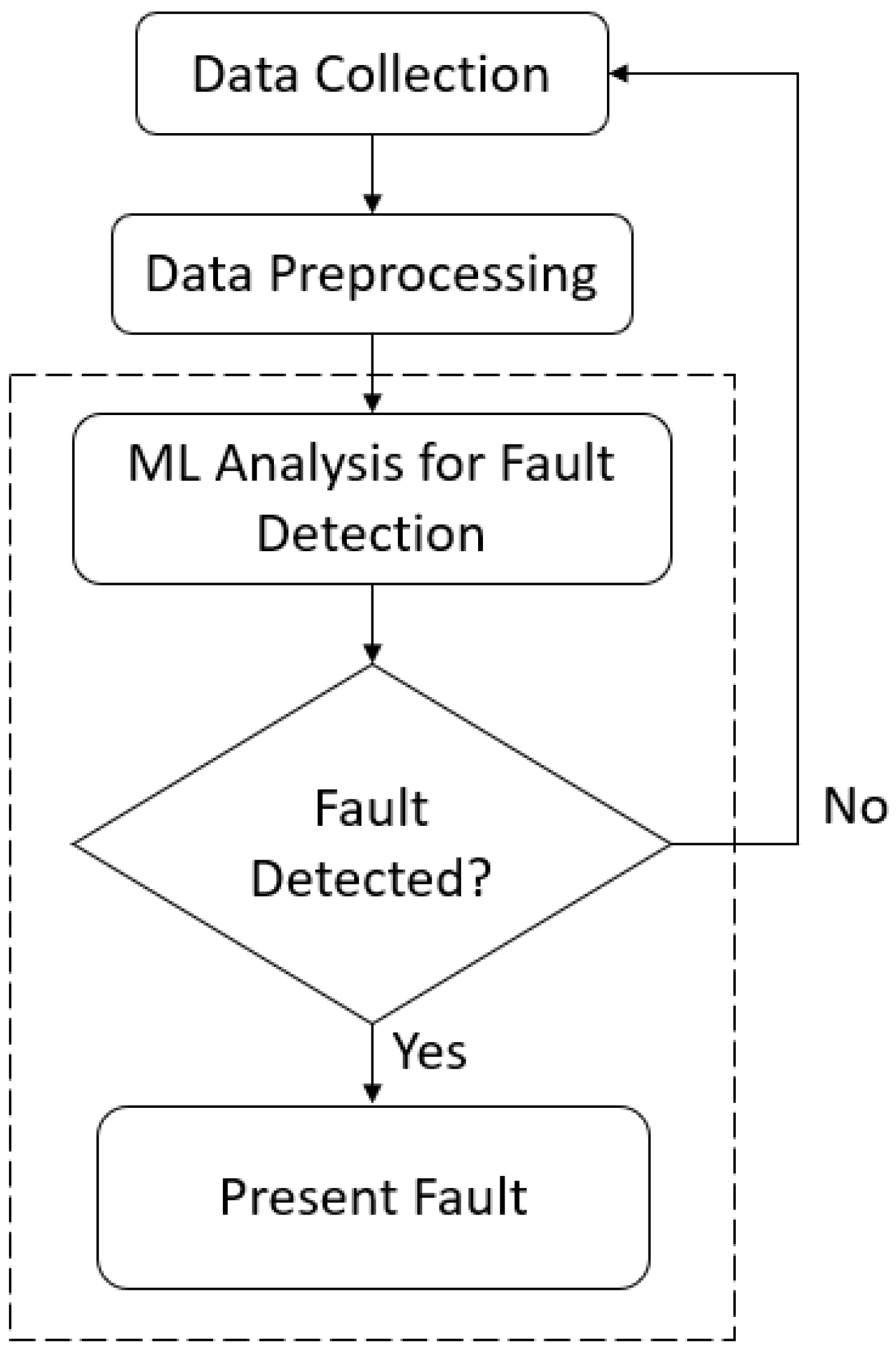
The flowchart shown in Figure 1 shows the procedure for applying ML to building data for FDD. Data collection is performed by the BMS, where measured data are exported into a local database for further processing. Data preprocessing is described in Section 3 of this paper. The design of ML Analysis for Fault Detection is described in previous work [3], though its applied use is described in Section 4, Section 5 and Section 6 of this paper.

2.1. Classification

Classification analysis in this project is performed using the LightGBM framework in ML.NET v1.7.0, which uses gradient-boosted decision trees for analysis and has been described by Ke et al. in a reference paper [5]. LightGBM is an open-source project which can be found in Microsoft’s online repositories [6].

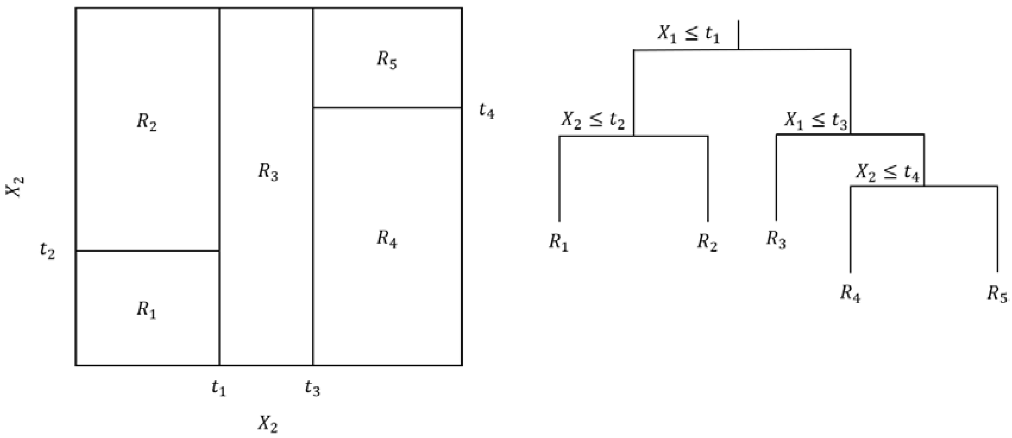
LightGBM was chosen as the algorithm for this research due to its use of decision trees. Hastie et al. state that decision trees “partition the feature space into a set of rectangles, and then fit a simple model…in each one” [7]. A graphical representation of a decision tree model is shown in Figure 2. In Figure 2, the $R_i$ parameters represent regions in the feature space attributed to a specific output class. The $X_i$ parameters represent the features of the dataset. In the example, only two features are used for simplicity in the visualization. The $t_i$ parameters represent the values at the decision nodes of the tree, where the defined feature value is compared to the decision node value to determine which branch of the tree to follow.

Decision trees have also been used successfully in existing research. Yan et al. developed decision trees to detect various faults in an air handling unit (AHU), including leaking coil valves, stuck coil valves, or stuck dampers [8]. The authors demonstrate the interpretability of decision trees by analyzing their trained model and describing its branching conditions, similar to those shown in the left image of Figure 2. For example, the authors explain the decision tree classifies behavior as a cooling coil valve stuck at fully closed when the supply air temperature is greater than 19.2 °C (66.6 °F). Though a supply air temperature of 19.2 °C may be caused by other faults in the system, like a stuck open outside air damper, the authors clarify that the “analysis is based on the faults investigated in this study without considering other possible AHU faults.” The cooling coil valve stuck at fully closed is the only fault investigated in their study that could result in a supply air temperature greater than 19.2 °C.

Decision trees were used in this study due to the interpretability of their processes. The evolution of AFDD from Boolean rules to decision trees is natural because both algorithms define thresholds for building behavior and generate results based on the comparison between system measurements and the algorithm’s thresholds. In the previous paragraph, the authors explained that the cooling coil valve is stuck at fully closed when the supply air temperature is greater than 66.6 °F. This fault could also be detected using Boolean rules in a similar way: defining a rule that detects when the supply air temperature measurements in the building are greater than 66.6 °F. By using decision trees for ML analysis, building operators familiar with Boolean rules already understand the logic of the ML algorithm, which can build trust in its results.

2.2. Anomaly Detection

Anomaly detection algorithms serve to detect “patterns in data that do not conform to expected behavior” [9]. Anomaly detection analysis provides fault detection by distinguishing between the baseline (expected) and abnormal system states. The abnormal system states represent unexpected system operation caused by a fault.

Anomaly detection analysis in this research is performed using principal component analysis (PCA) with a randomized singular value decomposition, called randomized PCA. Randomized PCA uses randomized algorithms to partially decompose the dataset into the subspace that captures the “most action” of the dataset. The decomposed dataset is then reduced further by PCA. Halko et al. described the randomized PCA algorithm in their publication [10].

Anomaly detection is used in this research to detect faults in the Zachry system, which lack a simulation definition. Anomaly detection datasets are defined to generally monitor equipment and include the equipment inputs, outputs, and command values. Anomaly detection algorithms are used to detect any deviations from expected baseline behaviors. These deviations can be attributed to a change in system operation, which may be caused by a fault.

While anomaly detection algorithms are simpler to configure, the reliance on manual diagnostics procedures can limit the appeal to operators wishing to automate the fault detection and diagnostics procedures. An example of the procedure of fault detection using anomaly detection is shown in this paper, as well as the relative complexity of fault diagnostics once the detection has been made.

3. Data Preprocessing

The goal of data preprocessing in ML analysis is to improve the quality of data used to train an ML algorithm. Data preprocessing may involve output class balancing in the training dataset, input variable (feature) selection, or the correction of erroneous measurements from the training dataset.

3.1. Output Class Balancing

Output class balancing can resolve the imbalanced representation of output classes in the training dataset. An imbalanced representation of each output class in the training dataset can reduce the quality of the model. Ebrahimifakhar et al. conducted a classification analysis using an imbalanced dataset, where only 1.5% of the training dataset was labeled as fault-free data [11]. The authors found that only one of the nine tested classifiers, quadratic discriminant analysis, was able to classify the fault-free state correctly. The authors suggested that the cause of the low success rate of detecting fault-free states could be the balance of their training dataset, which contained 98.5% faulty data. Bode et al. also conducted a study with an imbalanced dataset and concluded that an imbalanced dataset can bias results [12]. The authors stated that the models trained using imbalanced datasets “were unable to identify the faults as they were noted by the operation staff.”

The simulation procedures used in this work were designed to guarantee a balanced output class representation in the training datasets for the classification analysis used in Section 4 and Section 5. For each data point measured from the system, a second data point will be generated representing faulty system operation. The simulation procedures are described in previous work [3]. Those procedures expand on the procedures developed by Shohet et al. in their work [13], where faults were simulated into a dataset with severities at 5% intervals between 1% and 45%. Shohet’s decision tree model was able to classify over 95% of faults in the testing dataset.

3.2. Feature Selection

Chandrashekar et al. studied the effects of feature selection on ML models [14]. The authors analyzed datasets found in the UCI machine learning repository [15]. The authors found that in the repository’s Ionosphere dataset, reducing the number of features from 34 to 9 improved the model’s prediction accuracy from 90% to 95%. The reduced feature set was selected using the sequential floating forward selection (SFFS) algorithm and the reduced dataset was analyzed using a support vector machine. However, in using the repository’s diabetes dataset, reducing the number of features from 8 to 7 reduced the model’s prediction accuracy from 80% to 71%. This prediction accuracy was also calculated using the SFFS algorithm with a support vector machine. The authors’ conclusions are that the number of features should be determined by cross-validation, where different sets of features are defined and only the model with the highest prediction accuracy is used for analysis. When removing features, the objective is to remove selected interdependent features in the order of high to low dependence until the prediction accuracy peaks. The research discussed in this paper implements a cross-validation procedure for feature selection, where subsets of the original feature set are analyzed using the user-defined algorithm. The highest-performing feature set is saved for future analysis of the data.

3.3. Standardized Data Formats

Data from the Zachry system were preprocessed into a standardized format like the propositions by Project Haystack [16] and Brick Schema [17]. Both initiatives propose standardized data models that label building data semantically, in human-readable phrases such as the AHU 1 cooling coil valve command instead of AHU-01-CC-CMD.

Standardizing data labels allows for similar trends, such as cooling coil commands from different AHUs, to be analyzed in similar ways. Their individual performance can be analyzed en masse by referring to the standardized label instead of a specific trend. Semantic labels also simplify analysis for building operators, who may work with buildings on different building management systems that use unique point naming conventions.

In addition to semantic labeling, the preprocessing procedure implements point organization which describes the point’s physical location in the system by a defined hierarchy of equipment. Figure 3 shows a sample AHU with n variable air volume (VAV) boxes which each measure m points. In the diagram, each VAV box measures the same points but in real buildings, the actual sensor/actuator points measured by different VAV boxes may vary. The different measurements could be caused by varying box configurations throughout the building. For example, in the Zachry building, there are two configurations of terminal boxes. One configuration uses reheat coils to condition the supply air served to the box while the other directly outputs supply air from the AHU. Both configurations use dampers to control flow to the space. The AHU also measures x points, such as the cooling coil command or mixed air temperature. Knowing the equipment hierarchy in the system enables the analysis of parent and child relationships, such as the effect of a faulty cooling coil in the AHU on the space temperatures of each zone it serves.

The combination of standardized data labels and the defined point organization scheme allow ML models to be defined in a generic way and applied across several different campuses. Dataset features and fault simulations used in this work are defined by standardized labels, as mentioned in previous work [3]. These standard labels are used to categorize trend data across several different projects. Because the datasets and the project data are defined in the same standardized way, the datasets may be referenced in each of those projects. In this way, datasets may be collected from different projects using a single definition. ML models can be trained and tested using each of the datasets collected using the standardized scheme.

3.4. Hierarchical Organization

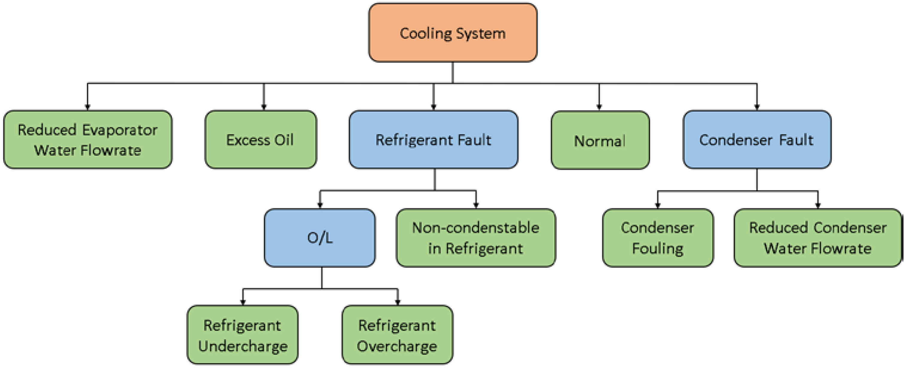
Li et al. used decision trees to detect faults in building cooling systems [18]. The authors processed their data into a tree-structured fault dependence kernel, which organizes seven faults into a hierarchy of ancestors and descendants. Figure 4 shows the fault hierarchy tree as designed by the authors. The tree shows that when measured data are classified as a refrigerant fault or condenser fault, additional analysis is performed to classify the descendent fault. The authors found that the tree-structured fault dependence kernel achieved a classification accuracy greater than 90%.

The tree developed by Li et al., shown in Figure 4, represents technical behavior in the system by categorizing faults. In Figure 4, the categorized faults belong to the cooling system. The tree developed in Figure 3 represents the equipment hierarchy of an air-side system. Similar trees have been developed for cooling and heating systems.

This work expands on the tree-structured analysis developed by Li et al. by analyzing faults based on their defined equipment categories. For example, a cooling coil fault occurs in the air handler and chilled water faults occur in the cooling system. As part of the analysis, users are required to select equipment for analysis. Organizing faults by equipment type allows for the full set of faults to be automatically filtered to those relevant to the selected equipment. If a user defines the analyzed equipment to be a cooling system, only faults with the cooling system type will be analyzed.

4. Clogged Chilled Water Pump Strainer

The Zachry building receives cooling and heating water from the campus’s district system. Zachry’s chilled water system measurements include water inlet/outlet pressures, water flows, water temperatures, and on/off statuses of the pump. The water flow is controlled by a variable speed controller for the pump. When the differential pressure rises above the setpoint, the pump motor speed is lowered. When the differential pressure drops below the setpoint, the pump motor speed is raised.

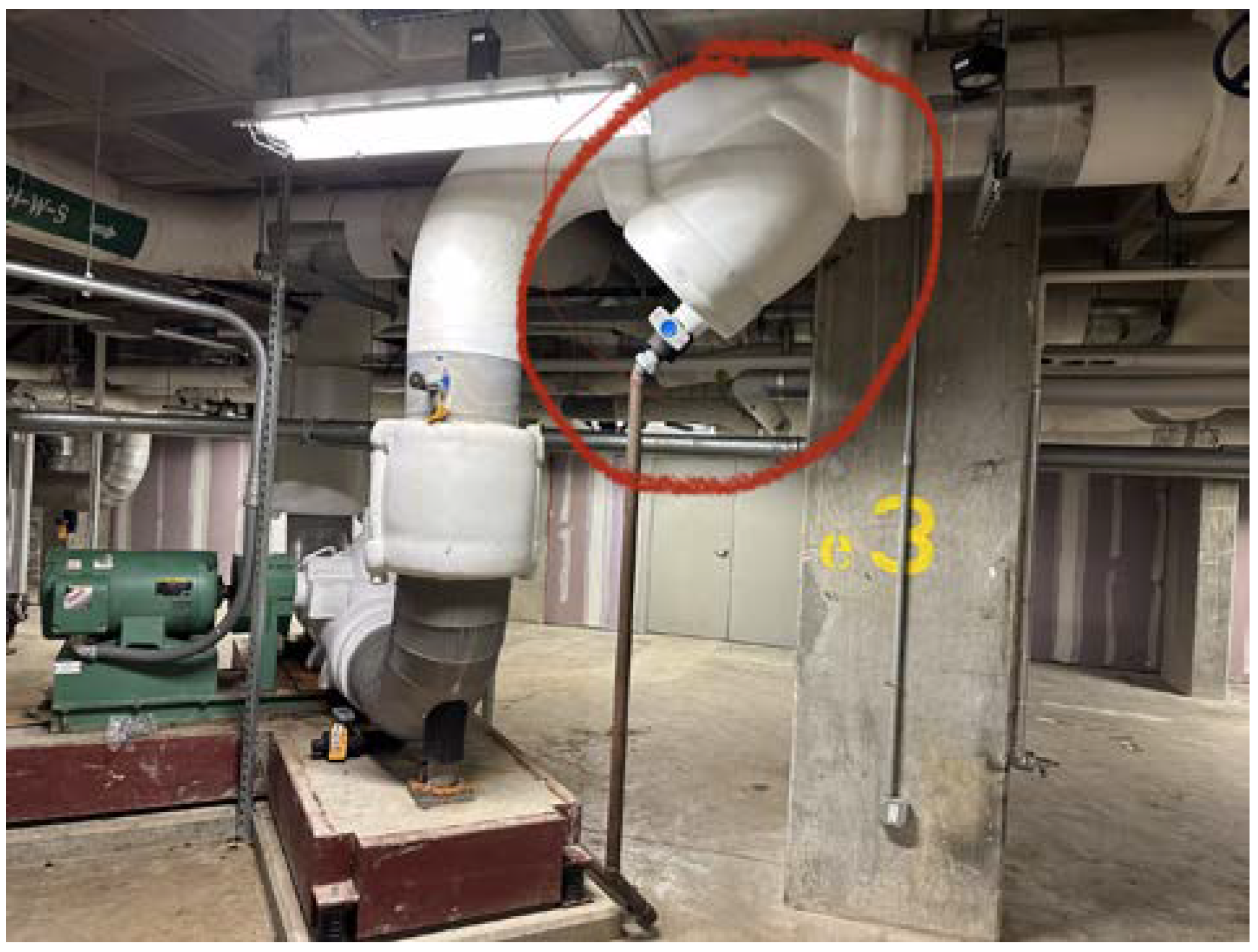
Between the campus supply pressure sensor and the pump is a strainer, circled in red in Figure 5. This strainer is responsible for blocking objects like small rocks or other debris from entering the pump, which could cause damage if allowed to enter the pump’s impeller. The debris may enter the chilled water system from leaks in pipes due to surface corrosion or improper cleaning after new pipes are installed or pipe breaks are repaired. The strainers should periodically be cleaned of all debris to allow for unobstructed flow between the campus supply pipe and Zachry’s chilled water pumps. The strainers are cleaned by briefly redirecting chilled water flow into a drainage system and allowing the debris to flow out of the building’s chilled water pipe. Once the debris has been drained, water flow is directed back into Zachry’s chilled water pumps.

When debris collects in the strainers, chilled water flow is partially obstructed from entering Zachry’s pumps. If flow is obstructed in the pipe, the controls will command the pumps to run at a higher speed. In severe cases, the pumps will be unable to overcome the blockages in the strainers even when running at 100% speed. If the strainer is allowed to continue collecting debris without being cleaned, the building’s supplied chilled water flow rate and its supplied pressure will begin to drop, which can result in higher supply air temperatures. The higher supply air temperature may result in higher space temperatures in all zones served by the AHU.

4.1. Case Study in Zachry

An ML model designed to detect clogged strainers in the chilled water system must define a set of relevant system measurements used as model inputs (features). The relevant system measurements to detect a clogged strainer in Zachry’s chilled water system are the following:

• Campus supply pressure;
• Pump speed command;
• Primary chilled water flow rate;
• Building supply pressure.

4.1.1. Campus Supply Pressure

The campus supply pressure measurement is used to validate the model inputs listed above. Zachry pumps are sized so that when other campus pumps are operating properly and producing expected supply pressures, the Zachry pumps are able to increase the pressure of chilled water supply to the building and meet the ΔP setpoint. However, if campus pumps malfunction or if neighboring buildings require an abnormal amount of chilled water, the chilled water supply pressure from the campus will drop and the Zachry pump may be unable to produce enough pressure to meet the ΔP setpoint.

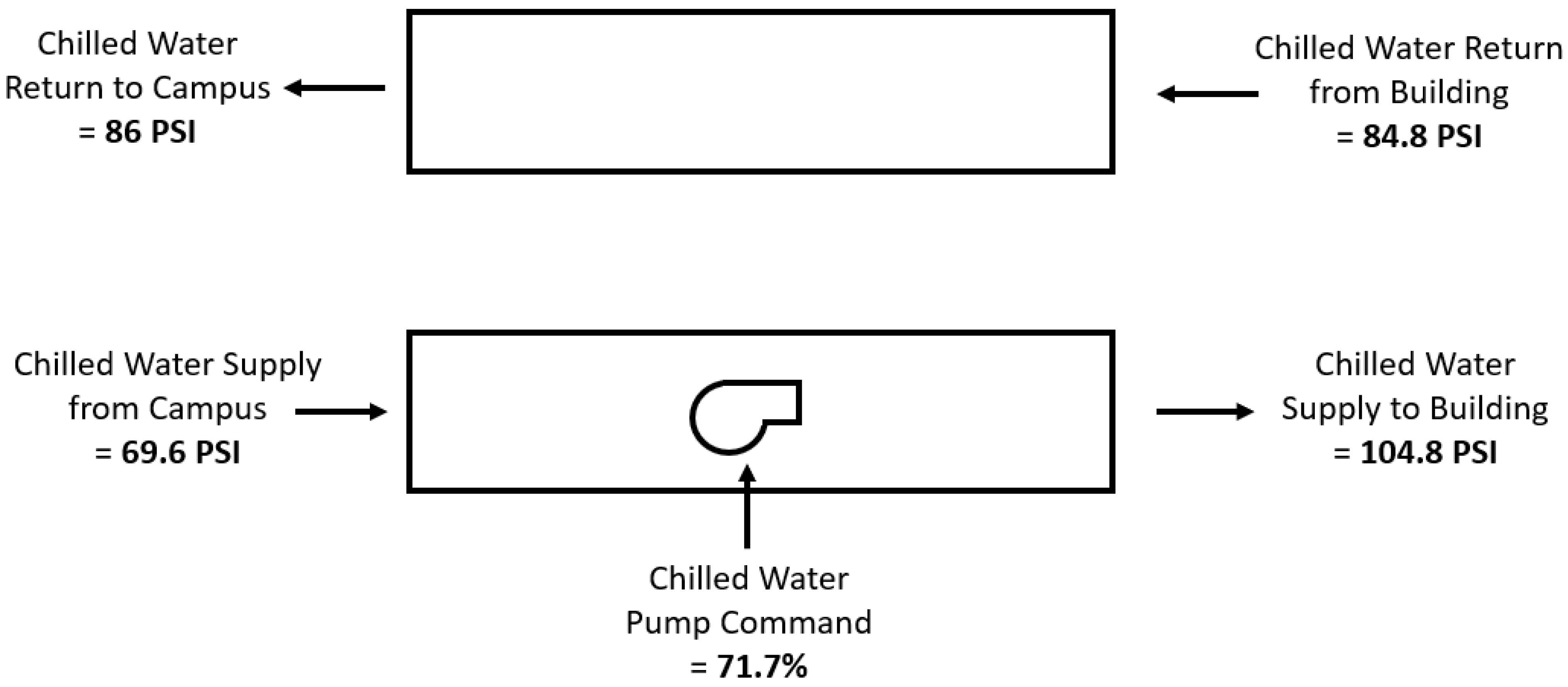
Consider the measurements shown in Figure 6, which were taken during normal system operation on 28 September 2023, at 2:30 P.M. The chilled water supply pressure (ChWS) from the campus is 69.6 PSI and the chilled water return pressure (ChWR) to the campus is 86 PSI. This is a campus ΔP of 16.4 PSI. The ChWS to the building is 104.8 PSI, which means the pump produced a pressure rise of 35.2 PSI at a speed command of 71.7%. The ChWR from the building is 84.8 PSI, which means the building ΔP is 20 PSI and is meeting the setpoint.

If the ChWS from the campus falls to 50 PSI due to issues such as those described at the beginning of this subsection, Zachry’s chilled water pump will run at 100% to maintain the building ΔP setpoint of 20 PSI. Using the ChWR from the building shown in Figure 6, the ChWS must be 104.8 PSI. If the ChWS from the campus falls to 50 PSI, the pump will be unable to produce the 54.8 PSI pressure rise required to meet the building ΔP setpoint.

As described previously, a clogged strainer in the system can be detected by data analytics when the chilled water pumps are run at 100% and the building supply pressure value drops (and therefore the ΔP setpoint is not met). This behavior is identical to the expectation when the campus ΔP is high, as described in the previous paragraph. To distinguish between the two causes of unmet building ΔP setpoints, the campus supply pressure measurement should be used. If the ChWS from the campus is low, the cause of low building ΔP may be external to the building. However, if the ChWS from the campus is normal, the unmet building ΔP may be a clogged strainer in Zachry’s system. Including the campus supply pressure measurement as a feature enables the model to distinguish between external and internal causes of the behavior.

An alternative to using the ChWS from the campus as a feature in the ML model is to develop a Boolean rule to detect when the ChWS from the campus is low. Rule-based analytics are commonly used for FDD [1,2] and will be more intuitive to building operators. A rule detecting low ChWS from the campus can be used to strengthen the ML analysis by reducing its search space, as discussed by Li et al. in their research [18].

4.1.2. Pump Speed Command

The pump speed command measurement is monitored to detect the pump’s response to a clogged strainer. As mentioned previously, the pump will attempt to draw chilled water through the debris in the strainer by increasing its speed. The model must include the pump speed command as an input feature to detect when the pump speed command is higher than its expected value.

4.1.3. Primary Chilled Water Flow Rate/Building Supply Pressure

The final two features of the model, primary chilled water flow rate and building supply pressure, are related to the pump’s output. When the pipe’s strainer is clogged, it is expected that the pump will run at a higher speed to produce the same pressure or that the pump will run at 100% speed and be unable to meet the building ΔP setpoint. In those conditions, the building supply pressure and flow rate will drop.

4.1.4. Fault Simulation

Data points are generated alongside the baseline points which simulate clogged strainers. Pumps with clogged strainers require a higher VFD speed command to maintain the building’s chilled water supply setpoints. In severe cases, the pumps are run at 100% speed command and are unable to produce flow rates or pressures meeting their setpoint. This behavior has been simulated as described in previous work [3] to generate a point cloud representing faulty system behavior. When new data are measured and classified by the ML model as faulty, it is possible that the system’s strainers have clogged.

The dataset containing the four features mentioned above can be plotted in multiple dimensions with each feature on a unique axis. Because the building supply pressure and building supply chilled water flow rate are interdependent at each timestamp, only one (the building’s supply chilled water flow rate) has been plotted. The training dataset, consisting of baseline and faulty point clouds, is shown in Figure 7.

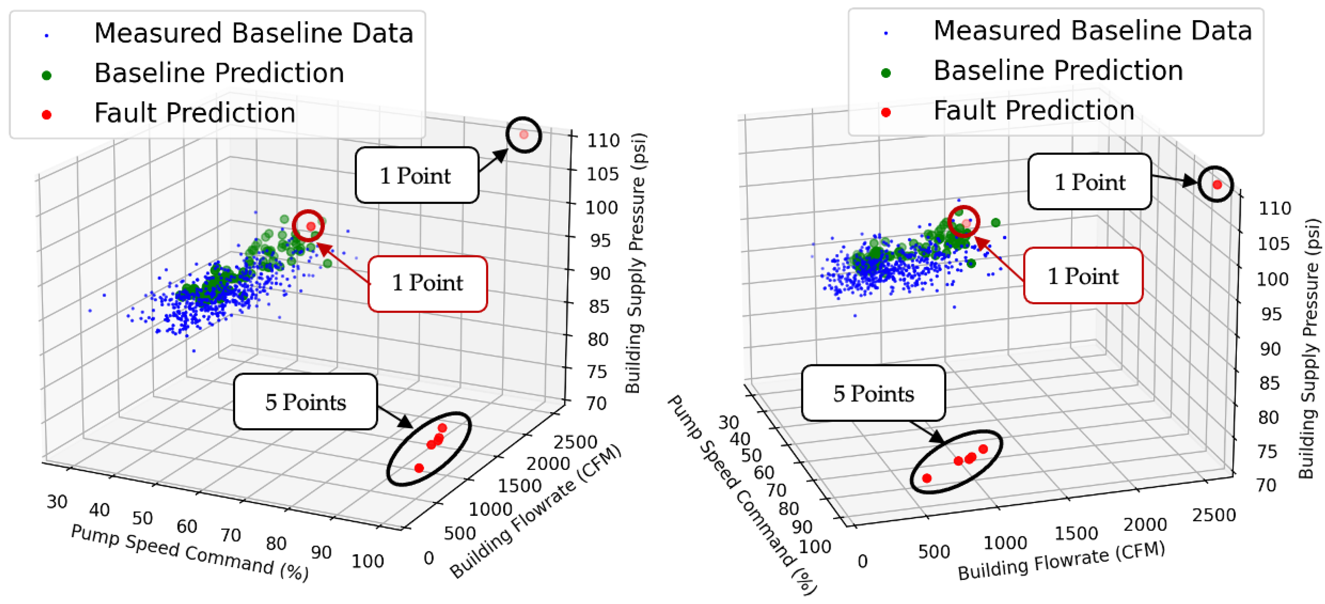
Additional testing data were measured from the system from the 1st to 3rd of October 2023. A fault representing a clogged strainer was introduced to the system manually by partially closing a shutoff valve, reducing flow through the pipes similar to the effect of a clogged strainer. The shutoff valve was closed until the chilled water pumps reached 100% command. This physical test was performed twice on 2 October 2023: once between 10:20 A.M. and 11:20 A.M. and a second time between 2:41 P.M. and 3:10 P.M. The duration of the tests were minimized to reduce the impact on occupants using the building for lectures and lab work. The measured data points from during the two tests are shown in Figure 8, circled in black.

Figure 9 plots the testing data alongside the baseline data. When the testing data were analyzed by an ML algorithm trained with the dataset shown in Figure 7, the algorithm classified 4% of the training points as faulty. This can also be described as a fault detection rate of 4%. The 4% fault detection rate is small due to the short duration of the introduced fault in the Zachry system, during which time only six points were measured. One additional point was measured at the beginning of the physical test before the system had reached its peak response, bringing the total number of faulty points in the dataset to seven.

The six points measured during the peak of the physical test are circled in black in Figure 8 and Figure 9. The point measured from the system at the beginning of the test, before the system’s peak response, is circled in red on Figure 9. The timestamp of this point was 10:30 AM on 2 October 2023 and is shown on Figure 8 by a vertical red bar. Figure 9 shows two views of the same data to clarify the location of the point circled in red. All seven points were classified as faulty by the model. The model made seven fault classifications and only detected the faulty points, yielding a prediction accuracy of 100%.

The testing data used in this example are the result of the testing procedure, which required a partially closed shutoff valve in the chilled water pipe. While immediate clogging may be expected if a large piece of debris becomes caught in the strainer, a more common scenario is that the strainer gradually becomes clogged with smaller pieces of debris.

In the case of gradual clogging, the system measurements shown in Figure 8 would drift toward their peak values over a period of weeks or months rather than within an hour. In contrast to the immediate clogging scenario shown in Figure 9, the data points measured during gradual clogging would produce a series of points originating from the cloud of measured baseline data points and terminating near the cloud of five fault prediction points.

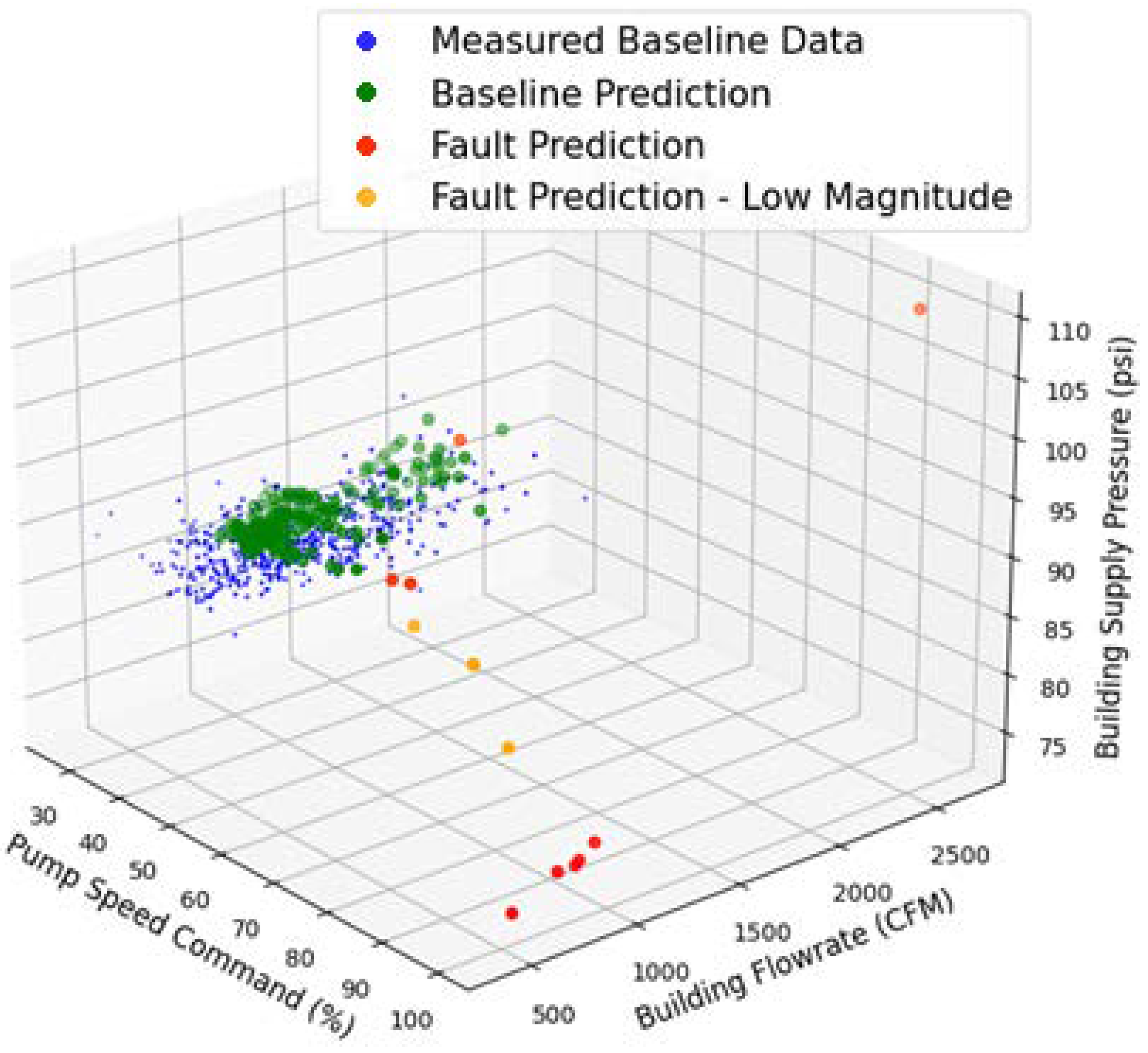
To determine the model’s ability to detect gradual clogging in the system, the machine learning model was tested using an additional dataset. The modified data used in the additional test consist of three data points which have feature values between the cloud of measured baseline data points and the five fault prediction points. These points represent gradual clogging in the system pipes.

The value of each simulated point is tabulated in

Table 1. Values of the progressively clogging strainer in Zachry’s CHW system.

Data Point	Campus Supply Pressure	Pump Speed Command	Primary Chilled Water Flow Rate	Building Supply Pressure
Baseline	73.9	64	1183.7	97.6
Progressive Fault 1	75	75	900	90
Progressive Fault 2	75	80	800	87
Progressive Fault 3	75	90	700	83
Peak Fault Value	75.7	100	551.6	73.3

. Each progressive fault point in Table 1 represents a progressive clogging of the strainer. The objective of this test is to determine if the machine learning model correctly classifies the progressive fault points as faulty.

Figure 10 plots the original testing dataset, the three progressive fault points described in Table 1, and the baseline data. The figure shows that despite the lower fault severity compared to the peak fault value, the model correctly classified each of the progressive fault points as faulty. The model’s successful fault detection of the progressive fault points shows that ML can detect gradual clogging of the system at three different severities. While gradual clogging in the system can take severity levels other than those tested, the model’s detection of all progressive fault points in this test suggests that machine learning can detect gradual clogging in the system and preemptively notify building operators of system failures.

4.2. Case Study Conclusions

This section demonstrated the use of ML-based AFDD to detect a clogged chilled water strainer. The model was tested by manually introducing the fault into the building system by closing a shutoff valve in the pipe, restricting flow, and simulating a clogged strainer. The model was shown to successfully detect the severely clogged strainer. An additional dataset was generated, representing a gradually clogging strainer. The ML model was shown to detect the points measured at all three generated data points in the progressive fault dataset.

5. Enthalpy Recovery Wheel Slipping

The Zachry building houses nine pretreatment-outside air (PTOA) units, which each serve conditioned outdoor air (OA) to other AHUs in the facility. The PTOA units consist of an enthalpy recovery wheel (ERW), a heating coil, a cooling coil, a supply air fan, and an exhaust air fan. MERV 7 filters are installed in the exhaust air duct and MERV 13 filters are installed in the supply duct. The exhaust fan draws exhaust air from the building and forces it through the exhaust portion of the enthalpy wheel.

The enthalpy wheel analyzed in this section, in PTOA-06-02, is a Thermotech TF-182 MSP wheel constructed with aluminum and coated with a molecular sieve. Each segment of this wheel is 36 inches long with interior and exterior linings of G90 20GA galvanized steel and is insulated using R-13 2” foam. The wheel is designed to create a Δ17 °F (Δ9.1 °C) temperature drop while cooling the OA and a Δ46 °F (Δ25.6 °C) temperature increase while heating the OA.

The enthalpy wheel is controlled by outdoor air temperatures (OAT): when the OAT is greater than 60 °F (15.6 °C), the enthalpy wheel will run at 65% speed. When the OAT is less than 60 °F (15.6 °C) but greater than 50 °F (10 °C), the enthalpy wheel will be off. When the OAT is less than 50°F (10 °C), the wheel’s speed will be controlled to maintain a leaving air temperature (LAT) of 52 °F (11.1 °C). This wheel is controlled by temperatures instead of a combination of temperature and humidity measurements because of reliability concerns with humidity sensors.

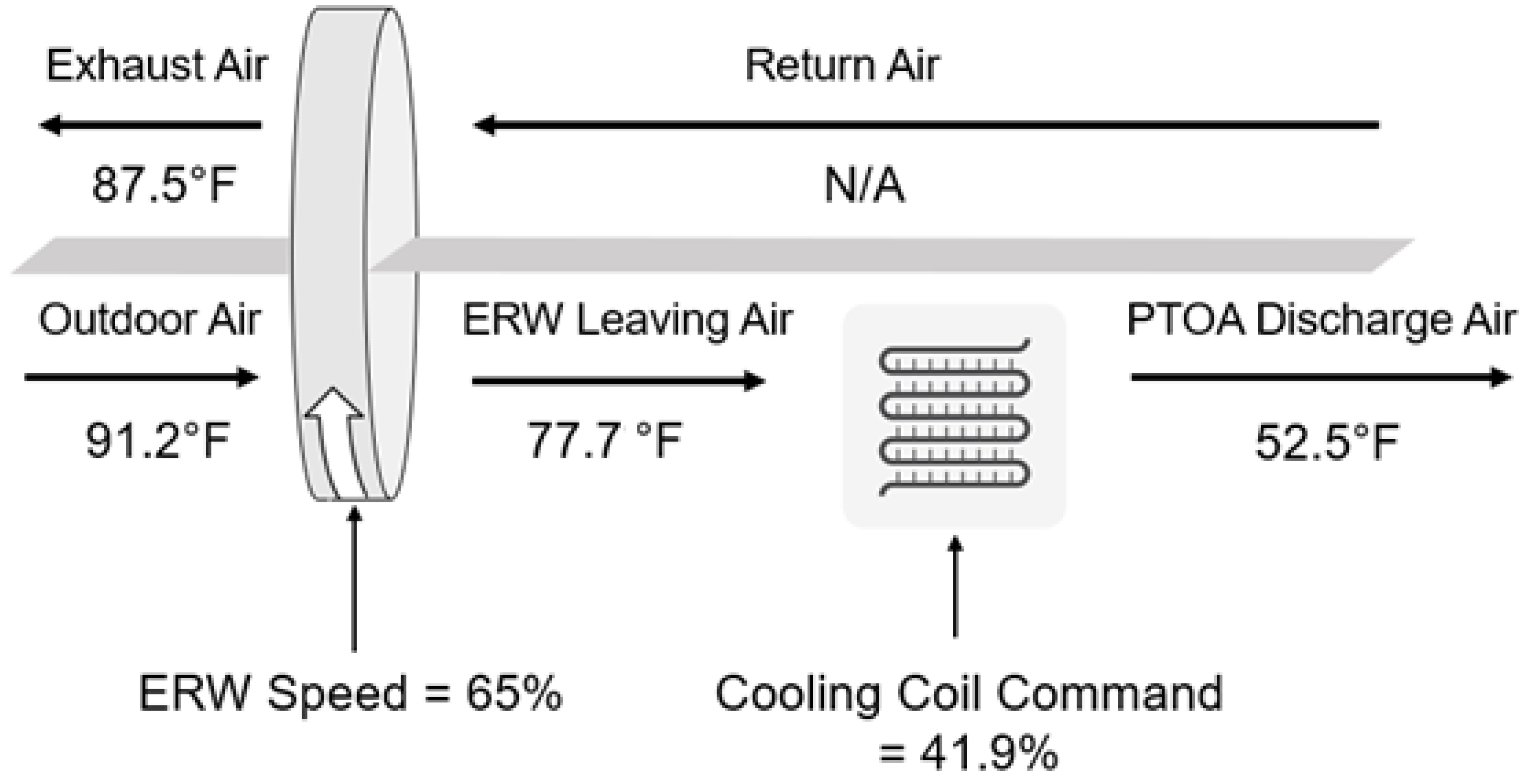
The cooling and heating coils are installed as secondary conditioning measures if the leaving air temperature of the ERW (ERW LAT) fails to meet the setpoint of 52 °F (11.1 °C). Consider the example shown in Figure 11, which displays values measured during cooling operation. The values shown in the figure were measured from PTOA-06-02 on 4 October 2023 at 2:30 PM. Return air temperature (RAT) is unmeasured. The OAT was 91.2 °F (50.7 °C). Because the OAT is greater than 60 °F (15.6 °C), the wheel’s motor is run at 65% speed command. The air leaving the wheel was 77.7 °F (25.4 °C), which is greater than the setpoint of 52 °F (11.1 °C). To condition the air to the 52 °F (11.1 °C) setpoint, the cooling coil engaged at 41.9% and produced a PTOA discharge air temperature of 52.5 °F (11.1 °C).

Ensuring that the PTOA DAT meets the temperature setpoint simplifies sequences of the successive AHUs, which can control discharge air temperatures without consideration of water content. The successive AHUs are also installed without hot water coils because the entering outdoor air temperature is expected to be 55 °F (12.8 °C), which simplifies maintenance and reduces the points of failure.

Sensors directly relevant to the ERW’s controls in cooling are entering OAT and enthalpy recovery wheel motor speed (ERW speed). In heating, the ERW LAT is used to control the rotational speed of the wheel and maintain an ERW LAT of 50 °F (10 °C). The temperature of the return air and supply air leaving the enthalpy wheel, as well as the flow rates of air through the intake and exhaust ducts, are also relevant to ERW performance. In this analysis, only temperature measurements are considered because those measurements are used to control the wheel.

The wheel’s true rotational speed is unmeasured. The wheel’s motor speed is used to calculate the rotational speed of the wheel, which is connected to the motor shaft by a fan belt. The wheel’s rotational speed relates to the motor speed according to the ratio of the circumferences of the motor and wheel pulleys. The wheel’s true rotational speed may differ from the design pulley ratio and the VFD speed command. As the wheel ages, the tension of the fan belt may decrease and cause the belt to slip.

Detecting a change in true rotational speed versus the design rotational speed at any given VFD speed command can lead to the detection of failures in the ERW. This situation can be difficult to detect using Boolean rules because the wheel’s true rotational speed is unmeasured. ML can perform rotational speed analysis by modeling the temperature difference across the ERW during each temperature range defined in the controls and detecting when the measured operation differs from the expectation. If the temperature difference across the wheel is lower than the expectation, the fan belt is likely slipping.

5.1. Case Study in Zachry

The baseline period for this analysis, defined based on normal wheel operations, is between 1 January and 1 October 2022. The baseline period is normally suggested to be at least one full year to reduce model bias toward certain outdoor air conditions but fault-free data exist only during a partial-year period for this PTOA unit. Because the model was trained without data from October to December, the model may have a bias against colder outdoor air temperatures and future analysis during those periods may produce unexpected results. To account for the missing winter data, the testing dataset for the wheel’s analysis was measured during summer months which were included in the baseline dataset. The baseline data are plotted in Figure 12, which shows that 91% of points are at either 0% or 65% ERW speed. Furthermore, 8.4% of the remaining 9% are at less than 10% ERW speed.

5.1.1. Fault Simulation

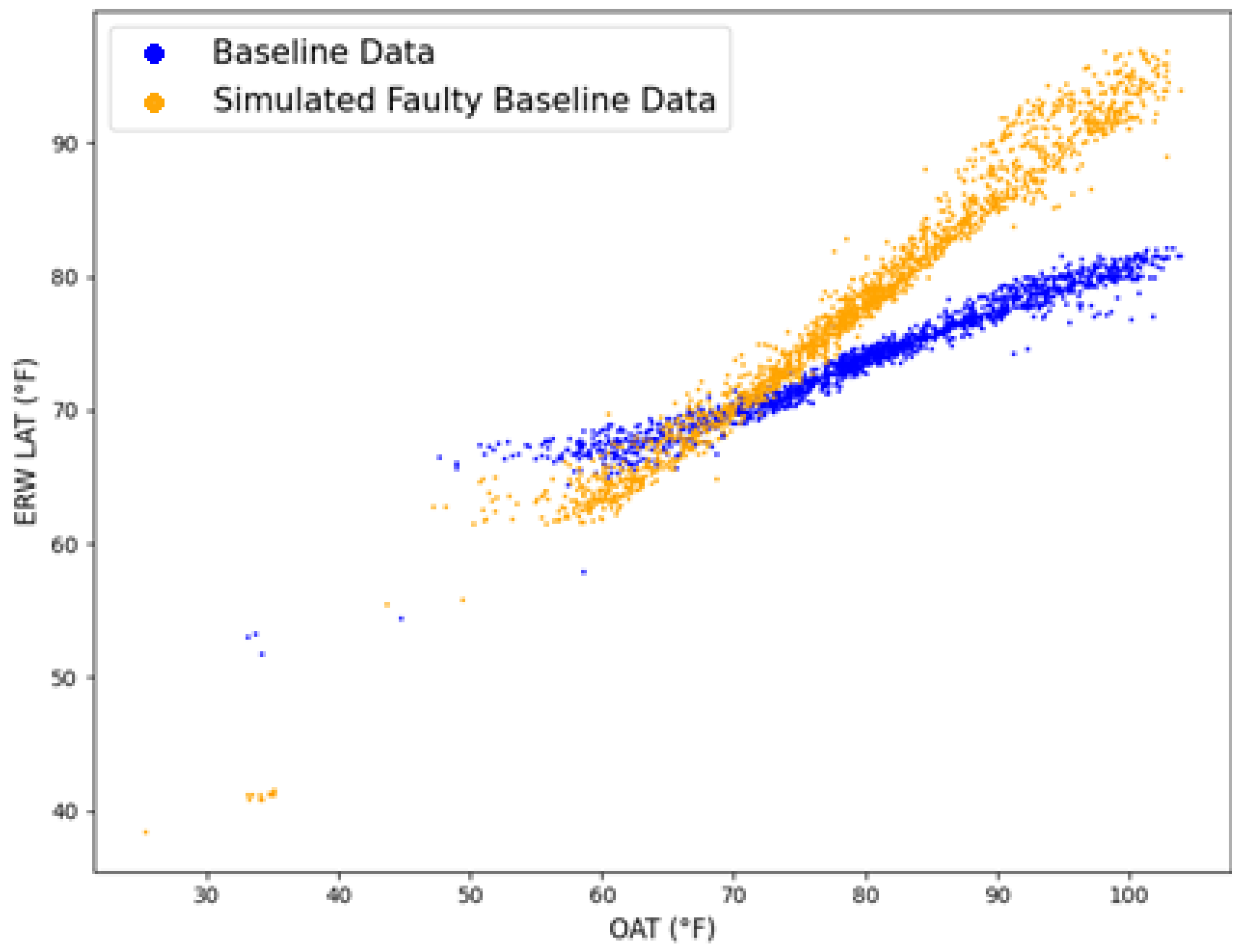
Slipping enthalpy wheels can be detected by an increased correlation between OAT and ERW LAT. As the wheel slips, the difference between OAT and ERW-LAT becomes smaller due to reduced energy transfer across the wheel. For this reason, the slipping enthalpy wheel is simulated using a trend value replacement method. The fault simulation halves the temperature difference across the wheel. For example, if the measured temperature difference across the wheel was 11.7 °F (OAT—ERW LAT = 88.2 °F–76.5 °F = 11.7 °F), the simulated fault modifies the wheel’s leaving air temperature to 82.35 °F so that the temperature difference across the faulty wheel is 5.85 °F (OAT—modified ERW LAT = 88.2 °F–82.35 °F = 5.85 °F). The simulation process is described further in previous work [3]. A plot showing the baseline data and simulated-faulty data at 100% ERW speed is shown in Figure 13.

5.1.2. Fault Detection

To compensate for the absence of low outdoor air temperatures in the defined baseline period, the analysis is performed using high outdoor air temperature data measured from 1 to 12 May 2023. During the testing period, the ERW speed was set to 65% when the OAT was above 60 °F. Figure 14 shows that the difference between ERW LAT and OAT is less than 3 °F in 78% of points and is less than 5°F in all but two points (99.7%). In the baseline period, the temperature difference was as high as 18 °F. The wheel’s design condition at these temperatures states that the temperature difference between the ERW LAT and OAT should be approximately 11 °F. Because the actual temperature difference is less than the design temperature difference, it is likely that the wheel is slipping.

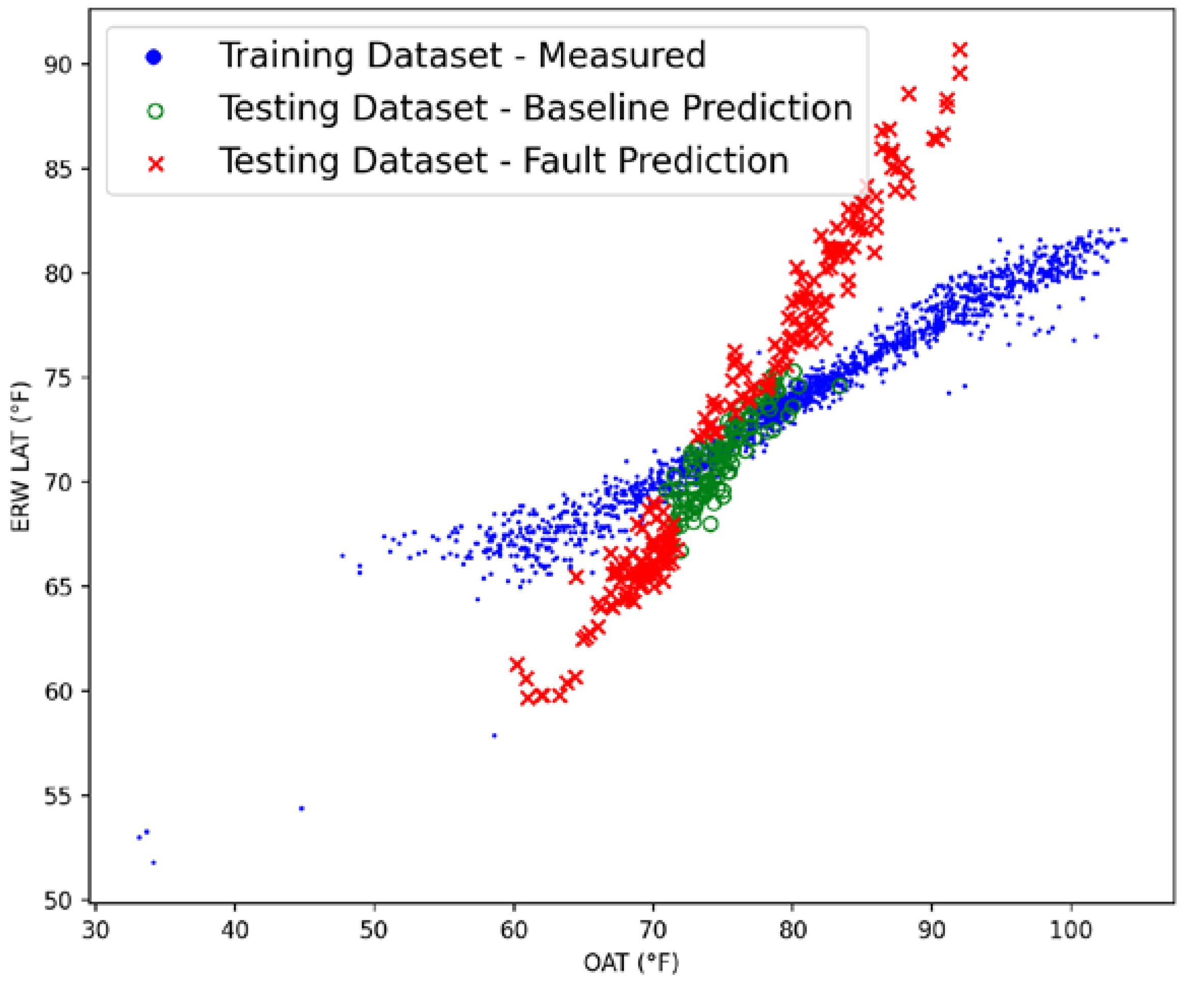
The testing data’s classification results using the trained ML model are shown in Figure 15, where the green and red points represent classifications made by the ML model in the testing period and the blue points represent data measured from the system during the baseline period. The ML model results show a fault detection rate of 60.4%. The two-dimensional plot contains points measured at 65% ERW speed. Figure 15 shows that as the data points in the testing period stray from the baseline points, they are classified as faulty (in red).

The relationship between ERW LAT and OAT measurements is expected during some system conditions. When the OAT and RAT in the system are equal or when the wheel’s motor speed command is 0%, the temperature difference across the ERW is expected to be 0 °F.

The classification results of Figure 15 show that ML can detect a slipping ERW based on temperature data, even though a direct measurement of the wheel’s rotational speed is missing.

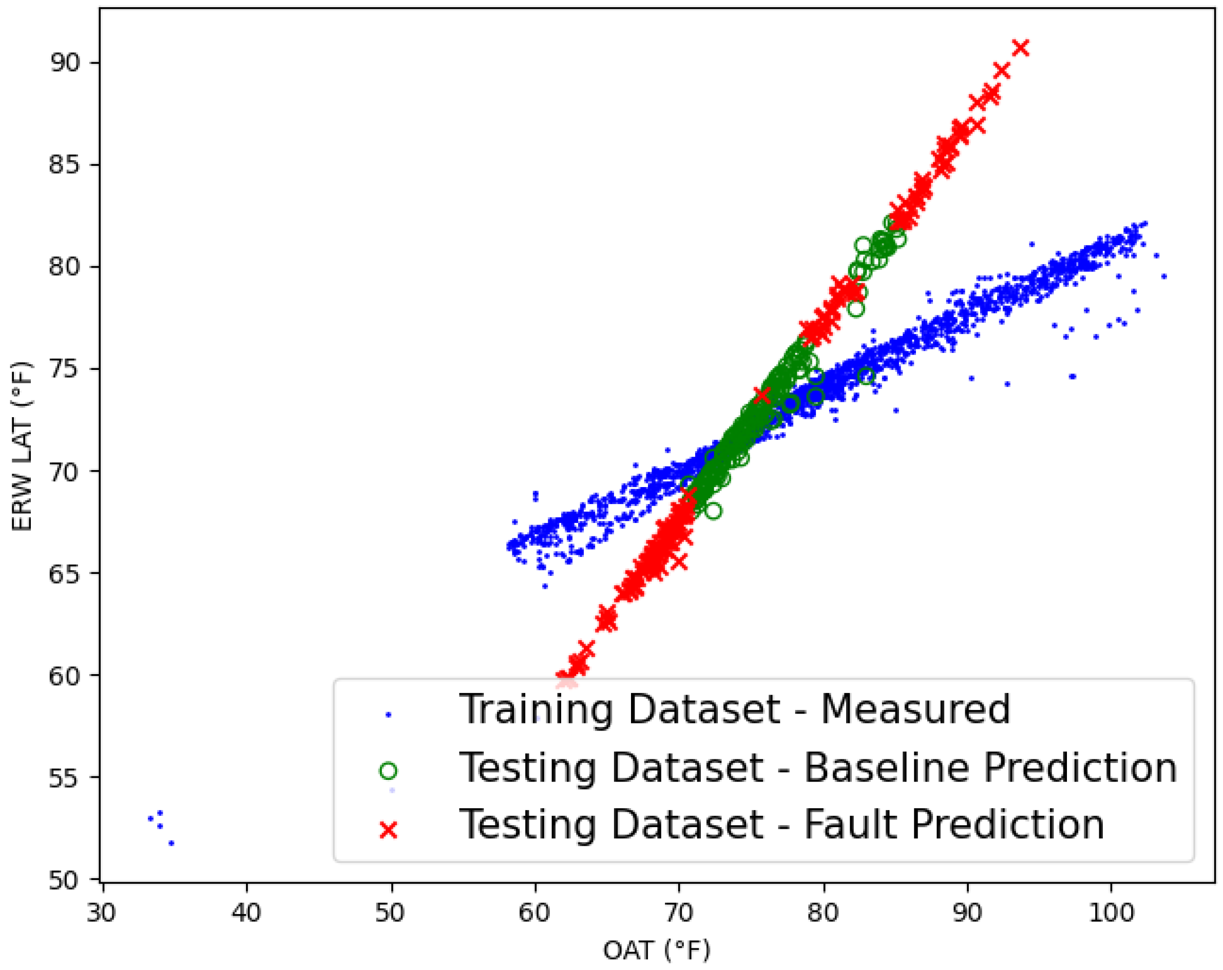
PTOA-06-02 is an enthalpy recovery wheel that transfers moisture between entering outdoor air and the system’s exhaust air. Moisture transfer can occur while temperatures are equal. Including humidity measurements in the analysis will allow the model to quantify all energy transfer across the wheel instead of relying solely on temperature differences, which can improve the model’s performance while the OAT and ERW LAT are equal. Results of the analysis when the humidity transfer across the wheel is included as a feature of the model are shown in Figure 16.

5.2. Case Study Conclusions

This section demonstrated the use of ML-based AFDD to detect a slipping enthalpy recovery wheel. The ML model was trained to estimate the energy transfer across the wheel while spinning as expected. The ML model detects lower-than-expected energy transfer and attributes the losses to a slipping wheel. An additional model was trained, which includes humidity measurements in the model’s features. Differences between the models are most pronounced while the ERW LAT and OAT are approximately equal.

6. Low Temperature Alarm

Anomaly detection models detect outliers in system operation but require manual analysis for diagnostics. Anomaly detection models may be preferred over classification models because of their relative simplicity to configure. Where classification models require a defined fault simulation (described in Section 4.1.4 and Section 5.1.1), anomaly detection models require only a defined list of model inputs (features). However, where classification models provide automated fault diagnostics, anomaly detection models require manual diagnostics after the fault has been detected.

For this research, a low-temperature alarm (LTA) event was triggered by the system and the alarm status was withheld from the dataset used to train an ML model. The ML model was trained to detect when either the preheat coil leaving air temperature falls below 35°F or when the system shuts down in response to the low-temperature alarm. The model serves as a backup to the freeze stat alarm, which may fail in two ways: the alarm may fail to announce the event or the alarm may fail to shut down the system. If the freeze stat alarm fails to announce the event or if the alarm fails to shut down the system, the ML model will detect the event and notify the operator.

There are other system failures that can use a trained ML model as a failsafe to diagnose and announce the problem. ML-based sensor failure or drifting detection can also improve the fault detection for humidity sensors, flow sensors, or temperature sensors.

6.1. Manual Diagnostics of a Low-Temperature Alarm Event

An anomaly detection ML model was trained using a baseline dataset measured from the Zachry system between 1 January 2022 and 1 January 2023. The dataset consists of 34,364 data points with three features: outdoor air flow rate through the PTOA-06-02 unit and the outdoor air flow rate through AHU-6-04 and AHU-6-05, which are AHUs supplied with preconditioned air from PTOA-06-02. The flow rate to the AHUs from PTOA-06-02 is measured with an Ebtron Gold Series Flow Meter, which is an electronic flow meter that measures flow in units of feet per minute in the ductwork and then calculates cubic feet per minute (CFM) in the control system.

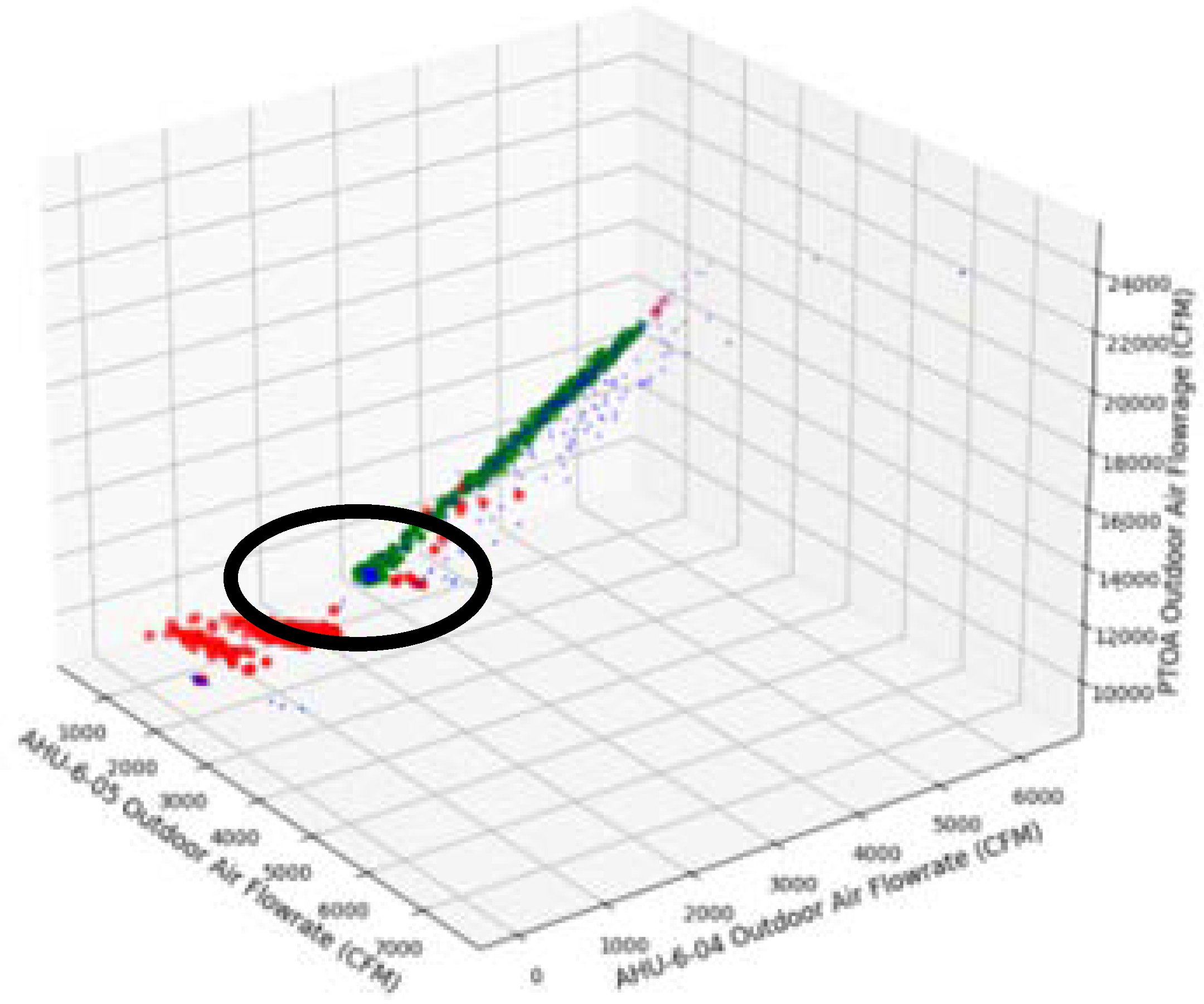
A testing dataset was measured between 15 February 2023 and 7 March 2023. The prediction results from a model trained using the baseline dataset are shown in Figure 17, where blue points represent measured data from the baseline period, green points are fault-free classifications from the testing period, and red points are faulty classifications from the testing period.

In Figure 17, a cloud of faulty predictions exists at low flow rates of all three units, shown by the points circled in black. The blue baseline points were included in Figure 17 to show the system’s behavior throughout the baseline period. Because there is an absence of blue baseline points within the black circle, that system behavior shows that an issue exists which needs to be investigated.

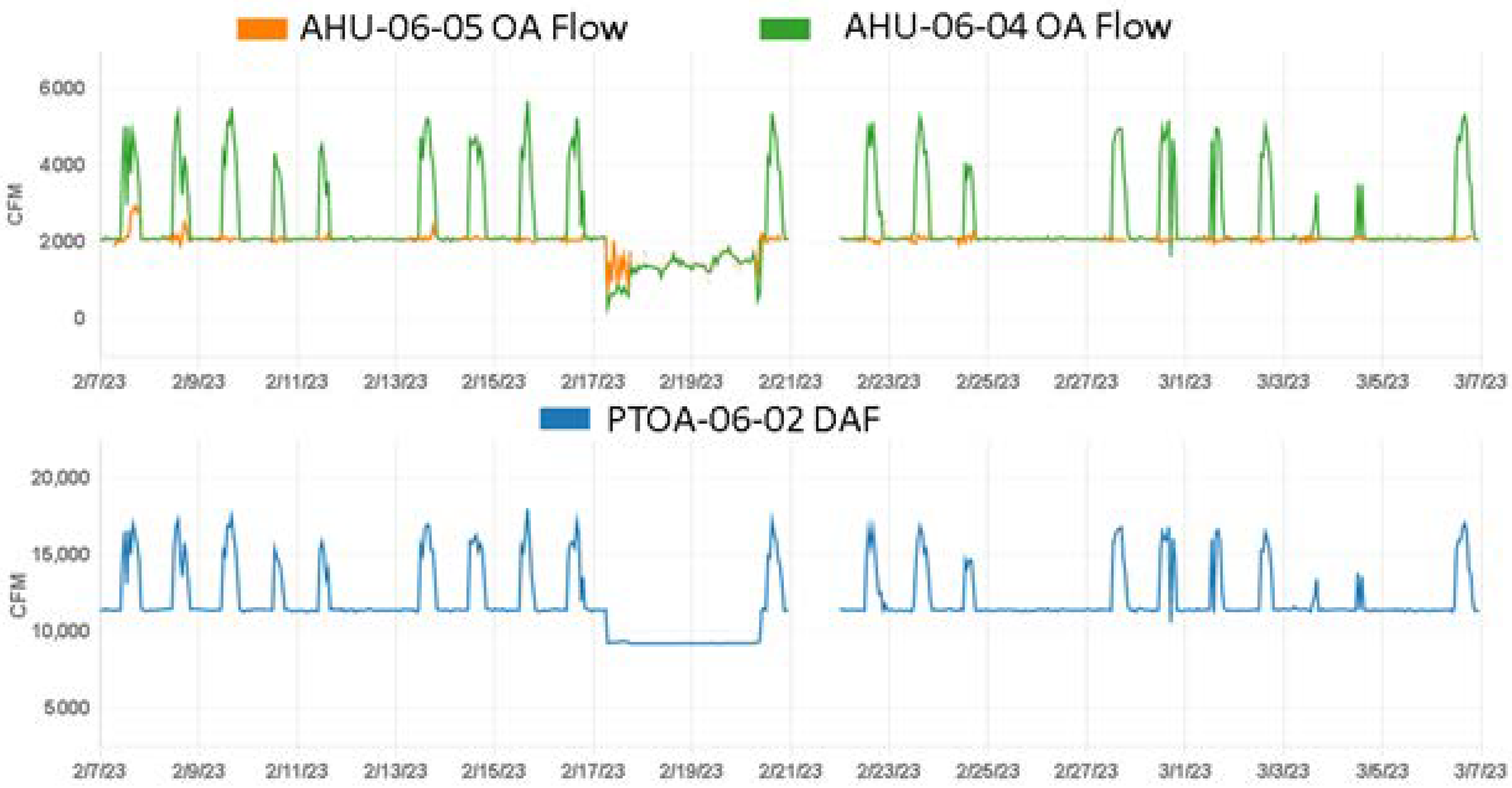
All points in the faulty data cloud, circled in black in Figure 17, were measured between 17 February 2023 at 12:15 A.M. and 20 February 2023 at 3:00 P.M. When the three features are plotted on a time series plot, the faulty behavior is visible as shown in Figure 18, which shows a period of abnormal behavior (a drop in airflow of approximately 2000 CFM [0.94 m³/s] in the PTOA unit and approximately 500 CFM [0.24 m³/s] in AHUs 06-04 and 06-05) between the time periods mentioned previously.

In the Zachry building, a freeze stat is installed on the discharge side of each preheat coil in PTOA units which, when detecting a drop in preheat temperature to below 35 degrees Fahrenheit, will de-energize all AHU fans, command the preheat and cooling coil valves fully open, and close the outdoor and exhaust air dampers. This is called a low temperature alarm (LTA) event. The de-energization of AHU fans caused by the freeze stat response is one possible cause for the decreased airflow through the system.

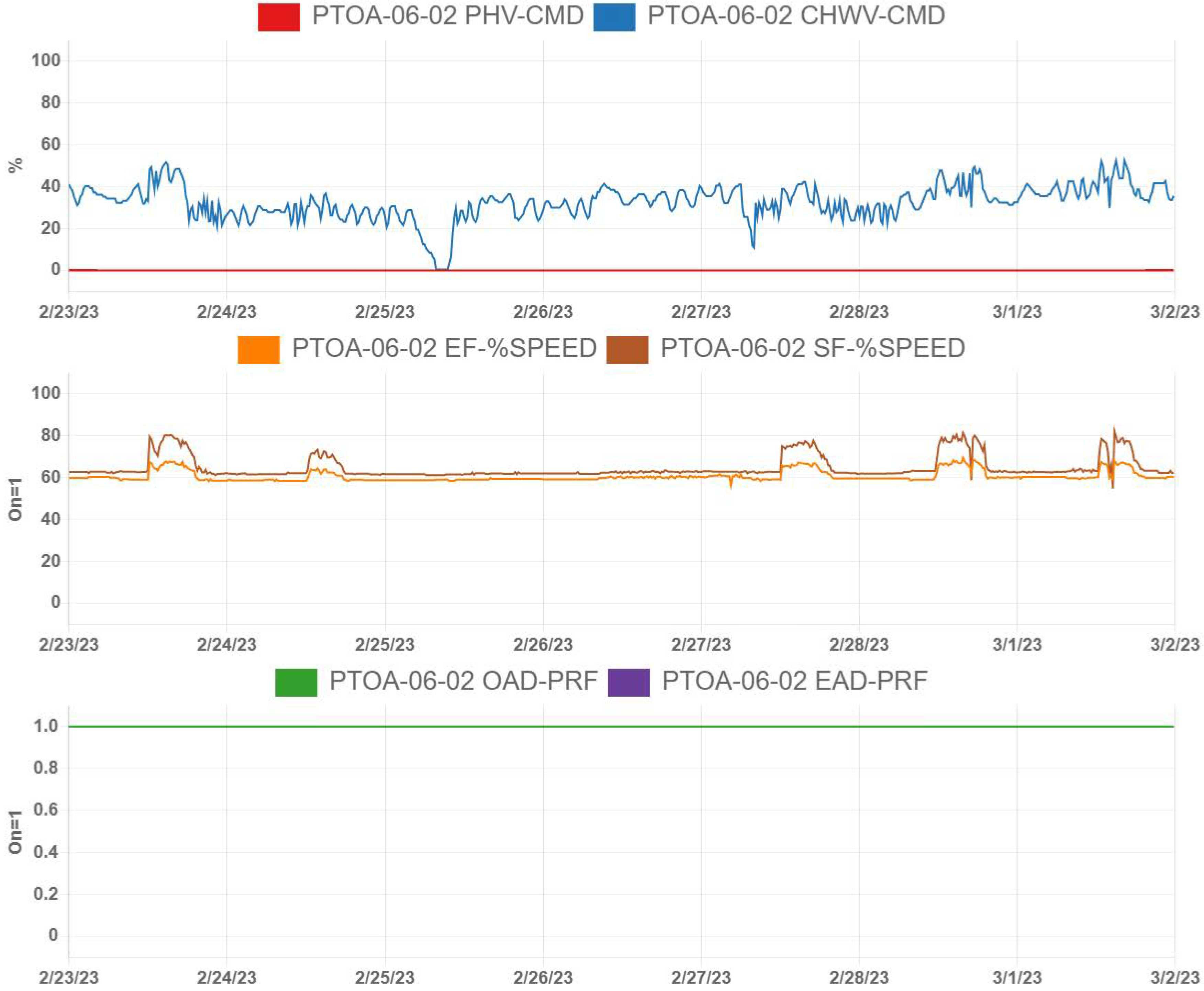
The PTOA fan speeds, coil commands, and damper positions are plotted in Figure 19. Notably, the bottom subplot, the PTOA-06-02 EAD-PRF series, is hidden by the PTOA-06-02 OAD-PRF series because the two series overlap.

Figure 19 confirms that the system is acting in response to the freeze stat alarm by meeting all six of the low-temperature alarm (LTA) response patterns described previously. Though the initial diagnostics of this fault required expert knowledge to confirm the original cause of the faulty behavior, the LTA response patterns can be used to train a classification model to perform automated detection and diagnostics of any future LTA event.

6.1.1. Developing a Diagnostic ML Model

The diagnostic model was trained with a dataset including simulated faults in a baseline dataset according to the freeze stat’s LTA response control definition:

• Supply and exhaust fan speed measurements are overwritten to be 0%, simulating offline fans;
• Preheat and cooling coil command measurements are overwritten to be 100%, simulating maxed out coils;
• Outdoor and exhaust air damper commands are overwritten to be 0%, simulating closed dampers.

The trained model learned to detect these behaviors and diagnose the period as an LTA event. When the model evaluated data measured between 16 February 2023 and 23 February 2023, its low-temperature alarm predictions aligned with the LTA event measured from the building between 17 February 2023 at 6:11 A.M. and 20 February 2023 at 9:00 A.M. The prediction accuracy of the model is 100%. The reason for the model’s perfect prediction accuracy is the LTA response pattern, which commands six components to a defined constant value. The response is predictable, reproducible, and distinguishable from normal operation, as seen in Figure 19.

6.1.2. Incomplete System Response

Because of the static event response pattern, a Boolean rule-based FDD analysis would also be capable of detecting and diagnosing the fault with the same perfect accuracy. However, Boolean rule-based analysis is unable to detect the fault if just one response fails to meet the rule’s threshold. ML resolves this problem by defining decision boundaries on a probabilistic scale and can detect the fault even with the missing measurement.

It is possible that, due to a hardware malfunction or existing fault, the system responds to the freeze stat alarm with only five of the six expected commands. If only five of six system responses are measured, a rule-based system will classify all points as fault-free due to incomplete rule matching. The ML algorithm trained in Section 6.1.1 correctly classified points within the LTA event when up to two of the six freeze stat responses were missing.

6.1.3. Validation Plot

Figure 19 plots the six freeze stat response variables during the LTA event. Figure 20 plots the six freeze stat response variables during normal operation. Notably, as seen in Figure 19, the PTOA-06-02 EAD-PRF series is hidden by the PTOA-06-02 OAD PRF series because both series values equal 1 for all timestamps. When an LTA event is detected in the system, the building operator will be notified of the detection and automatically be provided with the plot of the freeze stat response variables.

Building operators can compare normal operation, shown in Figure 20, to the data measured during a detected LTA event, shown in Figure 19, to verify the fault detection. Because the PTOA unit uses 100% outdoor air, the outdoor air damper remains open at all times. Outdoor air flow rate modulation is controlled by the outdoor air dampers of AHU-06-04 and AHU-06-05, which receive preconditioned outdoor air from the PTOA unit. Using ML for this analysis enables the building operator to train a model that detects LTA events in the building under more system conditions than a rule-based FDD system allows and automatically provides the operator with time series plots to verify the fault.

6.2. Case Study Conclusions

This section demonstrated the use of ML-based AFDD to detect LTA events in building systems. While the original anomaly detection model was able to detect anomalous behavior in the building, expert knowledge was required to define a ML model to diagnose the detected behavior. Future work may explore the ability of ML to automatically diagnose anomalous behaviors based on building control sequences. The sequences, which exist as part of the mechanical schedules of the building, could be used as features in the model for a more automated diagnostic procedure.

7. Conclusions

This paper defined a generalized data preprocessing procedure making use of standardized dataset definitions and point organization which allows one dataset definition to be applied across different projects for scalable ML analysis. The paper also presented three examples of applied ML to building systems on the Texas A&M University campus in College Station, Texas. Each example was designed to showcase a specific effect of using ML analysis for AFDD in building systems.

The first example analyzed chilled water pump data. A fault was manually introduced in the testing period by closing a manual valve which restricts the chilled water flow rate through the pipes. ML analysis was able to detect 100% of the faulty points. Additional analysis was performed, which analyzed the fault at progressive levels to verify that ML can preemptively detect failures in the system, allowing operators to resolve the fault before it has a negative impact on system operation.

The second example analyzed one of Zachry’s enthalpy recovery wheels. The model was trained to detect when the energy transfer across the wheel differs from the expected transfer according to the wheel’s motor speed, caused by a slipping wheel. The model learned to calculate the expected transfer across the wheel by modeling the energy transfer across the wheel during the baseline period. When trained with a full year of baseline data, the model was able to successfully detect when the wheel was slipping.

The third example analyzed low temperature alarms in the system. A model was trained using one year of data from the Zachry system. An evaluation period was defined and analyzed, which produced a fault detection rate of 23.9%. Deeper analysis was conducted to investigate the time period during which the faulty points were measured and a diagnostic ML model was developed for future fault detections. A faulty low temperature alarm was detected and confirmed via autogenerated time series plots.

8. Future Work

Section 6 of this paper discussed misclassifications produced by ML models. The suggested resolutions of misclassified points rely on manual input by building operators to further calibrate the model. Future work should focus on both minimizing the number of misclassified points by ML models and minimizing the amount of manual input required to resolve the remaining misclassified points.

The research described in this paper focuses on data measured from the building management system. Data preprocessing for the analysis consists of standardized fault simulation which expands the feature space to detect faulty behavior. While the results of the analysis show that faults can be detected, the simulated faults are estimations of what faulty behavior might look like in the building based on an understanding of the energy flow through the system.

An alternative data preprocessing approach would be to utilize feedback from building operators who are familiar with the building and its common failure modes. Rather than simulating faulty behavior based on first-principles equations as an estimate of how the building will respond to equipment failure, the building operators can manually define faulty time periods and describe the fault occurring in that period. Engineers can use this information to train diagnostic ML models. This process serves as data labeling for classification analysis and will expand the preconfigured knowledge to expose more faults to the operator. An example of the data labeling process is shown in Section 6.

The ML algorithm will search for failures similar to those defined in the diagnostic models. This can provide an analysis that is specific to the building instead of a generalized estimation of faulty behavior in buildings. As building operators work with engineers to define more faulty behaviors, the algorithm’s search space expands and becomes more informative. ML will gain more knowledge of the building and its failure modes to make personalized predictions and analyses as building operators use the tool and label system faults.