CFD Investigation of the Hydraulic Short-Circuit Mode in the FMHL/FMHL+ Pumped Storage Power Plant

Abstract

The flexibility of the FMHL+ pumped storage power plants can be improved by extending the hydraulic short-circuit operating mode. CFD simulations of the flow in three bifurcations are performed to calculate the head losses and to investigate the flow topology in the pipes. A specific attention is paid to the influence of the curvature correction that has been developed for two-equation RANS turbulence models. For the T-junction considered, the activation of the curvature correction influences the head losses whereas for the two Y-junctions computed, no effect is observed. By comparing with the Y-junctions, the T-junction leads to higher head losses and helicity in the pipes downstream of the bifurcation. Compared to the current the intragroup hydraulic short circuit operation permitted, the intergroup and interplant hydraulic short circuit mode should provide better performances with possible gains until of −55% in head losses and −94% in helicity upstream of the turbines.

1. Introduction

The development of wind and solar energies, which are stochastic energies, requires increasing the amount of available flexible sources of energy production and storage to manage grid balancing. Pumped-storage hydro power plants (PSP) are the only matured solution for a large-scale electrical storage capacity based on a renewable energy source [1]. In 2014, the installed PSP capacity exceeded 150 GW around the world and represents almost 99% of the world’s current large-scale electricity storage [1]. Through Europe, some new PSP have been built for twenty years such as Kops II (Austria) [2], Linth-Limmern (Switzerland) or Nant-de-Drance (Switzerland). Extension of existing PSP has also been achieved as is the case for the Forces Motrices Hongrin-Léman (FMHL, Switzerland) within the project FMHL+ [3]. In turbine mode, PSP can provide a large power flexibility thank to the use of discharge governor such as guide vanes or needles. However, in pumping mode, their flexibility is often limited due to the fixed operating point of the pump(s). To add flexibility also in pumping mode, two solutions can be considered: variable speed motor-generators or hydraulic short-circuit (HSC) mode. The HSC operating mode consists in operating the pump(s) and the turbine(s) at the same time, allowing the adjustment of the energy consumed by the pump(s) with respect to the grid. Therefore, it becomes possible to provide system services such as frequency containment reserve or frequency restoration reserve also in pumping mode. This point is demonstrated in [4], where the authors show the contribution of a hydraulic short-circuit pumped-storage power plant to the load frequency regulation (LFR) of an isolated power system. The HSC mode is already used in several power plants such as Kops II (Austria) [2], Säckingen (Germany) and FMHL+ (Switzerland) [3] and is in demonstration at Grand’Maison (France) in the framework of the XFLEX HYDRO H2020 European project [5]. At Grand’Maison, the HSC mode is now considered as a third mode with 2500 h of operation in less than 2 years, which corresponds to 50% of the time where the pumps are in operation.

Few publications paid attention to the study of the bifurcations in the field of pumped-storage operations. Huber et al. [6] focuses on the flow in a T-junction by performing both model tests and CFD simulations. A good agreement is noticed between the measurements and the CFD results except for the case with a discharge from the reservoir higher than the one from the pump. In [7], the authors focuses on the head losses in the junction (bifurcations and trifurcation) of the Grand’Maison power plant by performing CFD simulations. The use of different software, meshes, RANS turbulence models shows the influence of the turbulence model for specific flow configurations in Y-junction. The RNG k-$ϵ$ turbulence tends to predict higher losses than the realizable k-$ϵ$ and SST turbulence models.

Among various objectives, the HydroLEAP research project [8] focuses on the extension of the HSC mode for the FMHL/FMHL+ PSP. Nowadays, the only HSC mode available is the intragroup one, for which the pump and the turbine of one group of the Veytaux 2 power plant can be operated between −114 MW to −35 MW (the negative sign refers to a power consumption regarding to the grid). The last power value corresponds to a HSC operation with a discharge in the Pelton turbine equal to 66% of its nominal value. For higher discharges, the jet quality decreases, which increases the risk of cavitation and therefore the erosion of the buckets. Consequently, it is not permitted to operate the turbine at a higher discharge in HSC mode. The project aims at extending this power range and investigating two other HSC modes: one between two groups of one power plant or another one between the two power plants. Since no experimental measurements are available, numerical simulations are the only way to compute the head losses and to investigate the flow topology in the bifurcations. Consequently, Reynolds-Averaged Navier-Stokes (RANS) simulations are performed using both the SST and BSL-EARSM turbulence models with a specific attention paid to the influence of the curvature correction terms since swirling flows develop in the pipes in HSC mode.

This paper is structured as follows: the FMHL/FMHL+ case study is presented in Section 2, Section 3 focuses on the meshes and the numerical setup, the results are presented separately in Section 4 for each bifurcation, before being compared in Section 5 and a conclusions is proposed in the last Section 6.

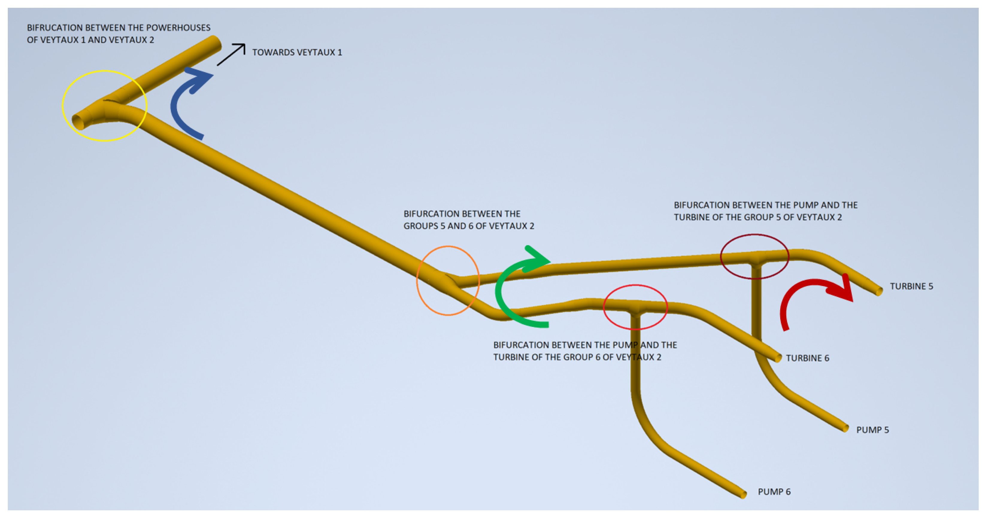
2. Description of the FMHL/FMHL+ Power Plant

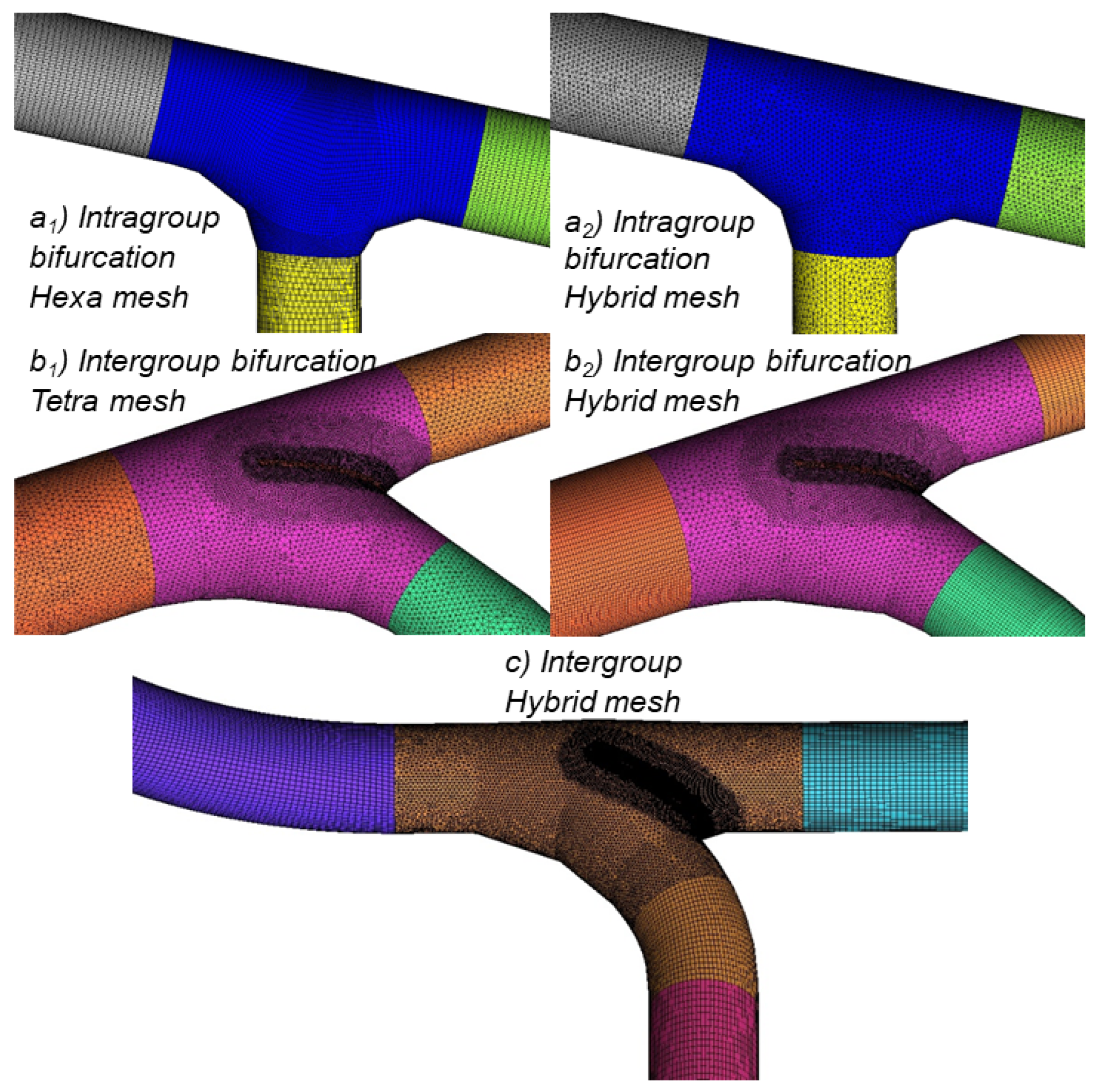
Originally, the FMHL power plant was a PSP plant located in Switzerland near Montreux between the reservoir of Hongrin and the Leman Lake in operation since 1971. The power plant features 4 horizontal ternary groups of 60 MW each consisting of two two-jet Pelton turbines and a five-stage centrifugal pump. During the last decade, a new power plant FMHL+ has been built near the previous one to double the available power. The new power plant features two vertical ternary groups (groups 5 and 6) of 120 MW each [3] consisting of a five-jet Pelton turbine and a five-stage centrifugal pump. The gross head is 883 m.

Considering the pipes of FMHL’s groups illustrated in Figure 1, the different variants of HSC modes are shown. The FMHL+ power plant was designed in such a way that a HSC mode is available inside the same group (called intragroup HSC mode), i.e., the pump and the turbine of the same group are operated at the same time (see the red arrow in Figure 1). However, the turbine power in this mode is limited to 66% of its maximum power. The HSC modes between the two groups of FMHL+ (named intergroup HSC mode and illustrated by the green arrow in Figure 1) and between the two power plants (interplant HSC mode, blue arrow in Figure 1) are for now not permitted. The extension of the intragroup HSC mode and the possibility of operating the intergroup and interplant HSC modes are among the main objectives of the HydroLEAP project to offer improved system services [8].

3. Numerical Setup

Based on the 3D geometry of the pipes shown in Figure 1, a computational domain for each HSC mode is considered (see Figure 2). The intragroup bifurcation looks like a T-junction whereas the intergroup and interplant bifurcations look like an asymmetric Y-junction with the presence of a reinforcement at the bifurcation, highlighted by a red arrow in Figure 2. The valve bodies along the pipes constitute the only simplification of the geometry. The bifurcations are faithful to the real power plant with diameters from 1600 to 2700 mm and pipe lengths from 10 to 30 m.

The meshes illustrated in Figure 3 were created with the software ICEM CFD™ version 2021 R2.

Table 1. Properties of the meshes.

	Intragroup Bifurcation		Intergroup Bifurcation		Interplant Bifurcation
Mesh type	Hexa	Tetra + prisms	Tetra + prisms	Hybrid Hexa/Tetra + prisms	Hybrid Hexa/Tetra + prisms
Max element size [mm]	100	100	150	150	150
Number of elements [millions]	6.36	8.19	5.64	2.01/2.11	1.45/3.11
Number of prisms layers [-]	-	30	20	-/15	-/12
Height of the first cell [mm]	0.01	0.01	1	1	1
Maximum y+ [-]	9	6	687	1034	719
Averaged y+ [-]	3	3	183	308	189
Averaged quality	0.96	0.92	0.89	0.93/0.87	0.96/0.87

summarises the mesh characteristics for each computational domain. For methodology reasons and to consolidate the mesh independence of the CFD results, two types of mesh were tested for the intragroup and intergroup bifurcations. This approach inspired by [9] is justified by the quantification of the uncertainty among the meshes.

The reinforcement (see the red arrows in Figure 2) at the intergroup and interplant bifurcations prevents the generation of a hexahedral mesh due to the presence of element with a too poor orthogonality. Therefore, hybrid meshes combining hexahedral meshes for the pipes and a tetrahedral mesh for the junction have been generated. The connections between the meshes are performed by numerical interfaces. The relatively high value for the average and maximum $y^{+}$ values (see Table 1) have been validated by comparing the head loss coefficients with the literature in a T-junction at 90 degrees [5]. Only the intragroup domain was meshed using $y^{+}$ value below 10 and a finer wall boundary resolution to better understand the dispersion of the results for this test case (see Section 4.1).

The simulations were set up and solved with Ansys^® CFX^® 2021 R2. The flow is modelled using the incompressible RANS equations [10]. The Reynolds stresses are computed using either the eddy-viscosity SST k-$\omega$ turbulence model [11] or the explicit algebraic Reynolds stress BSL-EARSM model [12]. For both turbulence models, the simulations have been performed with or without the activation of the curvature correction (CC) term that imposes a limiter on the production term of both k and $\omega$ for the SST k-$\omega$ model [13] or replaces the normalized mean flow rotation rate tensor by the effective mean flow rotation rate tensor for the BSL-EARSM model [14]. The influence of the curvature correction is considered in this paper since swirling flows are observed downstream the junction mainly for T-junctions. The boundary layer is modelled using an insensitive $y^{+}$ wall function [15]. A high-resolution numerical scheme is used for the advection term of the momentum equation, whereas for the turbulence equations, only a first-order scheme is specified in agreement with the recommendations in [16]. The set of equations is solved using a couple algorithm using a pseudo-time step for the iterative procedure. Steady state simulations are performed by achieving 1000 iterations and using the default values of the numerical parameters. The root mean square residual target value is set to ${10}^{-4}$ for all the variables, even if they stabilize between $2\times {10}^{-4}$ and $4\times {10}^{-4}$. Concerning the intragroup simulations, some regular oscillations on the monitors of the total pressure were noted, even if the simulation was converged regarding the residuals. These pseudo-steady results are considered as converged results. According to the arrows in Figure 4, the boundary conditions are set as follows:

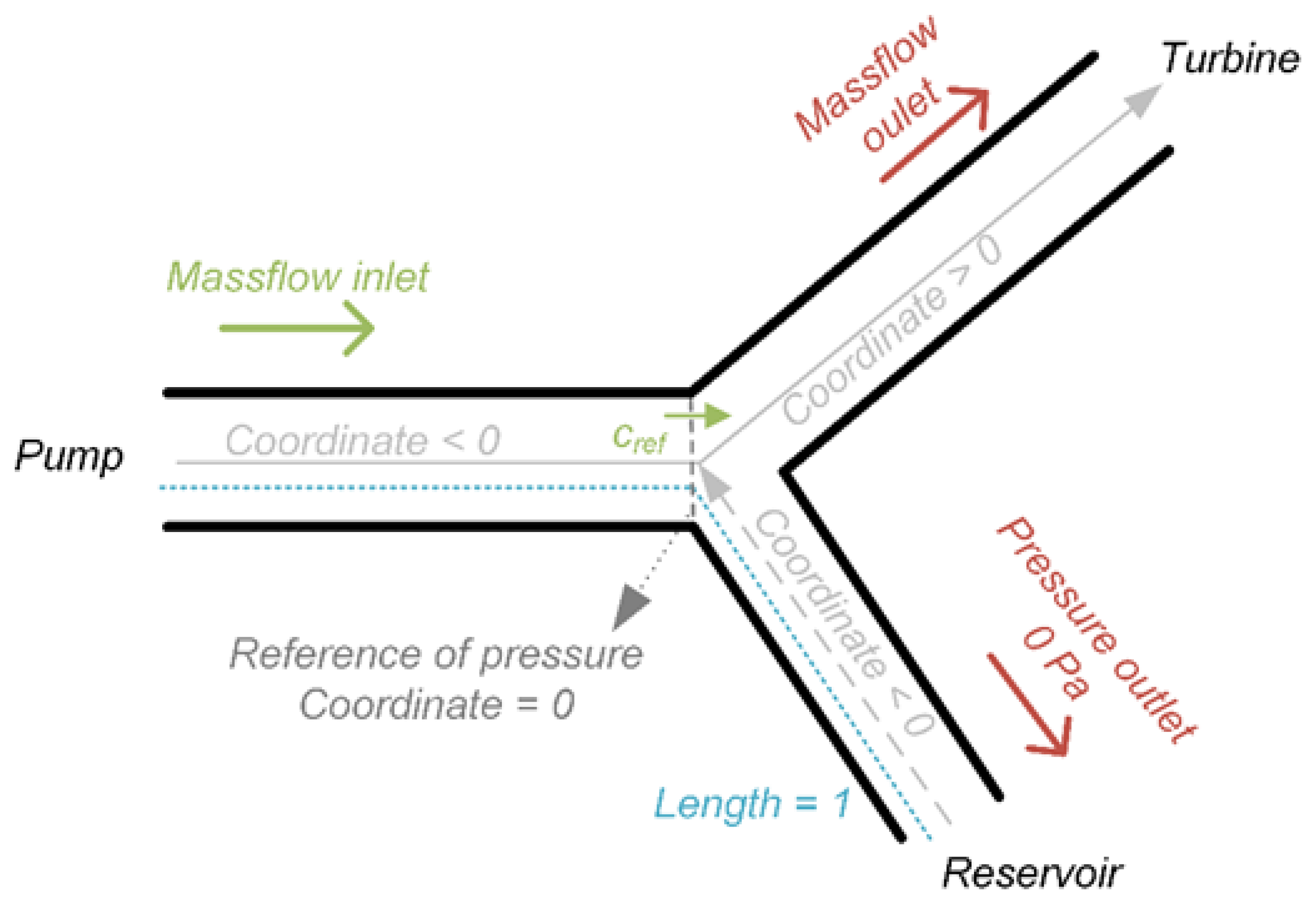
• At the inlet of the computational domain, i.e., at the pump side, the flow rate is imposed according to the operating point of the powerplant listed in the

  Table 2. Pumping flow rate and Reynolds number according to each HSC mode considered.

  Pumping Plant	Pumping Group	Intragroup	Intergroup		Interplant
  Veytaux II	Group 5	12.4	12.4		12.4	12.4
  	Group 6	12.4		12.4		12.4
  Veytaux I	Group 1						6.7	6.7	6.7	6.7
  	Group 2							6.7	6.7	6.7
  	Group 3								6.7	6.7
  	Group 4									6.7
  Pumping flow rate [m${}^{\mathbf{3}}$/s]		12.4	12.4	12.4	12.4	24.8	6.7	13.4	20.1	26.8
  Reynolds number [-]$·{\mathbf{10}}^{\mathbf{6}}$		110	$8.8$	$8.8$	$5.8$	$1.2$	3.2	$6.3$	$9.5$	130

  . The velocity profile is assumed uniform and the turbulent intensity is set to a default value of 5%.
• At the outlet section in the direction to the turbine, a mass flow rate is imposed to fix the percentage of the pumped flow deviated to the turbine, i.e., the percentage of HSC.
• At the outlet section in the direction of the upper reservoir, the static pressure is set except when the entire part of the pumped flow is deviated to the turbine (100% HSC mode). In this latter case, a free slip wall condition is imposed, and the pressure is specified at the outlet of the pipe in direction of the turbine.

Figure 4. Scheme of the boundary conditions on an arbitrary bifurcation within addition to the curvilinear coordinate frame used for the post-treatment of the results.

Figure 4. Scheme of the boundary conditions on an arbitrary bifurcation within addition to the curvilinear coordinate frame used for the post-treatment of the results.

Table 2 provides the flow rate pumped for each operating point considered. In the interplant column, the values in grey were not considered for the simulations, to save computational time. For each HSC configuration, four discharge ratios $Q_{turbine}/Q_{pump}$ are computed: 0% (pumping mode), 33%, 66% and 100% (all the discharge is deviated to the turbine).

4. Results and Analysis

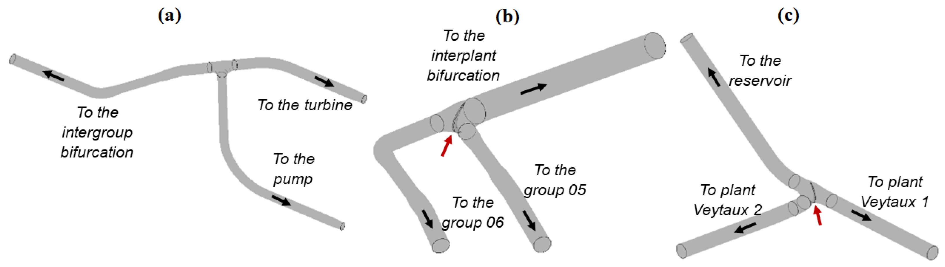
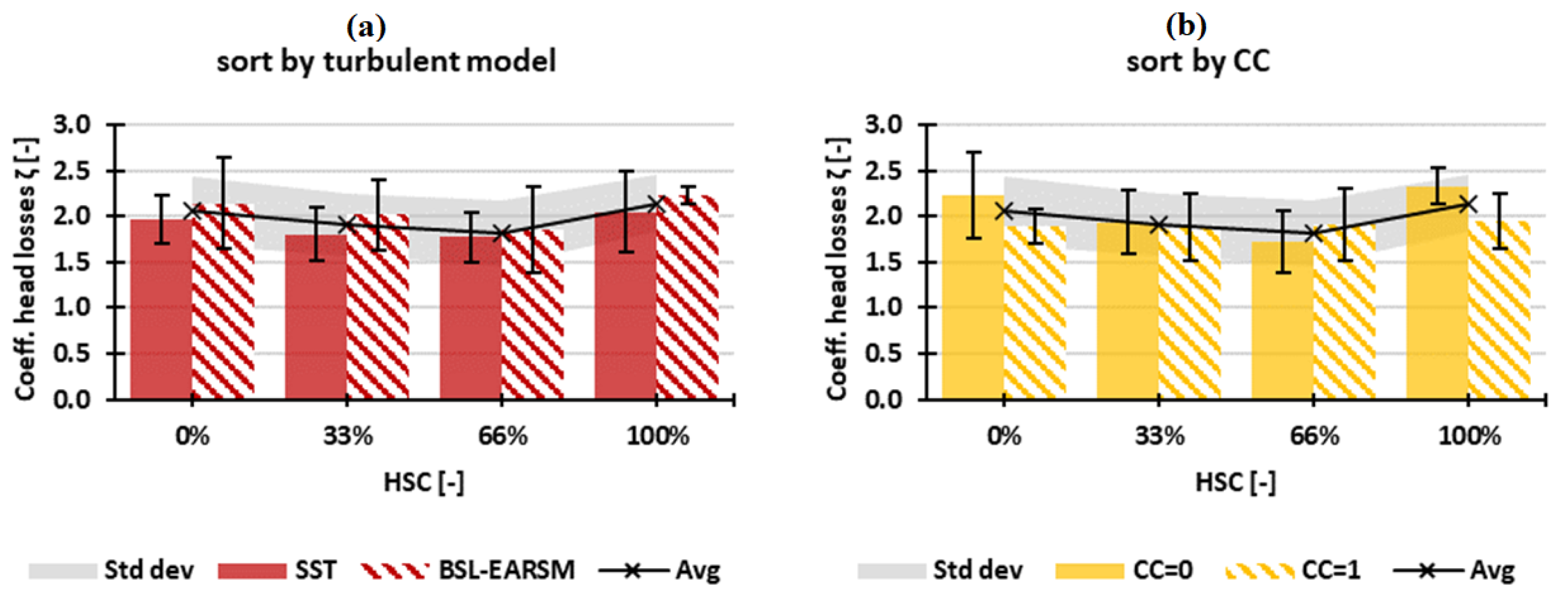
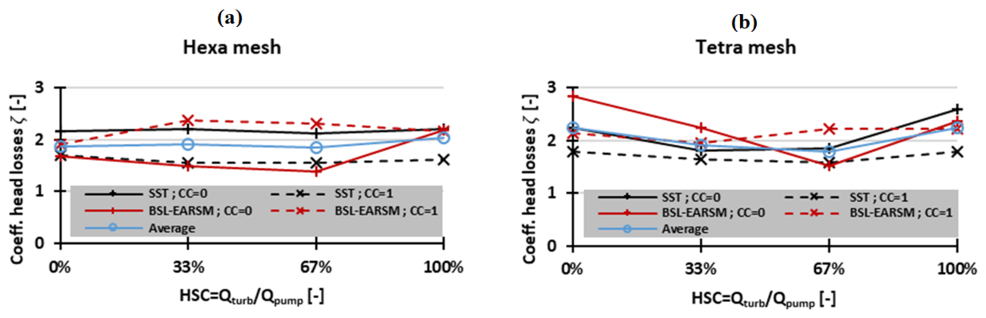
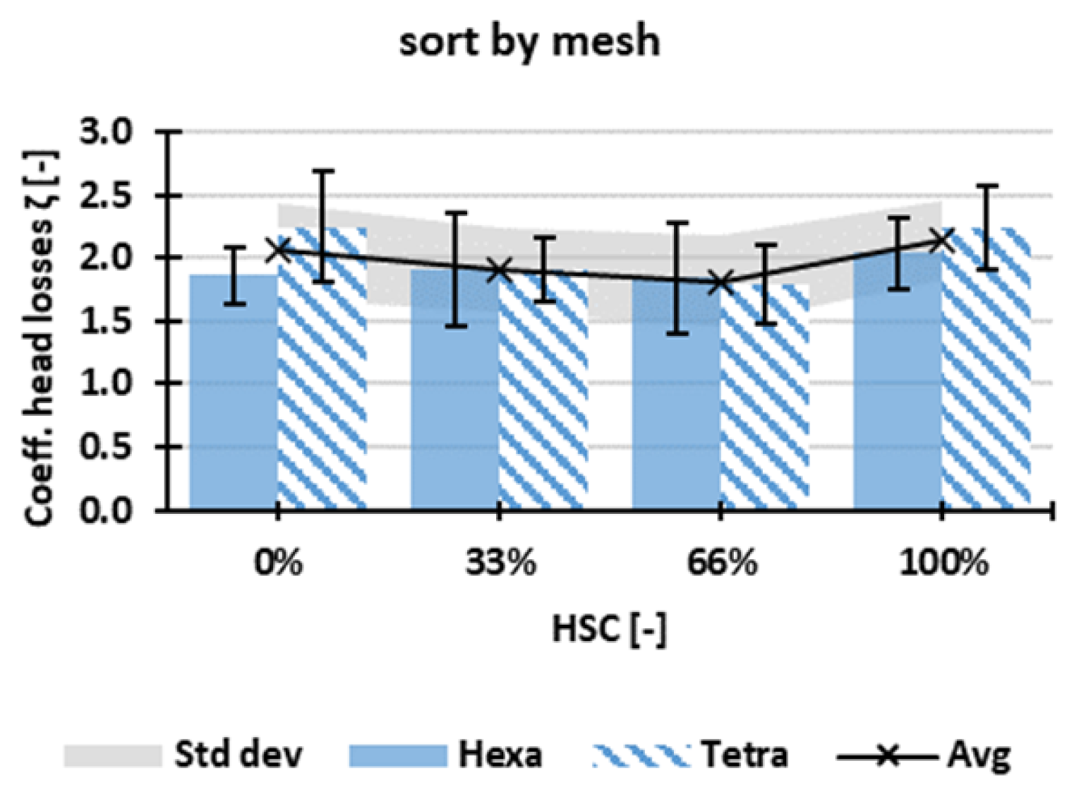
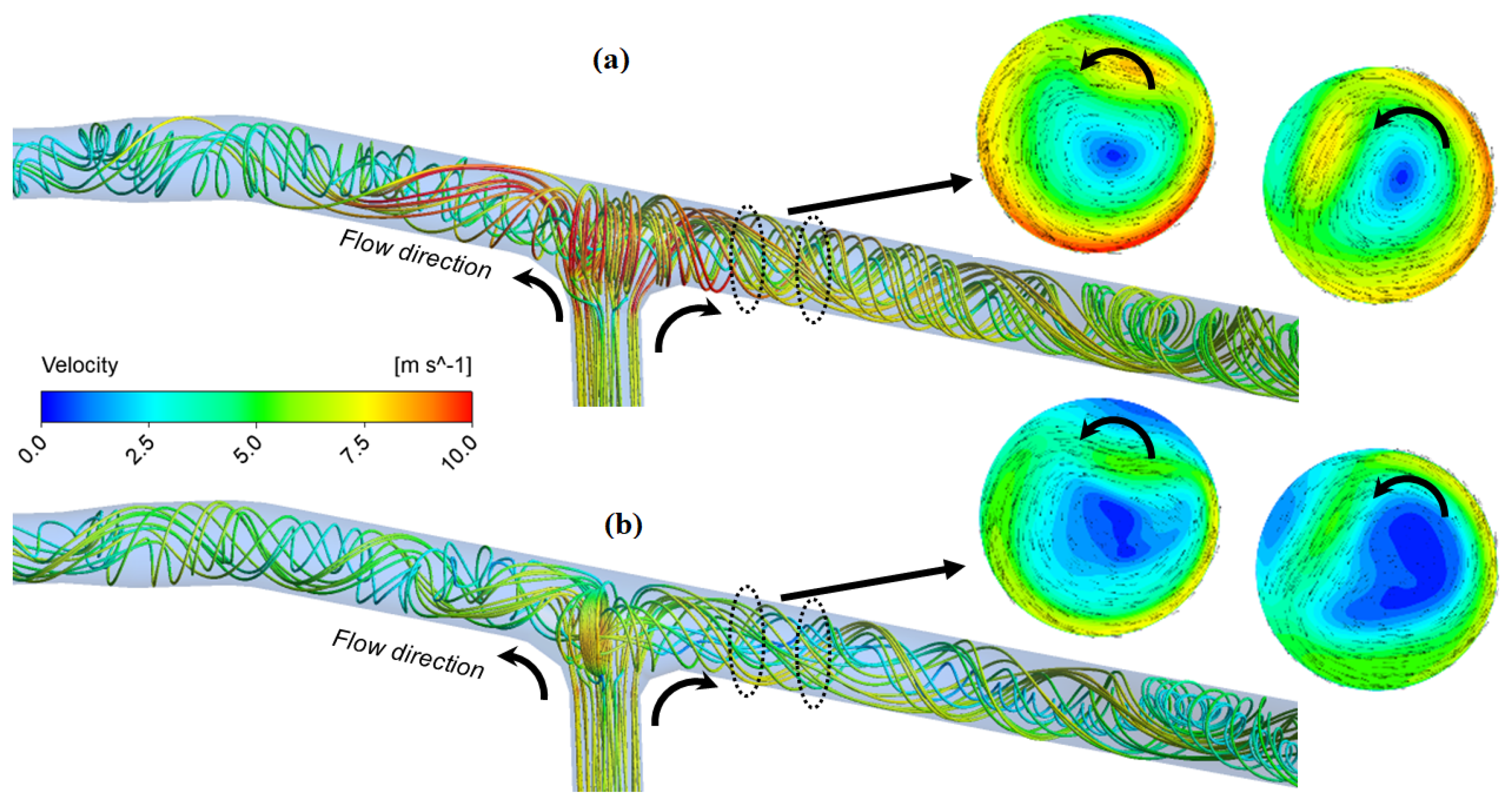
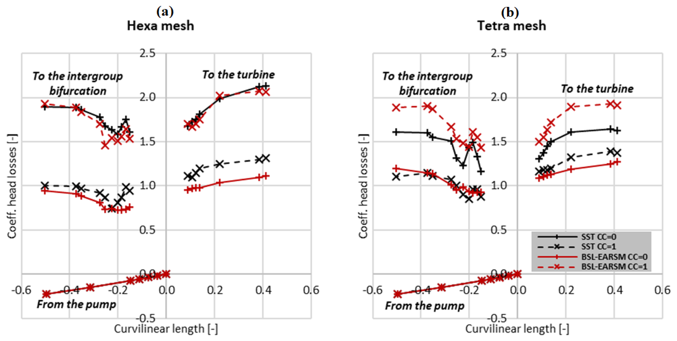
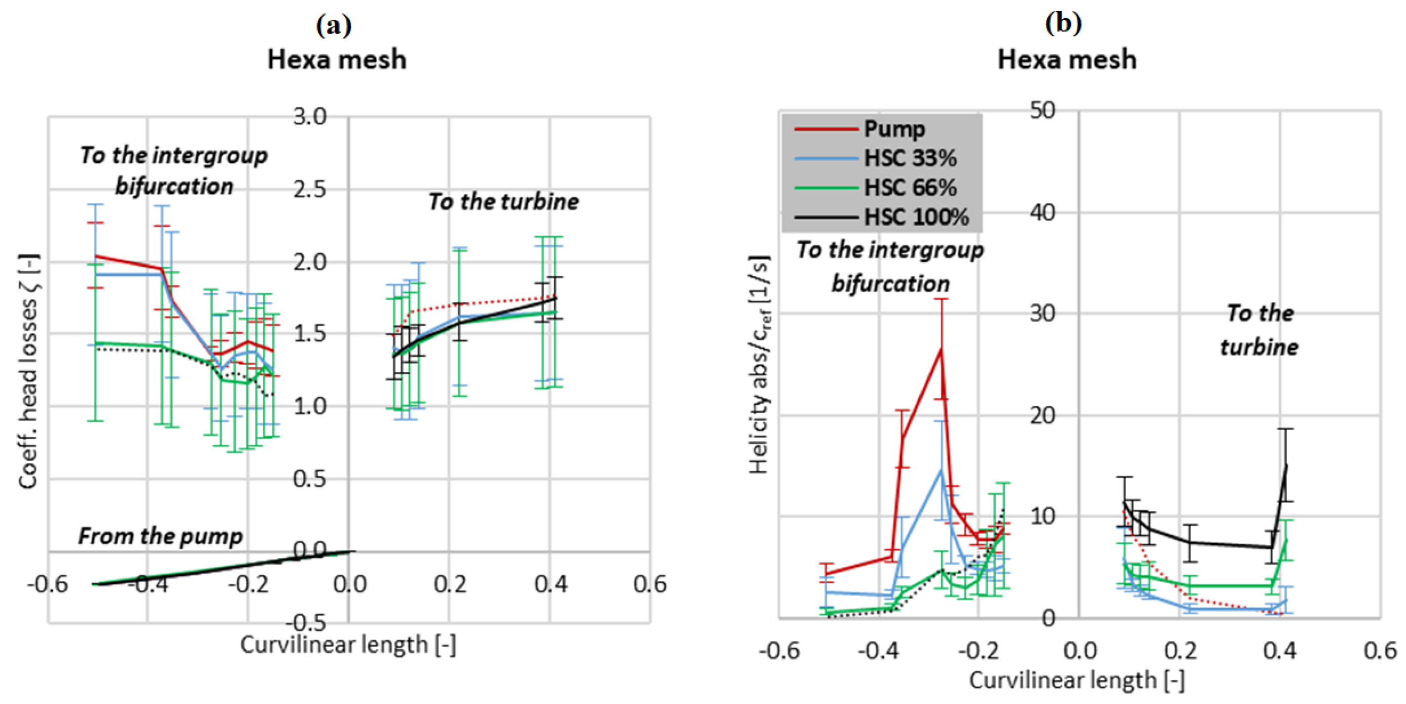
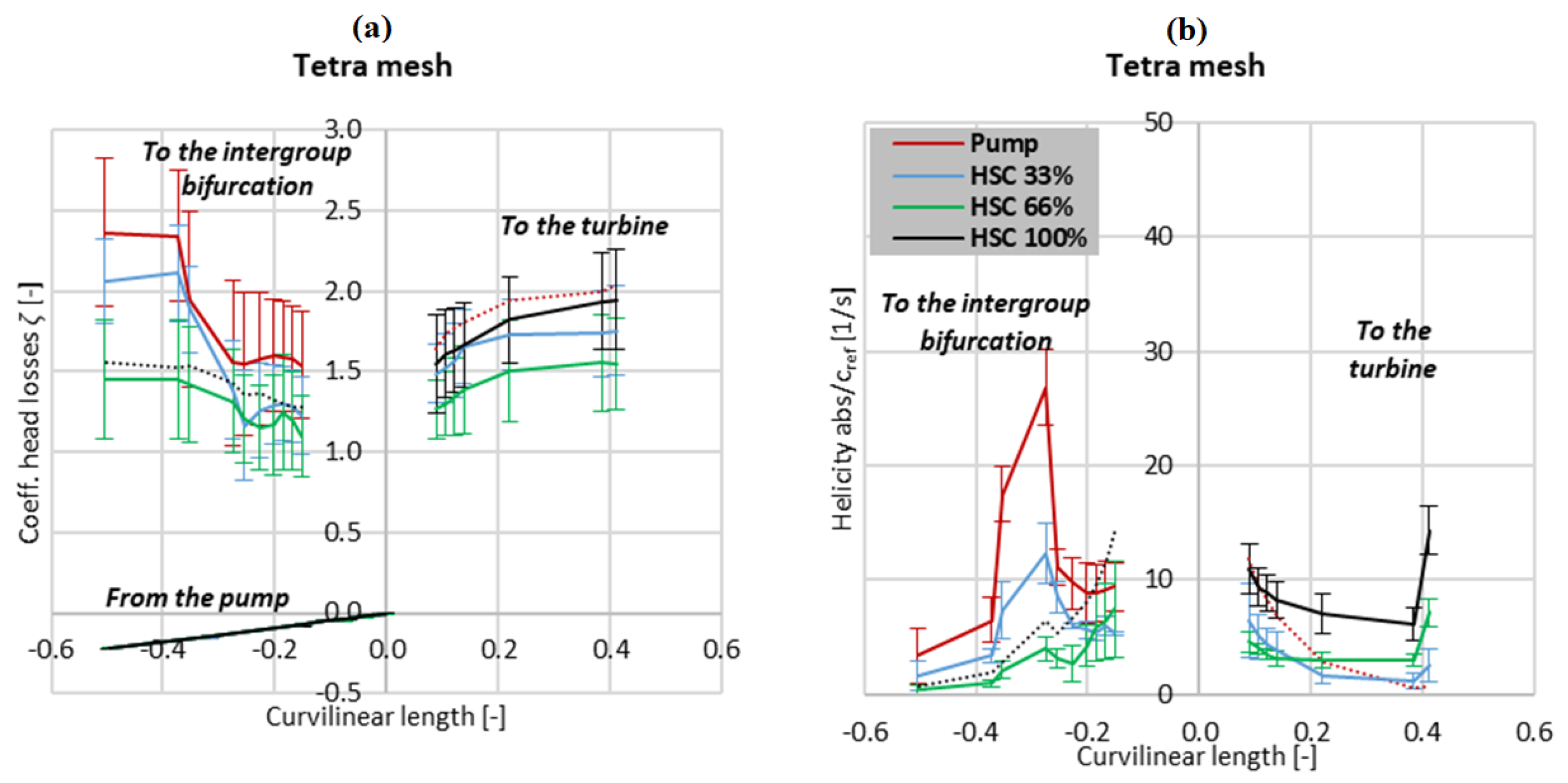
4.1. Intragroup Hsc Mode

Figure 5 compares, for the intragroup bifurcation, the head loss coefficients predicted by the simulations for each discharge ratio and each turbulence model considered. The head loss coefficient $\zeta$, defined by Equation (1), is considered between the inlet and outlet boundaries and is averaged over the last 250 iterations.

$$\zeta =\frac{p_{tot,pump}-p_{tot,turbine}}{\frac{1}{2}\rho c_{ref}^2}$$

(1)

with:

• $\rho =997$ kg/m${}^3$ the density
• $p_{tot,pump}$ the area-weighted average of the total pressure at the inlet section.
• $p_{tot,turbine}$ the area-weighted average of the average total pressure at the outlet section in the direction to the turbine
• $c_{ref}$ is the bulk flow velocity in the pumping pipe, as sketched in Figure 4.

Figure 5. Intragroup head loss coefficient in HSC mode between the pump and the turbine for 4 discharge ratio. CC = 0 stands for curvature correction switch off and CC = 1 stands for curvature correction switch on. (a) hexahedral mesh and (b) tetrahedral mesh.

Figure 5. Intragroup head loss coefficient in HSC mode between the pump and the turbine for 4 discharge ratio. CC = 0 stands for curvature correction switch off and CC = 1 stands for curvature correction switch on. (a) hexahedral mesh and (b) tetrahedral mesh.

A dispersion is noticed among the turbulence models: the standard deviation (over all the HSC operating points) reaches a value of 18.3% with the hexahedral mesh and 16.4% with the tetrahedral mesh. Regarding the influence of the curvature correction term, only the SST model shows a systematic reduction of the head loss coefficients whatever the discharge ratio by 26% for the hexahedral mesh and 19% for the tetrahedral mesh. The BSL-EARSM does not show the same tendency when the curvature correction term is activated.

To investigate the influence of the turbulence set up, the simulations are sorted either by the turbulence model used (SST or BSL EARSM) or by the activation of the curvature correction term. For each sorted category, the average and the standard deviation are computed, disregarding the influence of the other parameters. Figure 6a shows the influence of the turbulence model. The black line and the grey area correspond to the average and the standard deviation calculated over all the simulations performed. Figure 6b focuses on the influence of the curvature correction term. For most of the discharge ratios, the standard deviations (error bars) of the sorted cases span over the standard deviation computed using the full set of simulations (grey area). Consequently, it is not possible to associate some deviations to a specific set up.

Following the same way as above, in Figure 7, two sorting categories are differentiated according to the mesh (hexahedral or tetrahedral). The standard deviation amounts respectively to 18.4% and 16.4%. The chosen mesh, hexahedral or tetrahedral, remains equivalent in the uncertainty range. The 6.5% difference between hexahedral and tetrahedral mesh is contained in the uncertainty specific to the T-junction. Therefore, the main source of dispersion is not due to the mesh.

No specific trend is observed over the whole discharge ratio, except the decrease of the coefficient of head losses when the curvature correction term is activated for the SST model. Figure 8 compares the influence of the curvature correction term on the streamlines for a discharge ratio of 66%. The streamlines roll up along the pipes, due to the impinging flow on the T-junction wall. The highlighted cross sections in Figure 8 show the tangential velocity field, which put in evidence the presence of a swirling flow with a high velocity close to the pipe wall and a low velocity at the centreline. By considering the cross-section views, the tangential velocity seems lower in the case CC = 1, notably the maximal velocity magnitude decreases by 20% close to the wall. This feature could explain the lowering head losses observed in Figure 5 for the SST set-up with the CC term activated. This rotational flow could worsen the quality of the jet. This flow topology is probably not steady, this could be an explanation of the results dispersion since the simulations performed are steady simulations.

Along the pipes, the area-weighted average of the total pressure $p_{tot}$ is computed in several cross sections. The local curvilinear coordinate frame of these cross sections is defined in Figure 4. The head loss coefficient in each section is computed using Equation (2) and its evolution along the pipes is shown in Figure 9.

$$\zeta =\frac{p_{tot,ref}-p_{tot}}{\frac{1}{2}\rho c_{ref}^2}$$

(2)

The reference total pressure $p_{tot,ref}$ and bulk velocity $c_{ref}$ are considered just upstream the bifurcation, into the pump pipe (see Figure 4).

For this illustrative case of HSC 66% mode plotted in Figure 9, the main source of deviations between the turbulence models and the meshes is the singular pressure drop due to the bifurcation, virtually located at the origin of the curvilinear coordinate system. Except for this shift, the regular head losses after the bifurcation are comparable between the setups and the meshes.

Figure 10 and Figure 11 summarize, for the hexahedral and tetrahedral meshes respectively, the characteristics of the flow in the intragroup pipes for all the simulated HSC modes. On the left (Figure 10a), the average of the head loss coefficients among the four tested turbulence models is displayed along the curvilinear axis of the pipes as in Figure 9, while the error bars show the standard deviation. In Figure 10 and Figure 11, for the pumping mode and full HSC mode, the dotted line mean that no discharge flows along the concerned pipe. On the right part (Figure 10b and Figure 11b), the area-weighted average of the absolute helicity in the cross sections is shown. The helicity is defined as the volume integral of the dot product of the velocity vector with the vorticity vector [17]. It is an indicator of the number of linkages of vortex tubes in the volume and has been used for graphical visualization of vortical flows by Degani et al. [18]. In the present study the helicity is used to highlight the presence of vortices responsible for flow instabilities. The helicity is divided by a reference velocity $c_{ref}$ calculated from the average among the four turbulence models. According to the profiles of the head loss coefficients in Figure 10a, the pressure losses between the pump and the turbine occurs mainly at the bifurcation ($\zeta \approx 1.4$), independently of the flow rate ratio. In Figure 10b, the normalised helicity downstream of the T-junction is influenced by the HSC operating point. By moving from pumping mode to full HSC mode, the normalised helicity decreases in direction to the upper reservoir and increases in the direction to the turbine. This increase can be responsible for the deterioration of the quality of the jet. Despite the dispersion of the results (see the error bars), this trend is clearly visible between the HSC modes. The sharp increase in the helicity at the curvilinear positions −0.23 and 0.41 is caused by a local cross-section restriction along the pipes and an acceleration of the flow.

Concerning Figure 11, the same features as in Figure 10 are observed, except that the head loss coefficients (Figure 11a) are more dispersed downstream of the bifurcation. Despite the dispersion of the results, both meshes lead to the same conclusion. At this step, therefore, a tetrahedral mesh can be used to compute the flow in the HSC configuration.

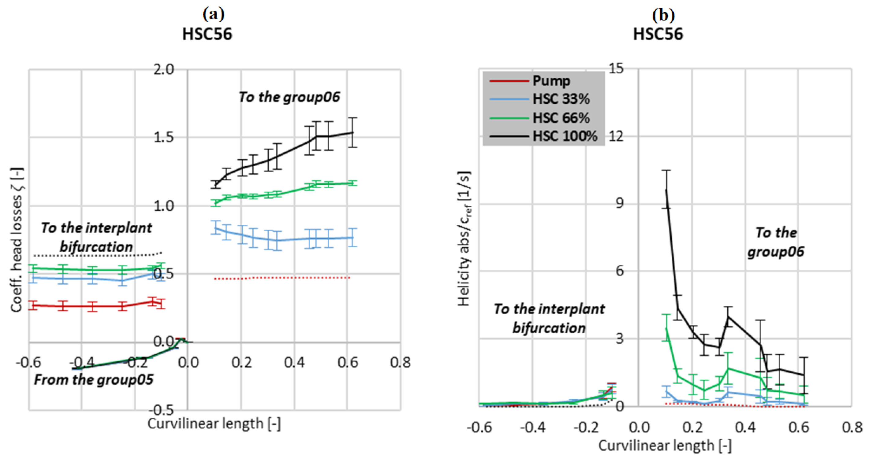
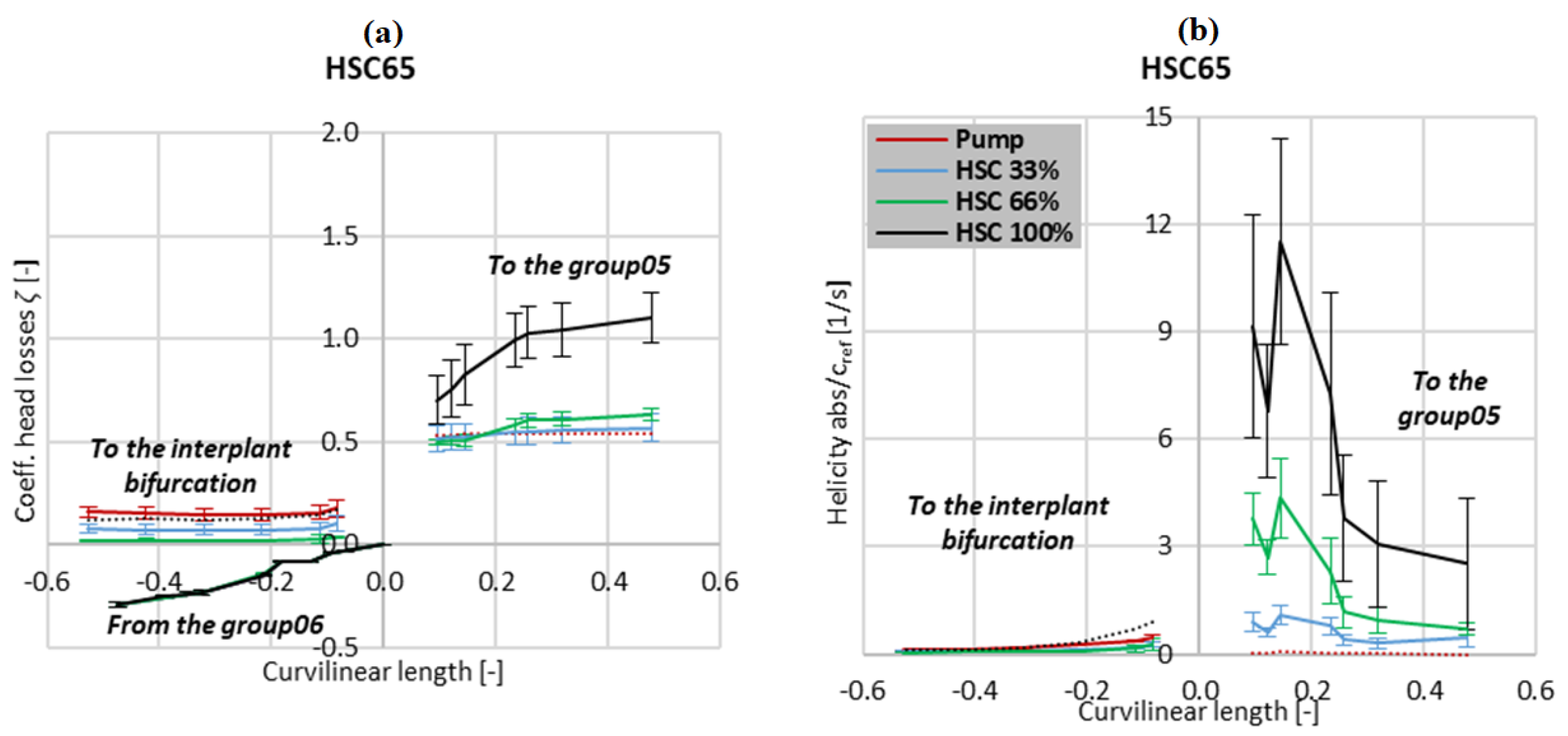
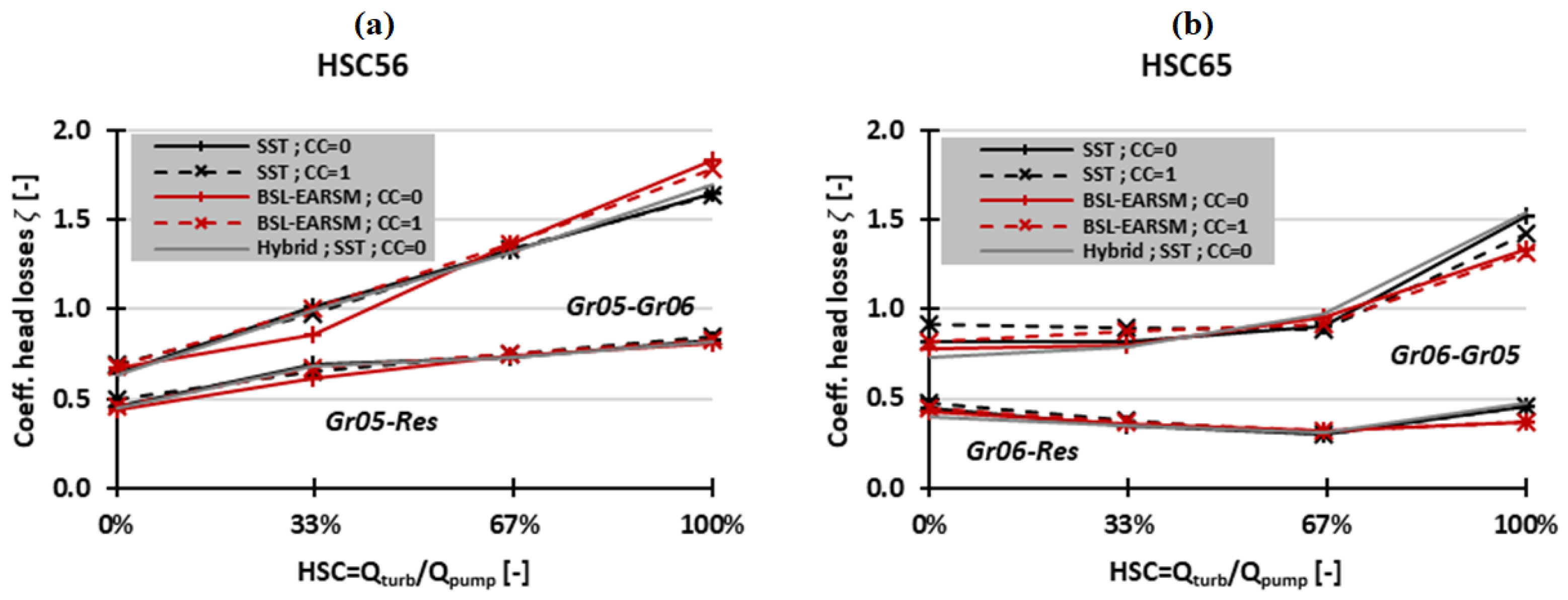
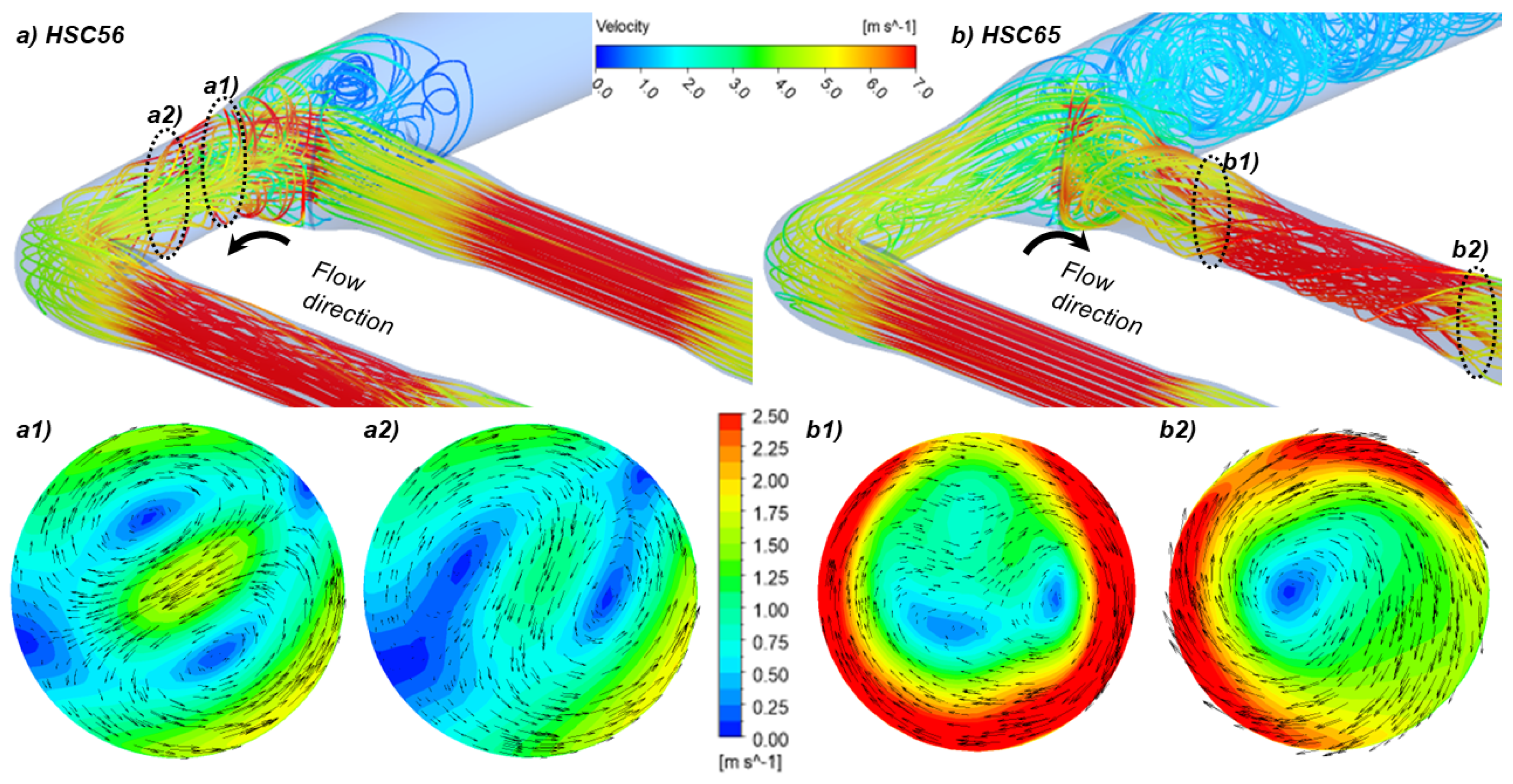
4.2. Intergroup Hsc Mode

The head loss coefficients $\zeta$ for the HSC modes at the intergroup bifurcation are reported in Figure 12, for the flow direction from group 05 to group 06 (HSC56) in Figure 12a and for the opposite direction (HSC65) in Figure 12b. Among the different set-ups, the dispersion is lower than the one observed for the previous intragroup bifurcation, with a standard deviation of 3.5% for HSC56 and 6.5% for HSC65. The results of the hybrid mesh remain in the standard deviation range. The hybrid mesh is thus considered as equivalent to the tetrahedral mesh.

Figure 13 and Figure 14 show the profiles of the head loss coefficients and of the helicity for case HSC56 and case HSC65 respectively (the hybrid mesh is excluded from the averaged curves). It is noticed that the head loss coefficient between the pump and the turbine increases with the percentage of HSC and the losses are mainly concentrated at the junction ($\zeta$ between 0.50 and 1.23). For the HSC65 case (Figure 14), the head loss coefficient increases suddenly for an HSC at 100% compared to the case HSC56 (Figure 13), for which the head loss coefficient increases more regularly. The largest head loss coefficients in the HSC56 case are explained by the flow impinging the wall at the bifurcation (see Figure 15a), contrary to the HSC65 (Figure 15b). The normalised helicity, in Figure 13b and Figure 14b, increases with the percentage of HSC. Due to the highest discharge into the turbine branch and the highest intensity of the secondary flow, HSC 100% case is the most critical operating point. The helicity jump on the turbine side is caused by a cross-section restriction along the pipes and an acceleration of the flow.

The flow topology is illustrated in Figure 15, with the streamlines rolling up downstream the junction. As displayed in Figure 15(a1–b2), the tangential velocity vectors have not the same structure downstream of the bifurcation depending on the flow direction. The velocity near the wall seems larger for HSC from group 6 to 5 (Figure 15(b1,b2). In Figure 15(a1), a Dean vortex [19] appears downstream of the bifurcation in HSC56 mode.

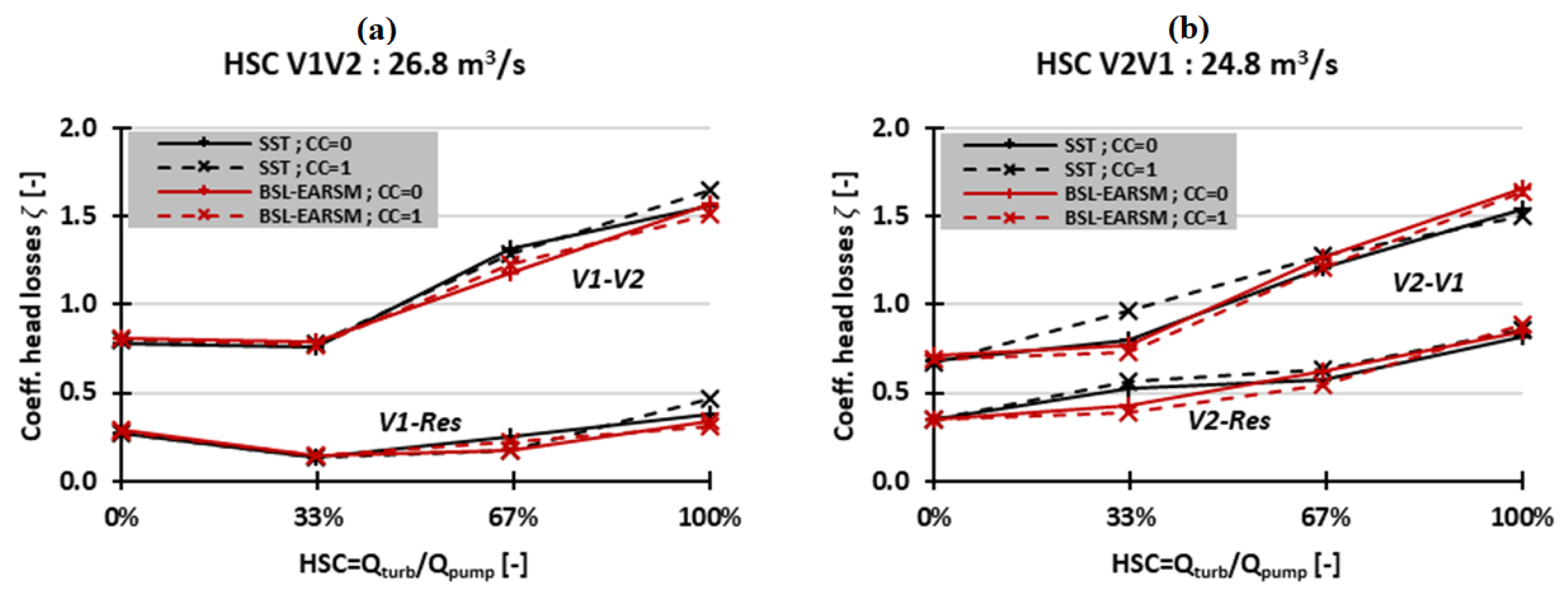
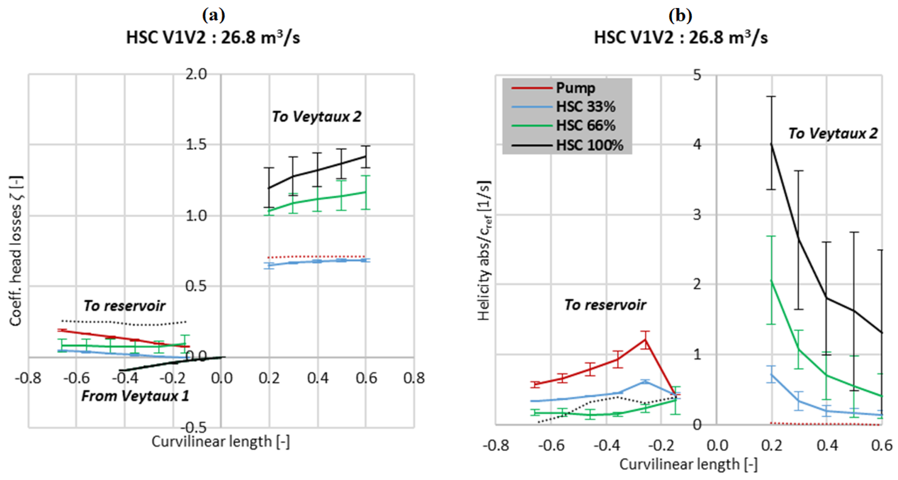
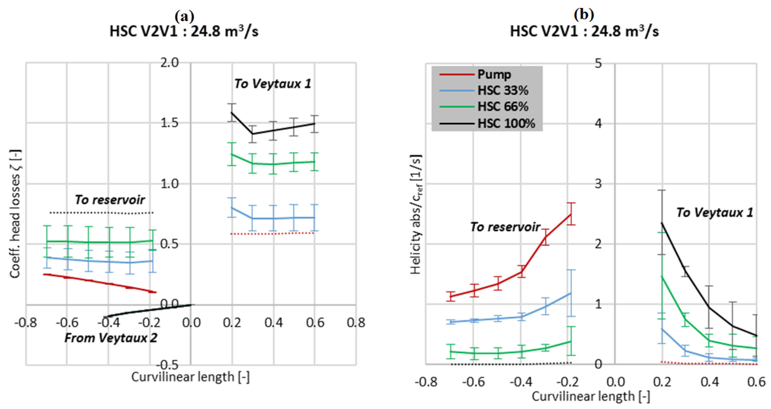
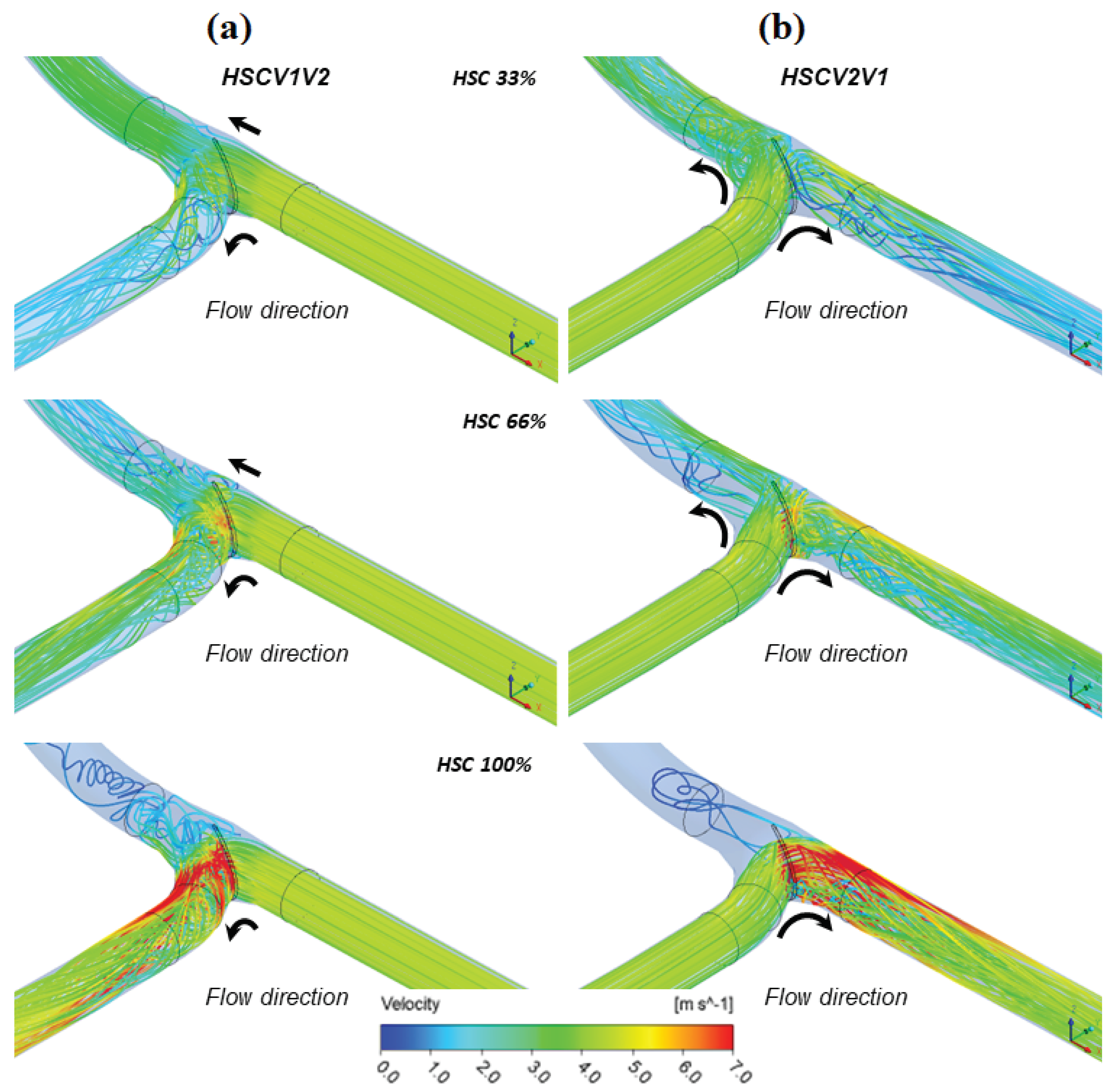
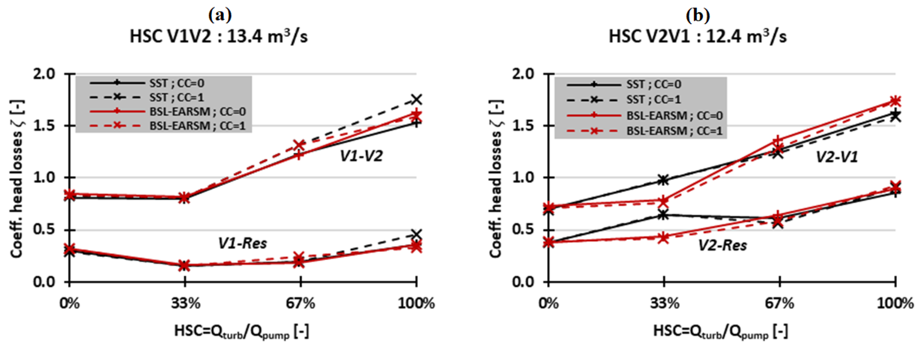
4.3. Interplant Hsc Mode

The head loss coefficients $\zeta$ predicted by each turbulence model are plotted in Figure 16 for the interplant bifurcation, with in Figure 16a the HSC mode with pumping from Veytaux 1 to Veytaux 2 (HSC V1V2) and in Figure 16b the HSC mode with pumping from Veytaux 2 to Veytaux 1 (HSC V2V1). These results represent the operation of the HSC mode with the maximum possible flow rate, i.e., all the pumps of the powerhouse are running, which corresponds to a discharge of 26.8 m³/s and 24.8 m³/s for the HSC V1V2 and HSC V2V1 modes respectively (see Table 2). As for the intergroup bifurcation, the dispersion between the models is rather low (6.9% of standard deviation reported for the case HSC V1V2 and 6.6% for the case HSC V2V1), even by using a hybrid mesh.

The same head loss coefficients are illustrated in Figure 17 but for a pumped flow rate divided by two with a value of 13.4 m³/s and 12.4 m³/s respectively (see Table 2). The magnitude of the head loss coefficients remains similar. The direction of the flow in HSC mode (V1 to V2 or V2 to V1) does not seem to significantly influence the head loss coefficients, except for the coefficient between the pump and the reservoir. But this last one is not considered as critical in the framework of this study.

Figure 18 (V1V2) and Figure 19 (V2V1) show the head loss coefficient (Figure 18a and Figure 19a) and the normalised absolute helicity (Figure 18b and Figure 19b) profiles for the maximum flow rate. The pressure losses between the pump and the turbine are mainly concentrated at the bifurcation. By deviating more flow to the turbine, the head loss coefficient and the normalised helicity in the direction of the turbine increase. The helicity in HSC V2V1 mode (Figure 19b) appears to generate less helicity in turbine branch than in the HSC V1V2 mode (Figure 18b) by an order of magnitude of 2. The head loss coefficient in the configuration HSC V2V1 (Figure 19a) seems to flatten in the turbine pipe, which correspond to a diminution of the linear head losses. The absence of the pipe bend after the bifurcation (compared to the reverse direction HSC V1V2) is probably the explanation.

The streamlines coloured by the velocity are shown in Figure 20, where it is noticeable that by increasing the flow rate ratio, the velocity at the bifurcation increases. This is an explanation for the increase in the head losses between the pump and the turbine by increasing the flow rate.

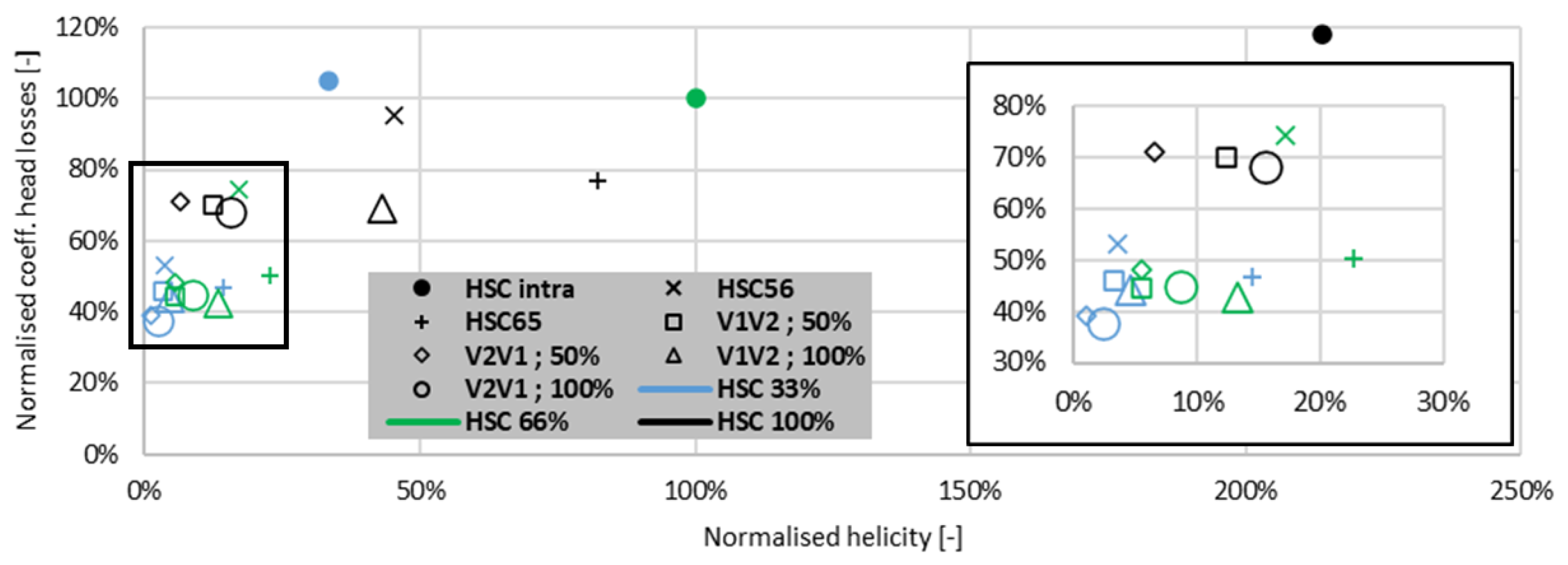
5. Comparison of the Bifurcations

Table 3. Head loss coefficient between the pump and the turbine. Comparison between the different bifurcations in function of HSC.

	Intragroup	Intergroup 56	Intergroup 65	Interplant Single Flowrate V1V2	Interplant Single Flowrate V2V1	Interplant Double Flowrate V1V2	Interplant Double Flowrate V2V1
HSC 33%	105%	53%	47%	46%	39%	44%	38%
HSC 66%	100%	74%	50%	45%	48%	43%	45%
HSC 100%	118%	95%	77%	70%	71%	69%	68%

and

Table 4. Normalised helicity into the turbine pipe. Comparison between the different bifurcations in function of HSC.

	Intragroup	Intergroup 56	Intergroup 65	Interplant Single Flowrate V1V2	Interplant Single Flowrate V2V1	Interplant Double Flowrate V1V2	Interplant Double Flowrate V2V1
HSC 33%	33%	4%	14%	3%	1%	5%	2%
HSC 66%	100%	17%	23%	6%	5%	13%	9%
HSC 100%	214%	45%	82%	12%	7%	43%	16%

summarise the head loss coefficients $\zeta$ between the pump and the turbine as well as the helicity in the turbine pipe for the three bifurcations and the different HSC configurations studied. All the results are compared with the intragroup HSC mode at 66%, which is currently the highest percentage of HSC mode permitted. The head loss coefficients for the intergroup and interplant HSC modes are lower than for the intragroup HSC, even if for the intergroup HSC56 at 100% the coefficient reaches 95%. According to Table 4, all the intergroup and interplant HSC modes generate less helicity than the intragroup HSC.

The normalised head loss coefficient is plotted against the normalised helicity in Figure 21. For the intragroup bifurcation, which is a T-junction, whatever the discharge ratio the head loss coefficient is almost constant and insensitive to the helicity magnitude. For the two other bifurcations, the head loss coefficient increases with the helicity and the discharge ratio. Therefore, the geometry of the bifurcation influences the magnitude of the head loss coefficient and the helicity. Best performances are expected in terms of head losses and flow disturbance by operating the HSC interplant configuration, for which the head losses should represent less than 10% of the head losses in the whole piping system.

Regarding the flow topology, some conclusions can be drawn by comparing the velocity vectors and contours plotted in a mid-plane of the bifurcations (see Figure 22). For the intragroup T-bifurcation, the flow from the pump impinges the opposite wall leading to the development of recirculation zones downstream. The magnitude of the velocity reaches values larger than 10 m/s. On the contrary, for the other bifurcations, only one recirculation zone just downstream the bifurcation is observed. The magnitude of the velocity is lower reaching values around 6 m/s for the intergroup bifurcation and less than 4 m/s for the interplant bifurcation. For these two last bifurcations, the flow looks like the one in a strongly curve pipe, whereas for the T-junction the flow looks like a jet impinging a flat plate. This impingement seems to be responsible for the high head losses and helicity level.

Based on these results and compared to the current HSC configuration permitted, both the intergroup and the interplant HSC configurations could be operated without risk, which would improve the flexibility of the power plant operation. In addition, a T-junction should be avoid for operating in HSC mode since this geometry promotes the increase in both head losses and helicity.

6. Conclusions

This paper assesses the possibility of extending the HSC mode at the FMHL/FMHL+ powerplant by performing steady CFD simulations of three existing bifurcations.

The influence of the mesh and the turbulence model (SST $k-\omega$ and BSL-EARSM) including the effect of the CC term is investigated. The head loss coefficients for the intragroup bifurcation, which is a T-junction, show a strong dependence on the mesh and the turbulence model (standard deviation of 17.4%) contrary to the two Y-junctions. With the SST $k-\omega$, the activation of the CC generates a decrease by 23% of the head loss coefficients. This discrepancy among the intragroup results can be explained by the T-junction geometry since the topology of the flow looks like a jet impinging a wall that then splits in two swirling flows.

The intergroup and interplant HSC configurations achieve better performances compared to the intragroup HSC mode with lower head losses and a lower magnitude of the helicity, even for a discharge ratio of 100%; the HSC mode from Veytaux 2 to Veytaux 1 being the best configuration.

Several future investigations can be considered: to validate the head losses computed by performing on-site measurements, to simulate the flow until the Pelton turbine to check if the quality of the jet is not altered in HSC mode compared to the turbine mode, to performed unsteady simulations mainly for the T-junction to investigate if the discrepancy between the results can be reduced and to perform velocity measurements on a reduced scale model to better understand the flow topology and to improve the validation of the CFD results.

References

1. Guittet, M.; Capezzali, M.; Gaudard, L.; Romerio, F.; Vuille, F.; Avellan, F. Study of the drivers and asset management of pumped-storage power plants historical and geographical perspective. Energy 2016, 111, 560–579. [Google Scholar] [CrossRef]
2. Rocks, A.; Meusburger, P. The Electrical Asset and Mechanical Machinery of Obervermuntwerk II. Wasserwirtsch 2015, 105, 48–52. [Google Scholar] [CrossRef]
3. Micoulet, G.; Jaccard, A.; Rouge, N. FMHL+: Power extension of the existing Hongrin-Léman powerplant: From the first idea to the first kWh. In Proceedings of the Hydro Conference, Montreux, Switzerland, 10–12 October 2016. [Google Scholar]
4. Pérez-Díaz, J.I.; Sarasúa, J.I.; Wilhelmi, J.R. Contribution of a hydraulic short-circuit pumped-storage power plant to the load–frequency regulation of an isolated power system. Int. J. Electr. Power Energy Syst. 2014, 62, 199–211. [Google Scholar] [CrossRef]
5. Decaix, J.; Biner, D.; Drommi, J.-L.; Avellan, F.; Münch-Alligné, C. CFD simulations of a Y-junction for the implementation of hydraulic short-circuit operating mode. IOP Conf. Ser. Earth Environ. Sci. 2021, 774, 012013. [Google Scholar] [CrossRef]
6. Huber, B.; Korger, H.; Fuchs, K. Hydraulic Optimization of a T-junction–Hydraulic Model Tests and CFD Simulation. In Proceedings of the XXXI IAHR Congress, Seoul, Republic of Korea, 11–16 September 2005. [Google Scholar]
7. Decaix, J.; Drommi, J.-L.; Avellan, F.; Münch-Alligné, C. CFD simulations of hydraulic short-circuits in junctions, application to the Grand’Maison power plant. IOP Conf. Ser. Earth Environ. Sci. 2022, 1079, 012106. [Google Scholar]
8. HydroLEAP–Modernizing the Swiss Hydropower Fleet for a Successful Energy Strategy 2050; Annual Report. Available online: https://www.aramis.admin.ch/Dokument.aspx?DocumentID=69905 (accessed on 17 May 2022).
9. Schlipf, M.; Tismer, A.; Riedelbauch, A. On the application of hybrid meshes in hydraulic machinery CFD simulations. IOP Conf. Ser. Earth Environ. Sci. 2016, 49, 2013. [Google Scholar] [CrossRef]
10. Kwak, D.; Kiris, C.C. Computation of Viscous Incompressible Flows; Springer GmbH: Berlin/Heidelberg, Germany, 2010. [Google Scholar]
11. Menter, F.R. Review of the shear-stress transport turbulence model experience from an industrial perspective. IOP Int. J. Comput. Fluid Dyn. 2009, 23, 305–316. [Google Scholar] [CrossRef]
12. Wallin, S.; Johansson, A.V. An explicit algebraic Reynolds stress model for incompressible and compressible turbulent flows. J. Fluid Mech. 2000, 403, 89–132. [Google Scholar] [CrossRef]
13. Smirnov, P.E.; Menter, F.R. Sensitization of the SST Turbulence Model to Rotation and Curvature by Applying the Spalart–Shur Correction Term. J. Turbomach. 2002, 131, 89–132. [Google Scholar] [CrossRef]
14. Wallin, S.; Johansson, A.V. Modelling streamline curvature effects in explicit algebraic Reynolds stress turbulence models. Int. J. Heat Fluid Flow 2002, 23, 721–730. [Google Scholar] [CrossRef]
15. Menter, F.R.; Ferreira, J.; Esch, T.; Konno, B. The SST Turbulence Model with Improved Wall Treatment for Heat Transfer Predictions in Gas Turbines. In Proceedings of the International Gas Turbine Congress, Tokyo, Japan, 2–7 November 2003. [Google Scholar]
16. Durbin, P.; Pettersson-Reif, B.A. Statistical Theory and Modeling for Turbulent Flows; Wiley: Hoboken, NJ, USA, 2011; Volume 376. [Google Scholar]
17. Bailly, C.; Comte-Bellot, G. Turbulence; Springer GmbH: Berlin/Heidelberg, Germany, 2015. [Google Scholar]
18. Degani, D.; Seginer, A.; Levy, Y. Graphical visualization of vortical flows by means of helicity. AIAA J. 1990, 28, 1347–1352. [Google Scholar]
19. Kalpakli Vester, A.; Örlü, R.; Alfredsson, P.H. Turbulent Flows in Curved Pipes: Recent Advances in Experiments and Simulations. Appl. Mech. Rev. 2016, 68, 721–730. [Google Scholar] [CrossRef]
Figure 1. 3D view of the pipes of the FMHL+ powerplant with the different possibilities of HSC modes. The red arrow refers to the intra-group HSC mode, the green arrow to the intergroup HSC mode and the blue arrow to the inter-plant HSC mode.
Energies 17 00473 g001
Figure 2. Fluid domain for: (a) the intragroup HSC mode, (b) the intergroup HSC mode and (c) the interplant HSC mode. Black arrows indicate the location to which the pipe is connected. Red arrows highlight the location of the reinforcement at the bifurcations.
Energies 17 00473 g002
Figure 3. View of the meshes of the intragroup, intergroup and the interplant bifurcations.
Energies 17 00473 g003
Figure 6. (a), Average (column) and standard deviation (error bar) of the head loss coefficient depending on the turbulence model considered (SST or BSL EARSM). (b), Average (column) and standard deviation (error bar) of the head loss coefficient depending on the activation of the curvature correction term. The black line with the cross and the grey area refer to the average and the standard deviation of the head loss coefficient calculated over the full set of simulations respectively.
Energies 17 00473 g006
Figure 7. Average and standard deviation of coefficient of head losses on the T-bifurcation. Differentiation between the meshes.
Energies 17 00473 g007
Figure 8. Streamlines coloured by the velocity with a highlight on the tangential velocity vectors in two cross sections in the direction of the turbine. (a) CC = 0 and (b) CC = 1. Discharge ratio of 66%. SST k- ω model. Hexahedral mesh.
Energies 17 00473 g008
Figure 9. Head loss coefficient profile along the three pipes of intragroup bifurcation at HSC 66% mode among the various turbulence model and curvature correction. (a) hexahedral mesh and (b) tetrahedral mesh.
Energies 17 00473 g009
Figure 10. (a) head loss coefficient profile along the three pipes of intragroup bifurcation at different HSC modes. (b) normalised absolute helicity profile. Hexahedral mesh.
Energies 17 00473 g010
Figure 11. (a) head loss coefficient profile along the three pipes of intragroup bifurcation at different HSC modes. (b) normalised absolute helicity profile. Tetrahedral mesh.
Energies 17 00473 g011
Figure 12. Intergroup head loss coefficient between the pump and the turbine and between the pump and the reservoir at different HSC operating modes for the considered turbulence models. (a) HSC mode from group red5 to group red6. (b) HSC from group red6 to group red5. Tetrahedral and hybrid meshes.
Energies 17 00473 g012
Figure 13. (a) head loss coefficient profile along the three pipes of intergroup bifurcation at different HSC mode from group 5 to group 6. (b) normalised absolute helicity profile. Tetrahedral mesh.
Energies 17 00473 g013
Figure 14. (a) head loss profile along the three pipes of intergroup bifurcation at different HSC modes from group 6 to group 5. (b) absolute helicity profile. Tetrahedral mesh.
Energies 17 00473 g014
Figure 15. Streamlines coloured by velocity in the intragroup bifurcation for 100% HSC. Highlight on tangential velocity vectors in cross-section toward the turbine direction. SST model CC = 0 and Tetrahedral mesh. (a) HSC56 and (b) HSC65.
Energies 17 00473 g015
Figure 16. Interplant head loss coefficient between the pump and the turbine and between the pump and the reservoir for different HSC operating modes and tested turbulence models. (a) HSC with pumping from Veytaux I to Veytaux II. (b) HSC with pumping from Veytaux II to Veytaux I. Double flow rate is considered: 26.8 m3/s and 24.8 m3/s respectively.
Energies 17 00473 g016
Figure 17. Interplant head loss coefficient between the pump and the turbine and between the pump and the reservoir for different HSC operating modes and for the tested turbulence models. (a) HSC with pumping from Veytaux I to Veytaux II. (b) HSC with pumping from Veytaux II to Veytaux I. Single flowrate is considered: 13.4 m3/s and 12.4 m3/s respectively.
Energies 17 00473 g017
Figure 18. (a) the head loss coefficient profiles along the three pipes of interplant bifurcation at different HSC modes between Veytaux I and Veytaux II for a double flow rate. (b) normalised absolute helicity profiles.
Energies 17 00473 g018
Figure 19. (a) the head loss coefficient profiles along the three pipes of interplant bifurcation at different HSC modes between Veytaux II and Veytaux I for a double flow rate. (b) normalised absolute helicity profiles.
Energies 17 00473 g019
Figure 20. Streamlines coloured by velocity in the interplant bifurcation for 33–66–100% HSC. SST model CC = 0. (a) HSC pumped from Veytaux I and turbined in Veytaux II. (b) HSC pumped from Veytaux II and turbined in Veytaux I. Double flowrate considered resp. 26.8 m3/s and 24.8 m3/s.
Energies 17 00473 g020
Figure 21. Normalised helicity according to the normalised helicity for all simulated scenarios with a highlight on the close area framed in black.
Energies 17 00473 g021
Figure 22. Velocity contours and vectors plotted in a mid-plane of each bifurcation. (a) intragroup HSC mode in the T-junction; (b) intergroup HSC mode between group 5 and 6; (c) intergroup HSC mode between group 6 and 5; (d) interplant HSC mode between Veytaux 1 et Veytaux 2 and (e) interplant HSC mode between Veytaux 2 et Veytaux 1. Pumping discharge set to 12.4 m3/s and HSC mode for a discharge ratio of 100%. Simulation with the SST model without curvature correction.
Energies 17 00473 g022