Optimal Power Flow Management for a Solar PV-Powered Soldier-Level Pico-Grid

Abstract

Users ought to decide how to operate and manage power systems in order to achieve various goals. As a result, many strategies have been developed to aid in this regard. Optimal power flow management is one such strategy that assists users in properly operating and managing the supply and demand of power in an optimal way under specified constraints. However, in-depth research on optimal power flow management is yet to be explored when it comes to the supply and demand of power for the bulk of standalone renewable energy systems such as solar photovoltaics, especially when it comes to specific applications such as powering military soldier-level portable electronic devices. This paper presents an optimal power flow management modelling and optimisation approach for solar-powered soldier-level portable electronic devices. The OPTI toolbox in MATLAB is used to solve the formulated nonlinear optimal power flow management problem using SCIP as the solver. A globally optimal solution was arrived at in a case study in which the objective function was to minimise the difference between the power supplied to the portable electronic device electronics and the respective portable electronic device power demands. This ensured that the demand for solar-powered soldier-level portable electronic devices is met at all times in spite of the prohibitive case scenarios’ circumstances under the given constraints. This resolute approach underscores the importance placed on satisfying the demand needs of the specific devices while navigating and addressing the limitations posed by the existing conditions or constraints. Soldiers and the solar photovoltaic user fraternity at large will benefit from this work as they will be guided on how to optimally manage their power systems’ supply and demand scenarios. The model developed herein is applicable to any demand profile and any number of portable electronic device and is adaptable to any geographical location receiving any amount of solar radiation.

1. Introduction

The largest and most intricate human-made system in the world, the U.S. electric network, is extremely susceptible to three different sorts of outside vulnerabilities: natural catastrophes, deliberate physical attacks, and cyberattacks [1]. Employing renewable energy technologies (RETs) which encompass distributed generation and microgrids, such as those of solar photovoltaic (PV) systems, to safeguard the grid and render it more resistant to attacks is gaining mileage in recent times. However, in-depth research and development are yet to be explored when it comes to optimal power management of such RETs, especially when it comes to soldier-level military applications.

The soldier is at risk when carrying bulky amounts of non-rechargeable batteries. Thus, the need for shifting to RETs such as solar PV which allow for portable power generation, supply, and consumption is of paramount importance. Solar-PV blankets, vests, helmets, and backpacks which can recharge batteries in portable electronic devices (PEDs) are among the renewable energy technologies used by the U.S. military [2]. This enables soldiers to power their individual and troop PEDs while on combat missions. Many developing and developed countries, inclusive of the U.S., are accelerating the deployment of solar energy in their military applications [3,4]. Nonetheless, much still needs to be done when it comes to soldier-level power generation, consumption, and the respective optimal power management both from the supply and demand sides. Portable, robust, and dependable power is needed for the PEDs and accessories used by soldiers to communicate and carry out their missions in an intelligent and effective manner. To enable the soldiers to carry out their missions and securely traverse foreign environments, the power consumption of soldier-level military-grade PEDs should be ascertained and optimally managed.

Modern energy and power systems have substantially expanded and are still growing, owing to the advancement and development of technology [5]. In order to properly manage these increasingly intricate energy systems, technologically advanced computer approaches are demanded. Modelling and optimisation of these complex energy and power systems incorporating mathematical and analytical tools with the likes of MATLAB is one such approach. The proposed modelling and optimisation approach in this study uses the OPTI Toolbox, a robust optimisation toolbox integrated into MATLAB, which when combined with the SCIP (Solving Constraint Integer Programs) solver, presents a formidable system for addressing intricate optimisation problems. SCIP is a framework for solving mixed-integer nonlinear systems, which are a subset of constraint integer programming (CIPs). It works as both an architecture for mixed-integer programming (MIP) and mixed-integer nonlinear programming (MINLP) [6,7].

Optimal power management can be applied to various domains, such as buildings, vehicles, aircraft, marine vessels, renewable energy power supply systems, hybrid energy systems, and electric grids among others. Optimal power management is the process of using power in the most efficient way possible, by sensing when and where power is needed most and distributing it dynamically among different PEDs or systems [8]. Optimal power flow management problems are an indispensable issue in the planning and execution of modern power systems. The aim of optimum power flow management is to find the best optimal approach and decision parameters for minimizing losses, reducing emissions, lowering costs, meeting demand, managing supply, or amalgamating the aforementioned goals. It often involves using optimisation techniques or algorithms to find the best way to manage the power sources, loads, and storage PED in a given system or scenario [9].

Some examples of optimisation methods are dynamic programming, reinforcement learning, artificial neural networks, fuzzy logic, and so on [10]. The optimisation methods can incorporate linear, nonlinear, quadratic, mixed integer, and/or binary approaches depending on the nature of problem formulation and desired outcomes. These methods can also help to find the optimal trade-off between different objectives, such as fuel consumption, emissions, performance, cost, and so on [11]. Optimal power management can help save energy and money by avoiding the wasteful or unnecessary use of power, such as when PEDs are idle or not in use [12]. It can help enhance the performance and reliability of PEDs or systems by ensuring that they have enough power to operate properly and avoid overheating or damage. Sustainability and environmental benefits can be increased through optimal power management by reducing greenhouse gas emissions and pollution by promoting the use of renewable energy sources or minimizing the use of fossil fuels. This current research adopts a nonlinear programming method in conjunction with mathematical analytical tools to ascertain optimal power management for solar PV-powered soldier-level PEDs.

When it comes to the optimisation of the different energy systems, many previous works tackle the supply side of things, having the objective of minimising fuel consumption, in the case of hybrid systems ensuring that priority is given to RETs rather than conventional sources [13,14,15,16,17]. Some existing optimisations target the reduction of pollutant emissions such as carbon monoxide, carbon dioxide, and sulphur oxides among other hazardous gasses in a bid to combat climate change [18,19,20]. Other reported works focus on minimising drawing power from the grid and maximising the use of RETs and storage batteries [21,22,23,24,25]. Optimisations that tackle multi-objectives targeting the technical, economic, and environmental aspects among others have also been reported on [26,27,28,29,30,31,32]. To the best knowledge of the authors, no previous research was found to have reported on power/energy optimisation of solar PV-powered soldier-level military PED. The proposed modelling and optimisation method addresses the aforementioned problems and attempts to give the best approach to optimally manage the power flows of solar PV-powered soldier-level military PED.

Section 2 gives the problem formulation and the respective modelling and optimisation entailed. Section 3 gives the modelling and optimisation, Section 4 gives the case study, Section 5 gives the results, and discussion and Section 6 concludes the paper.

2. Problem Formulation

Figure 1 illustrates the proposed system to be modelled and optimised. Part of the figure (depicted by the red circle) is extrapolated to show how power flows in the laptop (one of the PEDs) which is typical for all the PEDs. In the extrapolation, $B_{LAP}$ refers to the laptop battery and $E_{LAP}$ refers to the laptop electronics. The modelling and optimisation approach taken in this research is not constrained to specific PEDs and is not confined to a certain number of the same. Each PED has its own specific PED electronics demand and an embedded battery of a certain capacity. The solar panel is integrated into the backpack and additional foldable solar blankets can also be used as standalone or as additional solar collectors for incoming solar radiation. The main battery can be integrated within the solar backpack or can be a separate one to be packaged into the backpack.

Figure 2 shows the modelling approach taken and how power flows within the proposed system. The main battery receives power from the solar PV system, and the PED batteries receive power from solar PV and also from the main battery. The respective PED electronics power demands are supplied by the respective PED batteries and also directly from the main battery and solar PV.

3. Modelling and Optimisation

Modelling and optimisation of energy systems are crucial steps in designing efficient and cost-effective renewable energy solutions [33,34]. In the case of solar PV, in this process, mathematical models are developed to simulate the behaviour of the systems, taking into account factors such as panel efficiency, solar irradiance, and shading effects, among others. These models enable the prediction of power output, performance, and energy production of the system under different conditions. Modelling and optimisation contribute immensely to the successful implementation of solar PV systems and the overall energy management of the same. By using optimisation techniques, the system performance can further be enhanced by determining the optimal power flows and configuring and sizing the various components under specified constraints. This iterative process of simulation and optimisation helps in maximising the energy yield, improving system reliability, ascertaining optimal power flows, and reducing costs [35].

3.1. PV Modelling

PV generator output can be represented as:

$$P_{pv}={\eta }_{pv}{A}_c{I}_{pv}$$

(1)

where $P_{pv}$ is the solar PV power output, $A_c$ is the solar PV generator area, ${\eta }_{pv}$ is the solar PV generator efficiency which is given by

$${\eta }_{solar}={\eta }_{ref}\left[1-0.9\mathcal{B}\left(\frac{I_{RR}}{I_{RR,NT}}\right)(T_{c,NT}-T_{A,NT})-\mathcal{B}(T_A-T_R)\right],$$

(2)

where $NT$ represents the nominal cell operating temperature, ${\eta }_{ref}$ is the efficiency of the PVs at reference cell temperature, $I_{RR}$ is the solar irradiation incident, $T_A$ is the ambient temperature, $T_R$ is the reference cell temperature, and $T_c$ is the cell temperature [36].

$I_{pv}$ is the hourly solar irradiation incident on the PV array which can be presented as

$$I_{pv}=(I_B+I_D)R_B+I_D,$$

(3)

where $I_B$ and $I_D$ are the hourly global and diffuse solar irradiation, respectively. $R_B$ is the geometrical factor depicting the proportion of beam irradiance incident on a tilted plane to that incident on a horizontal plane [36].

Just like the majority of RETs, the solar energy resource is not spared from intermittence [37]. As the soldier will be traversing through complex environments, part of the solar radiation is blocked from reaching the solar PV generator. In some instances, there will be varying topographical features that can block solar irradiance from reaching the panels.

3.2. Battery Modelling

The battery system model comprises the main battery bank (MBB) and the respective batteries for each of the PEDs. The main battery gets power from solar PV and the separate PED batteries obtain power from the MBB and also directly from the solar PV generator as represented in Figure 2. The energy level of a battery can be presented as

$$E_L(n,k)=E_L(n,0)+{\eta }_c\sum _{n=1}^N{P}_{F_c}\Delta t(n,k)-{\eta }_d\sum _{n=1}^M{P}_{F_d}\Delta t(n,k),$$

(4)

where $E_L$ is the energy level of the battery, N is the number of PEDs, ${\eta }_c\mathrm{and}{\eta }_d$ are the battery charging and discharging efficiencies, respectively, $P_{F_c}\mathrm{and}{P}_{F_d}$ are the charging and discharging power flows, respectively, $\Delta t=\frac{T}{60}$ where T is the duration of a one-time interval in minutes, $n\mathrm{and}k$ are the PED and time interval indices, respectively.

The term “state of charge” (SoC) refers to the battery’s present charge as a percentage of its total capacity and it describes how fully charged an electrical battery is in relation to its maximum capacity. An SoC of 100% means that the battery is charged to full capacity. The SoC changes as the battery charges and discharges. In this study, battery self-discharge is assumed to be negligible. The state of charge of the battery at any particular time ($SoC(n,k)$) is related to the battery energy level at any particular time $E_L(n,k)$ by the following equation:

$$SoC(n,k)=\frac{E_L(n,k)}{Batterycapacity}\times 100\%.$$

(5)

Each battery has a minimum allowable capacity $So{C}^{min}$ and a maximum allowable capacity $So{C}^{max}$ so as to prevent depletion and overcharging of the battery energy storage system (BESS) [38]. This can be presented as follows:

$$So{C}^{min}\le SoC(n,k)\le So{C}^{max}$$

(6)

where $So{C}^{max}=DOD\times Batterycapacity$ and $So{C}^{min}=(1-DOD)\times Batterycapacity$. $DOD$ is the depth of discharge of the battery and it explains the extent to which a battery is discharged.

To allow for smooth operation, the main battery is one of the key components of the system. The main battery is modelled in such a way that it aims to return to its initial state or higher after a full-day cycle of 24 h. This is to ensure that there is at least some energy to enable operations even if it is night or in cases where there is no insolation from the sun. This is illustrated below:

$$So{C}_{{MB}_{initial}}=So{C}_{{MB}_{final}},$$

(7)

where $So{C}_{{MB}_{initial}}$ denotes the initial state of charge of the battery and $So{C}_{{MB}_{final}}$ denotes the final state of charge of the battery.

3.3. Objective Function and Constraints

In optimisation problems, the objective function represents the goal or objective that needs to be maximised or minimised [39]. It is a mathematical expression that quantifies the desired outcome, such as maximising the energy yield and/or determination of optimal power flows [40]. Constraints, on the other hand, are a set of mathematical equations or inequalities that represent the limitations or restrictions imposed on the system design [41]. These constraints can include factors such as intermittence of the resource and energy demand requirements among others. By incorporating both the objective function and constraints, the optimisation process seeks to find an optimal solution that satisfies all the constraints while achieving the best possible outcome.

3.3.1. Objective Function

It is of uttermost importance to supply the PED demands at all times.Inasmuch as this is the intention, in some instances there will not be enough solar irradiance due to shading and cloudy weather conditions among other reasons. In such scenarios, the main battery’s charging and discharging would also be affected and there will not be enough power to supply the demand. As such, the objective herein targeted is to minimise the difference between the power flows to the PED (supply) and the respective PED power profiles (demand). The objective function can be denoted by J and is presented as follows:

$$J=\sum _{n=1}^N\sum _{k=1}^K{(D_G(n,k)-P_G(n,k))}^2,$$

(8)

where $D_G(n,k)$ are the PED power profiles in function of PED number n and time k, $P_G(n,k)$ denotes the power flows to the PED electronics also in function of PED number n and time k.

3.3.2. Constraints

The objective function is subject to the following constraints: Each of the batteries for the respective PED has a certain initial energy level, receives power from charging operations and dissipates power by discharging operations. The energy level of any battery at any particular instant is dependent on these phenomena of events which can be represented as was shown previously in Equation (4). As such, Equation (4) is one of the equality constraints.

The sum of all the power flows from the solar generator is less or equal to the total power that could be generated from incoming solar radiation that incorporates solar resource intermittence factor $\gamma$ as shown below:

$$\sum _{n=1}^N{P}_{F_{sol}}(n,k)\le \gamma P_{Sol}\left(k\right),$$

(9)

where $P_{F_{sol}}(n,k)$ are the power flows from the solar generator and $P_{Sol}\left(k\right)$ is the total power that could be generated from incoming solar radiation. The inequality constraint (9) caters for diverse topographical features and varying terrains attributed to different geographical locations. Different geographical locations receive different solar radiation amounts owing to the different seasonal variations of the different locations as well as the aforementioned topography, terrain, and other such features which affect solar irradiance. The incorporation of the solar resource intermittence factor $\gamma$ will cater to any such aspects thereby making the optimisation approach proposed here in this study universal for any geographic location receiving any amount of insolation.

The sum of charging power flows in a battery is less or equal to the maximum charging allowed for the respective batteries, as shown below:

$$\sum _{n=1}^N{P}_{F_c}(n,k)\le \frac{B_{C_G}}{\alpha }\Delta t\left(k\right)$$

(10)

where $B_{C_G}$ is the gadget battery capacity, $\alpha$ is the time it takes to fully charge the battery in hours, and $\Delta t$ is the duration of one-time interval in hours.

The flow of energy from the solar PV generator to PED electronics can only happen if there is energy flow from the solar PV generator to the PED battery. For this to happen, power flow from the solar PV generator to the PED battery must always be greater or equal to the power flows from the solar PV generator to the PED electronics. This can be presented as shown in Equation (11):

$$P_{F_{PV},G_{Batt}}\ge P_{F_{PV},G_{Elect}}.$$

(11)

The flow of energy from the main battery to PED electronics can only happen if there is energy flow from the main battery to the PED battery. For this to happen, the power flow from the main battery to the PED battery must always be greater or equal to the power flow from the main battery to the PED electronics. This can be presented as shown in Equation (12):

$$P_{F_{MB},G_{Batt}}\ge P_{F_{MB},G_{Elect}}.$$

(12)

The sum of power flows to the PED electronics is less or equal to the respective PED demands as shown below:

$$\sum _{n=1}^N{P}_{DE}(n,k)\le D_G\left(k\right).$$

(13)

In this model it is taken that any particular battery cannot charge and discharge simultaneously as presented in the nonlinear constraint equation below:

$$P_{F_c}(n,k)\times P_{F_d}(n,k)=0.$$

(14)

Continuous charging of PEDs for longer durations is discouraged and is not practical since the soldier will have to be in motion traversing their vicinity carrying out their various missions. As such, continuous charging of each PED battery should not exceed a certain number of hours ($\beta$). The constraint to this effect is as presented in the nonlinear constraint equation below:

$$-{P_{F_c}}^2(n,k)+P_{F_c}(n,k)·\left(\frac{B_{C_G}(n,k)}{\beta }\right)\le 0.$$

(15)

This constraint is unique to this study and was arrived at based on the fact that we want two points that are either zero (the battery is not being charged) or a certain minimum amount (or an amount higher than it) is sent to charge the battery. A solution to this formulation ideology can only be arrived at by using a quadratic equation. We want to skip a certain interval in terms of values; either we do not charge the battery entirely or we charge with a value above a certain quantity. We do not want to just charge with any value, there is a range of values we do not want and would like to skip them. A quadratic function is created for which the values of the quantities we want to skip are going to be between two roots. One root is at zero, which is where if we do not charge we are supplying zero. The second root is the minimum supply of energy we want to charge with. Figure 3 shows a sketch of the quadratic equation for which we only accept it to be either at zeros or the negative value of them for which the first zero is at zero (no charging—represented by the first red diamond mark at the intersection of the y-axis and x-axis on the sketch) and the second zero is at the minimum charging value (denoted by the second red diamond mark at $\frac{B_{C_G}}{\beta }$ on the sketch. The desired solution from the quadratic equation is of the following nature: $\{-inf,0\}\bigcup \{{P_f}_{min}(n,k),{P_f}_{max}(n,k)\}$, where ${P_f}_{min}=\frac{B_{C_G}}{\beta }$ which is the minimum amount of power to be sent to the battery from all charging sources within a certain number of hours ($\beta$) and ${P_f}_{max}=\frac{B_{C_G}}{\alpha }$ which is the maximum amount of power that can be sent to the battery from all charging sources within a certain number of hours ($\alpha$) to make the battery full as indicated in the inequality constraint Equation (10). On the sketch shown in Figure 3, the third red diamond mark denotes the negative root $\left(\frac{B_{C_G}}{\alpha }\right)$ of the quadratic equation, f(x), which is the maximum amount of power that can be sent to the battery from all charging sources within a certain number of hours ($\alpha$); to make the battery full as was alluded to earlier, the x-axis denotes power in watts and the y-axis denotes the value of the auxiliary function f(x), which is essentially the nonlinear constraint Equation (15).

The parameters being sought out by the optimisation should fall between certain specified minimum and maximum values which are the lower and upper bounds, respectively. In optimisation, lower and upper bounds define the permissible range of values that decision variables can take within a mathematical model. These bounds restrict the variables to feasible regions, influencing the optimisation process to search for solutions within defined boundaries. Mathematically, for a variable $x_{n,k}$ within the optimisation problem:

$$l{b}_{n,k}\le x_{n,k}\le u{b}_{n,k},$$

(16)

where $l{b}_{n,k}$ denotes the lower bound of variable $x_{n,k}$ (as a function of PED number n and time k), representing the minimum allowable value, whereas $u{b}_{n,k}$ represents the upper bound, indicating the maximum acceptable value for $x_{n,k}$ also as a function of PED number n and time k. These bounds guide the optimisation algorithm to explore solutions within the specified range for each decision variable, ensuring feasibility and influencing the search for the optimal solution.

3.4. Optimisation Algorithm

Several optimisation algorithms can be used to solve the nonlinear problem developed in this study. Since the power flow management optimisation problem has a nonlinear objective function, the OPTI Toolbox in MATLAB is used in conjunction with the SCIP solver. The OPTI Toolbox in MATLAB, coupled with the SCIP (Solving Constraint Integer Programs) solver, constitutes a powerful optimisation framework that excels in tackling complex nonlinear optimisation problems [42]. SCIP, known for its robustness in solving mixed-integer nonlinear optimisation problems, integrates seamlessly with MATLAB’s OPTI Toolbox, offering a wide range of optimisation algorithms and methods [43]. The superiority of this combination lies in its ability to reach a “globally optimal solution”, surpassing other conventional methods that might only find local optima. According to Berthold et al. [44], SCIP stands out in exploring the solution space comprehensively, enabling the discovery of globally optimal solutions even in intricate optimisation scenarios. The integration of this solver within the OPTI Toolbox harnesses this capability, providing researchers and practitioners with a reliable means to achieve globally optimal solutions in complex optimisation problems, transcending the limitations of local optima [45]. This algorithm solves problems in this form:

$$minf\left(X\right),$$

subject to:

$${\displaystyle \left\{\begin{array}{c}AX\le b\left(\mathrm{linear}\mathrm{inequality}\mathrm{constraint}\right),\hfill \\ AeqX=beq\left(\mathrm{linear}\mathrm{equality}\mathrm{constraint}\right),\hfill \\ C\left(X\right)\le 0\left(\mathrm{nonlinear}\mathrm{inequality}\mathrm{constraint}\right),\hfill \\ Ceq=0\left(\mathrm{nonlinear}\mathrm{equality}\mathrm{constraint}\right),\hfill \\ Lb\le X\le Ub\left(\mathrm{lower}\mathrm{and}\mathrm{upper}\mathrm{bounds}\right).\hfill \end{array}\right.}$$

The vector X contains all the power flows considered in this model. The linear inequality constraints (9), (10), (11), (12), and (13) are integrated into A and b and the linear equality constraint (4) and (7) are integrated into $Aeq$ and $beq$. The nonlinear equality constraint (14) makes up $Ceq$. The nonlinear inequality constraint (15) makes up C. The upper and lower boundary constraints can be presented as in Equation (16).

4. Case Study

Solar radiation data used in this study were obtained from Stellenbosch University’s weather station under the auspices of Southern African Universities Radiometric Network (SAURAN) [46]. The station measures solar irradiance typically using pyranometers or radiometers, instruments that assess the quantity of solar radiation received per unit area within a specific timeframe. Pyranometers contain a thermopile sensor that creates a voltage in proportion to the incoming solar radiation, detecting both direct (beam) and diffuse (scattered) solar radiation. The standard units for solar irradiance measurement are usually in watts per square meter (W/m²), denoting the amount of solar power received on a one-square-meter surface. Consequently, this measurement offers an understanding of the strength of solar radiation impacting a specific area. Figure 4 shows a plot of all the solar irradiance data for 18 March 2018 which the researchers considered as an average day. Using radiometric data average of an average day in modelling can provide a more accurate representation of the overall conditions and trends. By averaging the data over a day, it helps to smooth out any short-term fluctuations or anomalies that may occur within shorter time intervals. This approach allows for a more reliable analysis and prediction of long-term patterns and behaviours. Additionally, using data for an average day can help to reduce the impact of any measurement errors or inconsistencies that may occur within individual data points. Overall, incorporating radiometric data of an average day in modelling enhances the accuracy and reliability of results.

In an effort to address the issue of insufficient supply from traditional power sources, renewable energy sources (RESs) are a very promising option to explore. However, their intermittent nature presents a number of difficulties in power system planning and management [47]. As a result, to address this problem, the modelling strategy used in this study takes the shading of incoming solar irradiance into consideration. Since the shading cannot be uniform throughout the entire time due to variations in cloud cover, the proportion of trees, buildings, and mountains, randomised percentage ranges were assumed in the modelling approach. Four scenarios of $100\%$, 50–100%, 25–75%, and 0–50% irradiance reaching the solar generator are considered as scenarios 1, 2, 3, and 4, respectively. The solar radiation data used in this study are universal across all the scenarios.

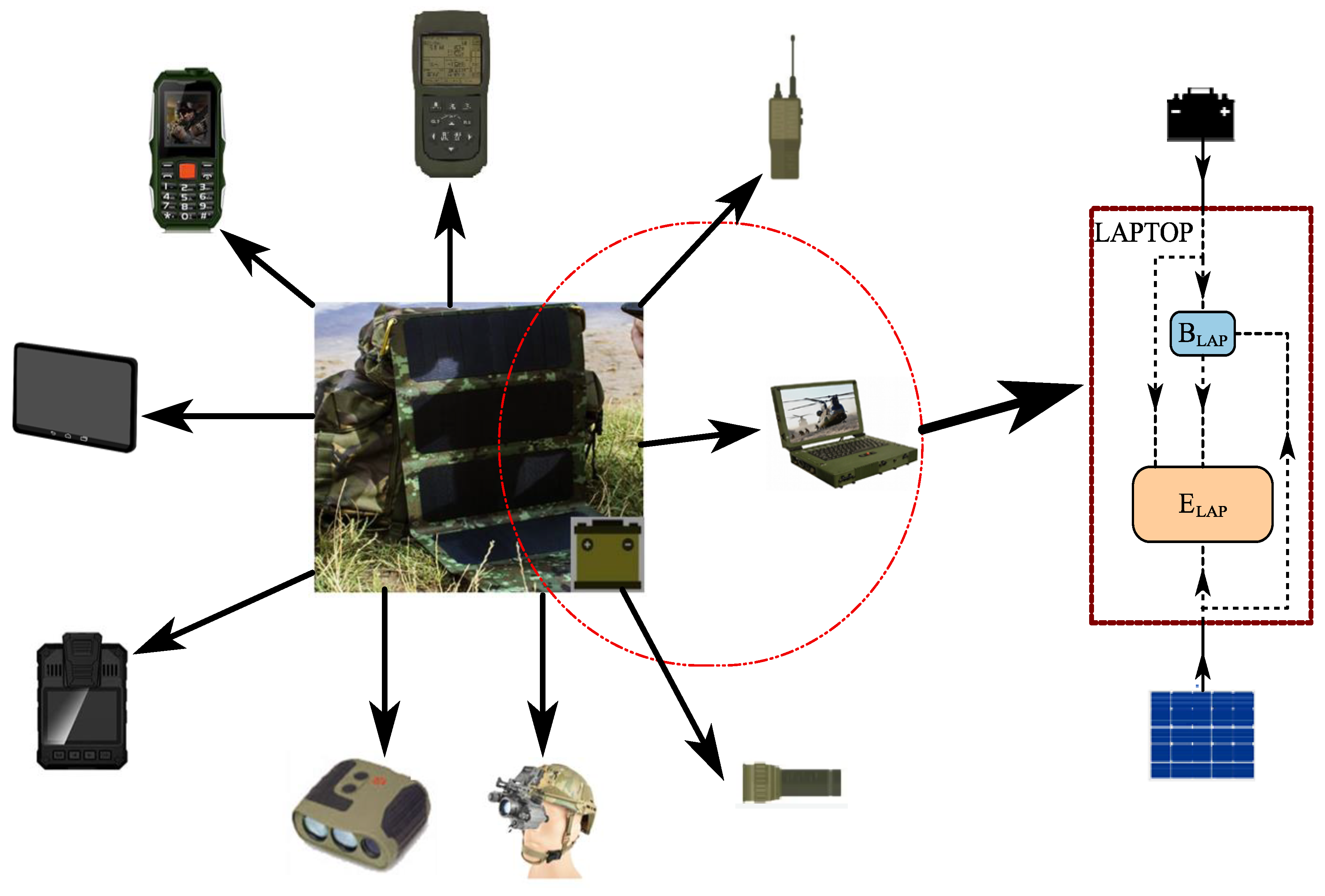
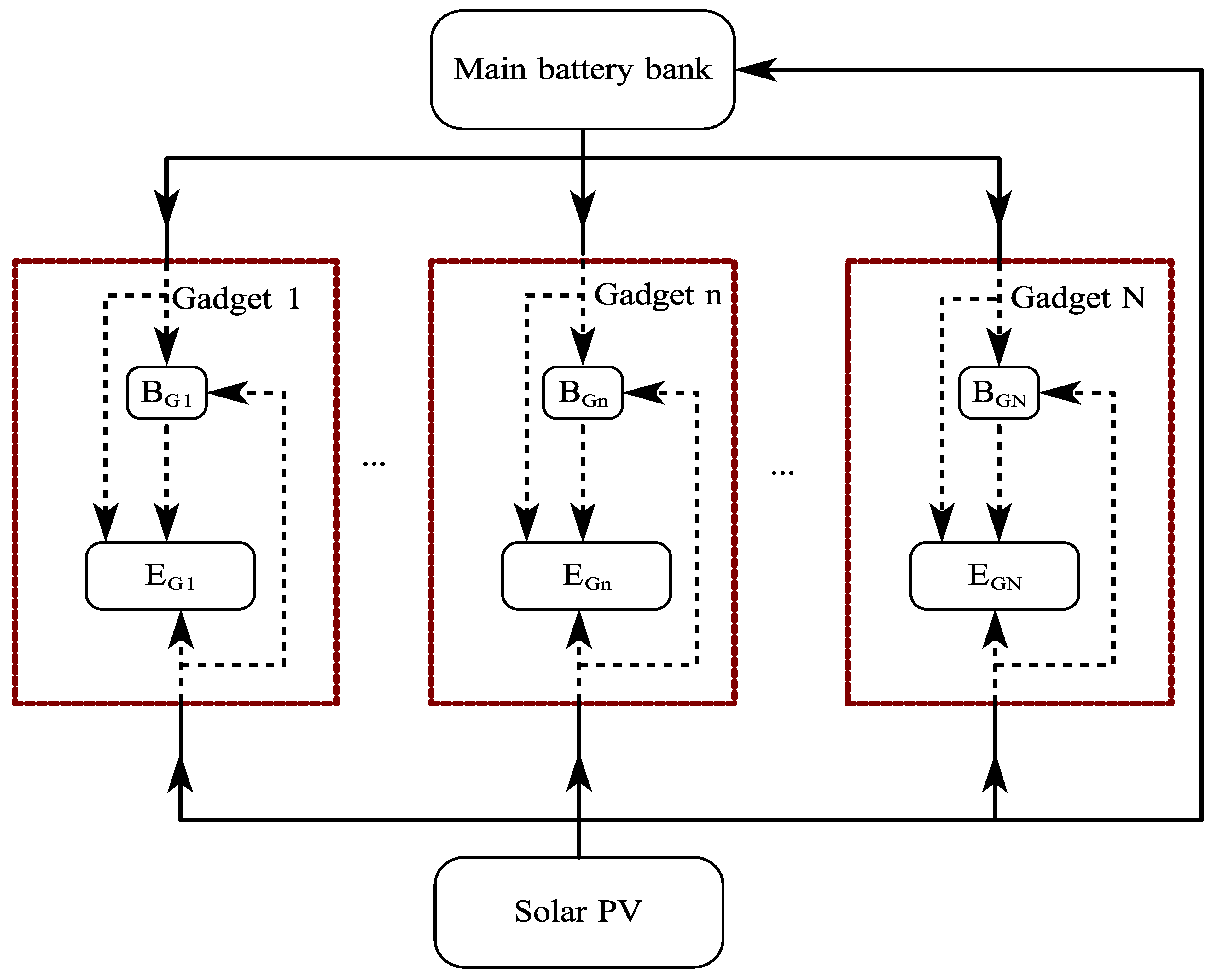
The model developed herein and its accompanying optimisation is flexible and adaptable to any number of PEDs and demand profiles. In this case study, nine soldier-level PEDs (cellphone, GPS, radio, tablet, laptop, torch, MP3 player, night vision, and binoculars) have been used. It is worth noting that real soldier-level PED demand profiles could not be ascertained, as such demand profiles used in this research are randomly generated and also based on the assumption that some devices are only used during the day, some only during the night, and some are used throughout the day. The respective PED demand profiles are as presented in

Table 1. PED power demands (W) for device per hour over 24 h.

Time (h)	Phone	GPS	Radio	Tablet	Laptop	Torch	MP3 Player	Night Vision	Binoculars
1	$0.68$	$1.61$	$1.26$	$1.46$	$0.00$	$1.26$	$0.00$	$2.18$	$1.26$
2	$0.27$	$0.15$	$1.38$	$0.58$	$0.00$	$1.38$	$0.00$	$0.20$	$1.38$
3	$0.63$	$1.34$	$0.37$	$1.35$	$0.00$	$0.37$	$0.00$	$1.82$	$0.37$
4	$0.07$	$1.57$	$1.39$	$0.14$	$0.00$	$1.39$	$0.00$	$2.12$	$1.39$
5	$0.11$	$1.08$	$1.03$	$0.24$	$0.00$	$1.03$	$0.00$	$1.46$	$1.03$
6	$0.46$	$0.55$	$0.33$	$0.99$	$0.00$	$0.33$	$0.00$	$0.74$	$0.33$
7	$0.42$	$0.50$	$0.56$	$0.90$	$0.00$	$0.00$	$0.00$	$0.00$	$0.56$
8	$0.34$	$1.59$	$0.91$	$0.72$	$0.00$	$0.00$	$0.00$	$0.00$	$0.91$
9	$0.28$	$0.44$	$1.45$	$0.59$	$0.00$	$0.00$	$0.00$	$0.00$	$1.45$
10	$0.48$	$0.28$	$1.46$	$1.04$	$0.82$	$0.00$	$0.00$	$0.00$	$1.46$
11	$0.35$	$1.45$	$0.41$	$0.76$	$4.22$	$0.00$	$0.00$	$0.00$	$0.41$
12	$0.56$	$1.97$	$1.47$	$1.21$	$5.75$	$0.00$	$0.00$	$0.00$	$1.47$
13	$0.41$	$0.12$	$1.45$	$0.87$	$0.35$	$0.00$	$0.00$	$0.00$	$1.45$
14	$0.45$	$1.11$	$0.83$	$0.97$	$3.23$	$0.00$	$0.00$	$0.00$	$0.83$
15	$0.50$	$1.69$	$1.24$	$1.07$	$4.95$	$0.00$	$0.00$	$0.00$	$1.24$
16	$0.75$	$1.30$	$0.39$	$1.61$	$3.80$	$0.00$	$0.00$	$0.00$	$0.39$
17	$0.63$	$1.52$	$0.75$	$1.35$	$4.43$	$0.00$	$0.00$	$0.00$	$0.75$
18	$0.33$	$0.68$	$1.40$	$0.71$	$1.98$	$0.00$	$0.00$	$0.00$	$1.40$
19	$0.67$	$1.90$	$1.23$	$1.44$	$5.54$	$1.23$	$1.20$	$2.57$	$1.23$
20	$0.63$	$1.50$	$1.45$	$1.35$	$4.38$	$1.45$	$1.13$	$2.03$	$1.45$
21	$0.07$	$1.17$	$1.06$	$0.15$	$3.40$	$1.06$	$0.13$	$1.58$	$1.06$
22	$0.55$	$0.38$	$0.25$	$1.19$	$0.00$	$0.25$	$0.99$	$0.52$	$0.25$
23	$0.61$	$0.84$	$1.31$	$1.32$	$0.00$	$1.31$	$0.00$	$1.13$	$1.31$
24	$0.57$	$1.42$	$1.42$	$1.22$	$0.00$	$1.42$	$0.00$	$1.93$	$1.42$

.

The respective battery specifications for the PED used in this case study are presented in

Table 2. Battery specifications.

PED	Battery Capacity (mAh)	Battery Voltage (V)
Main battery	20,000	5
Cellphone	2600	5
GPS	5000	$3.7$
Radio	1600	5
Tablet	4000	$10.8$
Laptop	4050	$10.8$
Torch	2600	5
MP3	5000	9
Night vision	5000	5
Binoculars	5000	5

:

Table 3. Case study parameters.

Parameter	Value
Charging efficiency (${\eta }_c$)	$0.9$
Discharging efficiency (${\eta }_d$)	$0.95$
Solar panel efficiency (${\eta }_{sol}$)	$0.22$
Solar PV area ($Ar$)	0.3 m2
Depth of discharge (DOD)	$0.95$
Duration of one-time slot in minutes (T)	60 min
Duration of one-time slot in hours ($\Delta t$)	1  h
Solar irradiance sampling time slot length (N)	24  h
The time it takes to fully charge the PED battery ($\alpha$)	2 h
The time it takes to fully charge the main battery ($\varphi$)	3 h
Incoming solar irradiance factor ($\gamma$) for scenarios 1, 2, 3, and 4, respectively	100%, 50–100%, 25–100%, and  0–50%
Maximum time to continuously charge a battery from zero to full capacity ($\beta$)	12 h

gives the parameters used in this case study and their respective values.

5. Results and Discussion

Figure 5 shows the solar power output considering the shading scenarios. A universal amount of solar radiation amount for a specific day was used across all scenarios as was pointed out in Section 4. In reality, there will not be the same amount of radiation for every hour for all the scenarios owing to varied shading aspects attributed to different seasonal variations, terrains, topography, cloud cover, and shading effects from trees and other obstacles. The modelling and optimisation approach taken was made to mimic the real practical state of things by picking random percentages of solar radiation for each hour accordingly as per each prescribed scenario’s distribution. As such, scenario 1 shows a symmetrical pattern as 100% solar radiation is received for the chosen day in question. Scenarios 2, 3, and 4 do not show symmetrical patterns as these are deviations from scenario 1 which have randomly assigned the optimisation system’s percentage decreases in irradiance which follows no particular order. However, the distributions in the scenarios will be symmetrical on average in terms of the overall power output for the scenarios.

The findings depicted in Figure 5 elucidate a noteworthy correlation between the degree of shading and its consequential impact on power output. As shading increased progressively from 0% in scenario 1 to an average of 75% in scenario 4, a discernible negative effect on power output emerged. The shading phenomenon notably diminished the incident irradiation on the solar cells, consequently leading to a reduction in their power generation capacity. Visualised in Figure 5, scenario 1, characterised by minimal shading, covered a larger area, indicating higher power generation compared to scenarios 2, 3, and 4. The decline in power generation is apparent, with scenario 2 exhibiting lower output than scenario 1, followed by a further reduction in scenario 3 compared to scenario 2. Ultimately, scenario 4 showcased the least power generation, aligning with the escalating degree of shading observed across the scenarios.

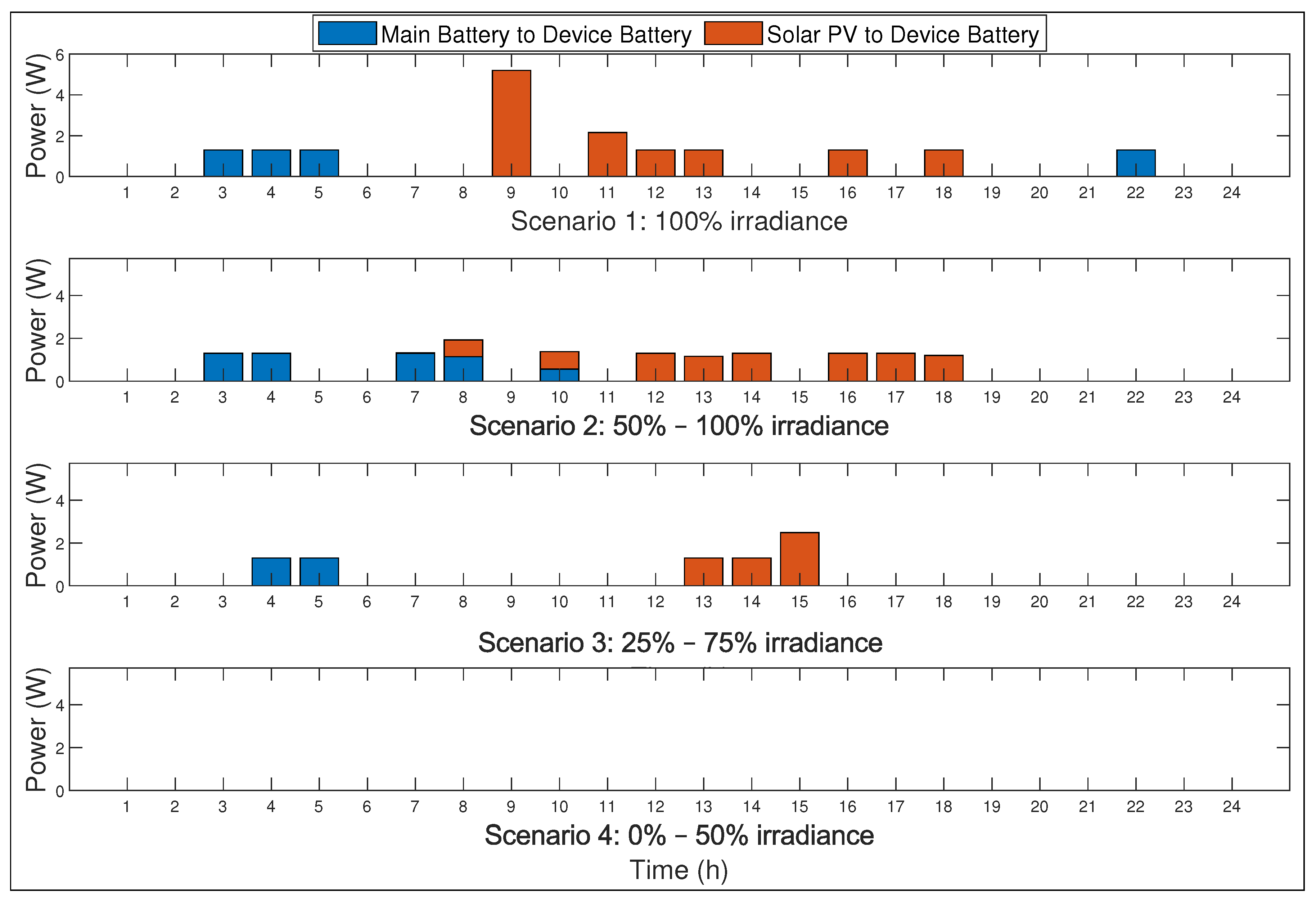
Figure 6 shows the main battery and the solar irradiance charging the PED battery. When it comes to the share of the solar irradiance, it can be seen from scenario 1 that a lot of sun has charged the PED battery more than in other scenarios, in scenario 2 it is seen that the sun still charged the PED battery a lot but less than in scenario 1 and more than in scenarios 3 and 4. In scenario 3, solar PV did not charge the PED battery that much because there was not enough sun. The sun did not charge the PED battery at all in scenario 4 because of the high intensity of shading. The main battery charged the PED battery more in scenario 1 because of the abundant solar insolation available from the solar PV unlike in scenarios 2 and 3 where the incident solar radiation is limited. In scenario 3, both solar PV and the main battery did not charge the PED battery that much as there was too much shading. In scenario 4, the main battery did not charge the PED battery at all owing to itself not having been adequately charged by solar PV in the first place.

Power flows to PED electronics are presented in Figure 7. The bulk of the power to meet the PED electronics demand is supplied by the respective PED battery with fewer instances where solar PV and the main battery supply the PED electronics directly. The share of solar PV and main battery power supply to the PED electronics decreases as we move from scenario 1 to scenario 4 in congruence with the increase in shading percentage increase from scenario 1 through to scenario 4. In all the scenarios in Figure 7, it can be seen that the amount of power supplied to the PED electronics is the same in all the scenarios for the respective hours even though there are variations of the source in a few instances. This is attributed to the fact that there are always similar demands for the respective hours for all the scenarios. Overall, the optimisation guaranteed the consistent satisfaction of demand for PED electronics, utilising a supply derived from the solar PV or the main battery or PED battery or a combination thereof, ensuring continuous availability of power supply.

Figure 8 presents the State of Charge (SoC) for the phone (PED under consideration) battery. For scenario 1, SoC starts lower but based on the fact that there was a lot of energy available, the battery ended up charging more than all the other scenarios. In scenario 2, SoC started at almost the same level as in scenario 1 but it ended up lower than scenario 1, meaning that it did not obtain more charge as compared to scenario 1. SoC for scenario 3 started higher than that of scenarios 1 and 2 but lower than that of scenario 4. For scenario 4, the optimisation system picked that there was not enough solar radiation to charge the main battery and decided to start it on a higher SoC initial level in order to satisfy the objective of meeting the demand by all costs at all times. The SoC trend for scenario 4 shows that the PED battery did not charge at all, which agrees with the result shown in Figure 6 alluding to the unavailability of enough incident solar radiation to boost the energy.

The modelling and optimisation results under discussion are for all nine PEDs. However, due to their similar nature, the graphical results presented in Figure 6, Figure 7 and Figure 8 are for one of the nine PEDs (the phone). The presented results for the phone in the aforementioned figures are typical of the rest of the PEDs used in this study with major differences in the amount and source of power to meet the demand for the respective PED electronics for every hour of the day, amount and source of power to charge the PED batteries for every hour of the day and variation in PED battery levels as depicted by change in state of charge (SoC) for every hour of the day. For further information regarding optimisation results for the rest of the PEDs, the authors refer the reader to

Table A1. Battery state of charge (%).

Time	Cellphone Scenarios				GPS Scenarios				Radio Scenarios				Tablet Scenarios				Laptop Scenarios				Torch Scenarios				MP3 Scenarios				Night Vision Scenarios				Binoculars Scenarios				Main Battery Scenarios
	1	2	3	4	1	2	3	4	1	2	3	4	1	2	3	4	1	2	3	4	1	2	3	4	1	2	3	4	1	2	3	4	1	2	3	4	1	2	3	4
01:00	11.94	11.94	19.67	84.07	34.53	48.08	42.97	95.00	80.83	55.84	72.46	95.00	12.76	36.50	5.00	54.70	6.78	38.52	28.44	95.00	34.53	79.67	32.98	92.09	12.28	12.28	5.00	12.28	74.46	74.46	37.38	74.46	29.29	33.03	37.98	95.00	48.94	86.57	35.38	62.18
02:00	6.97	6.97	14.70	79.10	26.26	39.82	34.71	86.73	95.00	70.01	86.63	80.04	9.55	33.29	14.00	51.49	6.78	38.52	28.44	95.00	25.32	70.47	23.77	82.88	12.28	12.28	5.00	12.28	66.18	66.18	29.09	66.18	24.50	28.24	33.20	90.21	46.54	84.18	27.50	62.18
03:00	5.00	5.00	12.72	77.13	25.49	39.05	33.94	85.96	78.61	85.54	70.24	63.65	8.28	32.01	23.00	50.21	6.78	38.52	28.44	95.00	34.87	60.38	13.68	72.80	12.28	12.28	5.00	12.28	75.18	65.42	28.33	65.42	19.26	23.00	27.95	84.97	41.35	81.55	22.84	62.18
04:00	14.00	14.00	8.12	72.52	18.61	32.16	27.05	79.08	74.22	94.54	65.85	59.26	5.31	29.04	20.03	47.24	6.78	38.52	28.44	95.00	32.17	57.68	22.68	70.10	12.28	12.28	5.00	12.28	68.26	58.50	21.42	58.50	17.85	21.59	26.55	83.56	39.52	78.61	21.25	62.18
05:00	23.00	23.00	17.12	72.01	10.55	24.10	18.99	71.02	57.71	78.03	49.34	42.75	5.00	28.74	19.72	46.94	6.78	38.52	28.44	95.00	22.01	47.52	12.53	59.94	12.28	12.28	5.00	12.28	60.21	50.45	13.36	50.45	12.57	16.31	21.26	78.28	38.22	77.31	19.95	62.18
06:00	32.00	22.20	26.12	71.21	5.00	18.56	27.99	65.47	45.48	65.80	60.93	30.52	14.00	28.21	19.20	46.41	6.78	38.52	28.44	95.00	14.48	56.52	5.00	52.41	12.28	12.28	5.00	12.28	54.66	44.90	7.81	44.90	8.65	12.39	17.35	74.37	32.55	75.09	13.87	62.18
07:00	28.64	18.83	22.76	67.85	12.50	15.73	36.99	62.65	41.56	61.88	57.01	26.60	11.82	26.03	28.20	44.23	6.78	38.52	28.44	95.00	23.48	54.11	14.00	50.00	12.28	12.28	5.00	12.28	51.85	42.09	5.00	42.09	17.65	11.14	16.10	73.11	26.32	75.09	5.00	62.18
08:00	25.57	28.00	19.69	64.78	21.50	13.16	34.42	60.08	49.06	55.23	50.36	19.95	9.84	24.05	26.22	42.25	6.78	38.52	28.44	95.00	32.48	54.11	14.00	50.00	12.28	12.28	5.00	12.28	51.85	42.09	5.00	42.09	15.53	9.01	13.97	70.98	21.76	73.48	5.03	62.18
09:00	23.08	41.35	17.20	62.29	34.56	5.00	26.26	51.92	59.30	44.43	39.56	36.25	20.95	22.47	24.63	40.67	6.78	38.52	28.44	95.00	32.48	54.11	14.00	50.00	12.28	12.28	5.00	12.28	63.30	42.09	5.00	42.09	12.07	5.55	10.51	67.53	13.21	72.40	7.14	60.66
10:00	59.08	39.30	15.16	60.25	69.00	14.00	24.00	49.66	42.08	27.21	22.34	19.04	19.66	21.17	23.34	39.37	6.78	38.52	28.44	95.00	32.48	54.11	14.00	50.00	12.28	12.28	5.00	12.28	63.30	42.09	5.00	42.09	6.56	13.70	5.00	62.02	20.37	77.18	12.61	60.66
11:00	55.58	48.87	11.65	56.74	67.56	24.44	22.56	48.22	24.74	9.87	5.00	64.04	18.75	20.27	22.43	38.47	5.00	36.74	26.65	93.22	32.48	54.11	14.00	50.00	12.28	12.28	5.00	12.28	63.30	42.09	5.00	42.09	5.00	12.14	30.79	60.46	51.64	76.37	18.92	55.48
12:00	70.55	46.31	9.09	54.18	60.12	16.99	15.12	40.77	60.74	5.00	22.46	59.17	17.08	18.60	30.54	36.80	14.00	45.43	17.49	84.05	77.48	54.11	14.00	50.00	57.28	12.28	5.00	12.28	72.30	42.09	5.00	42.09	14.75	10.59	69.45	58.90	49.07	93.12	16.67	55.48
13:00	79.55	55.31	5.00	50.09	50.00	6.88	5.00	30.66	43.29	22.22	5.00	41.71	26.08	63.60	27.88	34.14	25.83	57.26	5.00	71.56	77.48	54.11	14.00	50.00	57.28	12.28	5.00	12.28	72.30	42.09	5.00	42.09	23.75	5.00	63.87	53.31	78.03	93.12	50.84	77.27
14:00	88.55	63.32	14.00	47.09	95.00	15.88	50.00	75.66	68.60	5.00	21.31	86.71	24.17	61.69	36.88	32.22	34.83	56.50	21.35	80.56	77.48	54.11	34.28	50.00	57.28	12.28	14.00	12.28	72.30	42.09	50.00	42.09	37.97	14.00	58.36	47.80	72.79	93.12	46.69	65.73
15:00	85.26	72.32	23.00	43.80	89.30	24.88	44.30	69.96	58.74	17.92	49.59	76.85	22.04	59.55	34.75	30.09	27.82	49.48	35.94	73.55	77.48	54.11	34.28	50.00	57.28	12.28	14.00	12.28	72.30	42.09	50.00	42.09	34.82	59.00	72.07	44.65	87.36	92.46	42.05	65.73
16:00	81.60	68.67	40.15	40.15	80.62	41.00	56.68	61.28	44.02	50.27	63.54	62.13	19.68	57.20	32.40	27.74	38.00	38.73	25.19	62.80	77.48	54.11	43.28	50.00	57.28	12.28	14.00	12.28	72.30	42.09	95.00	42.09	72.68	68.00	67.36	39.94	84.98	92.46	41.58	65.73
17:00	90.60	77.67	34.67	34.67	73.95	86.00	50.00	54.60	57.41	59.27	58.90	57.50	28.68	86.00	28.86	24.20	29.75	30.48	16.94	54.55	77.48	54.11	43.28	50.00	57.28	12.28	14.00	12.28	72.30	42.09	95.00	42.09	81.68	77.00	65.88	38.46	84.22	95.00	63.07	76.74
18:00	86.00	86.67	30.07	30.07	66.14	95.00	95.00	46.80	71.41	50.37	67.90	48.59	25.71	95.00	25.89	21.23	74.75	20.86	38.53	44.92	77.48	54.11	43.28	50.00	57.28	12.28	14.00	12.28	72.30	42.09	95.00	42.09	78.83	74.15	95.00	35.61	83.17	95.00	49.94	89.62
19:00	95.00	95.00	27.65	27.65	62.65	91.51	91.51	43.31	87.16	95.00	51.28	31.97	24.15	93.44	24.33	19.67	70.45	33.93	34.23	40.62	77.48	54.11	43.28	50.00	57.28	12.28	14.00	12.28	72.30	42.09	95.00	42.09	73.51	83.15	89.68	30.29	95.00	90.84	59.27	95.00
20:00	90.10	90.10	22.76	22.76	52.89	81.75	81.75	33.55	72.55	80.39	36.67	76.97	34.93	90.27	21.16	16.50	58.41	21.90	22.20	28.59	95.00	45.12	34.29	95.00	54.75	23.68	11.47	9.75	62.54	32.32	85.23	32.32	82.51	78.48	85.01	25.61	85.56	86.57	61.22	83.76
21:00	85.50	85.50	18.15	18.15	45.19	74.05	74.05	25.85	55.33	63.18	19.45	59.75	43.93	87.30	18.19	13.53	48.90	12.38	12.68	37.60	84.40	34.52	23.70	84.40	52.36	21.30	9.08	7.36	54.82	24.61	77.52	24.61	77.00	72.97	79.50	70.61	80.17	86.57	61.22	62.18
22:00	84.99	84.99	17.64	17.64	54.19	68.04	68.04	19.84	67.26	50.59	6.87	47.16	52.93	86.97	25.69	13.20	41.52	5.00	21.68	30.22	76.66	26.78	15.95	76.66	52.09	21.02	8.81	7.09	48.82	18.60	71.52	18.60	86.00	68.94	75.47	66.58	67.66	86.57	50.28	62.18
23:00	93.99	80.97	13.62	13.62	63.19	66.09	66.09	17.89	64.29	47.62	15.87	44.19	50.32	84.36	23.07	10.59	41.52	5.00	21.68	30.22	85.66	24.95	24.95	74.83	50.00	18.93	6.72	5.00	56.32	16.63	69.54	16.63	95.00	67.99	74.52	65.63	57.23	86.57	47.81	62.18
24:00	89.53	76.51	9.17	9.17	58.88	61.78	61.78	13.57	79.03	32.06	30.60	28.64	47.41	81.45	32.07	7.68	41.52	5.00	21.68	30.22	76.08	15.38	15.38	65.26	50.00	18.93	6.72	5.00	52.02	12.33	65.25	12.33	90.02	63.01	69.54	60.66	54.74	86.57	39.96	62.18

,

Table A2. Solar PV to PED batteries (W).

Time	Cellphone Scenarios				GPS Scenarios				Radio Scenarios				Tablet Scenarios				Laptop Scenarios				Torch Scenarios				MP3 Scenarios				Night Vision Scenarios				Binoculars Scenarios
	1	2	3	4	1	2	3	4	1	2	3	4	1	2	3	4	1	2	3	4	1	2	3	4	1	2	3	4	1	2	3	4	1	2	3	4
01:00	0	0	0	0	0	0	0	0	0	0	0	0	0	0	0	0	0	0	0	0	0	0	0	0	0	0	0	0	0	0	0	0	0	0	0	0
02:00	0	0	0	0	0	0	0	0	0	0	0	0	0	0	0	0	0	0	0	0	0	0	0	0	0	0	0	0	0	0	0	0	0	0	0	0
03:00	0	0	0	0	0	0	0	0	0	0	0	0	0	0	0	0	0	0	0	0	0	0	0	0	0	0	0	0	0	0	0	0	0	0	0	0
04:00	0	0	0	0	0	0	0	0	0	0	0	0	0	0	0	0	0	0	0	0	0	0	0	0	0	0	0	0	0	0	0	0	0	0	0	0
05:00	0	0	0	0	0	0	0	0	0	0	0	0	0	0	0	0	0	0	0	0	0	0	0	0	0	0	0	0	0	0	0	0	0	0	0	0
06:00	0	0	0	0	0	0	0	0	0	0	0	0	0	0	0	0	0	0	0	0	0	0	0	0	0	0	0	0	0	0	0	0	0	0	0	0
07:00	0	0.02	0	0	0	0	0	0	0.07	0	0	0	0	0	0	0	0	0	0	0	0	0	0	0	0	0	0	0	0	0	0	0	0	0	0	0
08:00	0	0.78	0	0	0.83	0	0	0	0.91	0	0	0.65	1.27	0	0	0	0	0	0	0	0	0	0	0	0	0	0	0	0.85	0	0	0	0	0	0	0
09:00	5.2	0	0	0	7.08	1.85	0	0	0	0	0	0	0	0		0	0	0	0	0	0	0	0	0	0	0	0	0	0	0	0	0	0	2.26	0	0
10:00	0	0.82	0	0	0	1.85	0	0	0	0	0	0	0	0	0	0	0	0	0	0	0	0	0	0	0	0	0	0	0	0	0	0	0	0	7.16	0
11:00	2.16	0	0	0	0	0	0	0	3.2	0	1.55	0	0	0	1.52	0	4.37	4.22	0	0	6.5	0	0	0	22.5	0	0	0	2.5	0	0	0	0.21	0	10.74	0
12:00	1.3	1.3	0	0	0	0	0	0	0	1.53	0	0	4.32	21.6	0	0	5.75	5.75	0	0	0	0	0	0	0	0	0	0	0	0	0	0	2.5	0	0	0
13:00	1.3	1.16	1.3	0	7.04	1.85	9.25	7.4	1.45	0	1.45	0	0	0	4.32	0	4.37	0	3.57	0	0	0	2.93	0	0	0	4.5	0	0	0	12.5	0	1.45	2.5	0	0
14:00	0	1.3	1.3	0	0	1.85	0	0	0	0.8	2.51	0	0	0	0	0	0	0	2.72	0	0	0	0	0	0	0	0	0	0	0	0	0	0	12.5	3.81	0
15:00	0	0	2.48	0	0	3.31	2.54	0	0	2.88	0.99	0	0	0	0	0	4.95	0	0	0	0	0	1.3	0	0	0	0	0	0	0	12.5	0	8.02	2.5	0	0
16:00	1.3	1.3	0	0	0	9.25	0	0	0.39	0.8	0	0	4.32	13.82	0	0	0	0	0	0	0	0	0	0	0	0	0	0	0	0	0	0	2.5	2.5	0	0
17:00	0	1.3	0	0	0	1.85	9.25	0	0.44	0	0.8	0	0	4.32	0	0	21.87	0	0.55	0	0	0	0	0	0	0	0	0	0	0	0	0	0	0	8.09	0
18:00	1.3	1.2	0	0	0	0	0	0	1.4	3.97	0	0	0	0	0	0	0	1.98	0	0	0	0	0	0	0	0	0	0	0	0	0	0	0	2.5	0	0
19:00	0	0	0	0	0	0	0	0	0	0	0	1.13	0.85	0	0	0	0	0	0	0	1.23	0	0	0	0	1.2	0	0	0	0	0	0	0	0	0	0
20:00	0	0	0	0	0	0	0	0	0	0	0	0	0	0	0	0	0	0	0	0	0	0	0	0	0	0	0	0	0	0	0	0	0	0	0	0
21:00	0	0	0	0	0	0	0	0	0	0	0	0	0	0	0	0	0	0	0	0	0	0	0	0	0	0	0	0	0	0	0	0	0	0	0	0
22:00	0	0	0	0	0	0	0	0	0	0	0	0	0	0	0	0	0	0	0	0	0	0	0	0	0	0	0	0	0	0	0	0	0	0	0	0
23:00	0	0	0	0	0	0	0	0	0	0	0	0	0	0	0	0	0	0	0	0	0	0	0	0	0	0	0	0	0	0	0	0	0	0	0	0
24:00	0	0	0	0	0	0	0	0	0	0	0	0	0	0	0	0	0	0	0	0	0	0	0	0	0	0	0	0	0	0	0	0	0	0	0	0

,

Table A3. Main battery to PED battery (W).

Time	Cellphone Scenarios				GPS Scenarios				Radio Scenarios				Tablet Scenarios				Laptop Scenarios				Torch Scenarios				MP3 Scenarios				Night Vision Scenarios				Binoculars Scenarios
	1	2	3	4	1	2	3	4	1	2	3	4	1	2	3	4	1	2	3	4	1	2	3	4	1	2	3	4	1	2	3	4	1	2	3	4
01:00	0	0	0	0	0	0	0	0	1.26	1.26	1.26	0	0	0	4.32	0	0	0	0	0	0	0	0	0	0	0	0	0	0	0	0	0	0	0	0	0
02:00	0	0	0	0	0	0	0	0	0	1.38	0	0	0	0	4.32	0	0	0	0	0	1.38	0	0	0	0	0	0	0	2.5	0	0	0	0	0	0	0
03:00	1.3	1.3	0	0	0	0	0	0	0	0.8	0	0	0	0	0	0	0	0	0	0	0	0	1.3	0	0	0	0	0	0	0	0	0	0	0	0	0
04:00	1.3	1.3	1.3	0	0	0	0	0	0	0	0	0	0	0	0	0	0	0	0	0	0	0	0	0	0	0	0	0	0	0	0	0	0	0	0	0
05:00	1.3	0	1.3	0	0	0	1.85	0	0	0	1.03	0	4.32	0	0	0	0	0	0	0	0	1.3	0	0	0	0	0	0	0	0	0	0	0	0	0	0
06:00	0	0	0	0	1.54	0	1.85	0	0	0	0	0	0	0	4.32	0	0	0	0	0	1.3	0	1.3	0	0	0	0	0	0	0	0	0	2.5	0	0	0
07:00	0	1.3	0	0	1.85	0	0	0	0.6	0	0	0	0	0	0	0	0	0	0	0	1.3	0	0	0	0	0	0	0	0	0	0	0	0	0	0	0
08:00	0	1.14	0	0	1.85	0	0	0	0	0	0	0.8	4.07	0	0	0	0	0	0	0	0	0	0	0	0	0	0	0	2.33	0	0	0	0	0	0	0
09:00	0	0	0	0	0	0	0	0	0	0	0	0	0	0	0	0	0	0	0	0	0	0	0	0	0	0	0	0	0	0	0	0	0	0	0	0
10:00	0	0.56	0	0	0	0.3	0	0	0	0	0	4	0	0	0	0	0	0	0	0	0	0	0	0	0	0	0	0	0	0	0	0	0	0	0	0
11:00	0	0	0	0	0	0	0	0	0	0	0	0	0	0	2.38	0	0	0	0	0	0	0	0	0	0	0	0	0	0	0	0	0	2.5	0	0	0
12:00	0	0	0	0	0	0	0	0	0	0	0	0	0	0	0	0	0	0	0	0	0	0	0	0	0	0	0	0	0	0	0	0	0	0	0	0
13:00	0	0	0	0	2.21	0	0	1.85	0.8	0	0	4	0	0	0	0	0	0	4.37	4.37	0	0	0	0	0	0	0	0	0	0	0	0	2.5	0	0	0
14:00	0	0	0	0	0	0	0	0	0	0.35	0	0	0	0	0	0	0	0	4.37	0	0	0	0	0	0	0	0	0	0	0	0	0	0	0	0	0
15:00	0	0	0	0	0	0	0	0	0	0	0.25	0	0	0	0	0	0	0	0	0	0	0	0	0	0	0	0	0	0	0	0	0	2.5	0	0	0
16:00	0	0	0	0	0	0	0	0	0.8	0	0	0	0	0	0	0	0	0	0	0	0	0	0	0	0	0	0	0	0	0	0	0	0	0	0	0
17:00	0	0	0	0	0	0	0	0	0.8	0	0	0	0	0	0	0	0	0	9.94	0	0	0	0	0	0	0	0	0	0	0	0	0	0	0	0	0
18:00	0	0	0	0	0	0	0	0	0	0	0	0	0	0	0	0	0	4.37	0	0	0	0	0	0	0	0	0	0	0	0	0	0	0	0	0	0
19:00	0	0	0	0	0	0	0	0	0	0	0	2.87	4.32	0	0	0	0	0	0	0	1.3	0	0	6.5	0	4.5	0	0	0	0	0	0	2.5	0	0	0
20:00	0	0	0	0	0	0	0	0	0	0	0	0	4.32	0	0	0	0	0	0	4.38	0	0	0	0	0	0	0	0	0	0	0	0	0	0	0	12.5
21:00	0	0	0	0	1.85	0	0	0	1.06	0	0	0	4.32	0	3.6	0	0	0	4.37	0	0	0	0	0	0	0	0	0	0	0	0	0	2.5	0	0	0
22:00	1.3	0	0	0	1.85	0	0	0	0	0	0.8	0	0	0	0	0	0	0	0	0	1.3	0	1.3	0	0	0	0	0	2.08	0	0	0	2.5	0	0	0
23:00	0	0	0	0	0	0	0	0	1.31	0	1.31	0	0	0	4.32	0	0	0	0	0	0	0	0	0	0	0	0	0	0	0	0	0	0	0	0	0
24:00	0	0	0	0	1.85	0	0	0	1.42	0	0	0	0	0	3.6	0	0	0	0	0	0	0	0	0	0	0	0	0	0	0	0	0	0	0	0	0

,

Table A4. Solar PV to PED electronics (W).

Time	Cellphone Scenarios				GPS Scenarios				Radio Scenarios				Tablet Scenarios				Laptop Scenarios				Torch Scenarios				MP3 Scenarios				Night Vision Scenarios				Binoculars Scenarios
	1	2	3	4	1	2	3	4	1	2	3	4	1	2	3	4	1	2	3	4	1	2	3	4	1	2	3	4	1	2	3	4	1	2	3	4
01:00	0	0	0	0	0	0	0	0	0	0	0	0	0	0	0	0	0	0	0	0	0	0	0	0	0	0	0	0	0	0	0	0	0	0	0	0
02:00	0	0	0	0	0	0	0	0	0	0	0	0	0	0	0	0	0	0	0	0	0	0	0	0	0	0	0	0	0	0	0	0	0	0	0	0
03:00	0	0	0	0	0	0	0	0	0	0	0	0	0	0	0	0	0	0	0	0	0	0	0	0	0	0	0	0	0	0	0	0	0	0	0	0
04:00	0	0	0	0	0	0	0	0	0	0	0	0	0	0	0	0	0	0	0	0	0	0	0	0	0	0	0	0	0	0	0	0	0	0	0	0
05:00	0	0	0	0	0	0	0	0	0	0	0	0	0	0	0	0	0	0	0	0	0	0	0	0	0	0	0	0	0	0	0	0	0	0	0	0
06:00	0	0	0	0	0	0	0	0	0	0	0	0	0	0	0	0	0	0	0	0	0	0	0	0	0	0	0	0	0	0	0	0	0	0	0	0
07:00	0	0.02	0	0	0	0	0	0	0	0	0	0	0	0	0	0	0	0	0	0	0	0	0	0	0	0	0	0	0	0	0	0	0	0	0	0
08:00	0	0.34	0	0	0.83	0	0	0	0.91	0	0	0.11	0.72	0	0	0	0	0	0	0	0	0	0	0	0	0	0	0	0	0	0	0	0	0	0	0
09:00	0.28	0	0	0	0.44	0.44	0	0	0	0	0	0	0	0	0	0	0	0	0	0	0	0	0	0	0	0	0	0	0	0	0	0	0	1.45	0	0
10:00	0	0.48	0	0	0	0.28	0	0	0	0	0	0	0	0	0	0	0	0	0	0	0	0	0	0	0	0	0	0	0	0	0	0	0	0	0.41	0
11:00	0.35	0	0	0	0	0	0	0	0.41	0	0.41	0	0	0	0.76	0	4.22	4.22	0	0	0	0	0	0	0	0	0	0	0	0	0	0	0.21	0	0.41	0
12:00	0.56	0.56	0	0	0	0	0	0	0	1.47	0	0	1.21	1.21	0	0	5.75	5.75	0	0	0	0	0	0	0	0	0	0	0	0	0	0	1.47	0	0	0
13:00	0.41	0.41	0.41	0	0.12	0.12	0.12	0	1.45	0	1.45	0	0	0	0.87	0	0.35	0	0.35	0	0	0	0	0	0	0	0	0	0	0	0	0	1.45	1.45	0	0
14:00	0	0.45	0.45	0	0	1.11	0	0	0	0.48	0.83	0	0	0	0	0	0	0	2.72	0	0	0	0	0	0	0	0	0	0	0	0	0	0	0.83	0.83	0
15:00	0	0	0.5	0	0	1.69	1.69	0	0	1.24	0.99	0	0	0	0	0	4.95	0	0	0	0	0	0	0	0	0	0	0	0	0	0	0	1.24	1.24	0	0
16:00	0.75	0.75	0	0	0	1.3	0	0	0.39	0.39	0	0	1.61	1.61	0	0	0	0	0	0	0	0	0	0	0	0	0	0	0	0	0	0	0.39	0.39	0	0
17:00	0	0.63	0	0	0	1.52	1.52	0	0.44	0	0.75	0	0	1.35	0	0	4.43	0	0.55	0	0	0	0	0	0	0	0	0	0	0	0	0	0	0	0.75	0
18:00	0.33	0.33	0	0	0	0	0	0	1.4	1.4	0	0	0	0	0	0	0	1.98	0	0	0	0	0	0	0	0	0	0	0	0	0	0	0	1.4	0	0
19:00	0	0	0	0	0	0	0	0	0	0	0	0	0.85	0	0	0	0	0	0	0	1.23	0	0	0	0	1.2	0	0	0	0	0	0	0	0	0	0
20:00	0	0	0	0	0	0	0	0	0	0	0	0	0	0	0	0	0	0	0	0	0	0	0	0	0	0	0	0	0	0	0	0	0	0	0	0
21:00	0	0	0	0	0	0	0	0	0	0	0	0	0	0	0	0	0	0	0	0	0	0	0	0	0	0	0	0	0	0	0	0	0	0	0	0
22:00	0	0	0	0	0	0	0	0	0	0	0	0	0	0	0	0	0	0	0	0	0	0	0	0	0	0	0	0	0	0	0	0	0	0	0	0
23:00	0	0	0	0	0	0	0	0	0	0	0	0	0	0	0	0	0	0	0	0	0	0	0	0	0	0	0	0	0	0	0	0	0	0	0	0
24:00	0	0	0	0	0	0	0	0	0	0	0	0	0	0	0	0	0	0	0	0	0	0	0	0	0	0	0	0	0	0	0	0	0	0	0	0

,

Table A5. Main battery to PED electronics (W).

Time	Cellphone Scenarios				GPS Scenarios				Radio Scenarios				Tablet Scenarios				Laptop Scenarios				Torch Scenarios				MP3 Scenarios				Night Vision Scenarios				Binoculars Scenarios
	1	2	3	4	1	2	3	4	1	2	3	4	1	2	3	4	1	2	3	4	1	2	3	4	1	2	3	4	1	2	3	4	1	2	3	4
01:00	0	0	0	0	0	0	0	0	1.26	1.26	1.26	0	0	0	1.46	0	0	0	0	0	0	0	0	0	0	0	0	0	0	0	0	0	0	0	0	0
02:00	0	0	0	0	0	0	0	0	0	1.38	0	0	0	0	0.58	0	0	0	0	0	1.38	0	0	0	0	0	0	0	0.2	0	0	0	0	0	0	0
03:00	0.63	0.63	0	0	0	0	0	0	0	0.37	0	0	0	0	0	0	0	0	0	0	0	0	0.37	0	0	0	0	0	0	0	0	0	0	0	0	0
04:00	0.07	0.07	0.07	0	0	0	0	0	0	0	0	0	0	0	0	0	0	0	0	0	0	0	0	0	0	0	0	0	0	0	0	0	0	0	0	0
05:00	0.11	0	0.11	0	0	0	1.08	0	0	0	1.03	0	0.24	0	0	0	0	0	0	0	0	1.03	0	0	0	0	0	0	0	0	0	0	0	0	0	0
06:00	0	0	0	0	0.55	0	0.55	0	0	0	0	0	0	0	0.99	0	0	0	0	0	0.33	0	0.33	0	0	0	0	0	0	0	0	0	0.33	0	0	0
07:00	0	0.4	0	0	0.5	0	0	0	0.56	0	0	0	0	0	0	0	0	0	0	0	0	0	0	0	0	0	0	0	0	0	0	0	0	0	0	0
08:00	0	0	0	0	0.76	0	0	0	0	0	0	0.8	0	0	0	0	0	0	0	0	0	0	0	0	0	0	0	0	0	0	0	0	0	0	0	0
09:00	0	0	0	0	0	0	0	0	0	0	0	0	0	0	0	0	0	0	0	0	0	0	0	0	0	0	0	0	0	0	0	0	0	0	0	0
10:00	0	0	0	0	0	0	0	0	0	0	0	1.46	0	0	0	0	0	0	0	0	0	0	0	0	0	0	0	0	0	0	0	0	0	0	0	0
11:00	0	0	0	0	0	0	0	0	0	0	0	0	0	0	0	0	0	0	0	0	0	0	0	0	0	0	0	0	0	0	0	0	0.2	0	0	0
12:00	0	0	0	0	0	0	0	0	0	0	0	0	0	0	0	0	0	0	0	0	0	0	0	0	0	0	0	0	0	0	0	0	0	0	0	0
13:00	0	0	0	0	0	0	0	0.12	0	0	0	1.45	0	0	0	0	0	0	0	0.35	0	0	0	0	0	0	0	0	0	0	0	0	0	0	0	0
14:00	0	0	0	0	0	0	0	0	0	0.35	0	0	0	0	0	0	0	0	0.51	0	0	0	0	0	0	0	0	0	0	0	0	0	0	0	0	0
15:00	0	0	0	0	0	0	0	0	0	0	0.25	0	0	0	0	0	0	0	0	0	0	0	0	0	0	0	0	0	0	0	0	0	0	0	0	0
16:00	0	0	0	0	0	0	0	0	0	0	0	0	0	0	0	0	0	0	0	0	0	0	0	0	0	0	0	0	0	0	0	0	0	0	0	0
17:00	0	0	0	0	0	0	0	0	0.31	0	0	0	0	0	0	0	0	0	3.88	0	0	0	0	0	0	0	0	0	0	0	0	0	0	0	0	0
18:00	0	0	0	0	0	0	0	0	0	0	0	0	0	0	0	0	0	0	0	0	0	0	0	0	0	0	0	0	0	0	0	0	0	0	0	0
19:00	0	0	0	0	0	0	0	0	0	0	0	1.23	0.59	0	0	0	0	0	0	0	0	0	0	1.23	0	0	0	0	0	0	0	0	1.23	0	0	0
20:00	0	0	0	0	0	0	0	0	0	0	0	0	1.35	0	0	0	0	0	0	4.38	0	0	0	0	0	0	0	0	0	0	0	0	0	0	0	1.45
21:00	0	0	0	0	1.17	0	0	0	1.06	0	0	0	0.15	0	0.15	0	0	0	3.4	0	0	0	0	0	0	0	0	0	0	0	0	0	1.06	0	0	0
22:00	0.55	0	0	0	0.38	0	0	0	0	0	0.25	0	0	0	0	0	0	0	0	0	0.25	0	0.25	0	0	0	0	0	0.52	0	0	0	0.25	0	0	0
23:00	0	0	0	0	0	0	0	0	1.31	0	1.31	0	0	0	1.32	0	0	0	0	0	0	0	0	0	0	0	0	0	0	0	0	0	0	0	0	0
24:00	0	0	0	0	1.42	0	0	0	1.42	0	0	0	0	0	1.22	0	0	0	0	0	0	0	0	0	0	0	0	0	0	0	0	0	0	0	0	0

and

Table A6. PED battery to PED electronics (W).

Time	Cellphone Scenarios				GPS Scenarios				Radio Scenarios				Tablet Scenarios				Laptop Scenarios				Torch Scenarios				MP3 Scenarios				Night Vision Scenarios				Binoculars Scenarios
	1	2	3	4	1	2	3	4	1	2	3	4	1	2	3	4	1	2	3	4	1	2	3	4	1	2	3	4	1	2	3	4	1	2	3	4
01:00	0.68	0.68	0.68	0.68	1.61	1.61	1.61	1.61	0	0	0	1.26	1.46	1.46	0	1.46	0	0	0	0	1.26	1.26	1.26	1.26	0	0	0	0	2.18	2.18	2.18	2.18	1.26	1.26	1.26	1.26
02:00	0.27	0.27	0.27	0.27	0.15	0.15	0.15	0.15	1.38	0	1.38	1.38	0.58	0.58	0	0.58	0	0	0	0	0	1.38	1.38	1.38	0	0	0	0	0	0.2	0.2	0.2	1.38	1.38	1.38	1.38
03:00	0	0	0.63	0.63	1.34	1.34	1.34	1.34	0.37	0	0.37	0.37	1.35	1.35	1.35	1.35	0	0	0	0	0.37	0.37	0	0.37	0	0	0	0	1.82	1.82	1.82	1.82	0.37	0.37	0.37	0.37
04:00	0	0	0	0.07	1.57	1.57	1.57	1.57	1.39	1.39	1.39	1.39	0.14	0.14	0.14	0.14	0	0	0	0	1.39	1.39	1.39	1.39	0	0	0	0	2.12	2.12	2.12	2.12	1.39	1.39	1.39	1.39
05:00	0	0.11	0	0.11	1.08	1.08	0	1.08	1.03	1.03	0	1.03	0	0.24	0.24	0.24	0	0	0	0	1.03	0	1.03	1.03	0	0	0	0	1.46	1.46	1.46	1.46	1.03	1.03	1.03	1.03
06:00	0.46	0.46	0.46	0.46	0	0.55	0	0.55	0.33	0.33	0.33	0.33	0.99	0.99	0	0.99	0	0	0	0	0	0.33	0	0.33	0	0	0	0	0.74	0.74	0.74	0.74	0	0.33	0.33	0.33
07:00	0.42	0	0.42	0.42	0	0.5	0.5	0.5	0	0.56	0.56	0.56	0.9	0.9	0.9	0.9	0	0	0	0	0	0	0	0	0	0	0	0	0	0	0	0	0.56	0.56	0.56	0.56
08:00	0.34	0	0.34	0.34	0	1.59	1.59	1.59	0	0.91	0.91	0	0	0.72	0.72	0.72	0	0	0	0	0	0	0	0	0	0	0	0	0	0	0	0	0.91	0.91	0.91	0.91
09:00	0	0.28	0.28	0.28	0	0	0.44	0.44	1.45	1.45	1.45	1.45	0.59	0.59	0.59	0.59	0	0	0	0	0	0	0	0	0	0	0	0	0	0	0	0	1.45	0	1.45	1.45
10:00	0.48	0	0.48	0.48	0.28	0	0.28	0.28	1.46	1.46	1.46	0	0.41	0.41	0.41	0.41	0.82	0.82	0.82	0.82	0	0	0	0	0	0	0	0	0	0	0	0	0.41	0.41	0	0.41
11:00	0	0.35	0.35	0.35	1.45	1.45	1.45	1.45	0	0.41	0	0.41	0.76	0.76	0	0.76	0	0	4.22	4.22	0	0	0	0	0	0	0	0	0	0	0	0	0	0.41	0	0.41
12:00	0	0	0.56	0.56	1.97	1.97	1.97	1.97	1.47	0	1.47	1.47	0	0	1.21	1.21	0	0	5.75	5.75	0	0	0	0	0	0	0	0	0	0	0	0	0	1.47	1.47	1.47
13:00	0	0	0	0.41	0	0	0	0	0	1.45	0	0	0.87	0.87	0	0.87	0	0.35	0	0	0	0	0	0	0	0	0	0	0	0	0	0	0	0	1.45	1.45
14:00	0.45	0	0	0.45	1.11	0	1.11	1.11	0.83	0	0	0.83	0.97	0.97	0.97	0.97	3.23	3.23	0	3.23	0	0	0	0	0	0	0	0	0	0	0	0	0.83	0	0	0.83
15:00	0.5	0.5	0	0.5	1.69	0	0	1.69	1.24	0	0	1.24	1.07	1.07	1.07	1.07	0	4.95	4.95	4.95	0	0	0	0	0	0	0	0	0	0	0	0	0	0	1.24	1.24
16:00	0	0	0.75	0.75	1.3	0	1.3	1.3	0	0	0.39	0.39	0	0	1.61	1.61	3.8	3.8	3.8	3.8	0	0	0	0	0	0	0	0	0	0	0	0	0	0	0.39	0.39
17:00	0.63	0	0.63	0.63	1.52	0	0	1.52	0	0.75	0	0.75	1.35	0	1.35	1.35	0	4.43	0	4.43	0	0	0	0	0	0	0	0	0	0	0	0	0.75	0.75	0	0.75
18:00	0	0	0.33	0.33	0.68	0.68	0.68	0.68	0	0	1.4	1.4	0.71	0.71	0.71	0.71	1.98	0	1.98	1.98	0	0	0	0	0	0	0	0	0	0	0	0	1.4	0	1.4	1.4
19:00	0.67	0.67	0.67	0.67	1.9	1.9	1.9	1.9	1.23	1.23	1.23	0	0	1.44	1.44	1.44	5.54	5.54	5.54	5.54	0	1.23	1.23	0	1.2	0	1.2	1.2	2.57	2.57	2.57	2.57	0	1.23	1.23	1.23
20:00	0.63	0.63	0.63	0.63	1.5	1.5	1.5	1.5	1.45	1.45	1.45	1.45	0	1.35	1.35	1.35	4.38	4.38	4.38	0	1.45	1.45	1.45	1.45	1.13	1.13	1.13	1.13	2.03	2.03	2.03	2.03	1.45	1.45	1.45	0
21:00	0.07	0.07	0.07	0.07	0	1.17	1.17	1.17	0	1.06	1.06	1.06	0	0.15	0	0.15	3.4	3.4	0	3.4	1.06	1.06	1.06	1.06	0.13	0.13	0.13	0.13	1.58	1.58	1.58	1.58	0	1.06	1.06	1.06
22:00	0	0.55	0.55	0.55	0	0.38	0.38	0.38	0.25	0.25	0	0.25	1.19	1.19	1.19	1.19	0	0	0	0	0	0.25	0	0.25	0.99	0.99	0.99	0.99	0	0.52	0.52	0.52	0	0.25	0.25	0.25
23:00	0.61	0.61	0.61	0.61	0.84	0.84	0.84	0.84	0	1.31	0	1.31	1.32	1.32	0	1.32	0	0	0	0	1.31	1.31	1.31	1.31	0	0	0	0	1.13	1.13	1.13	1.13	1.31	1.31	1.31	1.31
24:00	0.57	0.57	0.57	0.57	0	1.42	1.42	1.42	0	1.42	1.42	1.42	1.22	1.22	0	1.22	0	0	0	0	1.42	1.42	1.42	1.42	0	0	0	0	1.93	1.93	1.93	1.93	1.42	1.42	1.42	1.42

in the Appendix A. The energy levels of the batteries fluctuate as the charging and discharging happen, leading to the obtainable results presented in Table A1. The majority of the PEDs’ SoC in Table A1 show similar trends as were seen in Figure 8 with the exception of a few PEDs like the torch, MP3, night vision, and binoculars showing different SoC trends, mainly owing to the difference in demand patterns. It is worth noting as visualised in Table A2 and Table A3 that the PEDs’ batteries were mainly charged by solar PV during the day and that similar charging trends for all the scenarios as those depicted in Figure 6 are clearly visible. A comparison of Table A4, Table A5 and Table A6 shows that PED electronics were mainly supplied by the respective PED’s battery and the main battery and solar PV alternate to supply the PEDs’ demands depending on the nature of the demand and the time of its use. Overall, the optimisation ensured that the demand for the PED electronics was met at all times by either the supply from solar PV, the main battery, the PED battery, or a combination of any of the same.

Globally optimal solutions were arrived at in all the cases studied. However, it is worth noting that when the level of shading was increased, the simulations took longer to arrive at optimal solutions. This therefore necessitates the need for further investigations on PED consumption patterns and for future works in the direction of consumption prediction by way of exploring the use of advanced techniques such as model predictive control (MPC), among others.

Despite the absence of a controlled experiment, the achieved optimisation is deemed the best possible solution based on practical considerations and unique real-world constraints used. The optimisation approach used underscores the reliance on practicality and real-world applicability, implying that although a control experiment is not included, the optimisation method and its obtaining results stand as the most favourable solution from a pragmatic perspective. This implies that whereas there might not be a direct control experiment, the optimisation achieved is considered the most optimal solution from a practical perspective.

6. Conclusions

An approach to modelling and optimisation for the best power flow management for solar-powered soldier-level PED is presented in this research. The specified nonlinear optimal power flow management problem is solved in MATLAB by applying the OPTI toolbox and using SCIP as the solver. Overall, globally optimal solutions were found in case study scenarios where the objective function was to minimise the disparity between the power supplied to the PED electronics and the corresponding PED power demands. Thus, the proposed optimisation method’s commitment to meeting the demand for solar-powered soldier-level portable electronic devices regardless of the challenges subjected to, ensured a resolute dedication to satisfying the specified constraints. This ensured that the necessary supply of solar-powered portable electronic devices for soldiers remained uninterrupted and adequately met, regardless of the specific prevailing limitations.

This research will help military personnel and the entire community of solar photovoltaic users to manage supply and/or demand cases for their power systems in the most effective way possible. The proposed optimisation method holds significant potential to revolutionize the photovoltaic (PV) industry. A way to optimise power flow within Pico-Grids is provided, ensuring that generated solar energy is utilised efficiently. This efficiency boost could set a precedent for improving overall PV system effectiveness across various scales, from individual installations to larger commercial solar systems. The approach taken in this study sets a precedent for minimising wastage and maximising the utilisation of energy generated from solar PV systems, potentially influencing PV system design principles across the entire industry. The optimisation method’s ability to streamline power flow can enhance the reliability and stability of Pico-Grids. This reliability factor is critical in remote settings, where dependable power sources are essential and this could drive a shift in designing more reliable PV systems industry-wide. The approach taken in this study promotes research and development efforts aimed at refining optimisation algorithms, improving control mechanisms and advancing smart grid technologies across the solar photovoltaic sector. Ultimately, the optimisation methodology proposed informs policy and encourages the development of guidelines or regulations promoting efficient power flow management in solar PV system setups.

The model created in this research and its accompanying optimisation framework can be customised for use in any region and may be implemented for any demand pattern, as well as any number of PEDs. Perceived future work in relation to this current research will encompass exploring the dynamic modelling and optimisation approach towards optimal power flow management. Scenarios to do with the sizes of the solar photovoltaic generator and batteries in relation to the overall weight to be carried by the soldier can also be considered in future studies. A model predictive approach can also be taken in related future works towards PED charging control and/or load switching when it comes to cases of insufficient insolation. Issues to do with load prioritisation and controlling the charging and discharging process to guide the power flows will also be looked at in future work.

References

1. Prehoda, E.W.; Schelly, C.; Pearce, J.M. US strategic solar photovoltaic-powered microgrid deployment for enhanced national security. Renew. Sustain. Energy Rev. 2017, 78, 167–175. [Google Scholar] [CrossRef]
2. Newton, E. How Does the U.S. Military Rely on Renewable Energy? Technical report. Renewable Energy Magazine, 22 February 2023. [Google Scholar]
3. Jon, P.; Michael, W. A Clean Energy Agenda for the US Department of Defense; Atlantic Council: Washington, DC, USA, 2021. [Google Scholar]
4. Interatomic Energy Agency (IEA). Renewables 2021: Analysis and Forecasts to 2026; IEA: Paris, France, 2021. [Google Scholar]
5. Nakicenovic, N.; Grübler, A.; McDonald, A. Global Energy Perspectives; Cambridge University Press: Cambridge, UK, 1998. [Google Scholar]
6. Achterberg, T. SCIP: Solving constraint integer programs. Math. Program. Comput. 2009, 1, 1–41. [Google Scholar] [CrossRef]
7. Bestuzheva, K.; Besançon, M.; Chen, W.K.; Chmiela, A.; Donkiewicz, T.; van Doornmalen, J.; Eifler, L.; Gaul, O.; Gamrath, G.; Gleixner, A.; et al. The SCIP Optimisation Suite 8.0; ZIB-Report 21–41; Zuse Institute Berlin: Berlin, Germany, 2021. [Google Scholar]
8. Gharehpetian, G.B.; Baghaee, H.R.; Shabestary, M.M. Microgrids and Methods of Analysis; Academic Press: Cambridge, MA, USA, 2021. [Google Scholar]
9. Jaurola, M.; Hedin, A.; Tikkanen, S.; Huhtala, K. Optimising design and power management in energy-efficient marine vessel power systems: A literature review. J. Mar. Eng. Technol. 2019, 18, 92–101. [Google Scholar] [CrossRef]
10. Mohammed, A.S.; Atnaw, S.M.; Salau, A.O.; Eneh, J.N. Review of optimal sizing and power management strategies for fuel cell/battery/super capacitor hybrid electric vehicles. Energy Rep. 2023, 9, 2213–2228. [Google Scholar] [CrossRef]
11. Pinto Leite, J.P.S.; Voskuijl, M. Optimal energy management for hybrid-electric aircraft. Aircr. Eng. Aerosp. Technol. 2020, 92, 851–861. [Google Scholar] [CrossRef]
12. Chetty, M.; Brush, A.B.; Meyers, B.R.; Johns, P. It’s not easy being green: Understanding home computer power management. In Proceedings of the SIGCHI Conference on Human Factors in Computing Systems, Boston, MA, USA, 4–9 April 2009; pp. 1033–1042. [Google Scholar]
13. Jasim, A.M.; Jasim, B.H.; Baiceanu, F.C.; Neagu, B.C. Optimized sizing of energy management system for off-grid hybrid solar/wind/battery/biogasifier/diesel microgrid system. Mathematics 2023, 11, 1248. [Google Scholar] [CrossRef]
14. Jaszczur, M.; Hassan, Q.; Palej, P. An optimisation of the hybrid renewable energy systems. In E3S Web of Conferences; EDP Sciences: Les Ulis, France, 2019; Volume 113, p. 03022. [Google Scholar]
15. Nyeche, E.; Diemuodeke, E. Modelling and optimisation of a hybrid PV-wind turbine-pumped hydro storage energy system for mini-grid application in coastline communities. J. Clean. Prod. 2020, 250, 119578. [Google Scholar] [CrossRef]
16. Reynolds, J.; Ahmad, M.W.; Rezgui, Y.; Hippolyte, J.L. Operational supply and demand optimisation of a multi-vector district energy system using artificial neural networks and a genetic algorithm. Appl. Energy 2019, 235, 699–713. [Google Scholar] [CrossRef]
17. Ghadimi, N.; Sedaghat, M.; Azar, K.K.; Arandian, B.; Fathi, G.; Ghadamyari, M. An innovative technique for optimisation and sensitivity analysis of a PV/DG/BESS based on converged Henry gas solubility optimizer: A case study. IET Gener. Transm. Distrib. 2023, 17, 4735–4749. [Google Scholar] [CrossRef]
18. Ji, M.; Zhang, W.; Xu, Y.; Liao, Q.; Klemeš, J.J.; Wang, B. Optimisation of multi-period renewable energy systems with hydrogen and battery energy storage: A P-graph approach. Energy Convers. Manag. 2023, 281, 116826. [Google Scholar] [CrossRef]
19. Huang, J.; Abed, A.M.; Eldin, S.M.; Aryanfar, Y.; García Alcaraz, J.L. Exergy analyses and optimisation of a single flash geothermal power plant combined with a trans-critical CO2 cycle using genetic algorithm and Nelder–Mead simplex method. Geotherm. Energy 2023, 11, 1–20. [Google Scholar] [CrossRef]
20. Rangel, N.; Li, H.; Aristidou, P. An optimisation tool for minimising fuel consumption, costs and emissions from Diesel-PV-Battery hybrid microgrids. Appl. Energy 2023, 335, 120748. [Google Scholar] [CrossRef]
21. Hai, T.; Zhou, J.; Muranaka, K. An efficient fuzzy-logic based MPPT controller for grid-connected PV systems by farmland fertility optimisation algorithm. Optik 2022, 267, 169636. [Google Scholar] [CrossRef]
22. Chaichan, W.; Waewsak, J.; Nikhom, R.; Kongruang, C.; Chiwamongkhonkarn, S.; Gagnon, Y. optimisation of stand-alone and grid-connected hybrid solar/wind/fuel cell power generation for green islands: Application to Koh Samui, southern Thailand. Energy Rep. 2022, 8, 480–493. [Google Scholar] [CrossRef]
23. Riayatsyah, T.; Geumpana, T.; Fattah, I.R.; Rizal, S.; Mahlia, T.I. Techno-Economic Analysis and Optimisation of Campus Grid-Connected Hybrid Renewable Energy System Using HOMER Grid. Sustainability 2022, 14, 7735. [Google Scholar] [CrossRef]
24. Rajaram, A.; Sathiyaraj, K. An improved optimisation technique for energy harvesting system with grid connected power for green house management. J. Electr. Eng. Technol. 2022, 17, 2937–2949. [Google Scholar] [CrossRef]
25. Dekkiche, M.; Tahri, T.; Denai, M. Techno-economic comparative study of grid-connected PV/reformer/FC hybrid systems with distinct solar tracking systems. Energy Convers. Manag. X 2023, 18, 100360. [Google Scholar] [CrossRef]
26. Ma, J.; Yuan, X. Techno-economic optimisation of hybrid solar system with energy storage for increasing the energy independence in green buildings. J. Energy Storage 2023, 61, 106642. [Google Scholar] [CrossRef]
27. Bakht, M.P.; Salam, Z.; Gul, M.; Anjum, W.; Kamaruddin, M.A.; Khan, N.; Bukar, A.L. The Potential Role of Hybrid Renewable Energy System for Grid Intermittency Problem: A Techno-Economic Optimisation and Comparative Analysis. Sustainability 2022, 14, 14045. [Google Scholar] [CrossRef]
28. Das, B.K.; Tushar, M.S.H.; Hassan, R. Techno-economic optimisation of stand-alone hybrid renewable energy systems for concurrently meeting electric and heating demand. Sustain. Cities Soc. 2021, 68, 102763. [Google Scholar] [CrossRef]
29. Van Der Heijde, B.; Vandermeulen, A.; Salenbien, R.; Helsen, L. Representative days selection for district energy system optimisation: A solar district heating system with seasonal storage. Appl. Energy 2019, 248, 79–94. [Google Scholar] [CrossRef]
30. Eriksson, E.; Gray, E.M. optimisation of renewable hybrid energy systems–A multi-objective approach. Renew. Energy 2019, 133, 971–999. [Google Scholar] [CrossRef]
31. Sarma, U.; Ganguly, S. Design optimisation for component sizing using multi-objective particle swarm optimisation and control of PEM fuel cell-battery hybrid energy system for locomotive application. IET Electr. Syst. Transp. 2020, 10, 52–61. [Google Scholar] [CrossRef]
32. Song, Y.; Mu, H.; Li, N.; Wang, H. Multi-objective optimisation of large-scale grid-connected photovoltaic-hydrogen-natural gas integrated energy power station based on carbon emission priority. Int. J. Hydrogen Energy 2023, 48, 4087–4103. [Google Scholar] [CrossRef]
33. Kunatsa, T.; Xia, X. A review on anaerobic digestion with focus on the role of biomass co-digestion, modelling and optimisation on biogas production and enhancement. Bioresour. Technol. 2022, 344, 126311. [Google Scholar] [CrossRef] [PubMed]
34. Al-Shahri, O.A.; Ismail, F.B.; Hannan, M.; Lipu, M.H.; Al-Shetwi, A.Q.; Begum, R.; Al-Muhsen, N.F.; Soujeri, E. Solar photovoltaic energy optimisation methods, challenges and issues: A comprehensive review. J. Clean. Prod. 2021, 284, 125465. [Google Scholar] [CrossRef]
35. Nishanthy, J.; Raja, S.C.; Nesamalar, J.J.D. Feasibility analysis of solar PV system in presence of EV charging with transactive energy management for a community-based residential system. Energy Convers. Manag. 2023, 288, 117125. [Google Scholar] [CrossRef]
36. Tazvinga, H.; Xia, X.; Zhang, J. Minimum cost solution of photovoltaic–diesel–battery hybrid power systems for remote consumers. Sol. Energy 2013, 96, 292–299. [Google Scholar] [CrossRef]
37. Kumari, P.; Toshniwal, D. Deep learning models for solar irradiance forecasting: A comprehensive review. J. Clean. Prod. 2021, 318, 128566. [Google Scholar] [CrossRef]
38. Abdalla, A.A.; El Moursi, M.S.; El-Fouly, T.H.; Al Hosani, K.H. Reliant Monotonic Charging Controllers for Parallel-Connected Battery Storage Units to Reduce PV Power Ramp Rate and Battery Aging. IEEE Trans. Smart Grid 2023, 14, 4424–4438. [Google Scholar] [CrossRef]
39. Khezri, R.; Mahmoudi, A.; Aki, H. Optimal planning of solar photovoltaic and battery storage systems for grid-connected residential sector: Review, challenges and new perspectives. Renew. Sustain. Energy Rev. 2022, 153, 111763. [Google Scholar] [CrossRef]
40. Guzman-Henao, J.; Grisales-Noreña, L.F.; Restrepo-Cuestas, B.J.; Montoya, O.D. Optimal Integration of Photovoltaic Systems in Distribution Networks from a Technical, Financial, and Environmental Perspective. Energies 2023, 16, 562. [Google Scholar] [CrossRef]
41. Thebelt, A.; Wiebe, J.; Kronqvist, J.; Tsay, C.; Misener, R. Maximizing information from chemical engineering data sets: Applications to machine learning. Chem. Eng. Sci. 2022, 252, 117469. [Google Scholar] [CrossRef]
42. Bestuzheva, K.; Besançon, M.; Chen, W.; Chmiela, A.D.; van Doornmalen, J.; Eifler, L.; Gaul, O.; Gamrath, G.; Gleixner, A.; Gottwald, L. Enabling research through the SCIP optimization suite 8.0. ACM Trans. Math. Softw. 2023, 49, 1–21. [Google Scholar] [CrossRef]
43. Bestuzheva, K.; Chmiela, A.; Müller, B.; Serrano, F.; Vigerske, S.; Wegscheider, F. Global optimization of mixed-integer nonlinear programs with SCIP 8. arXiv 2023, arXiv:2301.00587. [Google Scholar] [CrossRef]
44. Berthold, T.; Gleixner, A.; Heinz, S.; Vigerske, S. Analyzing the Computational Impact of MIQCP Solver components. Numer. Algebr. Control. Optim. (NACO) 2012, 4, 739–748. [Google Scholar] [CrossRef]
45. Gamrath, G.; Berthold, T.; Salvagnin, D. An exploratory computational analysis of dual degeneracy in mixed-integer programming. EURO J. Comput. Optim. 2020, 8, 241–261. [Google Scholar] [CrossRef]
46. Southern African Universities Radiometric Network (SAURAN). Solar Radiometric Data for the Public. Stellenbosch University Station. Available online: https://sauran.ac.za/ (accessed on 27 February 2023).
47. Maheshwari, A.; Sood, Y.R.; Jaiswal, S. Investigation of optimal power flow solution techniques considering stochastic renewable energy sources: Review and analysis. Wind. Eng. 2023, 47, 464–490. [Google Scholar] [CrossRef]
Figure 1. Typical devices a soldier can potentially carry.
Energies 17 00459 g001
Figure 2. Optimal power flow management framework.
Energies 17 00459 g002
Figure 3. Graph of quadratic function for nonlinear inequality constraint to prevent prolonged continuous battery charging.
Energies 17 00459 g003
Figure 4. Plot of all the solar irradiance data for 18 March 2018 which the researchers considered as an average day.
Energies 17 00459 g004
Figure 5. Solar power output considering shading scenarios.
Energies 17 00459 g005
Figure 6. PED battery charging power flows.
Energies 17 00459 g006
Figure 7. Power flows to PED electronics.
Energies 17 00459 g007
Figure 8. Scenarios state of charge variations for the PED.
Energies 17 00459 g008