Abstract
With recent advancements in data technologies, particularly machine learning, research focusing on the enhancement of energy efficiency in residential, commercial, and industrial settings through the collection of load data, such as heat, electricity, and gas, has gained significant attention. Nevertheless, issues arising from hardware- or network-related problems can result in missing data, necessitating the development of management techniques to mitigate these challenges. Traditional methods for missing imputation face difficulties when operating in constrained environments characterized by short data collection periods and frequent consecutive missing. In this paper, we introduce the denoising masked autoencoder (DMAE) model as a solution to improve the handling of missing data, even in such restrictive settings. The proposed DMAE model capitalizes on the advantages of the denoising autoencoder (DAE), enabling effective learning of the missing imputation process, even with relatively small datasets, and the masked autoencoder (MAE), allowing for learning in environments with a high missing ratio. By integrating these strengths, the DMAE model achieves an enhanced performance in terms of missing imputation. The simulation results demonstrate that the proposed DMAE model outperforms the DAE or MAE significantly in a constrained environment where the duration of the training data is short, less than a year, and missing values occur frequently with durations ranging from 3 h to 12 h.
1. Introduction
The increasing global demand for energy has amplified the need for smart grid technologies to enhance the energy efficiency in various settings, including the residential, commercial, and industrial sectors. Specifically, the utilization of data technologies such as machine learning has become essential to achieve energy efficiency improvements in complex energy systems []. Machine learning, especially deep learning, has advanced significantly in recent years, leading to numerous studies leveraging deep neural networks for enhanced performance in various areas such as energy demand and generation forecasting, clustering, control, and bidding within intricate energy systems.
Deep learning technologies are continuously evolving, and leveraging these advancements to energy efficiency improvements holds promising potential. However, more critical than the application of deep learning are the quantity and quality of the collected load data, for example, heat, electricity, and gas data. Models trained on limited or low-quality data cannot achieve superior performances, regardless of the sophistication of the techniques employed. One prominent factor contributing to the deterioration of data quality is missing data []. Missing data due to hardware defects or network issues remains one of the most significant causes of a compromised data quality. Therefore, accurately handling missing data becomes one of the paramount factors in the data preprocessing stage.
The most widely used techniques for imputing missing data are the historical average (HA) and linear interpolation (LI) []. These methods can effectively perform missing imputation without the need for a complex learning process. The HA calculates missing values by averaging observed values from highly correlated time slots such as day-ahead or day-behind data []. This approach is effective for aggregated energy data, but it performs poorly when applied to end customers (such as households or small buildings) due to the high volatility in their energy consumption patterns. The LI method imputes missing values by connecting a straight line between the last measured value before the missing data occurs and the first measured value after the missing data occurs []. It provides accurate results for short-term missing values, but its performance significantly degrades as the duration of missing data increases.
In recent studies, deep-learning-based techniques have been widely utilized to achieve robust performances when imputing missing energy data for end customers, even in cases with long missing durations. Denoising autoencoders (DAEs), one of the unsupervised learning methods, have been particularly prominent []. Such approaches learn to restore missing values by using daily load profile (DLP) data with artificially generated missing values as inputs and the original complete DLP data without missing values as outputs []. However, these models require complete DLP data for training; applying these methods is challenging in situations where missing data significantly limit the availability of complete DLP data. In constrained cases with a high proportion of missing data, such as the case where 66% of the energy measurement data are missing from the National Solar Observatory in Sacramento Peak [], training with fully complete DLP data is impractical. To address this, recent research has proposed missing imputation methods using masked autoencoders (MAEs) []. Unlike traditional autoencoders, MAEs only restore observed non-missing values during the reconstruction process, leaving missing values unrecovered []. Instead, MAEs predict missing values based on similar patterns found in other DLP data that are similar to the given DLP data. This technique, akin to the collaborative filtering methods used in recommendation systems [], offers the advantage of training solely on incomplete DLP data.
In this paper, we propose a missing imputation method based on a denoising masked autoencoder (DMAE) that combines the strengths of DAE- and MAE-based techniques. The DAE-based approach effectively learns how to restore missing values but requires complete DLP data and cannot be applied in constrained environments. On the other hand, the MAE-based method does not mandate complete DLP data but lacks sufficient learning of the restoration process for missing values. Our proposed DMAE-based missing imputation method demonstrates the ability to learn the restoration process of missing values, even in extreme environments where complete DLP data are scarce. The training methodology of the proposed approach is as follows: initially, additional missing values are generated within DLP data where missing values already exist, and these are then set as inputs, and the original DLP data serve as outputs. The newly generated missing values are trained to be restored, similar to the process in the DAE, whereas the originally missing values are trained to be recovered from other similar DLP data, akin to the approach used in the MAE. This allows the model to learn both how to restore missing values by leveraging the imputation process and how to recover missing values from the DLP data with similar patterns. The proposed method is particularly efficient for learning consecutive missing imputation instances with long missing durations using DLP data with short missing durations. By generating additional consecutive misses in DLP data with short missing durations, the missing durations can be longer, enabling the learning of missing imputation from these long missing duration cases.
We summarize the contributions of this paper as follows.
- Existing autoencoder-based methods for missing imputation in prior studies have been conducted in environments where plentiful complete DLP data are available. However, our proposed DMAE method offers the advantage of alleviating these learning environment constraints, making it applicable to scenarios characterized by short data collection periods and high missing rates.
- Previous approaches to missing value imputation based on autoencoders exclusively utilized either the DAE or the MAE methods. In contrast, the proposed DMAE-based approach integrates both methods to leverage their respective advantages, resulting in substantial enhancement of the missing value imputation performance.
- To validate the effectiveness of the proposed DMAE-based missing imputation technique, we conducted extensive experiments using three datasets. We compared the performance of our approach with the traditional missing imputation methods HA and LI, as well as existing autoencoder-based methods, DAE, and MAE. While LI may be more efficient for DLP data with short missing durations, our proposed DMAE method outperforms traditional methods like HA or LI and other autoencoder-based methods in terms of the missing imputation accuracy, especially in cases of longer missing durations.
The rest of this paper is organized as follows: In Section 2, we discuss related works. In Section 3, we describe the methodologies and propose the DMAE-based missing imputation technique. In Section 4, missing imputation is conducted on three sets of building DLP data for performance evaluations, followed by the conclusion in Section 5.
2. Related Works
2.1. Missing Imputation Model Based on Generative Adversarial Networks (GANs)
Generative adversarial networks (GANs) are a type of generative model known for their ability to generate data similar to the original, making them widely utilized in missing imputation tasks []. These approaches artificially generate missing values within complete DLP data and learn to fill these missing values in a manner through which the completed data closely resemble the original DLP data []. Recent GAN-based missing data imputation techniques used for energy data have focused on enhancing the performance by integrating various technologies. The work presented in [] achieved improved accuracy in missing imputation by employing clustering technology for pattern classification. The work presented in [] proposes a spatiotemporal module to capture historical decay and feature correlation. The work in [] enables dynamic adjustment of noise levels through the use of complete ensemble empirical mode decomposition with adaptive noise technology. The work in [] further develops the GAN model using self-attention blocks and gated convolution layers. However, GANs have a high likelihood of mode collapse when the data availability is low, leading to unstable training conditions [].
2.2. Missing Imputation Model Based on Denoising Autoencoders (DAEs)
Denoising autoencoders (DAEs) offer more stable training compared to other generative models []. A DAE is trained to map a missing data point back to the original complete data point []. The work presented in [] develops the temporal convolutional DAE model for accurate topology identification, and the work presented in [] develops the spatiotemporal graph neural-network-based DAE to perform spatiotemporal missing imputation. The work presented in [] demonstrates that the application of dropout techniques to the DAE when the dataset is small prevents overfitting, leading to an improved missing imputation accuracy on the test dataset. In [], a missing-insensitive load forecasting technique was proposed by combining long short-term memory (LSTM)-based predictions with DAE-based missing imputation technology. These methods often assume that the majority of DLP data are complete, meaning that there are no missing values. Subsequently, they train a missing imputation model using complete DLP data without any missing values and apply it to DLPs where missing data occur. However, in cases where the missing ratio is significantly high, a substantial portion of the DLP data contains missing values, leading to a reduced availability of complete DLP data and making it challenging to apply DAE.
2.3. Missing Imputation Model Based on Masked Autoencoders (MAEs)
When the availability of complete DLP data is limited, i.e., when it is partially observable, training needs to be conducted using incomplete DLP data that include missing values. Masked autoencoders (MAEs) can be employed for missing imputation when the majority of the DLP data are partially observable []. MAEs have been commonly utilized in research on collaborative filtering-based recommendation systems to predict user ratings for items [,]. In this scenario, as more than 90% of the ratings are missing, MAE is suitable for use. It efficiently learns features even in sparse datasets, making it useful for identifying data with similar patterns. Recently, there have been successful cases of MAE application in the field of missing imputation for energy data, especially when the missing rate is exceptionally high []. The work presented in [] further develops the MAE model with the transformer. However, MAE alone is effective only for finding similar data and cannot learn the missing imputation process itself, as in the case of the DAE. To the best of our knowledge, existing studies have often focused on either the DAE or the MAE, and there little research has combined their strengths to enhance the missing imputation accuracy.
3. Proposed Methodology
Before delving into the proposed method, let us examine the limitations of existing techniques based on the historical average (HA) and linear interpolation (LI). The HA handles missing values by averaging observed values from the time slots that are most closely related to the time slot where the missing data occurred. Typically, it computes the average values from the day-ahead or day-behind data. HA-based missing imputation is effective for DLP data at an aggregated level where energy consumption patterns do not significantly vary across different dates. However, this approach is inefficient for end customers such as households or buildings. Figure 1a illustrates a plotted exampled DLP for three consecutive days for the end customer. Notice the distinct energy consumption pattern on Day 2 compared to Day 1 and Day 3. As depicted in Figure 1b, the average values of Day 1 and Day 3 differ significantly from those of Day 2.
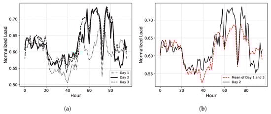
Figure 1.
Examples of the historical average methods. (a) Normalized load for three consecutive days; (b) actual load and historical average.
LI imputes missing values by connecting the values before and after the missing data point with a straight line. Figure 2a compares the imputed values (red dots) using LI when missing occurs in single time slots with the actual values (black line). In cases of a single missing data point, LI is highly effective, as the discrepancies between the actual and imputed values are minimal. However, when consecutive missing occurs over an extended period, the performance of LI significantly deteriorates, as evidenced in Figure 2b. Here, the difference between the values imputed by LI (red line) and the actual values (black line) is substantial, highlighting the inefficiency of LI in dealing with consecutive missing data points. In reality, consecutive missing scenarios occur as frequently as single missing scenarios, necessitating solutions for this specific scenario as well []. Therefore, in the subsequent sections, we focus on autoencoder-based missing imputation techniques, particularly for consecutive missing scenarios.
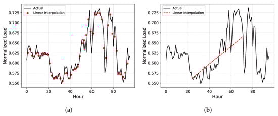
Figure 2.
Examples of the linear interpolation methods. (a) Single missing data point; (b) consecutive missing data points.
3.1. Denoising Autoencoder (DAE)
An autoencoder (AE) is an unsupervised learning task based on the artificial neural network, which consists of a nonlinear encoding function f and a nonlinear decoding function g. In the training phase, we have m DLP data with n time slots. For example, when we have yearly DLP data with 15 min intervals, there are 365 DLP data points with 96 time slots. The DLP data for each date d can be represented by a vector . For a given input vector , f encodes it into a low-dimensional latent feature vector , and g decodes it to the reconstruction vector . This process enables it to learn a feature vector containing essential information from the input data. Even when the input contains a small number of missing values, the feature vectors extracted by the autoencoder can be insensitive to the presence of missing values, making AE widely used in missing imputation tasks [].
Unlike traditional AEs that use the original as the input, denoising autoencoders (DAEs) use a partially corrupted input, denoted as and aim to reconstruct the original . Consequently, DAEs can robustly learn feature vectors, even in the presence of partially corrupted values. In the context of missing imputation, a partially corrupted input refers to artificially introducing missing values into the input DLP data []. Since we specifically focus on handling consecutive missing values, we randomly select a contiguous sequence of U values from a total of n values ranging from to and replace these consecutive U values with zero values, which form the partially corrupted input vector . Here, U represents the missing duration. Therefore, by learning to output the original from the input containing missing values, DAEs can learn the missing imputation process itself. The overall framework of the DAE-based missing imputation is shown in Figure 3. During the training process, fully observable DLP data without any missing values are required. As depicted in Figure 3a, data with randomly generated consecutive missing data points are used as the input, while the original data serve as the output. As illustrated in Figure 3b, the DAE is trained to restore consecutive missing values.
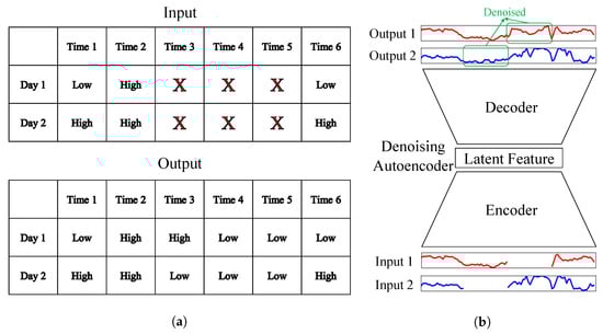
Figure 3.
Illustration of the DAE. (a) Inputs and outputs of the DAE; (b) DAE architectures.
The parameters of the DAE include encoding weight matrices, decoding weight matrices, encoding bias vectors, and decoding bias vectors. During the encoding phase, the feature vectors are extracted as follows:
where and represent the encoding weight matrix and encoding bias vector in the l-th layer, respectively. Here, denotes the nonlinear activation function, and signifies the encoding hidden vector in the l-th layer for a given date d. For , corresponds to the partially corrupted input vector . When the number of hidden layers in the encoder is L, the final output represents the latent feature vectors for date d. Similarly, in the decoding phase, the output vectors are reconstructed as follows:
where and represent the decoding weight matrix and the decoding bias vector in the l-th layer, respectively, and denotes the decoding hidden vector in the l-th layer for date d. For , corresponds to the latent feature vector , and the final output corresponds to the reconstructed output vector . Finally, the total objective function to minimize is formulated as follows:
where is the i-th element of the output vector . Note that the reconstructed value is learned and used as the original input , not the partially corrupted input .
3.2. Masked Autoencoder (MAE)
DAEs have demonstrated to perform effectively in missing imputation, but during the learning process, fully observable DLP data must be utilized as the output. However, in constrained environments with a high missing rate, most DLP data are likely to be partially observable data containing missing values. Applying the DAE directly to this type of data might result in already-existing missing values being learned as zero values during the reconstruction process. While this might not be a significant issue when the missing rate is low, in cases of high missing rates, the zero value reconstruction process can severely degrade the missing imputation performance.
Masked autoencoders (MAEs) can address these issues []. Unlike the assumption in DAE-based missing imputation, the input vector can be a partially observed vector. In other words, missing values filled with zero should not contribute to the reconstruction phase to prevent the network from learning the reconstruction of missing values. Therefore, we define the new error term to consider only the contribution of the observed values, as follows:
where is the set of observed values for day d, and is an indicator function that equals 1 if and 0 otherwise. This loss is called masked reconstruction loss, since missing values are masked in the reconstruction phase.
The reason why missing imputation is possible, even when restoring only observed values, is that it allows similar DLP data to be found during the reconstruction process. This process is illustrated in Figure 4a, where the observed parts of Day 2 and Day 3 are identified as similar, and the similarity is also noticed between Day 3 and Day 4. Consequently, Days 2, 3, and 4 are considered to be similar, and the missing parts can be imputed based on values from dates with similar patterns to the current date. As shown in Figure 4b, MAEs learn to reconstruct only the observed values, ignoring the missing parts during the restoration process. Hence, even with a high missing rate, the performance degradation might not be as significant as in the case of DAEs. This concept aligns with the principles of collaborative filtering in recommendation systems, where predicting a user’s preference for a specific item is based on ratings from similar users to that user [,].
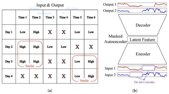
Figure 4.
Illustration of the MAE. (a) Inputs and outputs of the MAE; (b) MAE architectures.
3.3. Proposed Denoising Masked Autoencoder (DMAE)
The MAE has been demonstrated to perform effectively, even in constrained environments with high missing rates. However, the missing imputation process heavily relies on values from dates with similar energy consumption patterns to the current date. This implies that the missing imputation performance can significantly deteriorate when there are few dates with similar energy consumption patterns. Moreover, when the missing rate is exceptionally high, finding dates with similar patterns becomes even more challenging, leading to a drastic degradation in the MAE’s performance. Consequently, there is a need for a technique that combines the DAE’s capability to learn the missing imputation process itself with the MAE’s adaptability to constrained environments with high missing rates.
The proposed denoising masked autoencoder (DMAE)-based missing imputation technique combines the strengths of the DAE and the MAE. Unlike the DAE, it does not require fully observable DLP data; it can be applied even when most DLP data are partially observable due to missing values. In the proposed DMAE method, additional missing values are generated in addition to the pre-existing missing values. In the input DLP data, there are two types of missing values: the ones that already existed and the ones generated additionally. The output DLP data contain only the pre-existing missing values. As in the MAE, the pre-existing missing values are imputed based on values from other dates with similar energy consumption patterns, without being involved in the reconstruction process. The additionally generated missing values are learned through the restoration process, which is similar to the DAE.
The proposed DMAE method is particularly effective for imputing missing values for DLP data with long missing durations using the DLP data with short missing durations. By introducing additional missing values before and after the existing consecutive missing values in DLP data with short missing durations, longer missing durations can be created. Training the model to restore these missing values in the missing generated DLP data allows the model to handle cases with longer missing durations in the test data. Figure 5 illustrates the overall framework of the proposed DMAE. In Figure 5a, the original DLP data with pre-existing missing values serve as the output, while DLP data with additional missing values created before and after the pre-existing missing values are used as the input. As shown in Figure 5b, the previously existing missing values are not engaged in the restoration process, whereas the additionally generated missing values are learned and restored. The total objective function to minimize in the proposed DMAE is formulated as follows:
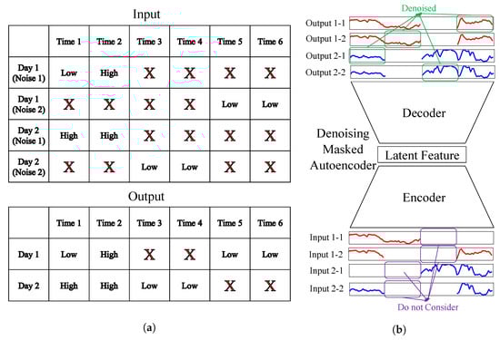
Figure 5.
Illustration of the proposed DMAE. (a) Inputs and outputs of the proposed DMAE; (b) proposed DMAE architectures.
There are differences between Equation (3) and our approach in that we utilized the error term to restore only the observed values. Additionally, our method diverges from Equation (4) as we employed the partially corrupted input instead of the original input . Algorithm 1 summarizes the training process of the proposed DMAE method.
| Algorithm 1 Proposed DMAE-based missing imputation algorithm |
|
The principle driving the enhanced performance of the DMAE over the DAE and MAE can be articulated mathematically. When the value of day d with time slot i is missing, the DAE process inadvertently imposes in Equation (3) due to the absence of masking. Consequently, it trains the model to consistently restore existing missing values as zeros, as is trained to be close to zero, representing an inaccurate missing imputation approach. In contrast, the DMAE addresses this issue by incorporating a masking step for the existing missing values. Since , is set to zero in Equation (5) and is not trained to be close to zero, the flawed restoration training encountered by the DAE is avoided. Consequently, the DMAE achieves a more accurate imputation of missing values compared to the DAE.
In the MAE, the latent vectors are formed based on the similarity of patterns in the data. However, the MAE lacks a denoising process, resulting in an insufficient evaluation and enhancement mechanism for the imputation performance of missing values. As can be seen in Equation (4), the objective function only evaluates the reconstruction accuracy by only reducing the distance from the reconstructed data and observed data . The DMAE, by integrating both a similarity confirmation from MAE and a denoising process, evaluates and improves the imputation performance of the missing values. Equation (5) reduces the distance from the reconstructed data from additional missings and the original observed data . This dual approach enables the DMAE to outperform the MAE in terms of the imputation accuracy.
4. Performance Evaluation
4.1. Experimental Setup
4.1.1. Data Description
We use three electric load datasets for 1 January 2012–31 December 2012 from the USA, which are available on the EnerNoc commercial building dataset []. The first dataset (dataset 14) contains electric load data from the building with business services in Los Angeles, the second dataset (dataset 366) contains electric load data from the building with grocery market in New York, and the third dataset (dataset 716) contains electric load data from the manufacturing building in Chicago. These three selected datasets were chosen to minimize the presence of duplicate values or anomalies, ensuring a more efficient performance evaluation. We preprocessed three electric load datasets to have 15 min granularity, which made the input data size 96. We used min-max normalization to the dataset to improve the model training robustness. Table 1 describes the three datasets.

Table 1.
Data descriptions for the electric load datasets.
As shown in Figure 6, the data were split into a training set, validation set, and test sets. Initially, the total dataset spanning 366 days was grouped into sets of six days each. The first four days of each group were used as training data, the fifth day was used as validation data, and the sixth day was used as test data. This division was designed to reflect situations where missing values occur intermittently throughout the dates []. We defined a target missing duration, denoted as U, and introduced random consecutive missing values of length U into the validation and test datasets. To simulate a scenario where there are missing values in the training data, we also created consecutive missing values of length in the training dataset. This was conducted to assess the performance of missing imputation for long missing durations when training on data with short missing durations.
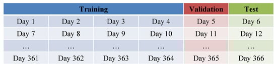
Figure 6.
Dataset Splitting (Training/Validation/Test).
4.1.2. Baseline Model
HA, LI, DAE, and MAE were used for the baseline models. For the HA, we computed the average values from the day-ahead and day-behind data for the missing time slots. Also, as mentioned above, we imputed missing values in the LI model by connecting the values before and after the missing data point with a straight line. In the DAE model, fully observable DLP data should be utilized as the output during the training process. However, we assumed a constrained environment where the training data consist of partially observable DLP data containing missing values. To apply the DAE model in this context, we treated all missing values as zero values to create a situation akin to fully observable DLP data. The MAE model was trained in such a way that missing values did not engage with the reconstruction loss.
4.1.3. Evaluation Metrics
In order to evaluate the performance of each missing imputation scheme, two performance metrics were used, the normalized root mean square error (NRMSE) and the normalized mean absolute error (NMAE), which are given by
where is a set of missing values from the validation dataset or test dataset. When is from a validation dataset, these metrics are used for hyperparameter selection and early stopping, and when is from a test dataset, these metrics are used for performance evaluation.
4.1.4. Hyperparameter Selection
All hyperparameters are summarized in Table 2. To determine the hyperparameters for each model, we observed the normalized root mean square error (NRMSE) over a validation set. The proposed autoencoder consists of two hidden layers () with the input neurons set to 96 (15 min intervals), the hidden neurons to 64, and the latent features to 32. Training additional layers incurs extra training time with little improvement in the validation set performance. All activation functions are sigmoid functions, except for the last one in the decoder network, which does not use an activation function. The network’s learning rate is 0.0001, and a dropout rate of 0.1 is applied to prevent overfitting [,]. All networks are trained using the Adam optimizer [], and our framework is implemented using PyTorch [] with Google Colab GPU.
Table 2.
Hyperparameters.
4.2. Results
Table 3 illustrates the performance of missing imputation for missing durations U of 12, 24, 36, and 48 days, while Figure 7 represents the missing imputation error as a cumulative distribution function (CDF) for dataset 14. First, for the case of , LI exhibited the best performance. This suggests that, in situations with high missing ratios in constrained environments, applying LI for short missing durations is more efficient than other AI-based algorithms. However, for U of more than 24, the performance of the proposed DMAE is the best. Moreover, as U increases, the performance gap of the proposed DMAE with other models becomes more pronounced. HA did not show big performance differences based on the length of U. In contrast, LI, the DAE, and the MAE exceeded an NRMSE of 10 for U values of 36, 24, and 48, respectively. This indicates that these models are highly vulnerable to longer missing durations, leading to a significant degradation in the performance. However, DMAE, our proposed approach, exhibits a much smaller degradation in performance compared to other models for long missing durations. This showcases its robustness against longer missing durations, demonstrating significantly less vulnerability than other models.
Table 3.
Experiment results for dataset 14.
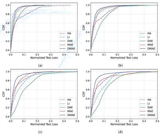
Figure 7.
CDF of the missing imputation error of dataset 14. (a) . (b) . (c) . (d) .
Table 4 and Figure 8 present the results for dataset 366. In the case of dataset 14, LI exhibited a superior performance to the HA at both and . However, in dataset 366, LI and the HA showed similar performances at , and from onwards, the HA overwhelmingly outperformed LI. This suggests that this dataset represents a scenario where the HA is more suitable than LI, possibly due to the DLP data displaying similar values at the same time slots. The DAE and the MAE experienced drastic performance deteriorations, exceeding an NRMSE of 10 for U values of 24 and 48, respectively. In contrast, DMAE not only showed no significant decline in performance but also demonstrated the best performance in terms of missing imputation for all cases of U. This implies that, even in datasets where HA performs well, DMAE can surpass HA’s performance, especially in scenarios with very long missing durations.
Table 4.
Experimental results for dataset 366.
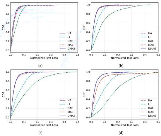
Figure 8.
CDF of the missing imputation error of dataset 366. (a) . (b) . (c) . (d) .
Table 5 and Figure 9 present the results for dataset 716. In contrast to the case of dataset 14, where LI performed the best only for , LI demonstrated a superior performance, not only for but also for for dataset 716. This discrepancy is because of the prominent linearity observed in dataset 716 compared to dataset 14, which indicates that the criterion for the missing duration U for applying LI instead of AI-based algorithms in missing imputation varies across datasets. The DAE and the MAE experienced drastic deteriorations in performance again, exceeding an NRMSE of 10 for U values of 24 and 48, respectively. Neither LI nor DMAE exhibited sharp declines in performance; however, for U of more than 36, DMAE outperformed LI in terms of missing imputation. This suggests that, even in datasets with significant linearity, DMAE can surpass LI’s performance, especially in scenarios with very large missing durations.
Table 5.
Experimental results for dataset 716.
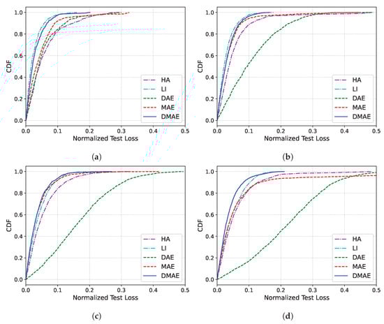
Figure 9.
CDF of the missing imputation error for dataset 716. (a) . (b) . (c) . (d) .
To visualize the imputation result, the examples of the actual electric load curves and missing imputation results for datasets 14, 366, and 716 are given in Figure 10, Figure 11 and Figure 12, respectively, for the cases of and . It has been observed that HA, except for in special cases like dataset 366, fails to properly follow the actual load curve, indicating that it is generally not suitable from an end customer perspective. Furthermore, it is evident that LI’s performance is subpar when linearity is absent, particularly in dataset 14, where the linearity is even lower. The DAE and the MAE both experience significant performance deteriorations as U increases. In contrast, the DMAE consistently outperforms other methods, closely tracking the actual load curve, regardless of the missing duration.
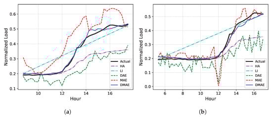
Figure 10.
The examples of the actual electric load curve and missing imputation results for dataset 14. (a) . (b) .
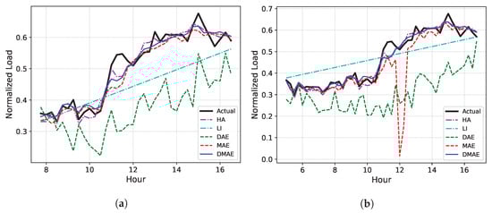
Figure 11.
The examples of the actual electric load curve and missing imputation results for dataset 366. (a) . (b) .
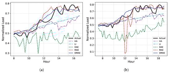
Figure 12.
The examples of the actual electric load curve and missing imputation results for dataset 716. (a) . (b) .
We utilized a very basic autoencoder structure in our study. Considering the advancements in generative model technologies, one might question whether employing more advanced autoencoder techniques, such as the variational autoencoder (VAE) or Wasserstein autoencoder (WAE), would be more efficient. In fact, these technologies are widely used for missing imputation in various fields and differ from the basic autoencoder in terms of forcing the feature space as a Gaussian distribution. However, as observed in previous research [], when trained with a small amount of data, less than one year in length, the basic structure of the autoencoder outperforms the VAE or WAE. Figure 13, Figure 14 and Figure 15 depict the probability density function (PDF) of the first components of the feature vectors obtained from the training data after training DMAE. As is evident in the figures, the shape closely resembles a zero-mean Gaussian distribution. If the feature space is naturally shaped similarly to a Gaussian distribution, forcing it into a Gaussian distribution might distract the focus of the training from missing imputation, potentially degrading the learning performance. Hence, when training with a limited amount of data, the basic autoencoder demonstrates a superior performance.
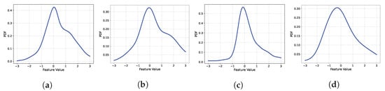
Figure 13.
PDF of the first elements of the feature vectors of DMAE for dataset 14. (a) . (b) . (c) . (d) .
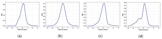
Figure 14.
PDF of the first elements of the feature vectors of DMAE for dataset 366. (a) . (b) . (c) . (d) .
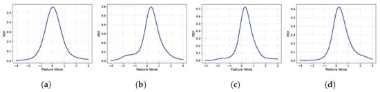
Figure 15.
PDF of the first elements of the feature vectors of DMAE for dataset 716. (a) . (b) . (c) . (d) .
5. Conclusions
In this paper, we proposed a novel consecutive missing imputation framework called the DMAE for DLP data. The proposed DMAE leverages both the ability to learn missing imputation processes from the DAE and the advantage of the MAE of being applicable in constrained environments with high missing data rates. To achieve this, we introduce additional missing values before and after the existing consecutive missing data. The newly generated missing values are then trained for restoration, while the original missing values are not engaged in the loss function. Extensive simulations with three electric load datasets showed that the proposed DMAE outperforms the other forecasting models based on the HA, LI, the DAE, and the MAE in terms of the NRMSE and NMAE. Also, the proposed DMAE shows the lowest performance degradation when the missing duration increases.
The proposed study leveraged the strengths of the DAE and the MAE to enhance the performance in environments with high missing ratios. However, the performance evaluation has, so far, been conducted only in situations where there is a single consecutive missing block for each DLP dataset. Therefore, there is a need for additional research to evaluate the performance across various missing patterns. For instance, scenarios may involve a mix of single and consecutive missing blocks, or there might be multiple consecutive missing blocks within a single DLP dataset. In such cases, it is necessary to investigate the most efficient way to generate missing data for training the DMAE, considering the different patterns of missing data that may occur. We expect that the DMAE can be further extended by being combined with other algorithms. For example, the combination of the DMAE and the transformer could capture the temporal features of the DLP data much better. Also, the DMAE and graph neural networks can be combined to find similar energy consumption patterns much more easily from other dates or other electric load sites.
Author Contributions
Conceptualization, J.J., T.-Y.K. and W.-K.P.; methodology, J.J.; software, J.J.; validation, J.J., T.-Y.K. and W.-K.P.; writing—original draft preparation, J.J.; writing—review and editing, J.J.; visualization, J.J.; supervision, W.-K.P.; project administration, T.-Y.K. All authors have read and agreed to the published version of the manuscript.
Funding
This work was supported by the Korea Institute of Energy Technology Evaluation and Planning (KETEP) and the Ministry of Trade, industry & Energy (MOTIE) of Korea (No. 2021202090028C).
Data Availability Statement
The data presented in this study are openly available [].
Conflicts of Interest
The authors declare no conflict of interest.
Abbreviations
The following abbreviations are used in this manuscript:
| DLP | Daily load profile |
| HA | Historical average |
| LI | Linear interpolation |
| DAE | Denoising autoencoder |
| MAE | Masked autoencoder |
| DMAE | Denoising masked autoencoder |
| Proability density function | |
| CDF | Cumulative distribution function |
References
- Massaoudi, M.; Abu-Rub, H.; Refaat, S.S.; Chihi, I.; Oueslati, F.S. Deep learning in smart grid technology: A review of recent advancements and future prospects. IEEE Access 2021, 9, 54558–54578. [Google Scholar] [CrossRef]
- Emmanuel, T.; Maupong, T.; Mpoeleng, D.; Semong, T.; Mphago, B.; Tabona, O. A survey on missing data in machine learning. J. Big Data 2021, 8, 1–37. [Google Scholar] [CrossRef]
- Peppanen, J.; Zhang, X.; Grijalva, S.; Reno, M.J. Handling bad or missing smart meter data through advanced data imputation. In Proceedings of the 2016 IEEE Power & Energy Society Innovative Smart Grid Technologies Conference (ISGT), Minneapolis, MN, USA, 6–9 September 2016; pp. 1–5. [Google Scholar]
- Ryu, S.; Choi, H.; Lee, H.; Kim, H. Convolutional autoencoder based feature extraction and clustering for customer load analysis. IEEE Trans. Power Syst. 2019, 35, 1048–1060. [Google Scholar] [CrossRef]
- Noor, N.M.; Al Bakri Abdullah, M.M.; Yahaya, A.S.; Ramli, N.A. Comparison of linear interpolation method and mean method to replace the missing values in environmental data set. Mater. Sci. Forum 2015, 803, 278–281. [Google Scholar] [CrossRef]
- Zhang, J.; Yin, P. Multivariate time series missing data imputation using recurrent denoising autoencoder. In Proceedings of the 2019 IEEE International Conference on Bioinformatics and Biomedicine (BIBM), San Diego, CA, USA, 18–21 November 2019; pp. 760–764. [Google Scholar]
- Ryu, S.; Kim, M.; Kim, H. Denoising autoencoder-based missing value imputation for smart meters. IEEE Access 2020, 8, 40656–40666. [Google Scholar] [CrossRef]
- De Wit, T.D. A method for filling gaps in solar irradiance and solar proxy data. Astron. Astrophys. 2011, 533, A29. [Google Scholar] [CrossRef]
- Luo, Y.; Cai, X.; Zhang, Y.; Xu, J.; Xiaojie, Y. Multivariate time series imputation with generative adversarial networks. Adv. Neural Inf. Process. Syst. 2018, 31, 1–12. [Google Scholar]
- De Paz-Centeno, I.; García-Ordás, M.T.; García-Olalla, Ó.; Alaiz-Moretón, H. Imputation of missing measurements in PV production data within constrained environments. Expert Syst. Appl. 2023, 217, 119510. [Google Scholar] [CrossRef]
- Sedhain, S.; Menon, A.K.; Sanner, S.; Xie, L. Autorec: Autoencoders meet collaborative filtering. In Proceedings of the 24th International Conference on World Wide Web, Florence, Italy, 18–22 May 2015; pp. 111–112. [Google Scholar]
- Yoon, J.; Jordon, J.; Schaar, M. Gain: Missing data imputation using generative adversarial nets. In Proceedings of the International Conference on Machine Learning, PMLR, Stockholm, Sweden, 10–15 July 2018; pp. 5689–5698. [Google Scholar]
- Zhang, W.; Luo, Y.; Zhang, Y.; Srinivasan, D. SolarGAN: Multivariate solar data imputation using generative adversarial network. IEEE Trans. Sustain. Energy 2020, 12, 743–746. [Google Scholar] [CrossRef]
- Hwang, J.; Suh, D. CC-GAIN: Clustering and Classification-Based Generative Adversarial Imputation Network for Missing Electricity Consumption Data Imputation; SSRN 4617547; Elsevier: Amsterdam, The Netherlands, 2023. [Google Scholar]
- Hu, X.; Zhan, Z.; Ma, D.; Zhang, S. Spatiotemporal Generative Adversarial Imputation Networks: An Approach to Address Missing Data for Wind Turbines. IEEE Trans. Instrum. Meas. 2023, 72, 3530508. [Google Scholar] [CrossRef]
- Zhao, L.; Wang, Z.; Chen, T.; Lv, S.; Yuan, C.; Shen, X.; Liu, Y. Missing interpolation model for wind power data based on the improved CEEMDAN method and generative adversarial interpolation network. Glob. Energy Interconnect. 2023, 6, 517–529. [Google Scholar] [CrossRef]
- Li, Y.; Song, L.; Hu, Y.; Lee, H.; Wu, D.; Rehm, P.; Lu, N. Load Profile Inpainting for Missing Load Data Restoration and Baseline Estimation. IEEE Trans. Smart Grid 2023. [Google Scholar] [CrossRef]
- Mescheder, L.; Nowozin, S.; Geiger, A. The numerics of gans. Adv. Neural Inf. Process. Syst. 2017, 30, 1–11. [Google Scholar]
- Goodfellow, I.; Bengio, Y.; Courville, A. Deep Learning; MIT Press: Cambridge, MA, USA, 2016. [Google Scholar]
- Raghuvamsi, Y.; Teeparthi, K.; Kosana, V. Denoising autoencoder based topology identification in distribution systems with missing measurements. Int. J. Electr. Power Energy Syst. 2023, 154, 109464. [Google Scholar] [CrossRef]
- Kuppannagari, S.R.; Fu, Y.; Chueng, C.M.; Prasanna, V.K. Spatio-temporal missing data imputation for smart power grids. In Proceedings of the 12th ACM International Conference on Future Energy Systems, Virtual, 28 June–2 July 2021; pp. 458–465. [Google Scholar]
- Marco, R.; Syed Ahmad, S.S.; Ahmad, S. Missing Data Imputation Via Stacked Denoising Autoencoder Combined with Dropout Regularization Based Small Dataset in Software Effort Estimation. Int. J. Intell. Eng. Systems 2022, 15, 253–267. [Google Scholar]
- Park, K.; Jeong, J.; Kim, D.; Kim, H. Missing-insensitive short-term load forecasting leveraging autoencoder and LSTM. IEEE Access 2020, 8, 206039–206048. [Google Scholar] [CrossRef]
- Park, H.; Jeong, J.; Oh, K.W.; Kim, H. Autoencoder-Based Recommender System Exploiting Natural Noise Removal. IEEE Access 2023, 11, 30609–30618. [Google Scholar] [CrossRef]
- Wang, Y.; Xu, H.; Xu, Z.; Gao, J.; Wu, Y.; Zhang, Z. Multivariate Time Series Imputation Based on Masked Autoencoding with Transformer. In Proceedings of the 2022 IEEE 24th International Conference on High Performance Computing & Communications; 8th International Conference on Data Science & Systems; 20th Int Conf on Smart City; 8th International Conference on Dependability in Sensor, Cloud & Big Data Systems & Application (HPCC/DSS/SmartCity/DependSys), Hainan, China, 18–20 December 2022; pp. 2110–2117. [Google Scholar]
- EnerNOC. EnerNOC Commerical Building Dataset. Available online: https://open-enernoc-data.s3.amazonaws.com/anon/index.html (accessed on 23 October 2023).
- Jeong, D.; Park, C.; Ko, Y.M. Missing data imputation using mixture factor analysis for building electric load data. Appl. Energy 2021, 304, 117655. [Google Scholar] [CrossRef]
- Srivastava, N.; Hinton, G.; Krizhevsky, A.; Sutskever, I.; Salakhutdinov, R. Dropout: A simple way to prevent neural networks from overfitting. J. Mach. Learn. Res. 2014, 15, 1929–1958. [Google Scholar]
- Steck, H. Autoencoders that don’t overfit towards the identity. Adv. Neural Inf. Process. Syst. 2020, 33, 19598–19608. [Google Scholar]
- Kingma, D.P.; Ba, J. Adam: A method for stochastic optimization. arXiv 2014, arXiv:1412.6980. [Google Scholar]
- Paszke, A.; Gross, S.; Massa, F.; Lerer, A.; Bradbury, J.; Chanan, G.; Killeen, T.; Lin, Z.; Gimelshein, N.; Antiga, L.; et al. Pytorch: An imperative style, high-performance deep learning library. Adv. Neural Inf. Process. Syst. 2019, 32, 1–12. [Google Scholar]
Disclaimer/Publisher’s Note: The statements, opinions and data contained in all publications are solely those of the individual author(s) and contributor(s) and not of MDPI and/or the editor(s). MDPI and/or the editor(s) disclaim responsibility for any injury to people or property resulting from any ideas, methods, instructions or products referred to in the content. |
© 2023 by the authors. Licensee MDPI, Basel, Switzerland. This article is an open access article distributed under the terms and conditions of the Creative Commons Attribution (CC BY) license (https://creativecommons.org/licenses/by/4.0/).