Maximum Power Point Tracking Control of Offshore Hydraulic Wind Turbine Based on Radial Basis Function Neural Network

Abstract

A maximum power point tracking control strategy for an affine nonlinear constant displacement pump-variable hydraulic motor actuation system with parameter uncertainty, used within an offshore hydraulic wind turbine, is studied in this paper. First, we used the feedback linearization method to solve the affine nonlinear problem in the system. However, offshore hydraulic wind turbines have strong parameter uncertainty characteristics. This conflict was resolved through the further application of RBF neural network adaptive control theory. So, we combined feedback linearization with RBF adaptive control as the control theory, and then two control laws were compared by setting the pump rate and rating as outputs, respectively. It is shown by the MATLABR2016a/Simulink emulation results that power control is smoother than speed and friendlier for electric networks. It is also shown by the emulation results, in terms of the undulatory wind speed condition, that the feedback linearization–RBF neural network adaptive control strategy has perfect robustness. According to the simulation results, the feedback linearization–RBF neural network adaptive control strategy adopts the RBF neural network to approach complex nonlinear models and solve the parameter uncertainty problem. This control law also avoids the use of feedback linearization control alone, which can result in the system becoming out of control.

1. Introduction

During the 2021–2030 period, the use of renewable power must be expanded by 12% to achieve net zero levels [1], according to the International Energy Agency. As an important renewable energy, wind power generation should assume a greater share of the market because wind turbines emit far less greenhouse gases than coal-fired power plants in the same cycle [2]. Compared with onshore wind turbines, offshore wind turbines have the remarkable advantage of a large installed capacity [3], which meets certain economic development goals. According to the “Global Wind Energy Report 2022” published by the Global Wind Energy Council, the power produced worldwide by offshore wind farms was 21.1 GW in 2021, which is more than three times that produced in 2020. As a result, increasing attention has been paid to offshore wind generation by major economic powers. In coastal areas of China, the quality of offshore wind energy is better than that of onshore wind energy [4]. Considering the population, economy, and other factors, there are good prospects for the development of Chinese offshore wind generation.

At present, most wind farms deploy traditional wind turbines: direct drive turbines (DDTs) and gear drive turbines (GDTs) [5]. The electric motors used in DDTs are more expensive and, due to the permanent neodymium (Nd) magnets incorporated in these electric motors, metal tools cannot be used to maintain them. The problem with GDTs is their high cost of installation and maintenance of the gear drive unit [6]. Compared with DDTs, GDTs are more commonly used in offshore wind farms. Due to the huge volume and complex structure of the variable speed gearbox, the expenses of those projects, their usage and maintenance, the structure’s design, and the logistics of mobilizing maintenance personnel with equipment to an offshore location account for the majority of the costs of offshore wind farms [7]. The hydraulic transmission system (HTS) used in hydraulic wind turbines (HWTs) has the advantages of high reliability and the flexible arrangement of the hydraulic components through long pipelines. It can be used to reduce the costs of offshore wind turbine installation, operational maintenance, and infrastructure, as well as allowing the levelized cost of energy (LCOE) to reduce as the number of wind turbines installed increases [8].

The maximum power point tracking (MPPT) control strategy is to control wind turbines to capture the maximum amount of wind power under the operating wind speed, after connection to the power grid, to improve efficiency and reduce operating costs. This strategy is conducted for all types of wind turbines. Bastiani et al. [9] combined adaptive MPPT control with a self-adaptable virtual synchro generator to expand the inertial response of type 4 wind turbines. Li et al. [10] applied a model predictive control (MPC) strategy to track the maximum power point. Lin et al. [11] designed a nonlinear optimum rotor speed tracker to realize MPPT control. By comparing the MPPT control strategies with controlling generator torque and pitch angle, it can be concluded that controlling generator torque shows a better performance [12,13]. Although the abovementioned MPPT methods are aimed at DDTs or GDTs, they still provide ideas for HWT control strategies.

MPPT control strategies for HWT have recently been studied, and these strategies can be realized through tip speed ratio [14]. Taking the hydraulic pump speed as the output, the active disturbance rejection control (ADRC) method was introduced to achieve HWT MPPT control [15]. Nevertheless, the control smoothness needs to be further improved. Based on small-signal linearization and variable gain proportional integral differentiation (PID), Ai et al. [16] controlled HWT output power to realize MPPT. However, this method causes increased system errors because the HTS of offshore HWTs has complex nonlinear characteristics [17]. Farbood et al. [18] used the MPC strategy to solve the MPPT control problem in HWTs; however, this method increases the amount of calculations necessary and the burden on the hardware due to the system’s strong nonlinearity.

The complex nonlinearity of HTS results in higher requirements for the MPPT control strategy. Feedback linearization (FL) comes from differential geometry theory and can deal with affine nonlinear HWT systems through state changes and feedback simply and efficiently [19]. Nonetheless, FL demands a rigorous mathematical model, which means that each parameter should be known exactly. However, the parameters of HTS, e.g., the leakage coefficient $C_t$ and bulk modulus $\beta$, cannot be accurately obtained [20,21]. This is because they change with the state of the hydraulic transmission system (such as pressure or temperature). This parameter uncertainty is greatly affected by the large load of offshore HWTs because this characteristic of offshore HWTs can cause great pressure in the HTS. So, it is difficult to establish an accurate model, such as that required by feedback linearization, in real applications. The empirical values often used in research may cause steady-state errors and may even lead to the system becoming out of control. The adaptive control method was also employed to solve the parameter uncertainty of hydraulic systems [22,23,24,25,26]. However, it cannot solve this problem well for HTSs with complex nonlinearity. Instead, a combination of RBF neural network theory and adaptive control can solve this problem effectively [27,28,29,30].

This paper proposes a feedback linearization–RBF neural network adaptive (FL-RBFA) MPPT control strategy. To resolve affine nonlinearity with parameter uncertainty in MPPT control of offshore HWTs, the FL method was first used to deal with the nonlinearity and eliminate the limitation of small-signal linearization [19]. The HTS of the HWT has the parameter uncertainty characteristics, but the FL method needs an accurate mathematical model. Then, aiming at this conflict, the RBF adaptive control law was used to improve the FL method.

This paper is organized as follows: the HWT mathematical model is established in Section 2. The design of an FL-RBFA MPPT control strategy with hydraulic pump speed as the output is shown in Section 3. To overcome its power control defects, an investigation of the FL-RBFA MPPT control with hydraulic pump power as the output is conducted in Section 4. The simulation results are discussed in Section 5, and the conclusion is given in Section 6.

2. Modeling of Hydraulic Wind Turbine

On the basis of the generator model simplified using aerodynamics, each wind speed received its corresponding optimal hydraulic pump speed. Then, the relationship was derived between maximum wind power capture and optimal hydraulic pump speed under each wind speed condition. After that, a state-space equation model was established. On the basis of the above, the MPPT principle was used to obtain the ideal control law by separately taking the speed and power of the hydraulic pump as the output. The unknown functions and parameters existing in the ideal control rate were approximated by the RBF and adaptive control rate.

2.1. Working Principle of Offshore Hydraulic Wind Turbine

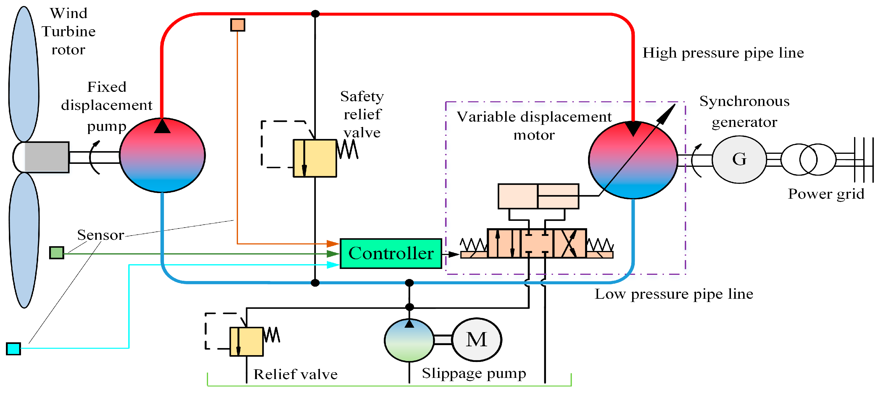
The offshore HWT is shown in Figure 1 in this paper. This turbine mainly comprises a rotor, a quantified pump, a variable motor and a alternator. It does not need an inverter for frequency conversion because of the hydraulic system inherent variable ratio. The hydraulic motor is coaxially connected with generator, and the system is controlled by changing the motor displacement. According to the Chinese National Standards, the wind turbine can be connected to the grid only when the frequency of the generator is 50 ± 0.2 Hz. In other words, the motor speed is 1500 ± 6 r/min. After grid connection, the HWT needs MPPT control to ensure that the HWT can capture enough wind power.

2.2. The Wind Turbine Rotor Model

In

Table 1. Symbols and their meanings.

Symbols	Symbolic Meaning	Symbols	Symbolic Meaning
$\rho$	Air density	$C_t$	Leak coefficient
$R$	Wind turbine radius	$V$	High pressure volume
$v$	Wind speed	$K_m$	Motor maximum displacement
$C_p$	Coefficient of wind energy utilization	$\gamma$	Motor swing angle
$C_{p\max }$	Maximum coefficient of wind energy utilization	$\zeta$	Input of neural network
${\omega }_p$	Pump speed	$h\left(x\right)$	Gaussian function
$\lambda$	Blade tip speed ratio	$W$	Weight of the network
${\lambda }_{opt}$	Optimum blade tip speed ratio	$i$	Number of neural network inputs
$\theta$	Pitch angle	$j$	Hidden layer node of neural network
$B_p$	Pump viscous damping coefficient	$c_{ij}$	Coordinate of the center point of the Gaussian basis function
$J_p$	Pump moment of inertia	$b_j$	Width of the Gaussian basis function
$D_p$	Pump displacement	$\epsilon$	Approximation error of neural network
$p_h$	High pressure	$\varsigma$	Coefficients in Lyapunov function
$\beta$	Oil bulk modulus

, we show symbols and their meanings in the following formula.

The actual wind turbine rotor model is relatively complex. In order to facilitate the research, a simplified mathematical model based on aerodynamic principles [31] was adopted. When wind turbines rotor work under the operating wind speed, the wind power captured is expressed as

$$P_r=\frac{1}{2}\rho \pi R^2{v}^3{C}_p\left(\lambda ,\theta \right)$$

(1)

The wind energy utilization coefficient $C_p$ can be expressed as

$$C_p(\lambda ,\theta )=C_1(\frac{C_2}{{\lambda }_i}-C_3\theta -C_4)e^{-\frac{C_5}{{\lambda }_i}}+C_6\lambda$$

(2)

$$\frac{1}{{\lambda }_i}=\frac{1}{\lambda +0.08\theta }-\frac{0.035}{{\theta }^3+1}$$

(3)

After determining the wind turbine blade shape, the parameters $C_1$, $C_2$, $\cdots$, $C_6$ are known. The model of this research mainly refers to an 850 kW HWT. According to the manual, $C_1=0.5176$, $C_2=116$, $C_3=0.4$, $C_4=5$, $C_5=21$, $C_6=0.003$. In the process of MPPT control, the pitch angle $\theta$ is 0.

The torque generated by the rotor to the HTS can be expressed as

$$T_r=\frac{P_r}{{\omega }_r}$$

(4)

Because of coaxially connecting the rotor with the hydraulic pump, they have the same speed, i.e., ${\omega }_r={\omega }_p$. Thus, the blade tip speed ratio coefficient $\lambda$ can be expressed by

$$\lambda =\frac{R{\omega }_r}{v}=\frac{R{\omega }_p}{v}$$

(5)

From Equation (1), the wind power captured by the wind turbine is determined by the wind energy utilization coefficient $C_p$ when the wind speed is determined. According to Equations (2) and (3), $C_p$ is related to the blade tip speed ratio coefficient $\lambda$. There is a optimal blade tip speed ratio coefficient ${\lambda }_{opt}$ corresponding to the maximum coefficient of wind energy utilization $C_{p\max }$, at which point wind turbines capture the most wind.

By differentiating Equation (2) with $\lambda$, it can be obtained that $C_{p\max }$ is 0.4496, and the corresponding ${\lambda }_{opt}$ is 8.019.

The optimal blade tip speed ratio coefficient ${\lambda }_{opt}$ means that each wind speed corresponds to an optimal hydraulic pump speed.

$${\lambda }_{opt}=\frac{R{\omega }_{opt}}{v}$$

(6)

When the wind speed changes, maximum wind power is captured by the wind turbine by adjusting the hydraulic pump speed ${\omega }_p$ to the optimal speed ${\omega }_{opt}$.

Combining Equations (1) and (6), the relationship between $P_{r\max }$ and ${\omega }_{opt}$ can be expressed as

$$P_{r\max }=\frac{\rho \pi R^5{C}_{p\max }}{2{\lambda }_{opt}^3}{\omega }_{opt}^3=K_{\omega }{\omega }_{opt}^3$$

(7)

where $P_{r\max }$ is the maximum wind power captured by the wind turbine rotor at the current wind speed and ${\omega }_{opt}$ is the optimal hydraulic pump speed.

${\lambda }_{opt}=8.019$ was calculated above using the data of the 850 kW HWT. In this research, the 850 kW HWT was replaced by a 24 kW HWT hardware-in-the-loop experiment platform that is composed of a wind turbine simulation module, a quantitative pump-variable motor-hydraulic transmission system, a control system, and a power generation system. The ${\lambda }_{opt}=22.791$ of the 24 kW HWT hardware-in-the-loop experiment platform comes from the 850 kW HWT through similar calculation [32]. The basic parameters of the two wind turbines are shown in

Table 2. Basic parameters of wind turbines.

Rated Power (kW)	Rotor Radius (m)	Rated Rotor Speed (r/min)	Rated Wind Speed (m/s)
850	22.283	45	13
24	3.74	762	13

.

2.3. Principle of MPPT

The MPPT of offshore HWT can be realized through taking the pump speed Equation (6) and pump power Equation (7) as control targets, respectively, shown in Figure 2 and Figure 3.

In engineering, the number of revolutions per minute ($n$, $\mathrm{r}/\min$) is often used to replace the angular velocity ($\omega$, $\mathrm{rad}/\mathrm{s}$). The relationship between them is $n=\frac{60}{2\pi }\omega$. In the next figures, $n$ will be used instead of $\omega$.

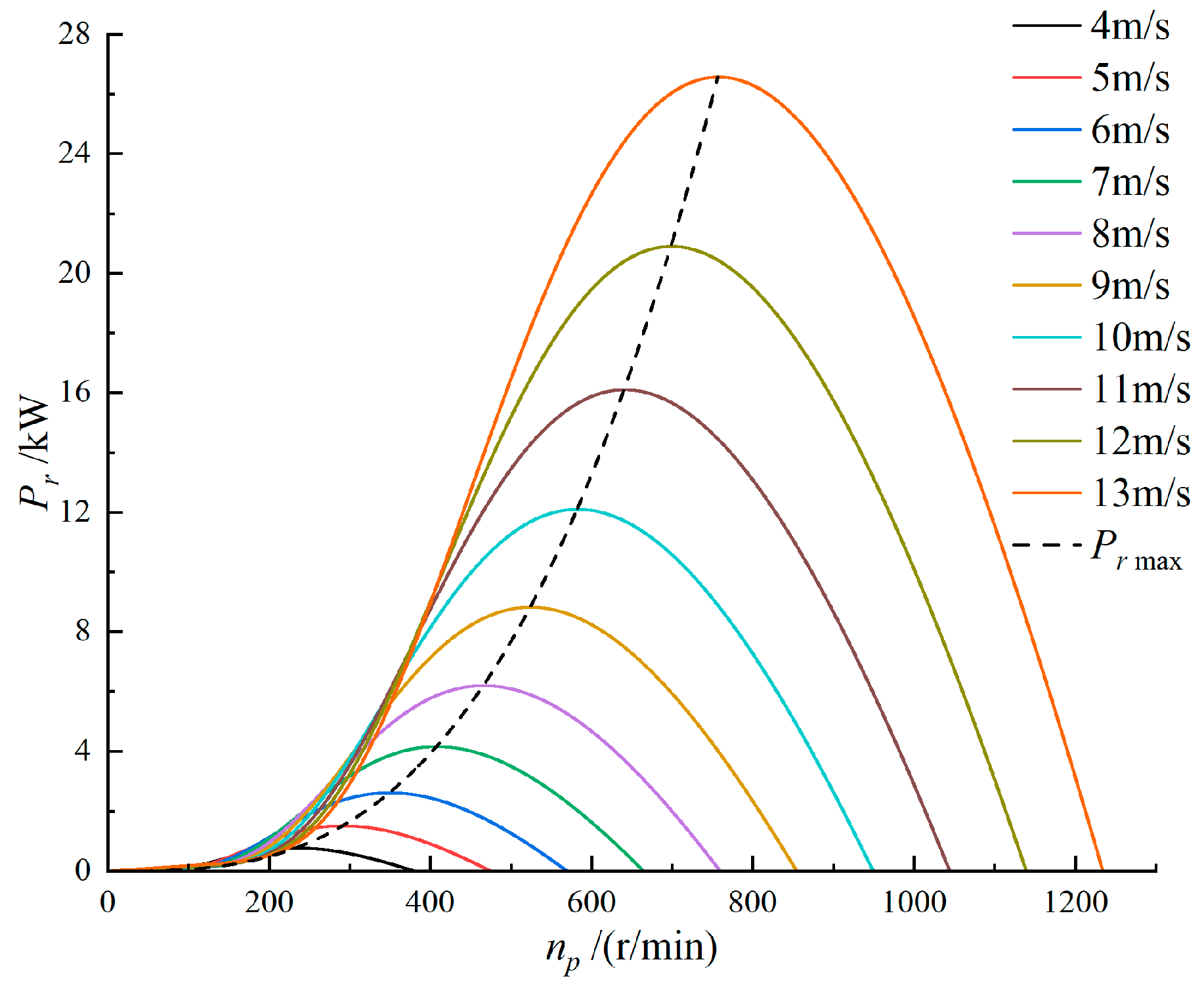
The relationship between captured wind power and hydraulic pump speed (i.e., wind turbine characteristic curve) is shown in Figure 2. The wind turbine characteristic curves were obtained using simultaneous Equations (1)–(6). Each solid curve has a maximum power point, which means that the wind turbine can capture the maximum wind power with this pump speed under the current wind speed. The dotted curve $P_{r\max }$ (maximum power curve) can be obtained by connecting each maximum power point. The best power curve corresponds to Equation (7). The goal of MPPT control of HWT with hydraulic pump speed as output is to control the pump to reach the optimal pump speed under current wind speed.

According to Figure 2 and Equation (7), we also obtain the MPPT control with hydraulic pump power as output. The principle is shown in Figure 3.

The tracking process is expressed as follows:

Assuming wind speed $v_1<v_2<v_3$, C, A, and B are the maximum power points at the three wind speeds, respectively. The initial operating condition of the wind turbine is $v_2$. The wind turbine started at point A, which is the maximum power point at wind speed $v_2$.

When the wind speed increases from $v_2$ to $v_3$, the rotor speed cannot change suddenly, but the rotor capture power changes from $P_A$ (point A) to $P_D$ (point D) shown in Equation (1). At the same time, the wind turbine output power is still $P_A$. Since the rotor capture power is greater than the output power before point B, the rotor accelerates. As the rotor speed increases, the rotor capture power moves along the wind turbine characteristic curve of $v_3$ from point D to the maximum power point B. Additionally, the turbine output power moves along the maximum power curve from point A to point B. The system re-balances at point B.

Analogously, when the wind speed decreases from $v_2$ to $v_1$, the captured power is the $P_E$ corresponding to point E. At this time, the wind turbine output power is still $P_A$. Since the input power is always smaller than the output power before point C, the rotor would decelerate. As the rotor speed reduction, the input power moves from point E to the maximum power point C along the wind turbine characteristic curve of $v_1$. Additionally, the output power moves from A to C along the maximum power curve. The system is re-balanced at point C.

2.4. The HTS Mathematic Model

Ai C et al. showed the specific mathematical expression of each component of HTS in their article [19].

The following assumptions were made to establish the system state space model:

• Low pipeline pressure is a constant;
• The pressure loss in hydraulic pipe lines is ignored;
• The hydraulic pump mechanical efficiency ${\eta }_{mech,p}$ and the hydraulic motor mechanical efficiency ${\eta }_{mech,m}$ are designed as constant 1.

The system state space model can be expressed as [19]

$$\left\{\begin{array}{l}{\dot{\omega }}_p=-\frac{B_p}{J_p}{\omega }_p-\frac{D_p}{J_p}{p}_h+\frac{1}{J_p}{T}_r({\omega }_p,v)\\ {\dot{p}}_h=\frac{D_p\beta }{V}{\omega }_p-\frac{C_t\beta }{V}{p}_h-\frac{K_m\beta {\omega }_m}{V}\gamma \end{array}\right.$$

(8)

It also can be expressed in a different way

$$\left\{\begin{array}{l}{\dot{x}}_1=-\frac{B_p}{J_p}{x}_1-\frac{D_p}{J_p}{x}_2+\frac{1}{J_p}{T}_r(x_1,v)\\ {\dot{x}}_2=\frac{D_p\beta }{V}{x}_1-\frac{C_t\beta }{V}{x}_2-\frac{K_m\beta {\omega }_m}{V}u\end{array}\right.$$

(9)

where $x={[\begin{array}{cc}{x}_1& x_2\end{array}]}^{\mathrm{T}}={[\begin{array}{cc}{\omega }_p& p_h\end{array}]}^{\mathrm{T}}$, $u=\gamma$.

The system conforms to the affine nonlinear standard form $\dot{x}=f(x)+g(x)u$, where

$$f(x)=\left[\begin{array}{c}\begin{array}{ccc}-\frac{B_p}{J_p}& -\frac{D_p}{J_p}& \frac{1}{J_p}\end{array}\\ \begin{array}{ccc}\frac{D_p\beta }{V}& -\frac{C_t\beta }{V}& 0\end{array}\end{array}\right]\left[\begin{array}{c}{x}_1\\ x_2\\ T_r(x_1,v)\end{array}\right]$$

(10)

$$g(x)=\left[\begin{array}{c}0\\ -\frac{K_m{\omega }_{md}\beta }{V}\end{array}\right]$$

(11)

In this research, we used FL theory to deal with the affine nonlinear system state space model.

3. Design of Mppt Control Law with Hydraulic Pump Speed as Output

In order to apply feedback linearization, the controllability and atropodotation conditions should first be examined. The controllability matrix can be expressed as

$$\left[\begin{array}{cc}g& a{d}_{f}g\end{array}\right]=\left[\begin{array}{cc}0& -\frac{K_m{\omega }_{md}\beta D_p}{J_{p}V}\\ -\frac{K_m{\omega }_{md}\beta }{V}& -\frac{K_m{\omega }_{md}\beta C_t}{V^2}\end{array}\right]$$

(12)

Considering the physical meaning of each symbol, the matrix is full rank. Therefore, the system is controllable. Because of the constant vector fields $\left[\begin{array}{cc}g& a{d}_{f}g\end{array}\right]$, they form an involutive set.

The relative order of the system can be obtained next.

Taking the pump speed as the control output, the output is

$$y=h(x)=x_1$$

(13)

The system relative order is deduced as follows

$$\left\{\begin{array}{l}{L}_g{L}_f^{0}h(x)=0\\ L_g{L}_f^{1}h(x)=\frac{D_{p}K\beta }{J_{p}V}\end{array}\right.$$

(14)

It can be obtained from Equation (14) that the relative order of the control system with pump speed as output is $r=2$. The order of the HTS is also $n=2$ from Equation (9). Therefore, the control system meets requirements of input-state linearization when taking the hydraulic pump speed as the output.

To realize feedback linearization, the system state coordinates can be altered as

$$\left\{\begin{array}{l}{\dot{z}}_1=z_2\\ {\dot{z}}_2=L_f^{2}h(x)+L_g{L}_{f}h(x)u\end{array}\right.$$

(15)

The first component $z_1$ of the new state $z={\left[\begin{array}{cc}{z}_1& z_2\end{array}\right]}^{\mathrm{T}}$ can be expressed as

$$z_1=x_1$$

(16)

Therefore, the system state coordinates can be expressed as

$$\left\{\begin{array}{l}{\dot{z}}_1=z_2\\ {\dot{z}}_2=\left[\left(-\frac{D_p^2\beta }{J_{p}V}-\frac{C_t{B}_p\beta }{J_{p}V}\right)z_1+\left(-\frac{B_p}{J_p}+\frac{1}{J_p}\frac{\partial T_r}{\partial z_1}-\frac{C_t\beta }{V}\right)z_2+\frac{C_t\beta }{J_{p}V}{T}_r\right]+\frac{K_m{\omega }_{md}\beta D_p}{J_{p}V}u\end{array}\right.$$

(17)

Equation (17) can also be expressed as

$$\left\{\begin{array}{l}{\dot{z}}_1=z_2\\ {\dot{z}}_2=f\left(z\right)+au\end{array}\right.$$

(18)

The desired value vector is $y_d={\left[\begin{array}{cc}{y}_d& {\dot{y}}_d\end{array}\right]}^{\mathrm{T}}$, where $y_d$ and ${\dot{y}}_d$ are the desired value of $z_1$ and $z_2$, respectively. The specific value of $y_d$ can be obtained by taking the current wind speed value into Equation (5). The control error is $E=y_d-z={\left[\begin{array}{cc}{e}_1& e_2\end{array}\right]}^{\mathrm{T}}$, $e_2={\dot{e}}_1=\dot{e}$. The following definitions define that $z$ belongs to a compact subset $\mathrm{\Omega }\subset {ℝ}^n$. The expected value vector $y_d$ is unceasing and given, and $y_d\in {\mathrm{\Omega }}_d$ with ${\mathrm{\Omega }}_d$ being a connected subset of $\mathrm{\Omega }$ [33].

The ideal control law can be expressed as

$$u^{*}=\frac{1}{a}\left[-f\left(z\right)+{\ddot{y}}_d+K^{\mathrm{T}}E\right]$$

(19)

where $K={\left[\begin{array}{cc}{k}_p& k_d\end{array}\right]}^{\mathrm{T}}$.

Substituting Equation (19) to ${\dot{z}}_2=f\left(z\right)+au$, we can obtain

$$\ddot{e}+k_{p}e+k_d\dot{e}=0$$

(20)

We designed $K={\left[\begin{array}{cc}{k}_p& k_d\end{array}\right]}^{\mathrm{T}}$ so that the root of equation $s^2+k_{d}s+k_p=0$ is in the left half complex plane, where $s$ is the Laplace operator. When $t\to \infty$, we can obtain $e\left(t\right)\to 0$ and $\dot{e}\left(t\right)\to 0$.

However, since parameters, e.g., $C_t$, $\beta$, $B_p$ and so on cannot be accurately obtained, the function $f\left(z\right)$ and parameter $a$ in Equation (18) are uncertain. The ideal control law (19) cannot be realized. Further processing of $f\left(z\right)$ and the parameter $a$ is shown in the following Section 3.1. and Section 3.2.

3.1. RBF Neural Network Control Law

An RBF neural network is used to come near the function $f\left(z\right)$. Since the uncertain parameter $a$ is the coefficient in front of the $u$, it cannot be processed using the RBF neural network, but can instead be processed via adaptive control, which will be mentioned later.

The RBF neural network algorithm can be expressed as [34]

$$\left\{\begin{array}{l}{h}_j=\exp -\left(\frac{{‖\zeta -c_{ij}‖}^2}{2b_j^2}\right)\\ f=W^{\mathrm{T}}h\left(\zeta \right)+\epsilon \end{array}\right.$$

(21)

where $h={\left[\begin{array}{cc}\begin{array}{cc}\begin{array}{cc}{h}_1,& h_2,\end{array}& \cdots ,\end{array}& h_n\end{array}\right]}^{\mathrm{T}}$. $h\left(\zeta \right)$ stands for radial basis function and $W$ stands for weight.

If the input of RBF neural network is set as $\zeta ={\left[\begin{array}{cc}{e}_1& e_2\end{array}\right]}^{\mathrm{T}}$, the output of RBF neural network is

$$\widehat{f}\left(z\right)={\widehat{W}}^{\mathrm{T}}h\left(\zeta \right)$$

(22)

Because the RBF neural network can be designed to make the approximation error $\epsilon$ small enough, the error $\epsilon$ can be ignored.

The principle of RBF neural network is to multiply the Gaussian function $h\left(\zeta \right)$ and the dynamic weight $W$ to approximate the function $f\left(z\right)$. $\widehat{W}$ and $\widehat{a}$ represent the estimated values of $W$ and $a$, respectively. They can be solved by the adaptive law in Section 3.2.

The control law of the system can be expressed as

$$u=\frac{1}{\widehat{a}}\left[-\widehat{f}\left(z\right)+{\ddot{y}}_d+K^{\mathrm{T}}E\right]$$

(23)

3.2. Adaptive Control Law

By plugging law (23) into ${\dot{z}}_2=f\left(z\right)+au$, we can obtain

$$\ddot{e}=\left[\widehat{f}\left(z\right)-f\left(z\right)\right]+\left(\widehat{a}-a\right)u-K^{\mathrm{T}}E$$

(24)

We defined matrix $\Lambda$ and vector $B$ as follows:

$$\begin{array}{cc}\Lambda =\left[\begin{array}{cc}0& 1\\ -k_p& -k_d\end{array}\right]& B=\end{array}\left[\begin{array}{c}0\\ 1\end{array}\right]$$

Then Equation (24) can be written as

$$\dot{E}=\Lambda E+B\left\{\left[\widehat{f}\left(z\right)-f\left(z\right)\right]+\left(\widehat{a}-a\right)u\right\}$$

(25)

The optimal weight of the RBF neural network is defined as

$$W^{*}=\arg \underset{W\in \mathrm{\Omega }}{\min }\left[\sup \left|\widehat{f}\left(z\right)-f\left(z\right)\right.\right]$$

(26)

The approximation error of the RBF neural network is defined as

$$\epsilon =\widehat{f}\left(z\left|W^{*}\right.\right)-f\left(z\right)$$

(27)

Additionally, the estimation error of parameter $a$ is $\tilde{a}=a-\widehat{a}$.

Equation (25) can be rewritten as

$$\dot{E}=\Lambda E+B\left[{\left(\widehat{W}-W^{*}\right)}^{\mathrm{T}}h\left(\zeta \right)+\epsilon -\tilde{a}u\right]$$

(28)

The Lyapunov function of the system is defined as

$$V=\frac{1}{2}{E}^{\mathrm{T}}PE+\frac{1}{2{\varsigma }_1}{\left(\widehat{W}-W^{*}\right)}^{\mathrm{T}}\left(\widehat{W}-W^{*}\right)+\frac{1}{2{\varsigma }_2}{\tilde{a}}^2$$

(29)

where ${\varsigma }_1$ and ${\varsigma }_2$ are positive constants; $P$ is a positive-definite symmetric matrix and satisfies ${\Lambda }^{\mathrm{T}}P+P\Lambda =-Q$ $\left(Q\ge 0\right)$.

The Lyapunov function (29) can be simplified as $V=V_1+V_2+V_3$, where $V_1=\frac{1}{2}{E}^{\mathrm{T}}PE$, $V_2=\frac{1}{2{\varsigma }_1}{\left(\widehat{W}-W^{*}\right)}^{\mathrm{T}}\left(\widehat{W}-W^{*}\right)$ and $V_3=\frac{1}{2{\varsigma }_2}{\tilde{a}}^2$.

Equation (28) can be simplified as follows

$$\dot{E}=\Lambda E+M$$

(30)

where $M=B\left[{\left(\widehat{W}-W^{*}\right)}^{\mathrm{T}}h\left(\zeta \right)+\epsilon -\tilde{a}u\right]$.

The time derivative of $V_1$ is

$${\dot{V}}_1=\frac{1}{2}{\dot{E}}^{\mathrm{T}}PE+\frac{1}{2}{E}^{\mathrm{T}}P\dot{E}=-\frac{1}{2}{E}^{\mathrm{T}}QE+E^{\mathrm{T}}PM$$

(31)

Take $M$ into ${\dot{V}}_1$ considering the matrix theory, it can be concluded that the dimensions of $E^{\mathrm{T}}PB{\left(\widehat{W}-W^{*}\right)}^{\mathrm{T}}h\left(\zeta \right)$ and ${\left(\widehat{W}-W^{*}\right)}^{\mathrm{T}}{E}^{\mathrm{T}}PBh\left(\zeta \right)$ are both 1. So, we can obtain $E^{\mathrm{T}}PB{\left(\widehat{W}-W^{*}\right)}^{\mathrm{T}}h\left(\zeta \right)={\left(\widehat{W}-W^{*}\right)}^{\mathrm{T}}{E}^{\mathrm{T}}PBh\left(\zeta \right)$. ${\dot{V}}_1$ can also be rewritten as

$${\dot{V}}_1=-\frac{1}{2}{E}^{\mathrm{T}}QE+{\left(\widehat{W}-W^{*}\right)}^{\mathrm{T}}{E}^{\mathrm{T}}PBh\left(\zeta \right)+E^{\mathrm{T}}PB\epsilon -E^{\mathrm{T}}PB\tilde{a}u$$

(32)

The time derivatives of $V_2$ and $V_3$ are

$$\left\{\begin{array}{l}{\dot{V}}_2=\frac{1}{{\varsigma }_1}{\left(\widehat{W}-W^{*}\right)}^{\mathrm{T}}\dot{\widehat{W}}\\ {\dot{V}}_3=-\frac{1}{{\varsigma }_2}\tilde{a}\dot{\widehat{a}}\end{array}\right.$$

(33)

Therefore, the time derivatives of $V$ can be expressed as

$$\dot{V}=-\frac{1}{2}{E}^{\mathrm{T}}QE+{\left(\widehat{W}-W^{*}\right)}^{\mathrm{T}}\left[E^{\mathrm{T}}PBh\left(\zeta \right)+\frac{1}{{\varsigma }_1}\dot{\widehat{W}}\right]+E^{\mathrm{T}}PB\epsilon -\tilde{a}\left(E^{\mathrm{T}}PBu+\frac{1}{{\varsigma }_2}\dot{\widehat{a}}\right)$$

(34)

According to Equation (26), $\widehat{W}>W^{*}$, therefore $\left(\widehat{W}-W^{*}\right)>0$. The adaptive law of parameter network weight $W$ needs to meet the following three points:

• $\left[E^{\mathrm{T}}PBh\left(\zeta \right)+\frac{1}{{\varsigma }_1}\dot{\widehat{W}}\right]\le 0$;
• Avoiding the singularity of control law (23).

Since $W$ is the weight of the neural network, there is no need to set a minimum value in advance.

The adaptive law of the RBF neural network weight $W$ is designed as

$$\dot{\widehat{W}}=-{\varsigma }_1{E}^{\mathrm{T}}PBh\left(\zeta \right)$$

(35)

The adaptive law of parameter $a$ needs to meet the following three points:

• $\tilde{a}\left(E^{\mathrm{T}}PBu+\frac{1}{{\varsigma }_2}\dot{\widehat{a}}\right)\ge 0$;
• Avoid the singularity of control law (23);
• $\widehat{a}\ge \underset{\_}{a}$, where $\underset{\_}{a}$ is the lower limit of $a$ and $\underset{\_}{a}>0$.

The adaptive law of parameter $a$ is designed as

$$\dot{\widehat{a}}=\left\{\begin{array}{l}\begin{array}{cc}-{\varsigma }_2{E}^{\mathrm{T}}PBu,\hfill & E^{\mathrm{T}}PBu<0\end{array}\hfill \\ \begin{array}{cc}-{\varsigma }_2{E}^{\mathrm{T}}PBu,& E^{\mathrm{T}}PBu\ge 0,\widehat{a}>\underset{\_}{a}\end{array}\hfill \\ \begin{array}{cc}{\varsigma }_2,& E^{\mathrm{T}}PBu\ge 0,\widehat{a}\le \underset{\_}{a}\end{array}\hfill \end{array}\right.$$

(36)

where $\widehat{a}\left(0\right)\ge \underset{\_}{a}$.

What can be drawn from adaptive law (36) is that:

• If $E^{\mathrm{T}}PBu<0$, $\tilde{a}\left(E^{\mathrm{T}}PBu+\frac{1}{{\varsigma }_2}\dot{\widehat{a}}\right)=0$. Since $\dot{\widehat{a}}>0$, it can be concluded that $\widehat{a}>\underset{\_}{a}$;
• If $E^{\mathrm{T}}PBu\ge 0$ and $\widehat{a}>\underset{\_}{a}$, it can be concluded that $\tilde{a}\left(E^{\mathrm{T}}PBu+\frac{1}{{\varsigma }_2}\dot{\widehat{a}}\right)=0$;
• if $E^{\mathrm{T}}PBu\ge 0$ and $\widehat{a}\le \underset{\_}{a}$, it can be concluded that $\tilde{a}=a-\widehat{a}\ge a-\underset{\_}{a}>0$, and then $\tilde{a}\left(E^{\mathrm{T}}PBu+\frac{1}{{\varsigma }_2}\dot{\widehat{a}}\right)=\tilde{a}{E}^{\mathrm{T}}PBu+\tilde{a}>0$. Since $\dot{\widehat{a}}={\varsigma }_2>0$, $\widehat{a}$ will gradually increase, which can ensure that $\widehat{a}>\underset{\_}{a}$.

By introducing adaptive law (35) and (36) into Equation (34), we can obtain

$$\dot{V}=-\frac{1}{2}{E}^{\mathrm{T}}QE+E^{\mathrm{T}}PB\epsilon$$

(37)

Since $-\frac{1}{2}{E}^{\mathrm{T}}QE\le 0$, RBF can be designed to make the approximation error $\epsilon$ small enough to ensure $\dot{V}\le 0$ (i.e., $\dot{V}=-\frac{1}{2}{E}^{\mathrm{T}}QE\le 0$).

$E$ is bounded for $V>0$ and $\dot{V}\le 0$. Considering the definition of matrix $M$ (Equation (30)), it is also bounded.

The time derivatives of $\dot{V}$ can be expressed as

$$\ddot{V}=-\frac{1}{2}{E}^{\mathrm{T}}\left({\Lambda }^{\mathrm{T}}Q+Q\Lambda \right)E-E^{\mathrm{T}}QM$$

(38)

Since matrices $\Lambda$ and $Q$ are artificially set, and matrices $E$ and $M$ are bounded, $\ddot{V}$ is bounded. This means that $\dot{V}$ is uniformly continuous in time domain. According to the Lyapunov-like lemma, $E\to 0$ as $t\to \infty$. The stability of the control strategy (23) and its corresponding adaptive laws (35) and (36) is proven, that is, the control strategy is workable.

The simulation results of the control strategy are shown in Section 5.

4. Design of Mppt Control Law with Hydraulic Pump Power as Output

This chapter slightly abuses notation, but not to the degree that would not cause confusion.

Taking the hydraulic pump power as the output, the system output is

$$y=h\left(x\right)=D_p{\omega }_p{p}_h=D_p{x}_1{x}_2$$

(39)

Then, the system relative order can be expressed as

$$L_g{L}_f^{0}h(x)=-\frac{K_m\beta {\omega }_{md}{x}_1}{V}\ne 0$$

(40)

Equation (40) shows that the system relative order is $r=1$, yet the system order after grid connection is $n=2$ from Equation (9). Due to $n-r=1$, the internal dynamics order is 1. So, the system needs input–output linearization when taking the power as the control output.

The normal form of the system can be expressed as $z_1=D_p{x}_1{x}_2$.

For internal dynamic $z_2=\mathrm{\Psi }\left(x\right)$, where $L_g\mathrm{\Psi }\left(x\right)=0$ (i.e., the internal dynamic is independent of $u$), for simplicity, take $z_2=\mathrm{\Psi }\left(x\right)=x_1$. The new state $z={\left[\begin{array}{cc}{z}_1& z_2\end{array}\right]}^{\mathrm{T}}$ can be expressed as

$$\left\{\begin{array}{l}{z}_1=D_p{x}_1{x}_2\\ z_2=x_1\end{array}\right.$$

(41)

Whether $z$ is a real coordinate transformation needs verification. That is, $z$ needs to be a real diffeomorphism and the Jacobian matrix $J_z$ of $z$ is invertible, where

$$\left\{\begin{array}{l}z={\left[\begin{array}{cc}{z}_1& z_1\end{array}\right]}^{\mathrm{T}}={\left[\begin{array}{cc}{D}_p{x}_1{x}_2& x_1\end{array}\right]}^{\mathrm{T}}\\ J_z=\left[\begin{array}{cc}{D}_p{x}_2& D_p{x}_1{x}_2\\ 1& 0\end{array}\right]\end{array}\right.$$

(42)

$J_z$ is a nonsingular matrix, so the coordinate transformation is effective. The system state coordinates can be then expressed as

$$\left\{\begin{array}{l}{\dot{z}}_1=\left(-\frac{B_p}{J_p}-\frac{C_t\beta }{V}\right)z_1+\frac{\beta D_p^2}{V}{z}_2^2+\frac{T_r}{J_p}\frac{z_1}{z_2}-\frac{1}{J_p}\frac{z_1^2}{z_2^2}-\frac{K_m{\omega }_{md}\beta D_p}{V}{z}_{2}u\\ {\dot{z}}_2=-\frac{B_p}{J_p}{z}_2-\frac{1}{J_p}\frac{z_1}{z_2}+\frac{1}{J_p}{T}_r\end{array}\right.$$

(43)

The input–output linearization needs to check whether the internal dynamics $z_2$ remain bounded through an analysis of the zero dynamic, that is, analyzing the internal dynamic when the output is a constant zero by design. The zero dynamic of the system can be expressed as

$${\dot{z}}_2=-\frac{B_p}{J_p}{z}_2+\frac{1}{J_p}{T}_r$$

(44)

It is asymptotically stable, so the internal dynamic stability is stable.

$z_1$ in Equation (43) can also be expressed as

$${\dot{z}}_1=f\left(z\right)-d{z}_{2}u$$

(45)

The desired value vector is $y_d={\left[\begin{array}{cc}{y}_{1d}& y_{2d}\end{array}\right]}^{\mathrm{T}}$. $y_{1d}$ and $y_{2d}$ are the desired values of $z_1$ and $z_2$, respectively. The specific value of $y_{1d}$ can be obtained by taking the current hydraulic pump speed into Equation (7). The specific value of $y_{2d}$ can be obtained by taking the current wind speed into Equation (5). Additionally, the trajectory error is $E=y_d-z={\left[\begin{array}{cc}{e}_1& e_2\end{array}\right]}^{\mathrm{T}}$. The following definitions are made: State $z$ belongs to a compact subset $\mathrm{\Omega }\subset {ℝ}^n$. The desired value vector $y_d$ is continuous and known, and $y_d\in {\mathrm{\Omega }}_d$ with ${\mathrm{\Omega }}_d$ being a connected subset of $\mathrm{\Omega }$.

The ideal control law can be expressed as

$$u^{*}=\frac{1}{d{z}_2}\left[f\left(z\right)-{\dot{y}}_{1d}-k_p{e}_1\right]$$

(46)

where $k_p$ is a positive constant.

Similarly to control law (19), because the function $f\left(z\right)$ and parameter $d$ are uncertain, the ideal control law (46) cannot be realized. The further processing of $f\left(z\right)$ and parameter $d$ is shown in Section 4.1. and Section 4.2.

4.1. RBF Neural Network Control Law

The algorithm of the RBF neural network refers to Equations (21) and (22) in Section 3.1. Although $z_2$ is an internal dynamic, in order to make full use of the known information, the input of the RBF neural network is set as $\zeta ={\left[\begin{array}{cc}{e}_1& e_2\end{array}\right]}^{\mathrm{T}}$.

$\widehat{W}$ and $\widehat{d}$ represent the estimated value of $W$ and $d$, respectively. They can be solved by the adaptive law in Section 4.2.

The control law of the system can be expressed as

$$u=\frac{1}{\widehat{d}{z}_2}\left[\widehat{f}\left(z\right)-{\dot{y}}_{1d}-k_p{e}_1\right]$$

(47)

$\widehat{d}$ represents the estimate value of $d$ and is solved through the adaptive law, which is shown in Section 4.2.

4.2. Adaptive Control Law

By introducing the control law (47) into Equation (45), we can obtain

$$\dot{e}=\left[\widehat{f}\left(z\right)-f\left(z\right)\right]+\left(\widehat{d}-d\right)z_{2}u-k_p{e}_1$$

(48)

The definitions of optimal weight $W$ and approximation error $\epsilon$ can refer to Equations (26) and (27), respectively. Additionally, the estimation error of the parameter $d$ is $\tilde{d}=d-\widehat{d}$.

Equation (48) can be rewritten as

$$\dot{e}=\widehat{f}\left(z\right)-\widehat{f}\left(z\left|W^{*}\right.\right)+\epsilon +\tilde{d}{z}_{2}u-k_p{e}_1$$

(49)

The Lyapunov function of the system is defined as

$$V=\frac{1}{2{\varsigma }_3}{e}_1^2+\frac{1}{2{\varsigma }_4}{\left(\widehat{W}-W^{*}\right)}^{\mathrm{T}}\left(\widehat{W}-W^{*}\right)+\frac{1}{2{\varsigma }_5}{\tilde{d}}^2$$

(50)

where ${\varsigma }_3$, ${\varsigma }_4$, and ${\varsigma }_5$ are positive constants.

For Lyapunov function (50), it can be simplified as $V=V_1+V_2+V_3$, where $V_1=\frac{1}{2{\varsigma }_3}{e}_1^2$, $V_2=\frac{1}{2{\varsigma }_4}{\left(\widehat{W}-W^{*}\right)}^{\mathrm{T}}\left(\widehat{W}-W^{*}\right)$, and $V_3=\frac{1}{2{\varsigma }_5}{\tilde{d}}^2$.

The time derivative of $V_1$ is

$${\dot{V}}_1=-\frac{1}{{\varsigma }_3}{k}_p{e}_1^2+\frac{1}{{\varsigma }_3}{e}_1{\left(\widehat{W}-W^{*}\right)}^{\mathrm{T}}h\left(\zeta \right)+\frac{1}{{\varsigma }_3}{e}_1\epsilon +\frac{1}{{\varsigma }_3}{e}_1\tilde{d}{z}_{2}u$$

(51)

The time derivatives of $V_2$ and $V_3$ are

$$\left\{\begin{array}{l}{\dot{V}}_2=\frac{1}{{\varsigma }_4}{\left(\widehat{W}-W^{*}\right)}^{\mathrm{T}}\dot{\widehat{W}}\\ {\dot{V}}_3=-\frac{1}{{\varsigma }_5}\tilde{d}\dot{\widehat{d}}\end{array}\right.$$

(52)

Therefore, the time derivatives of $V$ can be expressed as

$$\dot{V}=-\frac{1}{{\varsigma }_3}{k}_p{e}_1^2+{\left(\widehat{W}-W^{*}\right)}^{\mathrm{T}}\left[\frac{1}{{\varsigma }_3}{e}_{1}h\left(\zeta \right)+\frac{1}{{\varsigma }_4}\dot{\widehat{W}}\right]+\frac{1}{{\varsigma }_3}{e}_1\epsilon +\tilde{b}\left(\frac{1}{{\varsigma }_3}{e}_1{z}_{2}u-\frac{1}{{\varsigma }_5}\dot{\widehat{d}}\right)$$

(53)

According to Equation (26), $\widehat{W}>W^{*}$; therefore, $\left(\widehat{W}-W^{*}\right)>0$. The adaptive law of parameter network weight $W$ needs to meet the following three points:

• $\left[\frac{1}{{\varsigma }_3}{e}_{1}h\left(\zeta \right)+\frac{1}{{\varsigma }_4}\dot{\widehat{W}}\right]\le 0$;
• Avoiding the singularity of control law (47).

Since $W$ is the weight of the neural network, there is no need to set a minimum value in advance.

The adaptive law of RBF neural network weight $W$ is designed as

$$\dot{\widehat{W}}=-\frac{{\varsigma }_4}{{\varsigma }_3}{e}_{1}h\left(\zeta \right)$$

(54)

Similarly to adaptive law (36), the adaptive law of parameter $d$ needs to meet the following three points:

• Ensure $\tilde{d}\left(\frac{1}{{\varsigma }_3}{e}_1{z}_{2}u-\frac{1}{{\varsigma }_5}\dot{\widehat{d}}\right)\le 0$;
• Avoid the singularity of control law (47);
• Ensure $\widehat{d}\ge \underset{\_}{d}$, where $\underset{\_}{d}$ is the lower limit of $d$ and $\underset{\_}{d}>0$.

The adaptive law of parameter $d$ is designed as

$$\dot{\widehat{d}}=\left\{\begin{array}{l}\begin{array}{cc}\frac{{\varsigma }_5}{{\varsigma }_3}{e}_1{z}_{2}u,& \frac{1}{{\varsigma }_3}{e}_1{z}_{2}u>0\end{array}\hfill \\ \frac{{\varsigma }_5}{{\varsigma }_3}{e}_1{z}_{2}u\begin{array}{cc},& \frac{1}{{\varsigma }_3}{e}_1{z}_{2}u\le 0,\widehat{d}>\underset{\_}{d}\end{array}\hfill \\ \begin{array}{cc}{\varsigma }_5,& \frac{1}{{\varsigma }_3}{e}_1{z}_{2}u\le 0,\widehat{d}\le \underset{\_}{d}\end{array}\hfill \end{array}\right.$$

(55)

The conclusions can be drawn from the analysis of adaptive law that (55) is the same as (36).

By introducing adaptive laws (54) and (55) into Equation (53), we can obtain

$$\dot{V}=-\frac{1}{{\varsigma }_3}{k}_p{e}_1^2+\frac{1}{{\varsigma }_3}{e}_1\epsilon$$

(56)

Since $-\frac{1}{{\varsigma }_3}{k}_p{e}_1^2\le 0$, a RBF neural network can be designed to make the approximation error $\epsilon$ small enough to ensure $\dot{V}\le 0$ (i.e., $\dot{V}=-\frac{1}{{\varsigma }_3}{k}_p{e}_1^2\le 0$).

Referring to the stability proof of Equation (38) in Section 3.2, it can be concluded that the control strategy is workable.

The simulation results of the control strategy are shown in Section 5.

5. Simulation Analysis

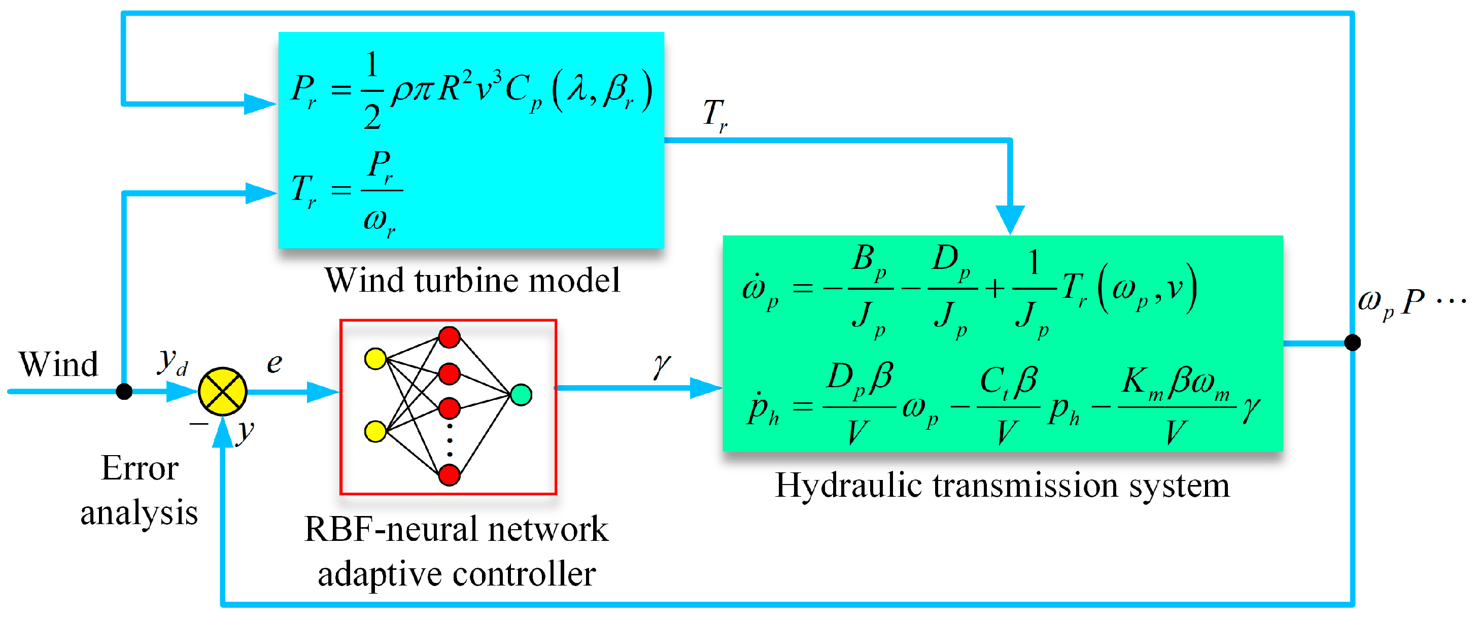
The offshore HWT simulation model shown in Figure 4 was established using MATLAB/Simulink© R2016a software. The simulation model corresponding to paramater l is shown in

Table 3. Parameters of simulation model.

Parameter	Value	Unit
$\rho$	1.225	$\mathrm{kg} {\mathrm{m}}^{-3}$
$R$	3.74	m
$\theta$	0	$\mathrm{rad}$
$B_p$	0.4	${\mathrm{Nmsrad}}^{-1}$
$J_p$	400	$\mathrm{kg} {\mathrm{m}}^{-2}$
$D_p$	$1\times {10}^{-5}$	${\mathrm{m}}^3 {\mathrm{rad}}^{-1}$
$\beta$	$7.43\times {10}^8$	$\mathrm{Pa}$
$C_t$	$6.28\times {10}^{-12}$	${\mathrm{m}}^3 {\mathrm{s}}^{-1} {\mathrm{Pa}}^{-1}$
$V$	$2.8\times {10}^{-3}$	${\mathrm{m}}^3$
$K_m$	$6.366\times {10}^{-6}$	${\mathrm{m}}^3 {\mathrm{rad}}^{-1}$
$C_{p\max }$	0.4496	-
${\lambda }_{\max }$	22.791	-

.

5.1. Simulation Results with Hydraulic Pump Speed as Output

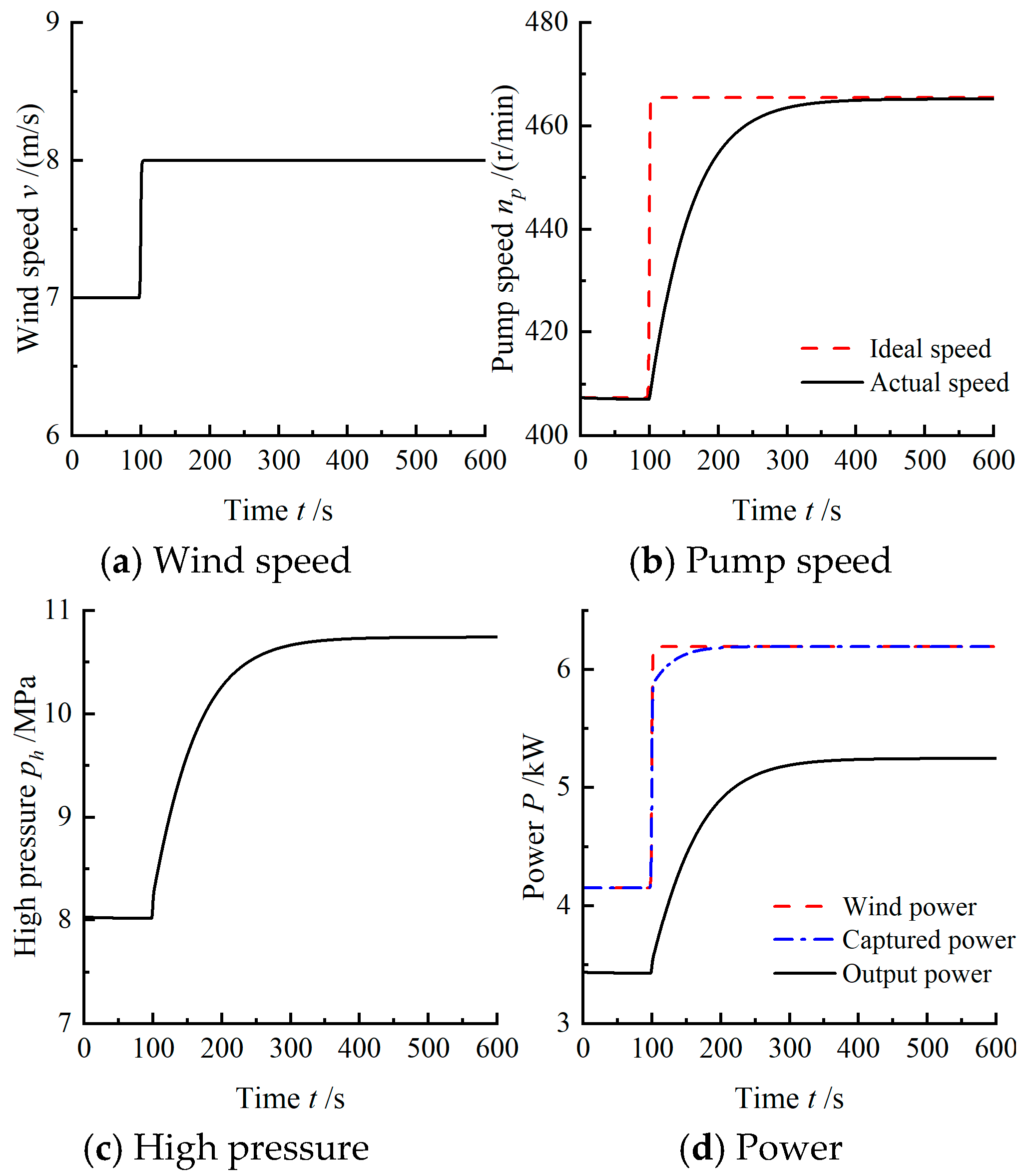
Using the simulation platform, the theory proposed in Section 3 was verified. Under a 7–8 m/s step wind speed, the system responses are observed in Figure 5.

After repeated debugging, the coefficients $K={\left[\begin{array}{cc}100& 20\end{array}\right]}^{\mathrm{T}}$, ${\varsigma }_1=1\times {10}^{-6}$, ${\varsigma }_2=100$. The structure of the RBF neural network is in the form of 2-6-1. The initial value of the weight of the RBF neural network is set to 0. The lower limit of $a$ is 5 and other parameters are set as follows:

$$\begin{gathered} \mathrm{matrix}: c=\left[\begin{array}{c}\begin{array}{ccc}40& 42& \begin{array}{ccc}\begin{array}{cc}44& 46\end{array}& 48& 50\end{array}\end{array}\\ \begin{array}{ccc}-0.5& \begin{array}{ccc}\begin{array}{cc}0.1& 0.7\end{array}& 1.3& 1.9\end{array}& 2.5\end{array}\end{array}\right] \\ \mathrm{width}: b=2. \\ \mathrm{matrix}: Q=\left[\begin{array}{cc}500& 0\\ 0& 500\end{array}\right]. \end{gathered}$$

Additionally, the value of matrix $P$ can be obtained using the command $P=lyap\left(A^{\mathrm{T}},Q\right)$ in MATLAB.

As shown in Figure 5b, when the wind speed varies between 7 m/s and 8 m/s, the actual pump speed can track the ideal speed well under the current wind speed. The wind power captured by the wind turbine rotor can track the maximum wind power well, which is shown in Figure 5d. However, there is a difference between the captured power and output power. The reason is that there is transmission efficiency in the HTS. The energy lost by the HTS mainly includes volume loss, oil heating loss, and so on. The wind power captured by the rotor cannot be converted into electrical energy completely with these unavoidable energy losses.

Seen as Figure 5c,d, the high pressure $p_h$ and the output power of the system have a zero state for about 4 s. The reason is that when the wind speed changes, the control law makes pressure decrease rapidly to ensure that the hydraulic pump has enough acceleration to track the ideal speed, which result in the large fluctuations in the $p_h$ and output power of the system. Nevertheless, in the process of MPPT, it is necessary to ensure that $p_h$ has good dynamic performance while hydraulic pump tracking. So, there is another control strategy with hydraulic pump power as the output proposed in Section 4.

5.2. Simulation Results with Hydraulic Pump Power as Output

Using the same simulation platform, the theory proposed in Section 4 was verified.

After repeated debugging, the coefficients $k_p=1\times {10}^8$, ${\varsigma }_3=1$, ${\varsigma }_4=1$, ${\varsigma }_5=1$. The structure of the RBF neural network is in the form of 2-6-1. The initial value of the weight of RBF neural network is set to 0. The matrix $c$ is defined as $c=\left[\begin{array}{c}\begin{array}{ccc}1& 2& \begin{array}{ccc}\begin{array}{cc}3& 4\end{array}& 5& 6\end{array}\end{array}\\ \begin{array}{ccc}1& \begin{array}{ccc}\begin{array}{cc}2& 3\end{array}& 4& 5\end{array}& 6\end{array}\end{array}\right]$. Additionally, the width $b$ is defined as $b=2$. Also, $\underset{\_}{d}=1000$, which is the lower limit of $d$.

Under a 7–8 m/s step wind speed, the simulation results are shown in Figure 6.

As shown in Figure 6b–d, the ideal speed tracking time and output power are relatively long. Additionally, as shown in Figure 6c,d, the high pressure $p_h$ and the output power do not fluctuate with the hydraulic pump power as output. Although the tracking time is longer, the tracking process is relatively stable and easy to be accepted by the power grid, so it was selected to take the pump power as the HWT MPPT control target. The simulation after this paper is based on the control strategy with hydraulic pump power.

Comparative Simulation under Natural Wind Fluctuation

The wind conditions at sea have complex changes. The MPPT control strategy of HWT must ensure robustness under complex wind conditions.

To analyze the influence of external wind disturbance on the HWT system, a comparison simulation of feedback linearization pump power control with or without RBF neural network adaptive control was made.

The HWT FL-RBFA control law is shown in Equation (47). The control law without the RBF neural network adaptive method can be expressed as [19]

$$\left\{\begin{array}{l}\gamma =\frac{D_p{\omega }_p - C_t{p}_h}{K_m{\omega }_{md}}-\frac{V}{K_m{\omega }_{md}\beta D_p{\omega }_p}\left(v^{*}-D_p{p}_h{\dot{\omega }}_p\right)\\ v^{*}={\dot{y}}_d+k_{1}e+k_2{\displaystyle \int edt}\end{array}\right.$$

(57)

where $k_1=6$, $k_2=4$ [19].

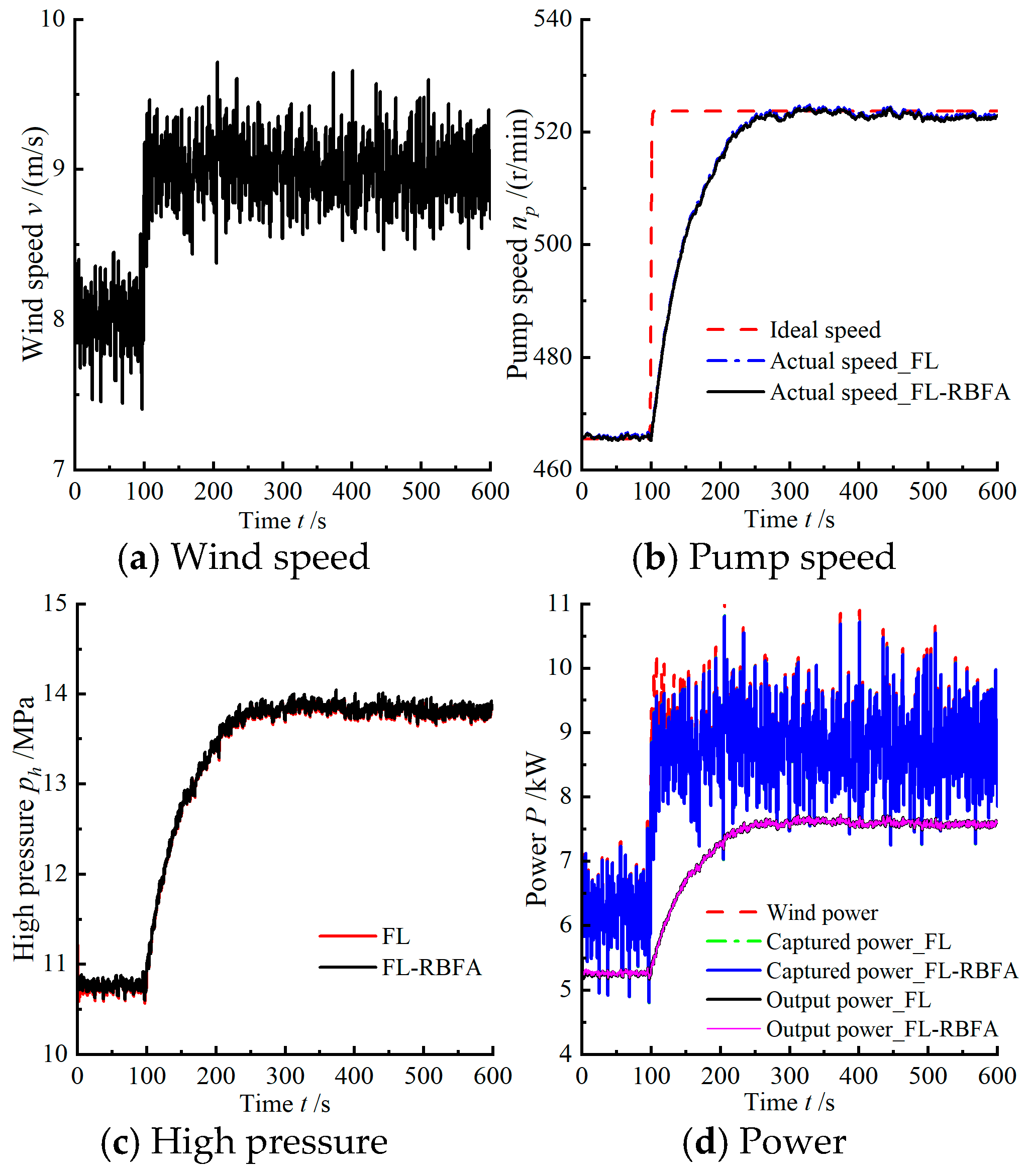
Under the natural wind speed conditions of 8 m/s (±0.5 m/s)~9 m/s (±0.5 m/s) in the simulation, the results are shown in Figure 7.

The simulation results show that the FL-RBFA control law and the theory proposed in Reference [19] have similar control effects in dealing with fluctuating natural wind. Although the wind speed fluctuates, the hydraulic pump can well track the ideal speed under current average wind speed. Moreover, although the wind power captured by the rotor fluctuates greatly, the output power and the high pressure $p_h$ remain steady, which reduces the power grid fluctuation. On the whole, the FL-RBFA control law and the one proposed in Reference [19] both have good external disturbance robustness.

5.3. Comparative Simulation Results under Parameter Uncertainty and External Wind Disturbance Conditions

The parameter uncertainty of the hydraulic transmission system is caused by the inherent characteristics of HTS. The soft parameters such as leakage coefficient $C_t$ and bulk modulus $\beta$ change with the state of the hydraulic transmission system (such as pressure, temperature, etc.). This parameter uncertainty is greatly affected by the large load of the offshore HWT, because this characteristic of offshore HWT causes great pressure in the HTS. So, it is difficult to establish an accurate model required by FL in real application.

The FL control law (57) contains parameters such as $C_t$ and $\beta$. Zhang et al. [35] proposed that the uncertainty of the leak coefficient leads to system vibration and affects the convergence of the system. However, Equation (57) is granted in advance with empirical values, which are not reliable and will vary with working conditions. So, this chapter is to explore the results of different values of $C_t$ in the controller and in the HTS.

The leak coefficient in Equation (57) is defined as $C_t=3.14\times {10}^{-11} {\mathrm{m}}^3 {\mathrm{s}}^{-1} {\mathrm{Pa}}^{-1}$, while the leak coefficient in the HTS is defined as $C_t=6.28\times {10}^{-12} {\mathrm{m}}^3 {\mathrm{s}}^{-1} {\mathrm{Pa}}^{-1}$, which is the reference value shown in Table 2. The simulation results are shown in Figure 8.

As shown in Figure 8, when the leak coefficient in the Equation (57) is different with that in the hydraulic transmission system, the speed of the hydraulic pump (i.e., the speed of the wind turbine rotor), the high pressure $p_h$, and the output power of the system will fluctuate greatly. The whole system is out of control. This means that the MPPT control strategy based solely on FL may lead to system unstability if the empirical values used in the controller are not reliable.

Although both high pressure $p_h$ in Figure 8c and output power in Figure 8d have negative values in the simulation results, this phenomenon does not occur in practice, because there are hydraulic oil compensators in real hydraulic systems.

The improved FL-RBFA control strategy proposed in this research approximates the nonlinear model through a RBF neural network without relying on accurate mathematical expression. The system instability caused by inherent parameter uncertainty is avoided, seen in Figure 8.

If other parameters in Equation (57) are individually changed, such as increasing $\beta$ or $V$ to 10 times the reference value in Table 2 or decreasing it to one tenth, the system performance using only the feedback linearization method is similar to that in Figure 6 and will not obtain out-of-control results. At present, there is no effective method to determine the specific value of $C_t$, $\beta$, and $V$ in practical engineering application. Therefore, the RBF neural network adaptive control strategy proposed in this research has certain engineering significance.

Finally, we might as well check the performance of the FL-RBFA control strategy (47) under extreme conditions. Assuming that the natural wind speed change (7 ± 0.5~8 ± 0.5 m/s) and the leakage coefficient in the HTS meet the sinusoidal law, that is, $C_t=5\times 6.28\times {10}^{-12}\sin \left(\pi t\right)$ ($C_t$ will not change according to this law in practice), the simulation results are shown in Figure 9.

It can be concluded from Figure 9 that the FL-RBFA control strategy can ensure the stability and robustness of the system under the severe combined condition of external and internal disturbances.

Moreover, it should be noted that the acceleration signal ${\dot{\omega }}_p$ used in (57) may introduce high-frequency measurement noise into the system and an add-on cost of wind turbines [36]. Nevertheless, the control strategy (47) is immune to this problem for not using differential signals.

6. Conclusions

This paper focuses on solving the maximum power point tracking control problem of offshore hydraulic wind turbine affine nonlinear systems with parameter uncertainty. Taking the hydraulic pump speed and hydraulic pump power as outputs, the feedback linearization method combined with the RBF neural network adaptive maximum power point tracking control strategy was applied, respectively.

By means of simulation, the maximum power point tracking control performance with pump speed and pump power as output were compared. The power control performance is better than the speed control. Specifically, there is no large fluctuation in the high pressure and output power, which is more friendly to the power grid.

In natural wind conditions, the hydraulic pump power control strategy shows good robustness towards external disturbance. While dealing with the internal disturbance, the feedback linearization–RBF neural network adaptive maximum power point tracking control strategy’s performance is far better than that of feedback linearization only. Feedback linearization only will make the system out of control. By contrast, the feedback linearization–RBF neural network adaptive maximum power point tracking strategy with pump power as the control target is effective and robust against different kinds of disturbance, which has significant value in the hydraulic wind turbine engineering application.

Because a RBF neural network is used to approximate the unknown term, this paper does not consider how the uncertain parameters of hydraulic transmission fluctuate. If the uncertain parameters can be transmitted to the controller through the real-time parameter identification strategy, this should also serve as an interesting research direction.