A Generic Model for Accurate Energy Estimation of Electric Vehicles

Abstract

A systematic simulation model is proposed in this research paper to estimate the energy consumption of electric vehicles. The main advantage of this model is that it is made in a generic and simplified way in order to be adaptable to different electric vehicles. The overall electrical power corresponding to the performed maneuver is estimated considering: a tabular form of electric motor efficiency, mechanical power losses, a generalized efficiency map of the power electronics, the auxiliary power losses, and an electro-thermal Lithium-Ion battery pack model. The battery model was developed in a previous work, which simulates the open circuit voltage curves at different temperatures and the alteration in the internal resistance of the battery cells. The proposed model is validated with experimental data from the maneuver tests. The battery model proved high accuracy in estimating the voltage values relevant to the WLTP2 driving cycle on the chassis roller test bench. Furthermore, the mechanical and electrical power were estimated with excellent matching compared to actual test field driving test measurements, giving only the measured vehicle speed and auxiliary power losses. Finally, the state of charge change is predicted accurately along the performed test field dynamic maneuver.

1. Introduction

The topics of energy consumption (customer-driven) and emission reduction (politically driven) are two essential goals for automotive development [1]. In addition, practical solutions for major challenges of trip-level management need to be provided. Thus, the electrification of commercial, public, and freight delivery vehicles has become essential [2,3]. Electric vehicles (EVs) have been widely adopted in recent years due to the growing attention regarding implementing environmentally friendly energy sources and energy conservation issues [4]. The most popular technologies that have adopted electrical powertrains are hybrid electric vehicles (HEVs), plug-in hybrid electric vehicles (PHEVs), battery electric vehicles (BEVs), and fuel cell electric vehicles (FCEVs) [5].

A comparative study between the energy consumption of conventional internal combustion engines and electric vehicles was performed in [6]. The comparison was made between two diesel-engine vehicles and their electric-equivalent models. An actual route in a mountain region was simulated to estimate the energy consumption of each vehicle model. The results from the simulation models were evaluated for different scenarios and driving cycles. Although the electric vehicles were heavier than their equivalent internal combustion engine (ICE) cars, they consumed less energy due to the regenerative braking function of electric cars. Regarding energy efficiency, a BEV performs much better than an ICE vehicle. Provided the high BEV efficiency in energy production, their overall efficiency can reach up to twice that of ICE cars [7]. Moreover, electric motors can provide a high torque for wide-ranging rotational speed. Hence, a single-gear transmission is necessitated, which improves the powertrain’s efficiency even more. Generally, a BEV contains fewer rotating parts than an ICE vehicle, resulting in lower maintenance costs [8]. Estimating the remaining driving range of EVs and precise estimation of the battery’s state of charge (SOC) are popular areas of study [7,9,10,11,12,13,14,15,16]. A comprehensive survey was made in [10] to investigate the influencing factors for the remaining driving range of EVs. The authors classified the influential factors into five categories: route and terrain, weather and environment, driving behavior, vehicle modeling, and battery modeling. An experimental investigation of the energy consumption in electric vehicles is presented in [11], based on driving course type, driving style, and ambient temperature. The remaining driving range is a sophisticated concept affected by multiple factors complicating its estimation. The vehicle’s driving conditions primarily include the speed profiles and the altitude curves. Vehicle speeds and altitude changes are determined based on information such as driving routes, driver’s behavior, road traffic, environment conditions, and vehicle dynamics models [17].

Several research projects are oriented to establish accurate energy consumption estimations that achieve the optimal energy economy to drive to a particular destination by modeling the driving condition, considering driving style and selecting the optimal driving route [18]. Likewise, the authors of [19] developed a mathematical regression model for vehicle energy consumption based on eight different test vehicles’ instantaneous speed and acceleration measurements. The authors considered various influential factors on energy consumption: the roadway grade and roughness, the vehicle’s interaction with the traffic, and the driver’s behavior. Developing energy estimation algorithms under realistic conditions has become imperative. Subsequently, various concepts have been adopted to calculate the accumulated energy consumption during real driving routes. Some methods are based on sparse GPS observations [20], where readings from 68 EVs were used in a linear regression approach to calibrate an energy consumption prediction model. Some other approaches adapted to kinetic and potential energy changes during the trip, as in [21], in which a measured and estimated energy consumption process in a customized conversion electric vehicle was realized by collecting the data for energy consumption for different routes with alternating driving modes. Another approach for energy consumption modeling, which is oriented to quantify correlations between energy consumption in electric vehicles and its kinematic parameters using real-world data, was developed in [22]. Prediction of the driving conditions can be classified into two methods, according to the availability of the driving destination information [17]: First, if the destination is known, the vehicle speed profile and the altitude changes are evaluated based on the future route segment information. Route segment information is divided into fixed parameters, including road speed limit and altitude data, while real-time data provide information on road adhesion, traffic jams, and weather conditions. Second, if the destination is unknown, stochastic models are used to predict the virtual driving conditions by employing the stored statistical data of the vehicle in the present area to estimate vehicle energy consumption. An interesting method for a stochastic model that connects the vehicle with the data cloud to predict the remaining driving range is presented in [23]. The authors’ concept was based on estimating the remaining discharge energy in the battery by predicting the forthcoming operating conditions. The results showed that the proposed vehicle–cloud collaboration solution could improve the accuracy of the remaining driving range within an accuracy of 5%.

Two main approaches are used to model EVs [24]. The first is forward modeling, also known as the “dynamic approach”. The second is backward modeling, also known as the “quasi-static approach”. The forward approach concerns equations for the behavior of powertrain components and their dynamic interaction. On the other hand, the backward approach considers determining the forces acting on the wheels based on an input reference speed profile. Then, to process backward over the powertrain components. After that, the motor torque is computed, and the battery’s energy needed to drive the electric motor is determined. The choice between the forward and backward methods depends on the study’s objective. For instance, the forward method does not require a reference driving speed profile but a control part. Moreover, it is based on solving the model’s differential equations, making it more precise at the expense of more significant computational effort than the backward approach. The backward method is based on analytical models considering vehicle dynamics and powertrain loss estimation from available efficiency maps [25]. In general, computational models require more processing than analytical models. However, they are more precise as they operate based on data analysis and prediction. In addition, analytical models can only respond to changes in vehicle performance as they are vehicle dynamics-dependent and based on physical modeling. More details about the advantages and disadvantages of these approaches are available in [26,27].

The authors of [7] presented a sensitivity analysis for the energy demand estimation of battery electric vehicles. Their model is based on modeling mechanical quantities, such as driving resistances and losses in the powertrain. They found that the factors with the highest impact on the energy demand estimation accuracy are the uncertainty of powertrain efficiency and rolling friction coefficient. Moreover, the test results showed that the uncertainty of auxiliary power demand, especially for heating and cooling, substantially affects the estimation accuracy at low speeds. The authors in [27] stressed the importance of an accurate power-based EV energy consumption model. Their EV model was created using MATLAB/Simulink software (https://www.mathworks.com/products/simulink.html, accessed on 10 January 2024) based on an actual EV, the BMW i3. The EV forward simulation model comprised a powertrain system, longitudinal vehicle dynamics, and a driver model. The efficiency maps of the electric motor and the power electronics were created from the available technical data of the test vehicle. The input to their EV model was a reference speed that the driver model tracked. They validated their model using standard driving cycles, entirely in simulation and without field tests. Nonetheless, the motor and power electronics efficiency maps are specifically for the selected EV. Moreover, the used battery model is a simplified one with constant parameters.

The battery system is one of the most vital components of an electric vehicle. Among energy storage technology development, lithium-ion batteries (LiBs) are the most promising solution compared to the other available energy storage technologies [14] due to their distinctive benefits, such as their high energy density, low maintenance, and long life span [27]. SOC indicates the battery’s remaining charge. It is crucial to have an accurate battery SOC estimation model as LiBs are sensitive to both over-charging and over-discharging, creating the demand to predict the SOC with the highest accuracy possible [12]. The authors of [7] classified the SOC estimation methods into five categories of battery modeling: tank model, empirical model, lumped-parameter equivalent circuit models (ECMs), machine learning model, and electrochemical model-based estimation. ECM-based estimation is the most widely used model for online vehicle applications. ECM should enable simulating an actual LiB voltage according to any current excitation. However, in reality, some characteristics of the LiBs might not be adequately represented by circuit elements, such as the hysteresis effect.

The authors developed a second-by-second model with regression coefficients depending on instantaneous speed, acceleration, and SOC. The developed model encloses four driving modes: acceleration, deceleration, cruising, and idling. Likewise, in [13], the developed models have regression parameters that were attained based on the aggregated data from real-world trips, which was extended in [28] by creating a multiple linear regression model to estimate energy consumption. Many other studies reviewed the latest SOC estimation methods to define the pros and cons of each approach, including physical modeling state estimation [14,15] or Artificial Intelligence techniques [12,15]. Moreover, the authors added a neural network model to predict driving parameters. In a similar context, a model to estimate the energy consumption of EVs is proposed in [29]. The authors of [11] benefit from the acceleration distribution and altitude difference. They are classified as positive kinetic energy, relative positive acceleration, and the standard deviation of the variation of the battery. In [30], an adaptive multi-resolution approach was proposed for real-time energy consumption estimation in electric vehicles. A two-step nonlinear iterative algorithm approximates three key parameters: powertrain efficiency, wind speed, and rolling resistance. The first step is linear estimating with a Kalman filter, whereas the second step follows a nonlinear optimization search.

Empirical open circuit voltage (OCV) modeling and look-up table interpolation are responsible for low computational complexity. The direct OCV-based SOC estimation method has minor computational complexity and a relatively high accuracy. Hence, it is ordinarily used as a calibration methodology. By using the OCV estimation method, especially combined with the ECM model, OCV-based SOC estimation enables extension to dynamic working conditions [7]. It is also essential that the OCV curve is entirely consistent for all LiBs, which allows the use of the experimental curves for online estimation applications. Therefore, OCV-based estimation is an extensively practical method for online applications. Even though the OCV characteristic curves are relatively stable for Lithium-ion batteries, they alternate with the cycle life and temperature [30,31]. Therefore, to have a reliable SOC-OCV relationship, it is essential to have experimental data for the influence of temperature and cycle life [15]. The error in SOC when implementing OCV-based estimation methods is smaller than that of the other methods, as shown in Figure 1. Although the OCV area is located in the online feasible region, special attention should be given to the influences of temperature, aging, and hysteresis [16]. Our previous work [32] solved these issues; an OCV empirical model is integrated with an ECM as a function of the SOC and battery’s temperature. The elements of the internal resistance model are also functions of the SOC and battery’s temperature. The hysteresis during discharging and charging is modeled, as well. In addition, the capacity fading effect, which represents the aging factor, is embedded in the ECM model. Highly dynamic maneuvers of real-world tests are modeled with high accuracy. Based on these results and the investigation in [33], the proposed model in [33] makes an excellent choice for the LiB model for this work.

The presented research emphasizes significant factors in EV energy consumption estimation accuracy, such as developing detailed vehicle dynamic models, estimating high-resolution powertrain efficiency, and considering environmental effects along a specific route. So far, these works consider procedures too complicated to obtain representative models for the energy consumption of EVs or more straightforward methods that are developed but with less accurate results. On the other hand, this research proposes a generic modeling approach that overcomes the downsides of the resented works.

Section 2 defines the efficiency map model for different electric motor sizes, and an approximated efficiency map for the power electronics is displayed. Section 3 summarizes the proposed battery model in one of our previous works [32]. This detailed battery model is an excellent asset for enhancing the accuracy of the estimation results. Then, Section 4 describes creating the complete vehicle model, including the battery model. The main advantage of this model is that it defines a systematic and straightforward procedure to model the energy consumption and the change in the battery-pack state of charge for electric vehicles. The model inputs are a specific maneuver’s measured speed, the measured SOC, and auxiliary power consumption to predict the corresponding energy consumption. Then, the model is validated with actual measurements on the test vehicle. Auxiliary devices are additionally included in the model as they can extensively influence the accuracy of energy consumption estimation [15]. Moreover, our work is adapted for a wide range of motors and power electronics.

2. Estimating Power Losses in Electric Powertrain

A computational model for energy consumption in EVs is proposed in [34]. The authors used a simplified battery model based on technical data. The model’s accuracy was endorsed by incorporating explicit equations for electric machines to generate efficiency curves for each motor and generator modes. In this work, the model introduced in [34] will be enhanced by incorporating more detailed powertrain and battery models.

As a general rule, electric motors are designed to operate between 50 and 100% of their rated load. The highest operating efficiency reaches roughly 75% of the full load, while the motor efficiency decreases significantly at loads below 50%. The part-load efficiency curves are displayed in Figure 2 for electric motors with different sizes [35]. The motor efficiency can be estimated in correspondence to the fraction (x) of the motor’s mechanical output power (P_mo) regarding the rated motor power (P_mr) in kW, i.e., x = 0.001|P_mo|/P_mr [34]. Equation (1) describes the electrical machine efficiency for both motor mode (η_mot) and generator mode (η_gen).

$$efficiency\left(x\right)=\left\{\begin{array}{cc}\frac{cout1 x + cout2}{x + cout3} ,\hfill & 0\le x<0.25\\ dout1 x+dout2 ,& 0.25\le x<0.75\\ eout1 x+eout2 ,& x\ge 0.75\end{array}\right.$$

(1)

The coefficients in Equation (1) are selected for an asynchronous motor with a rated power of 45 kW, i.e., the yellow curve in Figure 2, which is the test vehicle in this work. These coefficients are acquired from [34], which implemented curve fitting of many motors, and are presented in

Table 1. Coefficients for determining efficiency in Equation (1) [34].

	Induction Electric Machine		Synchronous Electric Machine
Coefficient	Motor Mode	Generator Mode	Motor Mode	Generator Mode
cout1	0.924300	0.925473	0.942269	0.942545
cout2	0.000127	0.000148	0.000061	0.000067
cout3	0.012730	0.014849	0.006118	0.006732
dout1	0.080000	0.075312	0.060000	0.057945
dout2	0.860000	0.858605	0.905000	0.904254
eout1	−0.073600	−0.062602	−0.076000	−0.066751
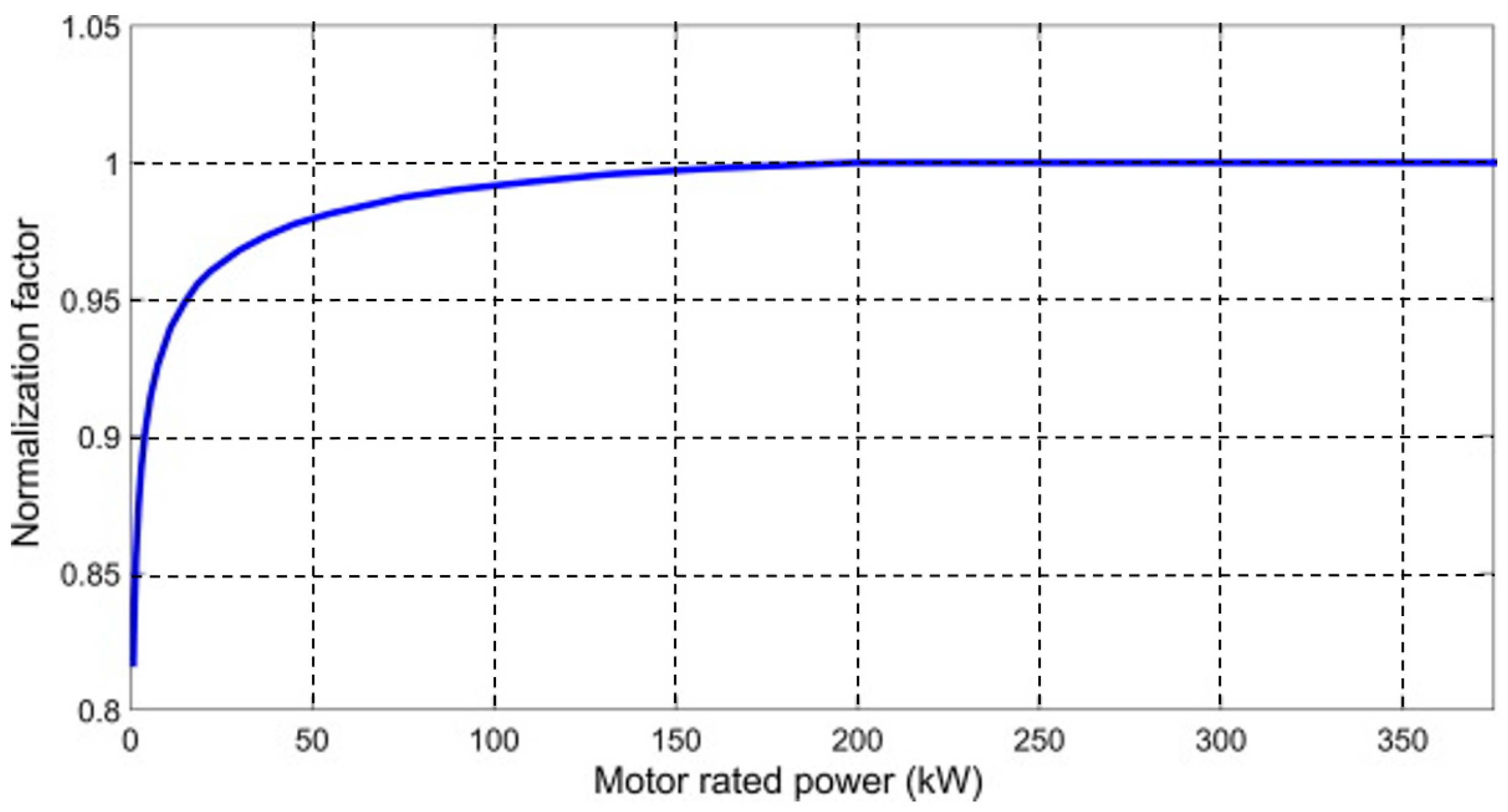
eout2	0.975200	0.971034	1.007000	1.002698

. One of the main characteristics of electrical machines is that their efficiency increases with size [36]. Therefore, when determining the electrical machine efficiency given the output power, the efficiency must first be calculated from Equation (1), and then the efficiency is multiplied by a normalization factor (f_norm). In case of regenerative braking, the efficiency is multiplied by a regenerative normalization factor (f_regen), as described in [34]. Figure 3 shows the efficiency normalization factor values based on rated output power. According to this relation, the f_norm for a 45 kW motor equals 0.978.

The mechanical losses in the total gear transmission efficiency (η_g) are also a significant factor [37]. Therefore, the authors of [25] created an energy consumption model for EVs considering a deceleration-dependent regenerative braking efficiency model. They also validated their model with measurements from different electric vehicles performing several typical driving cycles. In addition to the energy consumption from traction, the consumption of the auxiliary devices in electric vehicles is significant [18]. The authors of [13] analyzed the influence of auxiliary devices’ load on energy consumption at three different ambient temperatures. Accordingly, the total battery output power should also cover the auxiliary load power (P_aux) and the motor’s power or obtain the generator’s electrical power. The power consumption of the auxiliary systems can significantly influence the overall energy consumption of EVs. For this reason, they must be included in the vehicle model for more accurate energy consumption estimation [27,38]. Several factors can determine the energy consumption due to the auxiliary devices. Consequently, some auxiliary devices are deactivated during the test runs to reduce the uncertainty in auxiliary power estimation [4]. For simplicity, average values are selected to represent the average power of each auxiliary device in an EV and their consumption. Then, their effective power consumption during the tests is estimated based on each device’s activated intervals [27]. In [34], the power model is modified with a correction factor constant to consider the battery efficiency drop during the round trip. In this work, a detailed physical battery model is employed instead, which incorporates more variable loss factors and provides the final battery voltage.

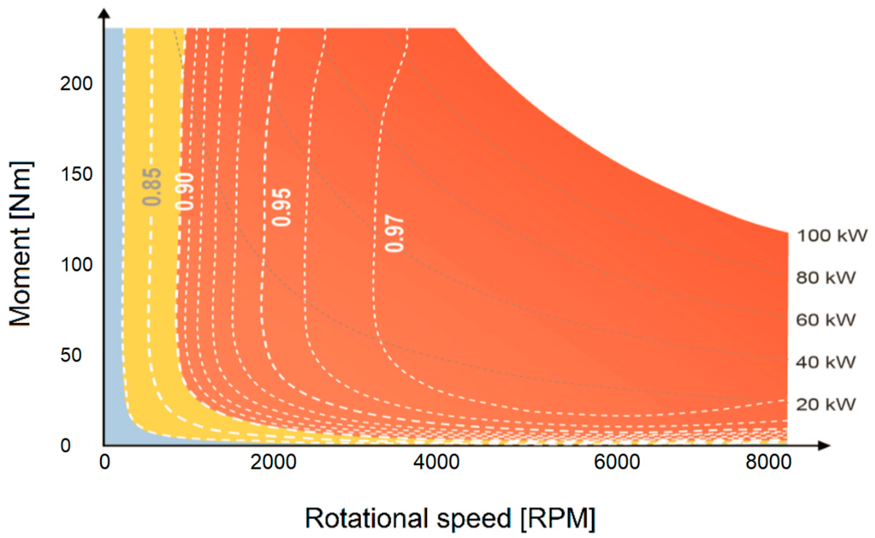
The conversion of the battery’s direct current into a three-phase current for the motor is associated with losses within the power electronics. Therefore, the efficiency of the power electronics (η_pe) can be mapped analogously to the electric machine efficiency map, as shown in Figure 4. The data in this figure represent different sizes of motors within a range of power from 20 to 100 kW [39]. The asynchronous machine specifications of the front-wheel-drive vehicle under the test (VUT) are listed in

Table 2. Technical data of LiFePO₄ battery [40].

Parameter [Unit]	Value
Nominal Module Voltage [V]	19.2
Nominal Module Capacity [Ah]	69
Max Continuous Load Current [A]	120
Peak Current for 30 s [A]	200

.

3. Battery Model

The battery pack of the VUT contains 19 battery modules. Each module encompasses six cell blocks that are connected in series. Every cell is made of 50 LiFePO₄–graphite cells connected in parallel. The total number of cells within the single battery module is 300 [32]. The battery module specifications are given in Table 2. The VUT provides battery cell units of cathode lithium iron phosphate (LiFePO₄). These cells are distinguished by their open-circuit voltage curves that remain almost constant over the SOC range from 20% to 80%, even at different ambient temperatures [32]. The same model developed in [32], which accurately simulates the changes in the battery during dynamic maneuvers, will also be employed in this work. The battery model requires the following inputs: the battery current, the SOC signal, the corresponding capacity rates (C-rate), the ambient and battery temperatures, and the number of charging and discharging cycles.

The proposed open-circuit voltage (V_OC) model in [32], as a function of the battery SOC and temperature, is represented by Equations (2) and (3). According to [41], the open voltage is modeled by separate equations in case of discharging, i.e., V_OC,dis, and charging, i.e., V_OC,ch. The corresponding constant values are given in

Table 3. VOC parameter values [32].

Constant	Value	Constant	Value
a1	−1.166	b1	−0.9135
a2	−35	b2	−35
a3	3.344	b3	3.484
a4	0.1102	b4	0.1102
a5	−0.1718	b5	−0.1718
a6	−2 × 10−3	b6	−8 × 10−3
dVOC,d/dT	0.00125	dVOC,c/dT	0.00069

. The effect of the temperature on the discharge and charge curves over SOC are considered through the constant gradients dV_OC,d/dT and dV_OC,c/dT, respectively.

$$V_{OC,dis}\left(SOC,T\right)=a_1{ e}^{-a_2 SOC}+a_3+a_4 SOC+a_5{ e}^{-\frac{a_6}{1-SOC}}+T_{batt}\frac{d{V}_{OC,d}}{dT}$$

(2)

$$V_{OC,ch}\left(SOC,T\right)=b_1{ e}^{-b_2 SOC}+b_3+b_4 SOC+b_5{ e}^{-\frac{b_6}{1-SOC}}+T_{batt}\frac{d{V}_{OC,c}}{dT}$$

(3)

By neglecting the temperature differences between the cells in the same battery module, the temperature variations in the battery module (T_batt) can be described in Equation (4) [42].

$$M_{batt}{C}_p\frac{d{T}_{batt}}{dt}=I_{batt}\left(V_{OC}-V_{batt}\right)-h{A}_{batt}∆T-\epsilon \mathsf{\sigma }{A}_{batt}\left(T_{cell}^4-T_{amp}^4\right)$$

(4)

where ΔT is the temperature difference between the battery cell and the ambient (T_cell − T_amp), I_batt is the battery input current, and V_batt is the battery output voltage. The constants of Equation (4) are defined and evaluated in

Table 4. Battery thermal model parameter list [32].

Parameter	Description	Value	Unit
Abatt	Battery module surface area	0.284	m2
Mbatt	Battery module mass	12	kg
Cp	Specific heat capacity	1360	J·kg−1·K−1
σ	Stefan–Boltzmann constant	5.67 × 10−8	W·m−2·K4
ε	Emissivity of heat	0.95	-
h	Natural heat convection constant	4	W·m−2·K−1

. The battery circuit model considers the fading capacity effect by adding resistance in series (R_cyc). It is identified in [42], as shown in Equation (5), as a function of the number of charging and discharging cycles (n_cyc). The usable battery capacity (C_usable) is a function of n_cyc and temperature [43]. Figure 5 shows the percentage of C_usable from the initial capacity (C₀) over the n_cyc and at a reference ambient temperature of 23 °C. A simple definition for the change in SOC is made by Equation (6) [42], where SOC₀ is the initial state of charge.

$$R_{cyc}=0.0015 {\left(n_{cyc}\right)}^{0.5}$$

(5)

$$SOC={SOC}_0-\int \left(I_{batt}/C_{usable}\right)dt$$

(6)

The values of the internal resistance components of resistances and capacitors are determined through Equations (7)–(11), which are developed in [44], where ϑ is the battery cell temperature [°K], and the constant, c₁–c₃₉, values are listed in

Table 5. Constant values of Equations (7)–(11) [44].

Constant	Value	Constant	Value
c1	1.080 × 10−2	c21	−6.919 × 10−1
c2	−11.03	c22	2.902 × 10−1
c3	1.827 × 10−2	c23	2.130 × 106
c4	−6.462 × 10−3	c24	−6.007 × 106
c5	−3.697 × 10−4	c25	6.271 × 106
c6	2.225 × 10−4	c26	−2.958 × 106
c7	1.697 × 102	c27	5.998 × 105
c8	−1.007 × 103	c28	−3.102 × 104
c9	1.408 × 103	c29	2.232 × 103
c10	3.897 × 102	c30	3.128 × 103
c11	−6.580	c31	−2.398 × 103
c12	12.11	c32	1.298 × 10−1
c13	2.950 × 10−1	c33	−2.892 × 10−1
c14	−20.00	c34	2.273 × 10−1
c15	4.722 × 10−2	c35	−7.216 × 10−2
c16	−2.420 × 10−2	c36	8.980 × 10−2
c17	6.718 × 10−3	c37	7.613 × 10−1
c18	−20.00	c38	10.14
c19	−5.967 × 10−4	c39	2.608 × 102
c20	6.993 × 10−1

. The total estimated battery output voltage (V_batt) is modeled as in Equations (12) and (13) [32]. According to [41], the hysteresis effect between the discharge and charge behaviors is considered in V_batt by implementing two different equations, i.e., (12) for discharging and (13) for charging. The parameters in Equations (12) and (13) are defined and evaluated in

Table 6. Parameters list of the battery discharge voltage model [41].

Parameter	Description	Value
K	Polarization constant or polarization resistance	0.012
Q	Battery capacity	Variable
A	Exponential zone amplitude	0.271
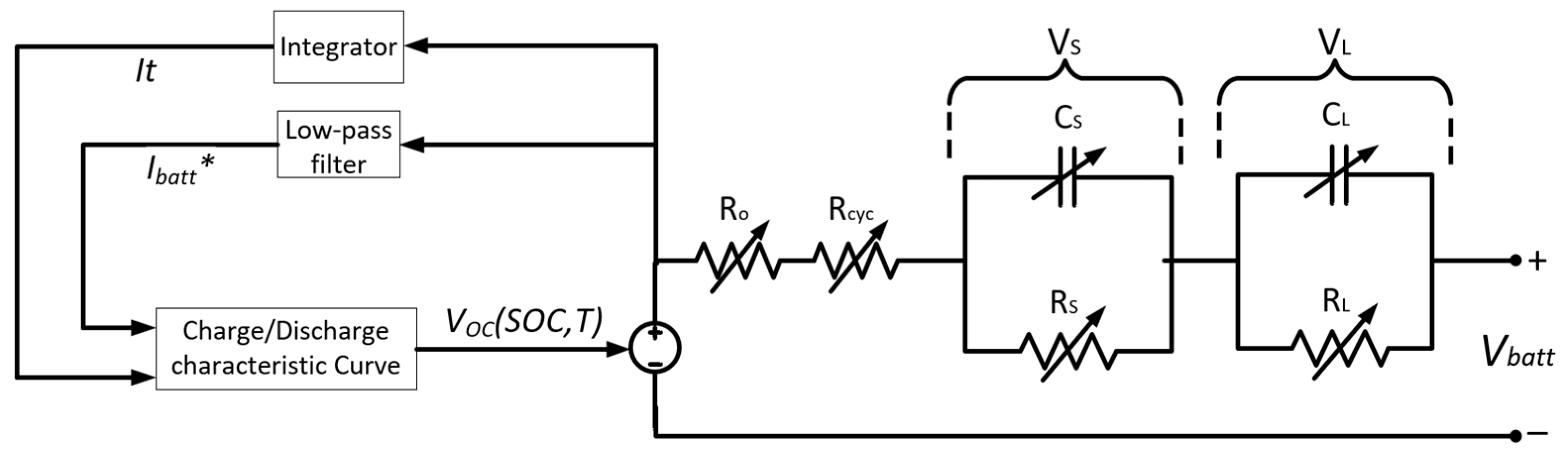
B	Exponential zone time constant inverse	152.130

. The battery internal resistance parameters in Equation (14) are acquired by multiplying the corresponding battery cell internal resistance parameter, calculated by Equations (7)–(11), by the total number of cells. The battery circuit model diagram is shown in Figure 6. I_batt is the battery current, I^*_batt is the filtered battery current, and It is the integration of the battery current. The charge–discharge characteristics are considered, and hysteresis is modeled with empirical equations. The open-circuit voltage, V_OC(SOC,T), is employed as a function of SOC and temperature. The aging effect is regarded by adding R_cyc to the internal resistance. The variable ohmic resistance R_o and two variable RC networks, R_SC_S and R_LC_L, are also considered for the short- and the long-time transient responses, respectively.

$$R_{s, cell}\left(SOC,\vartheta \right)=\left(c_1{e}^{\left(c_{2}SOC\right)}+c_3+c_{4}SOC\right)+c_5∆\vartheta +c_6 SOC ∆\vartheta$$

(7)

$$C_{s, cell}\left(SOC,\vartheta \right)=\left(c_7{SOC}^3+c_8{SOC}^2+c_{9}SOC+c_{10}\right)+c_{11}SOC ∆\vartheta +c_{12}∆\vartheta$$

(8)

$$R_{l, cell}\left(SOC,\vartheta ,I_{C-rate}\right)=\left(\left(c_{13}{e}^{\left(c_{14}SOC\right)}+c_{15}+c_{16}SOC\right)+c_{17}∆\vartheta e^{\left(c_{18}SOC\right)}+c_{19} ∆\vartheta \right)\times \left(c_{20} {\left(I_{C-rate}\right)}^{c_{21}}+c_{22}\right)$$

(9)

$$C_{l, cell}\left(SOC,\vartheta \right)=\left(c_{23}{SOC}^6+c_{24}{SOC}^5+c_{25}{SOC}^4+c_{26}{SOC}^3+c_{27}{SOC}^2+c_{28}SOC+c_{29}\right)+c_{30}{e}^{\frac{c_{31}}{\vartheta }}$$

(10)

$$R_{o, cell}\left(SOC,\vartheta \right)=\left(c_{32}{SOC}^4+c_{33}{SOC}^3+c_{34}{SOC}^2+c_{35}SOC+c_{36}\right)c_{37}{e}^{\frac{c_{38}}{\vartheta -c_{39}}}$$

(11)

$$V_{batt}=V_{OC,dis}\left(SOC,T\right)-\left(R_O+R_{cyc}+V_S+V_L\right)·I_{batt}-K\frac{Q}{Q-It}·\left(It+I_{batt}^{*}\right)+A{e}^{-B·It}$$

(12)

$$V_{batt}=V_{OC,ch}\left(SOC,T\right)-\left(R_O+R_{cyc}+V_S+V_L\right)·I_{batt}-K\frac{Q}{It-0.1Q}·I_{batt}^{*}-K\frac{Q}{Q-It}·It+A{e}^{-B·It}$$

(13)

$$\begin{array}{c}\frac{d{V}_S}{dt}=\frac{I_{batt}}{C_S}-\frac{V_S}{{R_{S}C}_S}\\ \frac{d{V}_L}{dt}=\frac{I_{batt}}{C_L}-\frac{V_L}{{R_{L}C}_L}\end{array}$$

(14)

4. Integration and Validation of the Complete Vehicle Model

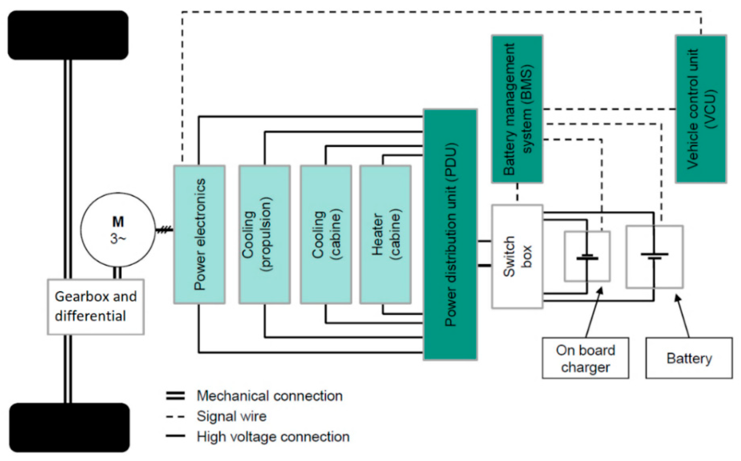
The electric VUT used for this work is shown in Figure 7. Actual maneuver test measurements from this vehicle will be used to validate the proposed simulation models. The vehicle’s motor is powered by alternating current (AC), which is delivered from the power electronics that convert the direct current (DC) of the battery. The battery management system (BMS) controls the processes of battery charging and discharging. Moreover, it monitors the temperatures of each battery pack’s cell blocks. The “torque demand” signal is determined in correspondence with the actuation of the accelerator pedal position. This signal is then manipulated by the vehicle control unit (VCU) based on the car’s current driving state, battery state, motor, and pedals. The front-wheel-driven VUT powertrain topology is shown in Figure 8. Except for the battery and the mechanical parts, none of these systems are modeled in this work because we considered the backward modeling approach. Moreover, no cabinet heating or cooling is activated during the tests in this work.

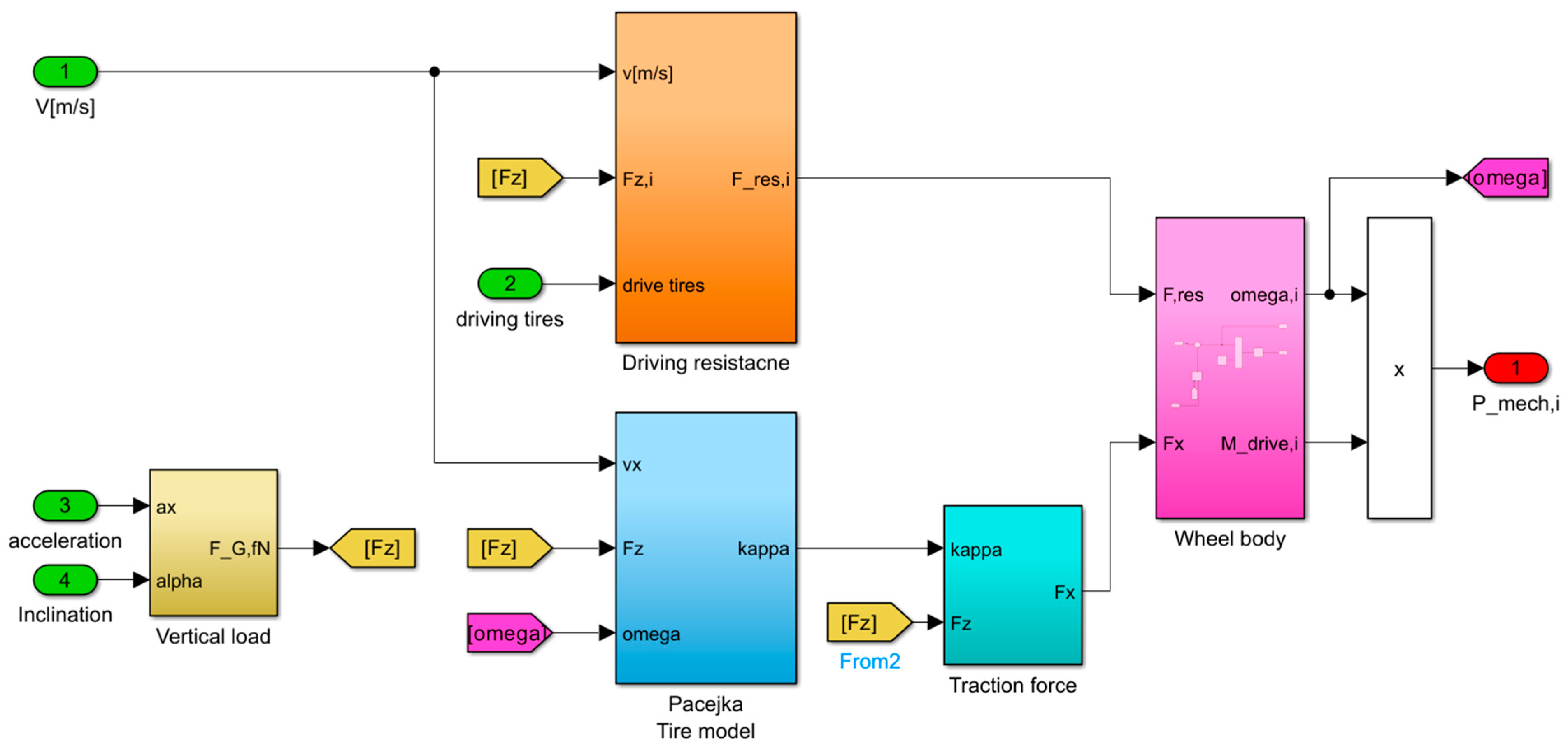
The simulated P_mech is obtained from the vehicle dynamic simulation model, illustrated in Figure 9. The model has three inputs: the vehicle’s speed, acceleration, and inclination. The output is the P_mech, which results from the interaction between the driving resistance force and traction force on the corresponding wheel model. The slip tire model increases the realism of the model. Figure 10 shows the battery simulation model proposed in [33]. The implemented parameters in the VUT model are listed in

Table 7. Parameters list for the VUT dynamic model.

Description	Value	Unit
Vehicle mass	1528	kg
Moment of inertia about the longitudinal axis	482.70	kg.m2
Moment of inertia about the vertical axis	2585.60	kg.m2
Wheelbase	2.59	m
Distance between center of gravity—front axle	1.47	m
Distance between center of gravity—rear axle	1.11	m
Height of the vehicle’s center of gravity	0.45	m
Transmission gear ratio	4	-
Differential gear ratio	2.5	-
Vehicle engine/motor inertia	0.03	kg.m2
Front axle inertia	3.7 × 10−3	kg.m2
Rear axle inertia	3.7 × 10−3	kg.m2
Tire inertia	0.1	kg.m2
Wheel hub inertia	0.124	kg.m2
The height of the vehicle’s rolling center	0.31	m
Half-track width between front wheels or rear wheels	0.78	m
Distances of the front suspension from the middle	0.78	m
Distances of the front damper from the middle	0.78	m
Distances of the rear suspension from the middle	0.78	m
Distances of the rear damper	0.78	m
Spring stiffness front	21,269	N/m
Damping coefficient front	2244.4	N.s/m
Stiffness of the front anti-roll bar	7018.8	N.m/rad
Spring stiffness rear	17,374	N/m
Damping coefficient rear	1550.6	N.s/m
Longitudinal force initial slope in Pacejka formula	23.64	-
Longitudinal force shape factor in Pacejka formula	1.35	-
Longitudinal force peak factor in Pacejka magic formula	0.90	-
Longitudinal force curvature factor in Pacejka formula	1.37	-
Aligning initial torque slope in Pacejka formula	16.37	-
Aligning torque shape factor in Pacejka formula	1.13	-
Aligning torque peak factor in Pacejka magic formula	0.13	-
Aligning torque curvature factor in Pacejka formula	0.89	-
Tire effective rolling radius	0.31	m
Tire longitudinal stiffness factor (related to the wheel load)	19.15	1/m
Tire longitudinal nominal relaxation length	1.5	m
Tire minimum relaxation length	0.05	m

.

The complete model of the VUT is shown in Figure 11. The main gain of this model is its ability to estimate the total battery power for the assigned maneuver based on two input variables: the relevant speed profile (V_x) and auxiliary power (P_aux). Based on the speed profile, the corresponding physical quantities are determined from a simulation model for the VUT. Then, the mechanical power (P_mech) can be estimated using Equation (15) [45].

$$P_{mech}={\sum }_1^4{M}_{drive,i} {\omega }_i$$

(15)

where M_drive,i is the driving moment on the wheel hub, and ω_i is the corresponding wheel’s angular speed. The P_mech sign decides whether the vehicle is in driving or braking mode. Then, the battery provides an equivalent power that covers the total of P_mech demands plus the powertrain power losses (P_loss). The approach proposed in [34] to simplify the regenerative braking modeling is also implemented in this work. Furthermore, the combined mechanical and regenerative braking systems are complementary due to the electrical machine’s physical limitations and the maximum limit of the battery SOC. Suppose the braking moment exceeds the moment limits; in that case, the rest of the braking power is dissipated as heat due to the mechanical braking [46,47]. Moreover, the percentage of regenerative braking taking effect has a speed-dependent regeneration factor f_regen(V_x), as a function of vehicle speed V_x: below the speeds’ lower threshold limit, no regenerative braking is produced, and therefore, the mechanical braking system is exclusively responsible for decelerating the vehicle to a standstill. Mainly, a lower threshold speed must be surpassed so that the electrical machine regenerates energy, while it achieves its maximum regeneration capability for speeds higher than an upper threshold speed. For speeds between these two thresholds, the percentage of recoverable power follows a linear interpolation with vehicle speed. The same lower and upper threshold speeds implemented in [34] are 1.39 m/s (5 km/h) and 4.72 m/s (17 km/h), which are considered for this work as well.

Equation (16) defines the instantaneous power at the time (t). Subsequently, the battery current (I_batt) corresponds to the estimated powertrain’s instantaneous power (P_ins), and the battery voltage (V_batt) is calculated using Equation (17).

$$P_{ins}\left(t\right)=\left\{\begin{array}{cc}\frac{P_{mech}\left(t\right)}{{\eta }_{pe} {\eta }_g {\eta }_{mot}\left(x\right) f_{norm}}+P_{aux} ,& P_{mech}\left(t\right)\ge 0 \left(driving\right)\\ P_{mech}\left(t\right) {\eta }_{pe} {\eta }_g {\eta }_{gen}\left(x\right) f_{norm} f_{regen}\left(V_x\right)+P_{aux}& P_{mech}\left(t\right)<0 \left(braking\right)\end{array}\right.$$

(16)

$$I_{batt}=\frac{P_{mech}+P_{loss}}{V_{batt}}=\frac{P_{ins}}{V_{batt}}$$

(17)

P_aux could have a wide range of variations depending on the operation of other energy-consuming devices, such as air conditioning [13,28]. According to Equation (16), f_norm, η_pe, η_g, and P_aux are required to determine P_inst(t):

• f_norm for the VUT electrical machine class is 0.978, according to

  Table 8. Technical data of the VUT electric motor.

  Parameter	Value
  Rated Power	45 kW
  Peak Power	68 kW
  Peak Torque	210 Nm
  Rated Speed	3000 RPM
  Maximum Speed	13,000 RPM
  Number of poles	6

  and Figure 3;
• η_pe is determined from Figure 4 at each motor’s rotational speed;
• η_g is set to 0.97 and 300 W, similar to the VUT in [34]. P_aux is determined based on the best match to the experimental results. The value of 300 W yielded the best match with measurements, which is also similar to the P_aux value in [36].

4.1. Validation of the Battery Model with WLTP-Class Two Driving Cycle

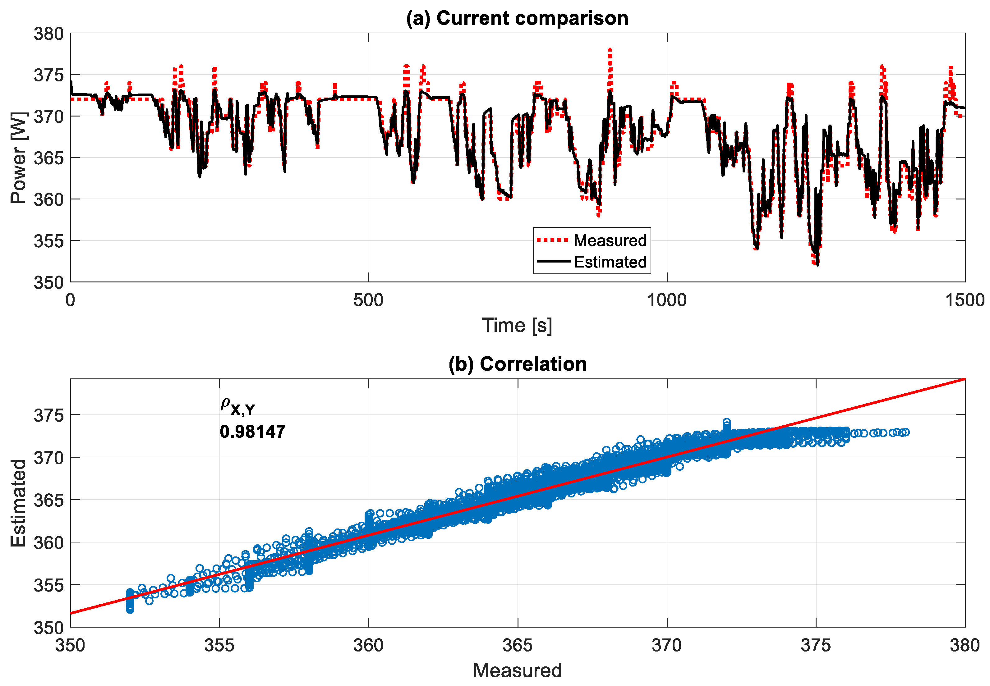
The battery voltage model is already validated in [33]. However, all test maneuvers were performed with relatively low speeds and short testing periods due to the limited area of the testing site. Therefore, the VUT in this work underwent a WLTP class two (WLTP2) driving cycle on a roller dynamometer test bench to validate the model for higher speeds and a more extended test period. Figure 12 displays that the battery model estimated the total battery-pack output voltage, corresponding to the measured battery current, with a high Pearson correlation coefficient (Pearson correlation coefficient—Wikipedia, https://en.wikipedia.org/wiki/Pearson_correlation_coefficient#cite_note-3, accessed on 27 November 2023) of 0.981.

The model did not foresee some spikes since they are caused by the influences of the unpredictable slipping between the tires and the rollers during acceleration and deceleration. This high accuracy is related mainly to the battery model [32]. The battery model must be as realistic as possible because the total energy consumption is be linked directly to the accuracy of both the V_batt and I_batt.

4.2. Validation of the Total Energy Consumption Model

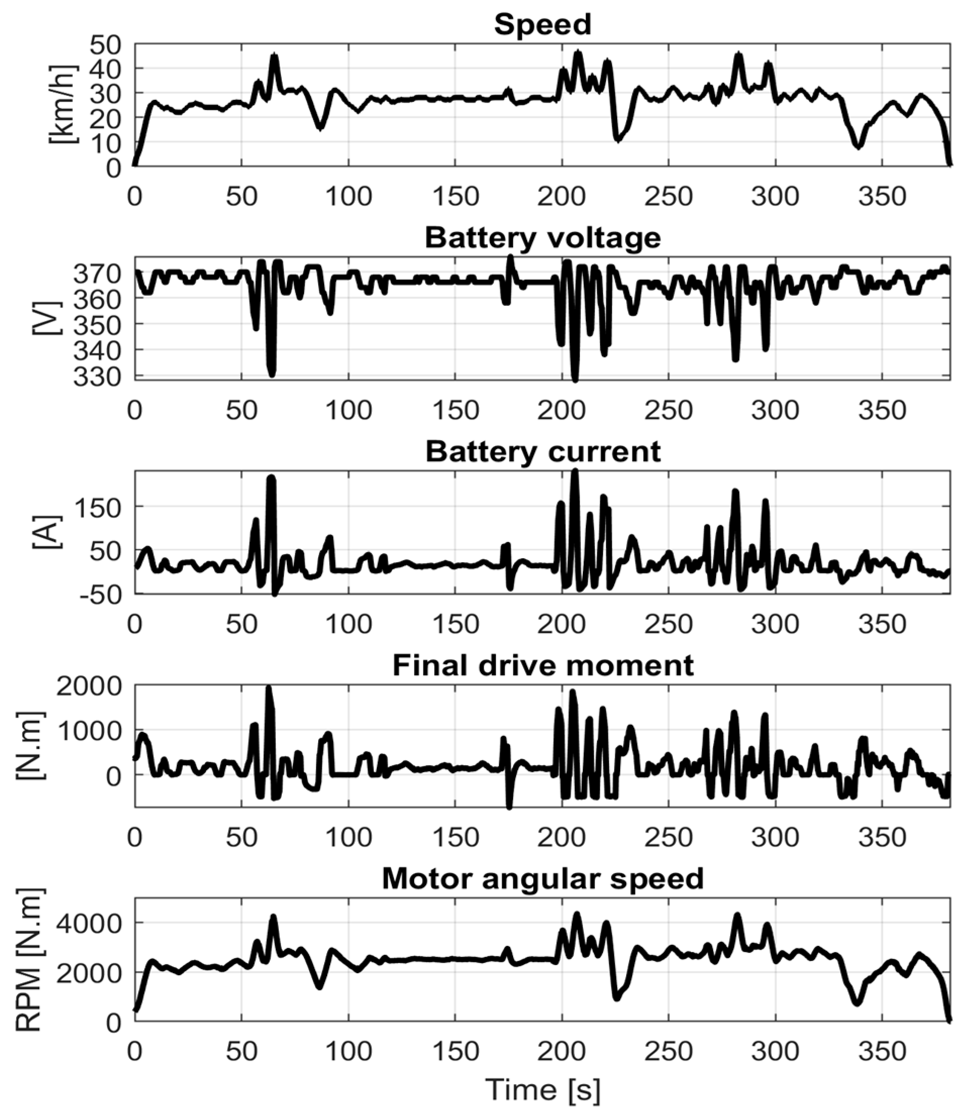
The energy consumption model is validated using the measured data from the measurement of the test vehicle. The validation target is to determine the estimation accuracy of the power transferred through electric vehicles’ powertrain, i.e., the electrical power consumed from the battery and then transformed into mechanical driving power and power losses. The driver applied a dynamic pedal input to create a dynamic maneuver for about 385 s. The test results are displayed in Figure 13.

The positive battery current corresponds to the discharged current during the driving mode, whereas the negative values occur during the braking. Hence, there is no charging for the battery. It can be noticed that the voltage dropped drastically during the high acceleration driving and then remained around 370 V while braking. The final drive moment is produced at the axles after the motor’s torque is transferred through the total gear ratio transmission, responding similarly to the battery current. Finally, the electric motor rotational speed along the test maneuver is also shown. 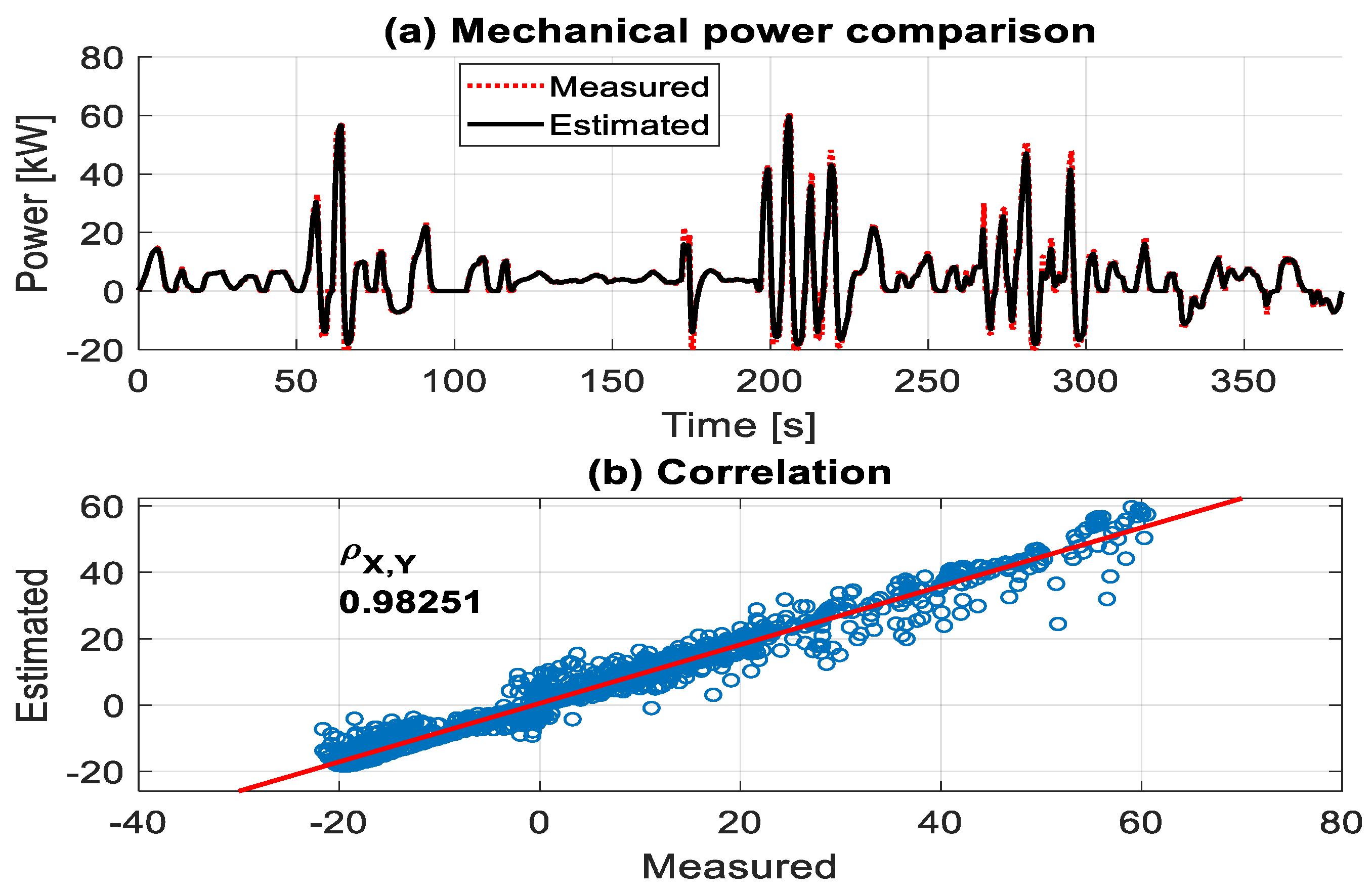Given the measured speed profile, as shown in Figure 11, the VUT simulation model was able to estimate the mechanical power that needs to be delivered by the powertrain to overcome the corresponding driving resistances. The accuracy of P_mech, attained from the multiplication of the estimated angular speed and moment, correlates to 0.983 compared to the expected results, as in Figure 14.

The next step is to estimate the electrical power components, i.e., the V_batt during the maneuver and the withdrawn I_batt from the battery pack. The total P_ins is determined at each instant by adding the mechanical and electrical losses in the powertrain system, as shown in Figure 11. 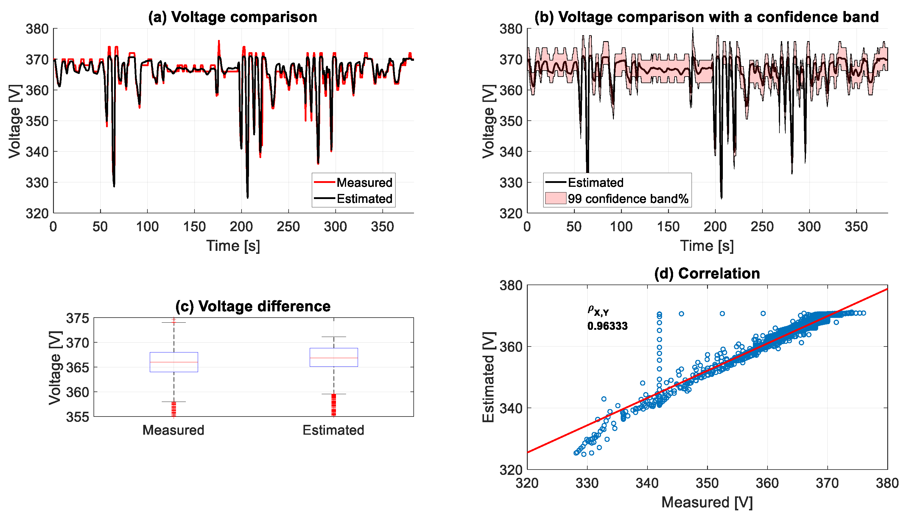The I_batt is then estimated according to Equation (15) at every instant, and is an excellent overall match for P_ins, with a correlation of 0.973, as shown in Figure 15. Due to the low precision of the voltage measurements, as shown in Figure 16a, the correlation of V_batt to the measured voltage has slightly diminished to 0.963, as shown in Figure 16d, even though all the estimated values of V_batt are found within a 99% confidence band compared to the measured battery-pack voltage, as demonstrated in Figure 16b. It can even be noticed from Figure 16c that the mean value of the measured value is 366 V, while V_batt has a mean of 366.84 V, which confirms the high accuracy of the voltage model. 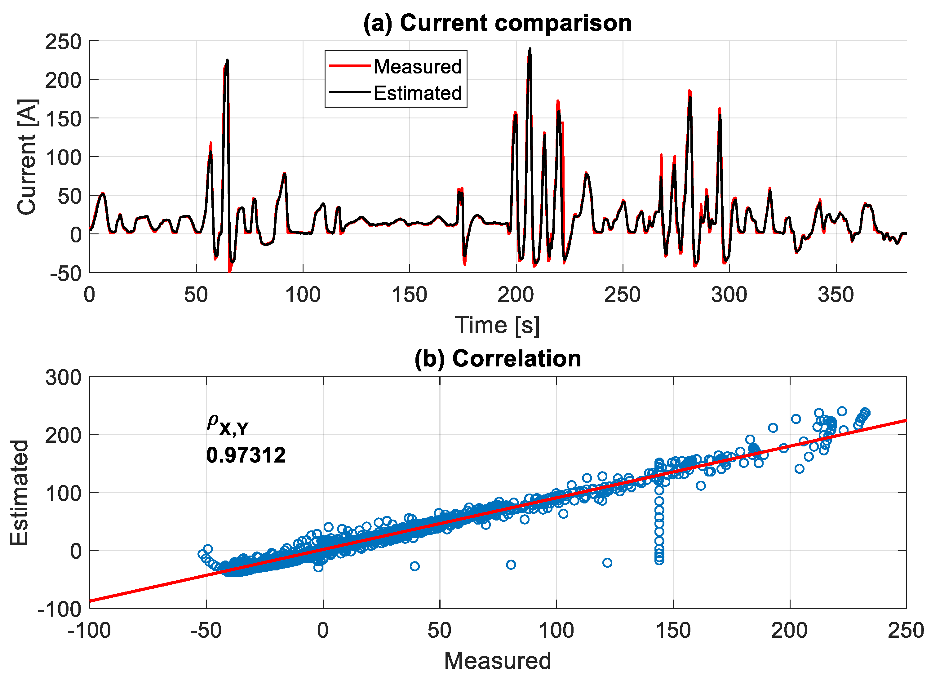Figure 17 reveals that the estimation of I_batt from this complex model is remarkably accurate, with a correlation of 0.973 relative to the measurements. The accuracy of the results is ascribed to the detailed modeling and accurate parametrization, especially for the battery model. Despite the frequent and severe fluctuations of different physical quantities along the measurements, the integrated model of several submodels did not accumulate high errors after this series of calculations.

The most critical quantity that should be measured as accurately as possible in the proposed model is the vehicle’s speed since the whole chain of calculations for the final energy consumption begins with it. If the speed-measured signal was distorted by high noise or the low resolution of speed measurement, the error in energy consumption estimation is expected to increase. A possible solution could be to contain a prediction model for the vehicle’s speed.

5. Conclusions

Many studies focused on creating explicit models to estimate energy consumption for EVs. Several requirements accompany this type of modeling: driving long routes, assuring suitable environmental conditions, and preparing specific measurement instruments. Moreover, the results would be valid for the particular test vehicles; the developed models might not be suitable for other vehicles with different specifications. Other works built physical models of the complete vehicle, but the models must be more detailed to produce the desired energy consumption accuracy. This paper is concerned with creating a generic simulation model for estimating the energy consumption of electric vehicles that is simple to model yet provides highly accurate results. A backward model method is considered in this work for creating the complete electric vehicle since the main objective is estimating the energy consumption based on the vehicle’s speed. Also, no model exists for the interaction between the pedals and the motor through the vehicle control unit. The powertrain model includes a detailed Li-Ion battery model and a generic power loss model for electric vehicles. Furthermore, the model is parameterized according to the technical data of a specific test vehicle. Finally, the proposed powertrain model is incorporated with a vehicle dynamic simulation model to create the complete simulation model for the vehicle under the test. The battery simulation model is validated in two stages. Firstly, the battery voltage (V_batt) estimation is validated, given the measured battery current (I_batt). This step is accomplished by executing the WLTP2 drive cycle while mounting the VUT on a chassis dynamometer. The results proved the outstanding accuracy of the battery voltage estimation. Secondly, the battery current (I_batt) is validated by dividing the computed total instantaneous power (P_ins) by the concurrent battery voltage. This validation is realized with a field driving maneuver. Comparing the measured and estimated physical quantities proves the simulation model’s high reliability. Eventually, the complete integrated model is proven to be beneficial in evaluating the overall energy consumption of electric vehicles and predicting the SOC for a specified real driving course.

This work might be extended in various scopes: For example, developing accurate estimation methods for SOC and P_aux to create a standalone estimation model that can be applied for different routes with known or unknown starting and destination points. Moreover, a detailed regenerative braking model could be combined with prediction methods for driver behavior and driving conditions for real-world roads to estimate the remaining driving range for EVs. Furthermore, the proposed method could be implemented for larger vehicles, such as electric buses. Another research area would be implementing this approach for hybrid vehicles. Systematic parametrization techniques would widen the usability scope of the proposed approach to include different types of electric and fuel-cell vehicles.