How Do Financial Development and Industrial Structure Affect Green Total Factor Energy Efficiency: Evidence from China

Abstract

Improving energy efficiency is vital for addressing climate change and reducing carbon emissions in emerging economies. Financial development (FD) is crucial for economic growth, and its environmental impact and the adjustment of the industrial structure (IND) is a crucial lever in China’s economic transition period. This study explored the relationship between FD, IND, and China’s green total factor productivity (GTFEE) from 2000 to 2020 using the super-efficiency SBM-undesirable model, which estimates China’s GTFEE. The ARDL results suggest that FD and IND enhance GTFEE in the long term, with FD promoting GTFEE by facilitating industrial structure adjustments. The Dumitrescu–Hurlin panel causality tests supported this finding. The QRPD panel quantile regression and heterogeneity analysis revealed significant heterogeneity in the effects. With increasing GTFEE, FD exerts a restraining effect, gradually weakening and transitioning into a promoting effect, while the IND consistently plays a promoting role.

1. Introduction

China has experienced rapid economic growth after initiating economic reforms and liberalization. According to the National Bureau of Statistics, starting at CNY 367.9 billion in 1978, approximately constituting 1.7% of the global economic share, it has currently exceeded the remarkable threshold of CNY one hundred trillion in 2020. Its global economic ratio has risen to approximately 17%, establishing itself as the world’s second-largest economy [1]. Extensive economic growth, substantial utilization of various energy resources, and the exploitation of other natural resources have led to elevated energy consumption, resulting in environmental harm, resource depletion, and the release of carbon emissions [2,3]. According to the “Environmental Performance Index: 2022 Report”, China’s EPI index achieved an overall score of 28.40, positioning it in 160th place out of 180 countries and regions in 2022. At the same time, a poor environment can be detrimental to economic efficiency and public well-being [4]. Consequently, environmentally sustainable policies have turned into a vital foundation for emerging economies [5]. Enhancing energy efficiency is a necessary way for developing countries to diminish carbon emissions and combat climate change in developing nations. China is the same. In addition, because of its environmental friendliness, clean energy has been vigorously developed in recent years in various countries. Developing new energy and promoting the clean and efficient use of traditional energy such as coal is an important support for promoting China’s energy revolution and green and low-carbon development and an important measure to address climate change and promote the construction of ecological civilization. It is also a necessary road for China to achieve the “double carbon” goal and task and fulfill its foreign commitments. Since environmental concerns have emerged as a significant hindrance to China’s sustainable progress, our research integrated environmental constraints when evaluating energy efficiency and used green total factor energy efficiency (hereafter, GTFEE) as the main research indicator.

China’s economy has undergone rapid growth since the 1990s and has nearly completed its full integration into the global market. The gradual development of the financial sector in China has provided the essential economic backing for the nation to achieve its sustainable development goals. Lacking financial backing, China would be unable to attain its sustainable development goals. Financial development is usually defined as the deepening and broadening of the financial system and the improvement of financial markets. It encompasses many aspects, such as the number and size of financial institutions, innovation in financial products and services, the stability and transparency of financial markets, and the effectiveness of financial regulation. “The Fourteenth Five-Year Plan for China’s National Economic and Social Development (2021–2025)” indicates a commitment to further deepen financial reform and enhance financial regulation. Financial development has an impact on energy in three main ways: First, it facilitates capital market activities. A robust financial system enhances stock market activity, enabling investors to purchase energy-efficiency-related equipment at lower prices. This, in turn, enhances environmental efficiency in the long term [6]. Furthermore, it reduces information costs and enhances the returns on investments through heightened capital inflow and production activities, resulting in savings and improved returns. This proves advantageous for capital-intensive initiatives, like environmental protection, fostering enhanced environmental quality [7]. Second, it promotes the technological progress of enterprises. Academics have argued that the financial sector can finance investment in technologies with high energy input–output ratios [8,9]. Financial development and advances in green technology can improve energy efficiency. Ultimately, it is possible to increase the efficiency of energy consumption while adhering to environmental standards [8,10]. Third, it expands financing channels. Financial development is conducive to the expansion of the supply of financial resources and the enrichment and diversification of financial products, providing more financing funds and financing opportunities for renewable energy enterprises, expanding financing channels, and alleviating the role of financing constraints [11]. With the increasing maturity of China’s market economy, financial support for the development of the renewable energy industry has gradually entered the market stage. Innovative financial products, together with traditional financial support, are driving the development of the renewable energy industry. General innovative financial products include green credit, green bonds, green finance, and carbon funds. Taking China as an example, venture capital, international organizations, private equity funds, and policy funds have focused on solving the financing difficulties of some renewable energy industries in China. Since the promulgation and implementation of the “Renewable Energy Law”, the Chinese government has introduced a series of policies to promote the development of renewable energy, such as the government promoting the improvement of the renewable energy subsidy mechanism, and the increase in government-led investment in this field has promoted the development of the renewable energy industry to a certain extent. The existing policy incentives mainly cover price incentives, economic incentives, research and development support, market development, and other incentives. In recent years, China’s green finance has developed vigorously, and a multi-level green financial product and market system, including green credit, green bonds, green insurance, green funds, and green trusts, is being formed. By the end of 2021, China’s domestic and foreign currency green credit balance reached CNY 15.9 trillion, and the outstanding balance of green bonds exceeded CNY 1.1 trillion. Overall, China’s green finance has made a leap forward, achieving a major shift from catching up to leading the world [12].

Being the world’s largest energy consumer, China is in the stage of rapid industrialization. As the globe’s foremost energy consumer, China is in the phase of swift industrialization [13,14]. “The 13th five-year plan of national economic and social development of China (2016–2020)” emphasizes that green development can be achieved by adjusting the industrial structure (hereafter, IND). Therefore, improving the efficiency of green development through industrial restructuring has become a prominent issue in the field of sustainable development. After entering the 21st century, driven by multiple factors such as the upgrading of residents’ consumption, the reform of the financial system, such as the reform of the commercial housing system, and its integration into the global industrial chain through accession to the WTO, China’s economy, under the government’s domination and drive, has moved toward a mode of economic development driven by heavy industry, with urbanization and industrialization taking place side by side and economic development being driven by a large amount of investment. Investment has surpassed consumption as the most important factor driving GDP. The heavy-chemical industry sector, represented by real estate and infrastructure-related sectors, has rapidly developed [15,16], driving the rapid development of industries such as iron and steel, building materials, coal, petroleum, electric power, raw materials, etc. In 2015, marked by supply-side structural reform, China entered into a new round of structural adjustment, shifting from being factor-driven and investment-driven to innovation-driven, with the pursuit of high quality as the main focus. An innovation-driven and service-oriented new development model with the pursuit of high quality replacing the old development model of a heavy industry-driven economy [17,18]. China’s rapid economic development predominantly depends on an industrial structure with high energy consumption and diminished energy efficiency in comparison with the developed world [19]. The “low-end lock-in” of the industrial supply chain and the irrational entrance and exit of industries impede the energy transition [20]. The absence of alignment between the pace of industrial structure enhancement and the development of regional energy infrastructure has resulted in the squandering of resources [21]. Furthermore, energy consumption and carbon emissions in crucial industrial sectors have consistently represented a significant share. There is a demand for more prudent decision making to promote a positive cycle in which a rational industrial structure fosters efficient energy utilization [22]. In turn, enhanced energy efficiency drives industrial reformation and simultaneously enhances environmental standards [23].

Currently, numerous scholars have conducted research on the relationship between finance, the environment, and other factors, unilaterally, and energy efficiency and energy consumption. Although they have drawn many different results and conclusions, there are few studies that have studied the impact of financial development (hereafter, FD) and the industrial structure, together, on GTFEE. Therefore, this paper places FD, IND, and GTFEE in the same research framework using the ARDL model. In the current economic development context, we believe that investigating this issue holds significant practical and theoretical significance.

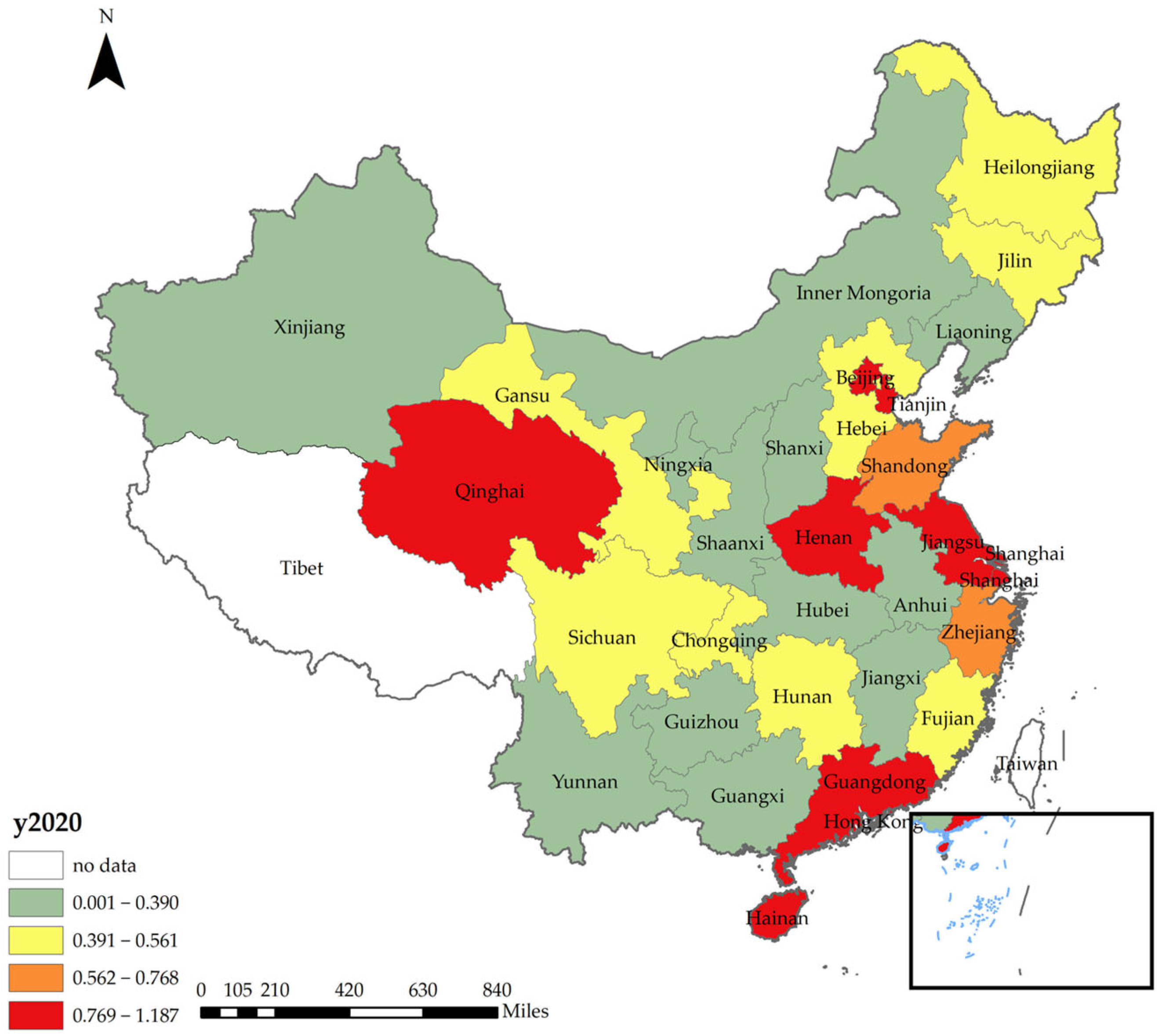
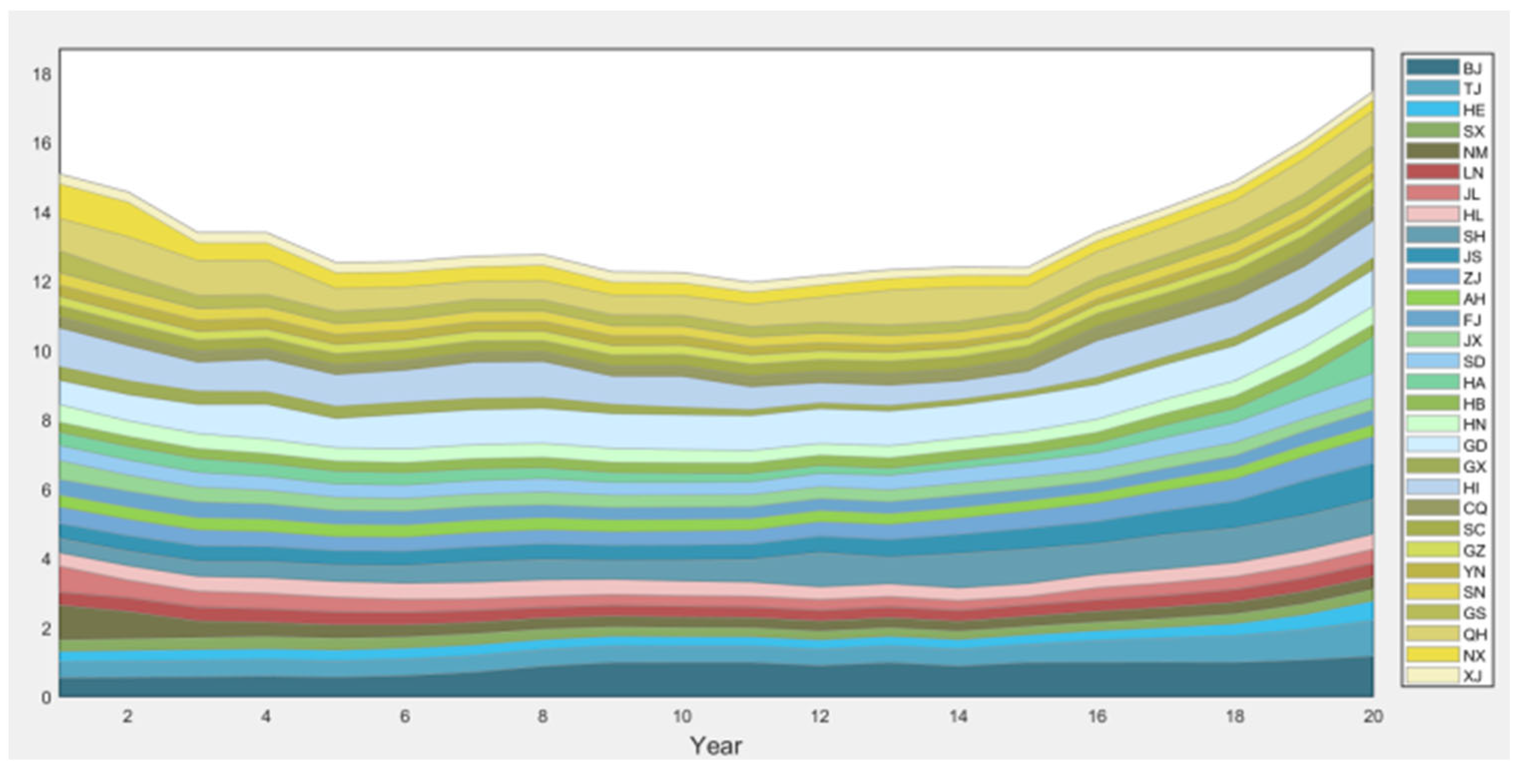
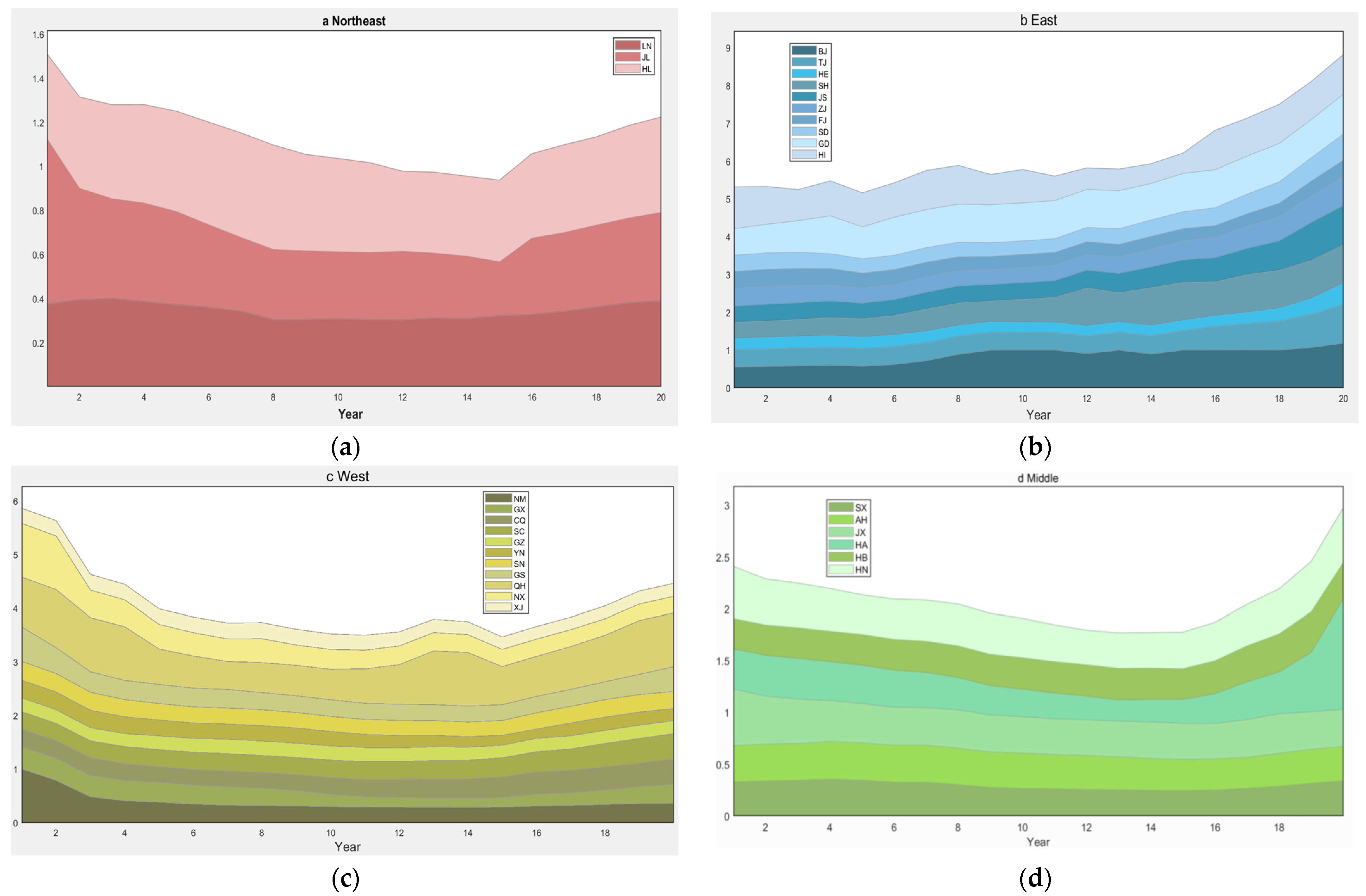
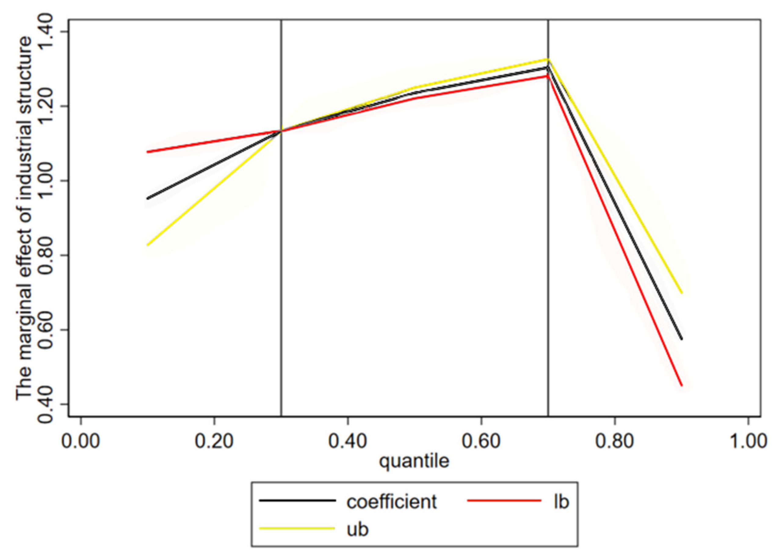
The primary content of this paper is outlined as follows. Firstly, we used the super-efficiency SBM-undesirable model to estimate the GTFEE value for 30 Chinese provinces from 2000 to 2020, taking environmental factors as undesired outputs, so the model measured energy efficiency more comprehensively than the original calculation and described its various distributions. Secondly, for a deeper understanding, this study included financial development and industrial structure in the model and used urbanization, shown as URBAN, government intervention, represented as GOV, and social consumption level, represented as CONSU, as control variables to more comprehensively measure the impacts of explanatory variables on GTFEE. Third, this paper used panel ARDL (PMG/DFE) and CS-ARDL to explore the long-term impacts of FD and IND on GTFEE and then applied Dumitrescu–Hurlin (DH) panel causality tests to determine the interconnections between the three. Finally, in order to analyze heterogeneity and further study the marginal effects of FD and IND under different degrees of GTFEE, this study adopted the QRPD model (quantile regression for panel data with non-additive fixed effects). This method characterized the dynamic evolutionary path of the marginal effects of financial and industrial factors during the progression of energy-oriented sustainable development.

The rest of this document is organized in the following manner. Section 2 provides a succinct review of the current literature. Section 3 evaluates and analyzes China’s GTFEE. Section 4 provides a brief description of the estimation techniques and data used in this study. Section 5 presents and discusses the empirical findings. Finally, in Section 6, conclusions are drawn, and relevant policy implications are discussed.

2. Literature Review

2.1. Measurement of Energy Efficiency

The main measures of energy efficiency include single-factor energy efficiency (SFEE) and total-factor energy efficiency (TFEE). The former is a single-factor indicator, and its common indicator is energy intensity, usually referred to as energy consumption per unit of GDP. Nonetheless, a single factor neglects to account for the influences of other variables on the output. Consequently, the results of TFEE calculations are often biased and increasingly criticized by scholars. TFEE is defined as the optimal ratio of energy inputs to actual inputs required to achieve a given output in best production practice, with other factors of production held constant [24]. Subsequently, TFEE has gained widespread acceptance. Compared with SFEE, TFEE takes into account the effects of interactions between various inputs within the economic framework of energy efficiency. It provides a more precise and objective measure of energy utilization in a region or country.

As the economy develops, scholars have increasingly recognized the significance of environmental protection. Pollution emissions from energy use should be carefully considered when assessing energy efficiency; otherwise, the results may be overstated [25,26]. Certain scholars have incorporated energy use and pollutant emissions into the TFEE structure, thus defining GTFEE [27,28]. When it comes to the specific methods of calculating GTFEE, data envelopment analysis (DEA) is the most widely used method to assess efficiency. The computation results obtained by various researchers reveal that energy efficiency when accounting for both desired and undesired outputs is notably lower than when only contemplating the desired output [29,30,31].

2.2. Related Research on the Impact of Financial Development on GTFEE

On the one hand, the financial sector has been associated with the energy sector in the relevant literature [32]. Financial development directly impacts the efficiency of energy utilization. Financial systems can have an impact on energy consumption by mobilizing savings, generating resources for growth, enhancing business trust, and expanding the scope of the economy [33]. The degree of financial development exhibits a positive correlation with investments in energy and the consumption of energy [34], exerting a significant impact on the energy–growth relationship [35]. On the other hand, financial development has a close connection with green development and environmental concerns. Financial development can offer financial backing for green innovation, reduce information asymmetry, and enhance resource allocation efficiency [36]. The enlargement of the financial sector can facilitate businesses in more efficiently accessing green financial resources at reduced expenses, thereby fostering green business outcomes and aiding companies in expanding their current green business scope while diminishing their dependence on conventional energy sources [37]. Financial structure promotes the advancement of eco-friendly technology innovation, while financial magnitude and effectiveness exert an adverse impact on the innovation of green technologies [38].

Certain scholars contend that the role of financial development does not follow a straightforward positive linear correlation. Instead, they propose a relationship between financial development and energy efficiency that takes the form of an inverted U shape, suggesting a noteworthy influence on energy utilization efficiency only when the degree of financial advancement surpasses a particular threshold [39]. For example, within the context of Saudi Arabia, a non-linear inverted U-shaped correlation is observed between financial development and energy consumption [40]. Financial development has stimulated economic activities in Lebanon, subsequently leading to increased energy consumption [41]. The magnitude of financial institutions (FDS) notably hinders green growth (GG), whereas the extent of stock markets (STO) substantially fosters green growth (GG). A non-linear U-shaped connection is evident between the size of FDS and GG [42]. It is evident that the existing research has either concentrated on the impact of financial development on energy efficiency and consumption or separately explored the connection between financial factors and sustainable development. Limited literature exists that incorporates green factors when examining the influence of financial progress on energy.

This also corresponds to relevant theories on the relationship between economic development and the environment. These include the environmental Kuznets (EKC) hypothesis, suggesting an inverted U-shaped relationship between environmental pollution and economic growth [43,44], which is based on the empirical observation that economic growth is associated with an increase in environmental degradation up to a turning point, after which the quality of the environment begins to improve [45,46]. The emergence of this inflection point leads to an inverted “U”-shaped pattern, which Panayotou called the EKC after the original Kuznets curve [47,48]. Similarly, there is the pollution paradise hypothesis (PPH), which states that firms in pollution-intensive industries tend to build factories in countries or regions with relatively low environmental standards [49,50,51]. The specific transfer and substitution of trade and polluting industries from developed to developing regions in the PPH can also correspond to the declining interval in the environmental Kuznets curve (EKC) [52,53]. There is also the pollution halo hypothesis, Porter hypothesis, and so on [54,55].

2.3. Related Research on the Impact of Industrial Structure on GTFEE

In recent years, with the growing worldwide focus on environmental preservation and sustainable development, the investigation of the influence of the industrial structure on energy utilization has emerged as a prominent subject in the field of economics. Firstly, in a period of worldwide industrial transformation and an expanding energy crisis, alterations in the industrial structure are exerting a more substantial impact on the energy system. Unjustified alterations in structure may hinder the transition of the energy system toward sustainability [56].

The efficiency of industrial energy is closely linked to the inter-sectoral structure [57]. The industrial structure serves as the intermediary between industrial operations and energy efficiency, governing the allocation of production factors and the effectiveness of the conversion between input and output factors [58,59]. Previous research has indicated that the upgrading of the industrial structure, including the shift or relocation of energy-intensive sectors, constitutes a crucial approach for conserving industrial energy and reducing emissions, playing a role in achieving up to 70% of China’s emissions reduction target [60]. The adjustment of the industrial structure is deemed one of the effective methods to achieve sustainable development [61].

However, some scholars contend that there is diversity in how the industrial structure affects GTFEE. The enhancement of energy efficiency is influenced by the industrial structure but displays regional variations [62]. There is a noticeable disparity in energy efficiency between cities, and the impact of the industrial structure on energy efficiency unfolds in a phased pattern [63]. The optimization of an economy’s industrial structure needs to be followed by improvements in productivity and resource efficiency, leading to reductions in carbon emissions and, ultimately, to more environmentally sustainable economic growth [64,65]. Accelerating industrial upgrading and improving the utilization efficiency of energy resources are key measures for curbing carbon emissions in energy-abundant regions [22]. In conclusion, prior research highlights the significance of industrial structure enhancement, particularly the transition away from energy-intensive industries, in accomplishing objectives related to sustainable development. However, it is important to recognize that there are differences in energy efficiency in different regions and that the impact of the industrial structure shows a phased approach.

2.4. Study on the Influences of Financial Development and Industrial Structure on GTFEE

The financial sector is a crucial element of contemporary service industries, and its degree of development is closely linked with industrial structural adjustments. Financial development assumes a catalytic role in resource allocation and the transformation of economic structures [66]. Brown et al. have determined that improvements in the external financing environment for businesses can stimulate technological innovation, while the expansion and liberalization of securities markets can drive technological innovation at the enterprise level, thereby advancing industrial upgrading [67]. Sasidharan et al. conducted a study on the financing environment of industrial enterprises in India from 1991 to 2011 and revealed that financial development has made corporate financing more accessible [68]. This, in turn, has led to increased investments in research and development, thereby fostering corporate growth and structural upgrading. The research also indicated that financial development significantly enhanced the financing environment for infrastructure construction, thereby augmenting the service quality of the communication industry and propelling overall industrial upgrading [69]. In the Chinese context, Lin and Zhao found that as financial development advanced and financial structures improved, the influence of innovation in driving industrial upgrading shifted from being inhibitory to stimulating, following a pattern of marginal increments [70]. Within the constraints of efficiency and financial openness, the influence of innovation on industrial upgrading formed an inverted U-shaped relationship, where innovation initially promoted and later restrained the process. The expansion of the financial sector reduces financing transaction costs and mitigates information asymmetry, directing capital toward strategic emerging industries and new technological sectors [71]. Industrial structural adjustment serves as an efficient pathway to achieve green economic growth by promoting the transfer of factors of production from non-clean industries to clean ones [61]. In terms of spatial aspects, it is concluded that financial development and industrial optimization and upgrading yield positive spatial spillover effects, both contributing to improved resource utilization.

Throughout the domestic and international literature that has been investigated, we can see that scholars have conducted extensive research on the issues of financial development, industrial structure, and energy utilization efficiency. However, the following problems still exist: Firstly, when measuring the index of energy utilization efficiency, although scholars at home and abroad have gradually realized the pollution released by energy utilization into the environment, the undesired output of energy often focuses on a certain aspect of pollution, such as nitrogen oxides or CO₂, which makes it difficult to portray the full picture of the environmental pollution produced by energy utilization. Secondly, logically, there is the possibility that financial development promotes the upgrading of the industrial structure, and changes in the industrial structure have an impact on energy efficiency, but fewer existing studies link the three together and lack the distinction between long-term and short-term impacts. Finally, although scholars at home and abroad have selected specific provinces, economic zones, city clusters, regions, and countries as the objects of study to explore the impact of the direction of financial development and the industrial structure on energy efficiency, the objects and scopes of the studies have been quite broad. However, when taking the whole country as the research object, regional heterogeneity has mostly been taken into account when considering heterogeneity, and the impact of this variable on energy efficiency in China has been studied by region. The analysis of heterogeneity is relatively singular.

Despite being influenced by various factors, it can be argued to some extent that financial development can enhance energy efficiency and promote green development by reducing information asymmetry, lowering financing transaction costs, and fostering green innovation. Additionally, the enlargement of financial magnitude and the enhancement of financial efficiency can facilitate industrial upgrading by improving resource allocation and stimulating innovative vitality. The adjustment of the industrial structure, accompanying technological advancements, though its impact on energy efficiency varies due to regional and temporal differences, remains a crucial factor in achieving sustainable energy development. Logically, there exists the possibility of financial development promoting industrial structural upgrades, which, in turn, affect GTFEE. However, there is currently limited empirical research confirming the relationships between these three factors. Hence, this study aimed to empirically test the impacts of increased financial development and industrial restructuring on energy utilization efficiency.

The main contributions of this paper can be summarized as follows: First, this paper cites a new research indicator, GTFEE, and includes exhaust gas, wastewater, solid waste, and carbon dioxide as undesired outputs when measuring this indicator, thus making the comprehensive evaluation of energy utilization efficiency more comprehensive than the indicators used in previous studies. Especially when clean and renewable natural resources are used for energy production, they emit little to no greenhouse gases or pollutants into the surrounding environment, so the selection of unexpected outputs therefore needs to be as comprehensive as possible to better reflect changes in energy efficiency, which is the point of GTFEE. Second, in terms of research methodology, this paper took the industrial structure as a mediating variable to explore the effects of financial development, the industrial structure, and their interaction terms on GTFEE. Via empirical research, we tested whether the improvement of the financial development level can have an impact on energy efficiency via the adjustment of the industrial structure and analyzed the impact in the long and short terms using the ARDL model. In addition, in terms of research content, this paper also discusses the evolutionary characteristics of the marginal effects of FD and IND using the QRPD model. Thus, it complements existing studies by examining more specifically the heterogeneity of GTFEE across different sub-locations. In conclusion, this study provides empirical evidence supporting the idea that China can harness the complementary advantages of financial development and industrial structural adjustment to promote the green utilization of energy, thereby advancing green development. These research findings not only contribute to theoretical innovations in the development of China’s green economic system but also offer valuable practical insights into China’s economic transformation.

3. Measurement and Analysis of China’s Green Total Factor Energy Efficiency

3.1. Calculation Method for Green Total Factor Energy Efficiency

Farrell initially introduced the concept of “data envelopment analysis” (DEA), a methodology designed for assessing relative efficiency in situations involving multiple inputs and outputs [72]. Nevertheless, within real-world economic production processes, labor, capital, and energy are employed to manufacture industrial goods, and they also give rise to the emission of pollutants, representing undesirable outputs. In contrast with the conventional data envelopment analysis (DEA) model, the SBM (slacks-based measure) that incorporates unanticipated outputs enables the assessment of input and output adjustments, even including undesired outputs. Consequently, the SBM model is closer to actual production conditions and finds extensive application in eco-efficiency and energy efficiency evaluations. Nonetheless, a drawback of the SBM-undesirable model exists in that it does not allow for the decomposition of the efficiency value of the efficient decision-making unit, resulting in the loss of information pertaining to the efficient decision-making unit [4]. Tone introduced an enhanced SBM model for handling undesirable outputs, building upon the foundation of the traditional SBM model [73]. The model combines the advantages of the super-efficiency model and the SBM model and regroups the effective decision units with an efficiency value of one, thus avoiding the loss of information of the effective decision units [74]. The resulting super-efficiency SBM-undesirable model, while considering undesirable outputs, is as follows:

$${\rho }^{*}=\frac{\frac{1}{m}{\displaystyle {\sum }_{i=1}^m\frac{\overline{x}}{x_{i0}}}}{1+\frac{1}{S_1+S_2}({\sum }_{r=1}^{s_1}\frac{s_r^g}{y_{r0}^g}+{\displaystyle {\sum }_{r=1}^{s_2}\frac{s_r^b}{y_{r0}^b}})}$$

(1)

$$s.t.\left\{\begin{array}{l}\overline{x}\ge X\lambda \hfill \\ \overline{y^g}\le Y^g\lambda \hfill \\ \overline{y^b}\ge Y^b\lambda \hfill \\ \overline{x}\ge x_0, \overline{y^g}\le y_0^g, \overline{y^b}\ge y_0^b, \lambda >0\hfill \end{array}\right.$$

(2)

Suppose there are n DMUs, each with input m, desirable output S1, and undesired output S2. The vector form is denoted as $x\in R^m, y^g\in R^{S_1}, y^b\in R^{S_2}$, where $X,Y^g$ and $Y^b$ are matrices, and $X=\left[{\mathrm{x}}_1,x_2\dots x_n\right]\in R^{m\times n}$, $Y^g=\left[y_1^g,y_2^g\dots y_n^g\right]\in R^{S_1\times n}$, and $Y^b=\left[y_1^b,y_2^b\dots y_n^b\right]\in R^{S_2\times n}$. ${\rho }^{*}$ is the efficiency value of the DMU; $n,m$, and $j$ represent the counts of input factors, desirable outputs, and undesirable outputs, and $\lambda$ represents the weight vector. The calculation of GTFEE mainly includes the input, desirable output, and undesirable output. The input variables include capital (K), labor (L), and energy consumption (EU). (1) Capital stock (K): We selected the total fixed asset investment and fixed asset investment price index data and calculated the stock using the “perpetual inventory method” [75]. (2) Labor (L): We used the total number of employees in each province as the labor input [76]. (3) Energy consumption (EU) was measured via the total energy consumption of each province [77,78]. The output indicators were as follows. (1) Desirable output: Real GDP was regarded as the indicator of the desirable output using 2005 constant prices. (2) The undesirable output indicators were as follows: industrial wastewater discharge (WW), industrial waste gas discharge (WG), industrial solid waste generation (WS), and carbon dioxide emissions (CO₂) [79,80]. Specific variables were calculated as shown in

Table 1. China’s energy-saving potential measurement data interpretation.

Variable	Index	Method
Input variable	Capital stock	The continuous inventory method
	Labor	Provincial employment statistics
	Energy consumption	Provincial total energy consumption data
Desirable outputs variable	GDP	Provincial GDP data (constant price in 2005)
Undesirable outputs variable	Wastewater	Discharge of industrial wastewater
	Waste gas	Industrial waste gas emission
	Solid waste	General industrial solid waste
	CO2	Provincial historical end-use energy consumption data *

* IPCC: 2006 IPCC Guidelines for National Greenhouse Gas Inventories^® (Intergovernmental Panel on Climate Change, 2006).

. The selection of these variables was grounded in data collected from national 30 provinces in the period of 2000–2020, sourced from the “China Energy Statistical Yearbook”, “China Statistical Yearbook”, and “China Environmental Statistics Yearbook”.

3.2. Analysis of China’s Green Total Factor Energy Efficiency

3.2.1. Overall Analysis

Using panel data from 30 provinces in China, excluding Tibet, Hong Kong, Macao, and Taiwan, a super-efficiency SBM-undesirable model was constructed to assess China’s GTFEE under environmental constraints from 2000 to 2020. The software used was MATLAB. The calculation values of GTFEE are graphically presented in Figure 1 using an area graph format. In the figure, areas denoted in white pertain to cities that are not included in the sample. The shading of cities with labels signifies their GTFEE levels, with darker colors representing higher GTFEE values. The red areas signify the highest overall GTFEE.

It can be seen that from 2000 to 2020, after a slow decline, China’s GTFEE had gradually increased since 2011 in Figure 2. The initial drop in GTFEE can be linked to the government’s approach during the 12th and 13th Five-Year Plan periods, where the government considered limiting pollutant emissions as a compulsory benchmark, thereby reinforcing the government’s environmental commitment. This has resulted in an improvement in the effectiveness of environmental management. Particularly, the Chinese government has exhibited growing recognition of the significance of low-carbon development, resulting in more conspicuous efficiency improvements.

3.2.2. Regional Analysis

Considering the variations in economic progress and geographical positioning across China, this research classified the 30 provinces into four regions: eastern, central, northeastern, and western. The GTFEE values for these four regions are presented in Figure 3. Generally speaking, the level of GTFEE in the eastern region is significantly higher than that in the west, central, and northeast regions. Moreover, the eastern region’s energy efficiency value shows a positive correlation with time, while the energy efficiency values of the other three regions all fall first, reach their lowest peaks, and then rise. China’s eastern regions and developed eastern coastal provinces mainly focus on the tertiary industry with high output, low energy consumption, and low pollution. The original low-output, high-energy consumption, and high-pollution labor-intensive or capital-intensive industries have been transferred to the central and western regions, thus achieving a balance between economic growth and environmental quality and improving environmental efficiency. Secondly, the rapid economic growth in the eastern coastal areas further produces a large amount of financial funds invested in environmental pollution remediation, which indirectly improves the environmental quality, enhances the level of green technology, and promotes the green total factor productivity. In this way, the eastern provinces not only have a more competitive economic development level than other provinces but also have more advantages in environmental protection and pollution control.

Due to geographical factors, it is difficult for the western region to develop high-efficiency and low-pollution industries, the level of industrialization is slow, and the level of economic development is far lower than that in the eastern region. Many industries that have been eliminated in the eastern part of the country have been transferred to the western part of the country, which makes it more difficult to increase the total factor energy efficiency level in the western part of the country. In recent years, due to the extensive implementation of the “Western Development” strategy in the western region, the industrial structure of the western region has been gradually optimized, the industrialization level has been accelerated, and the energy efficiency has been improved.

The central region is a traditional energy and labor province, so the costs of labor and raw materials are very low, so it has moved a lot of industries that have been eliminated in the east, and this traditional heavy industry, although it brings a considerable degree of economic benefits, has caused an increase in energy consumption, carbon emissions, and other factors that pollute the environment, and the damage caused by rapid economic development exceeds the carrying capacity of the environment, which has led to a decrease in GTFEE. In recent years, the GTFEE value has increased due to the role played by the national “Rise of the Central Plains” strategy and the fact that with the development of the eastern region, the central region has absorbed the industrial development mode and production management experience of the eastern region.

The GTFEE value of the northeast region is the lowest among the four regions. This is because the northeast region is the old industrial base of China, and the northeast is constrained by the industrial structure and the solidification of industrial development in previous years, which has made the economic development in recent years not so optimistic, and the northeast is gradually changing its development mode, but it still needs a process. Based on the layout of the national “Northeast Revitalization” strategy in recent years, the capital investment in the northeast region has increased, resulting in an increase in the GTFEE value of the northeast region between 2016 and 2020.

4. Method and Data

4.1. Model Setting

4.1.1. Panel ARDL Model

In order to investigate the short- and long-term relationships between GTFEE, financial development, and the industrial structure, this study employed the panel ARDL (autoregressive distributed lag) approach introduced by Pesaran et al. [81]. The panel ARDL model is represented as follows:

$${\mathrm{GTFEE}}_{i,t}={\gamma }_i+{\displaystyle \sum _{j=1}^{p_g}{\lambda }_{i,j}{\mathrm{GTFEE}}_{i,t-j}}+{\displaystyle \sum _{j=0}^{p_z}{\delta }_{i,j}}{Z}_{i,t-j}+{\epsilon }_{i,t}$$

(3)

$$\mathrm{Where} Z_{i,t}=({\mathrm{FD}}_{i,t}),({\mathrm{IND}}_{i,t}),({\mathrm{GOV}}_{i,t}),({\mathrm{SCL}}_{i,t})$$

(4)

Furthermore, the speed at which the system adjusts to the long-term equilibrium after short-term disturbances can be determined using an error correction model (ECM). The ARDL approach was employed in the ECM format as follows:

$$\Delta {\mathrm{GTFEE}}_{i,t}={\eta }_i+{\phi }_{{}_i}({\mathrm{GTFEE}}_{i,t-j}-{\theta }_{0,i}-{\theta }_i{Z}_{i,t}){\displaystyle \sum _{j=1}^{p_g-1}{\lambda }_{i,j}{}^{*}}\Delta {\mathrm{GTFEE}}_{i,t-j}+{\displaystyle \sum _{j=0}^{p_z-1}{\delta }_{i,j}{}^{*}}\Delta Z_{i,t-j}+{\zeta }_{i,t}$$

(5)

where $i$ = 1,2,…,N denotes the cross-sectional units, $t$ = 1,2,…,T denotes the time (annual) periods, $j$ is the number of time lags, $p$ is the variables’ lag, $Z_{i,t}$ denotes the vector of variables, and ${\phi }_{{}_i}$ is the impact of the error correction mechanism. ${\gamma }_i$(${\eta }_i$) is the group effect, ${\epsilon }_{i,t}$(${\zeta }_{i,t}$) is the error term, and the rest of the coefficients correspond to the short-term coefficients. We calculated Equation (2) with both the dynamic fixed effects (DFE) and the pooled mean group (PMG) estimators. With the exception of the intercept, the DFE estimator assumes that the parameters in all parts of the panel are homogeneous. The PMG estimator permits the short-run parameters to vary by state but enforces homogeneity for the long-term ones. The ARDL model is used to simultaneously address both short-run and long-run co-integrated variables. This approach offers advantages over other conventional multivariate cointegration methods, as it effectively mitigates the endogeneity problem.

4.1.2. Cross-Sectionally Augmented ARDL Model

The cross-sectionally augmented ARDL model builds on individual estimates involving the lagged dependent variable and the lagged cross-sectional mean while taking into account cross-sectional dependencies [82]. The cross-sectionally augmented ARDL model permits estimations of mean groups with heterogeneous slope coefficients [83]. The inclusion of lagged cross-sectional averages is particularly effective in preventing endogeneity problems. Consequently, the CS-ARDL model possesses the capability to handle cross-dependence (CD) and the heterogeneity of slopes. In conjunction with the considerations mentioned above, we chose CS-ARDL for further empirical analysis. The CS-ARDL estimation regression is as follows:

$${\mathrm{GTFEE}}_{i,t}={\alpha }_i+{\displaystyle \sum _{j=1}^{p_g}{\mu }_{i,j}}{\mathrm{GTFEE}}_{i,t-j}+{\displaystyle \sum _{j=0}^{p_z}{\beta }_{i,j}}{Z}_{i,t-j}+{\displaystyle \sum _{j=0}^{p_m}{\varphi }^{\prime }{}_{i,j}}{\overline{M}}_{i,t-j}+{\epsilon }_{i,t}$$

(6)

In Equation (4), the average of all of the variables is represented by ${\overline{M}}_{i,t-j}=({\overline{GTFEE}}_{i,t-j},{\overline{Z}}_{i,t-j})$, and $p_g$, $p_z$, and $p_m$ denote the lagged variables. The long-run coefficient estimate for the average group is:

$${\widehat{\pi }}_{CS-ARDL,i}=\frac{{\displaystyle {\sum }_{j=0}^{p_z}{\widehat{\beta }}_{i,j}}}{1-{\displaystyle {\sum }_{j=0}^{p_g}{\widehat{\mu }}_{i,j}}}$$

(7)

The mean group is illustrated as:

$${\widehat{\pi }}_{MG}=\frac{1}{N}{\displaystyle \sum _{i=1}^N{\widehat{\pi }}_i}$$

(8)

where ${\widehat{\pi }}_i$ denotes the individual estimations of each cross-section. The error correction form of the CS-ARDL method is given with:

$$\Delta {\mathrm{GTFEE}}_{i,t}={\alpha }_i+{\nu }_i\left[{\mathrm{GTFEE}}_{i,t-j}-{\widehat{\pi }}_i{Z}_{i,t}\right]+{\displaystyle \sum _{j=1}^{p_{{}_g-1}}{\mu }_{i,j}{}^{*}\Delta }{\mathrm{GTFEE}}_{i,t-j}+{\displaystyle \sum _{j=0}^{p_z}{\beta }_{i,j}{}^{*}}\Delta Z_{i,t-j}+{\displaystyle \sum _{j=0}^{p_m}{\varphi }_{i,j}^{\prime }{}^{*}}{\overline{M}}_{i,t-j}+{\epsilon }_{i,t}$$

(9)

where ${\nu }_i$ indicates the adjustment speed of the error correction.

4.1.3. Panel Causality Test

With the regression findings of the ARDL model, this study could deduce the short- and long-term connections between FD, IND, and GTFEE. Nevertheless, the direction of the causal link between these three variables remained uncertain. Hence, this paper employed the Dumitrescu–Hurlin panel causality test, derived from the Granger causality test, to scrutinize the causal associations between these three variables [84]. The specific model is expressed as follows:

$$y_{i,t}={\eta }_i+{\displaystyle \sum _{k=1}^K{\omega }_{i,k}{y}_{i,t-k}}+{\displaystyle \sum _{k=1}^K{\rho }_{i,k}}{x}_{i,t-k}+{\epsilon }_{i,t}$$

(10)

where both $y$ and $x$ refer to GTFEE, FD, and IND; $k$ stands for the lagging length; ${\delta }_{i,k}$ is the regression coefficient that accounts for differences between the cross-sections; ${\omega }_{i,k}$ denotes the autoregressive coefficient; and $y_{i,t}$ and $x_{i,t}$ are two smooth series of observations at individual $i$ and time $t$. The DH panel causality test allows the regression coefficients to be variable for each cross-section (i.e., the coefficients differ between individuals at the same time).

4.1.4. Quantile Regression for Panel Data

In order to investigate the evolutionary characteristics and heterogeneous effects of the roles played by FD and IND in different developmental stages of GTFEE, a quantile regression panel data (QRPD) model was used in this study. The QRPD model is a specific example of the generalized quantile regression (GQR) model [85]. In this paper, the adaptive Monte Carlo method (adaptive MCMC) was chosen to estimate the QRPD model [86]. QRPD introduces the panel quantile estimation into the instrumental variables approach framework so that the random disturbance term contains the fixed effects and ensures the indivisibility of the random disturbance term. Therefore, the QRPD model has the advantage of estimating the coefficients more accurately, and the estimation results are more robust than those using traditional panel quantitative models [87]. This paper selected five quartiles (10%, 30%, 50%, 70%, and 90%) to construct QRPD’s panel quantile function:

$$Q_{{\mathrm{GTFEE}}_{i,t}}={\sigma }_1(\tau ){\mathrm{FD}}_{i,t}+{\sigma }_2(\tau ){\mathrm{IND}}_{i,t}+\eta (\tau )X_{i,t}$$

(11)

where $\tau$ denotes the corresponding quantile; $Q_{GTFE{E}_{{}_{i,t}}}$ refers to the GTFEE development under the corresponding quantile; $F{D}_{i,t}$ denotes the financial development under the corresponding quantile; $IN{D}_{i,t}$ denotes the industrial structure under the corresponding quantile; and $X_{i,t}$ denotes a series of control variables.

4.2. Variables and Data

4.2.1. Dependent Variable

The traditional TFEE measurement does not account for unexpected outputs, consequently resulting in an overestimation of the actual energy efficiency. This inaccuracy can lead to errors in the assessment of changes in economic performance and social welfare. Therefore, this paper used the super-efficiency SBM-undesirable model to estimate the GTFEE in China (the detailed calculation procedure and results are presented in the Section 3).

4.2.2. Independent Variables

We had two independent variables: financial development (FD) and industrial structure (IND). Financial development was measured as the ratio of the year-end deposit and loan balances of financial institutions to GDP [88]. Then, this paper adopted the entropy value method to calculate the comprehensive index of industrial structure, which included four sub-indicators. (1) The Theil index was utilized to evaluate industrial structure optimization (ISO), which represents the balanced level of growth in all segments of the industry. (2) Industrial structure upgrading (ISU) was measured via the ratio of the value added of the tertiary sector to that of the secondary sector [89]. (3) The ratio of the value added of the tertiary industry to the regional GDP was used to indicate the proportion of the output value of the tertiary industry. (4) The ratio of technology market turnover to the regional GDP was employed as a measure for the marketization of technological achievements.

4.2.3. Control Variables

To avoid the problem of omitted variable bias, we used multiple control variables. The level of social consumption (hereafter, SCL) was expressed as the ratio of the total retail sales of consumer goods to the provincial GDP in each province [90]. An increase in the level of national income promotes the expansion of the consumption scale and an increase in the level of consumption, which, in turn, leads to changes in the resource consumption intensity and ecological environmental pressure, such as domestic garbage and automobile exhaust, which are all consumption-type pollution. The ratio of the urban population to the total population was used to measure the level of urbanization (hereafter, URBAN) [91]. Urban expansion not only increases vehicle emissions but also increases energy consumption, damaging the ecological environment [92]. Government intervention (hereafter, GOV) was expressed in terms of fiscal expenditure as a percentage of regional GDP.

4.2.4. Data Sources

This study utilized panel data covering the period from 2000 to 2020 for 30 provinces in China. Notably, data for Taiwan, Macau, Hong Kong, and the Tibet Autonomous Region of China were conspicuously absent and, therefore, were excluded from the analysis. The data used in this article primarily originate from the “China Energy Statistics Yearbook”, “China Statistical Yearbook”, “China Financial Statistics Yearbook”, and “Wind Information Database”. This study standardized the nominal data using 2005 as the base period to ensure comparability. This study used linear interpolation to fill in the data for missing statistical indicators for some years. Additionally, MATLAB 2016 was used to implement the super-efficiency SBM model. Stata 16.0 was used for all other analyses.

Table 2. The statistical description of variables.

Variable	Definition	Obs.	Mean	Std. Dev.	Min.	Max.
GTFEE	Green total factor energy efficiency	630	0.453	0.231	0.172	1.187
FD	Financial development	630	2.910	1.055	1.413	7.578
IND	Industrial structure	630	0.0969	0.0784	0.0439	0.691
URBAN	Urbanization	630	0.512	0.153	0.196	0.896
SCL	The level of social consumption	630	0.361	0.0626	0.218	0.582
GOV	Government intervention	630	0.207	0.0964	0.0689	0.643

presents a summary of the descriptive statistics for the variables used in this research.

5. Empirical Results and Discussion

5.1. Panel Unit Root Test Results

Before applying panel cointegration tests, it was essential to ensure the stationarity of the variables used in this study. Non-stationary data often result in spurious regression outcomes. Given that the panel data for the provinces may show correlations due to some joint effects, a cross-sectional correlation test was conducted. The second-generation unit root test was used to test variables with cross-sectional correlations. These tests included the Pesaran CIPS test and the cross-sectionally augmented Dickey–Fuller (CADF) test as described by Pesaran in 2007 [93].

Table 3. Results of panel unit root tests.

Variable	Pesaran CD	CIPS	CADF
GTFEE	20.764 ***	−2.130	−1.552
ΔGTFEE		−3.082 ***	−2.266 ***
FD	79.779 ***	−1.495	−1.661
ΔFD		−3.181 ***	−2.017 *
IND	64.971 ***	−2.266	−1.673
ΔIND		−3.677 ***	−2.399 ***
URBAN	91.982 ***	−1.694	−2.335 ***
ΔURBAN		−4.055 ***	−2.672 ***
SCL	34.409 ***	−2.868 ***	−1.947
ΔSCL		−4.240 ***	−2.731 ***
GOV	83.079 ***	−2.133	−1.325
ΔGOV		−3.375 ***	−2.664 ***

Notes: *, and *** indicate statistical significance at 10%, and 1%, respectively.

presents the results of the panel unit root test. Clearly, most of the data series were non-stationary at level I(0), but all variables became stationary at the first difference I(1).

5.2. Panel Cointegration Regression

The conventional cointegration test proposed by Pedroni in 1999 and Westerlund in 2007 was used in this study to assess the dynamic short- and long-run relationships between these variables [94,95].

Table 4. Results of panel cointegration tests.

Tests		Stats.	Prob.
Pedroni test	Alternative hypothesis: common AR coefs. (within-dimension)
	Panel v-Statistic	−1.207	0.886
	Panel rho-Statistic	4.428	1.000
	Panel PP-Statistic	−3.520	0.0002
	Panel ADF-Statistic	−2.909	0.0018
	Alternative hypothesis: individual AR coefs. (between-dimension)
	Group rho-Statistic	7.406	1.000
	Group PP-Statistic	−2.368	0.0089
	Group ADF-Statistic	−4.143	0.000
KAO test	ADF	−3.674	0.0001

and

Table 5. Results of Westerlund cointegration test.

Statistic	Gt	Ga	Pt	Pa
Value	−3.037	−7.361	−23.878	−12.723
p-value	0.012 **	1.000	0.000 ***	0.177

Notes: **, and *** indicate statistical significance at 5%, and 1%, respectively.

present the results of the panel cointegration tests. The null hypothesis of the Pedroni cointegration test was rejected at a 1% level of significance for both the PP statistic and ADF statistic values. In addition, the test statistics of the ADF test in conjunction with the Kao cointegration test demonstrate statistical significance at the 1% level. The Westerlund test allows for cross-sectional dependency and heterogeneous slopes when estimating an equilibrium relationship [96]. The outcomes presented in Table 5 indicate that there is a significant cointegration relationship for all the relevant variables, as affirmed by both panel and group statistics. Therefore, the outcomes of the panel cointegration test validate the enduring correlation between GTFEE and both financial development and the industrial structure.

5.3. Slope Homogeneity Test

In the estimation of panel data, this paper used the slope homogeneity test to verify whether the variables were heterogeneous. The test posits that all the slope coefficients are uniform. The results of this test are detailed in

Table 6. Results of slope homogeneity test.

Test	Value	p-Value
$\widehat{\Delta }$	12.534	0.000 ***
$\widehat{\widehat{\Delta }}$	15.931	0.000 ***

Notes: *** indicates statistical significance at 1%.

, indicating the presence of heterogeneity among the variables. Therefore, we used quantile regression to further analyze the heterogeneous effects of FD and IND on the impact of GTFEE.

5.4. ARDL Regression Analysis

This analysis proceeded to examine the relationships between FD and IND in relation to GTFEE via the application of pooled grouped mean (PMG-ARDL), as proposed by Pesaran and Shin, and common correlated effects estimation, commonly referred to as CS-ARDL, following the methodology introduced by Chudik and Pesaran. In addition, this study also estimated the panel ARDL model using the dynamic fixed effects (DFE) estimator. The results of the empirical estimation are shown in

Table 7. Results of panel ARDL regression.

		(1) PMG	(2) DFE	CS-ARDL	CS-ARDL
Long-run coefficients	FD	0.203 ***	0.092 *	0.017 *	0.016 **
	IND	1.009 ***	1.479 ***	0.103 **	0.645 **
	SCL	−2.189 ***	−0.280 **	0.141	−1.229 **
	GOV	−1.807 ***	−0.730	0.347 *	0.452
	URBAN	1.479 ***	0.977 **	0.714 *	0.535 *
	FD × IND				0.328 **
Error correction coefficients	ECT (−1)	−0.130 **	−0.209 ***	−0.157 ***	−0.106 ***
Short-run coefficients	D(GTFEE(−1))	0.178	0.065 *	−0.031	−0.057 **
	D(FD)	−0.017	−0.012	0.064 **	−0.041
	D(FD(−1))	−0.027 *	−0.028*
	D(IND)	0.558	−0.189	−0.164	−0.725
	D(IND(−1))	−0.489	−0.041
	D(SCL)	−0.317	−0.072	−0.210	−0.288
	D(SCL(−1))	−0.017	−0.111
	D(GOV)	−0.276	0.042	0.292	0.272
	D(GOV(−1))	0.257	0.425 **
	D(URBAN)	−0.797	−0.388	−0.994	0.588
	D(URBAN(−1))	−0.014	0.024
	D(FD × IND)				0.587 *
	Constant	0.024	−0.039	0.019	0.024

Notes: *, **, and *** indicate statistical significance at 10%, 5%, and 1%, respectively. The number of lags is based on the Akaike information criterion (AIC).

, containing columns (1) and (2) for panel ARDL and columns (3) and (4) for CS-ARDL. Notably, columns (3) and (4) report the moderating effect of FD on IND, respectively, containing the interaction term FD × IND.

The significant negative value of ECT (−1) in Table 7 suggests that there is a long-run relationship between FD and IND, and GTFEE in China. Therefore, the coefficient must be negative in statistical significance. The results imply that the rate of imbalance correction varies from 10.6% to 20.9% in a year and is statistically significant at 1%, except for in col (1).

In terms of the long-term relationship, the findings show that China’s FD and IND have a significant positive impact on GTFEE. Specifically speaking, this study shows that the relationship between FD and GTFEE is statistically positive in all four model estimations, for example, the coefficient in col (1) is 0.203, the coefficient in col (2) is 0.092, the coefficient in col (3) is 0.017, and the coefficient in col (4) is 0.016. These findings are consistent with those of many studies. Köksal et al. propose that the level of efficiency in the financial system has a positive correlation with the scale of investments in energy efficiency and renewable energy in each country [97]. Financial development enhances the accessibility of investment capital, facilitating businesses’ access to the necessary funds for the development and adoption of green technologies and sustainable development [98]. Consequently, this fosters increased investments in renewable energy, energy efficiency, and various environmentally friendly initiatives [99]. Hence, efficient energy serves as a solution for achieving sustainable growth [100].

In summary, the improvement of GTFEE can be attributed to two aspects. Firstly, it is manifested in an increase in energy utilization efficiency, leading to a higher expected output under constant input variables. Secondly, it can be attributed to the increased utilization of clean and renewable energy sources, resulting in a significant reduction in undesired outputs, particularly in terms of CO₂ emissions, while maintaining the same level of expected output. Similarly, the role of industry structure in influencing GTFEE can be reflected in these two aspects.

This study revealed a statistically significant positive correlation between IND and GTFEE in all empirical evaluations, for example, the coefficient in col (1) is 1.009, the coefficient in col (2) is 1.479, the coefficient in col (3) is 0.103, and the coefficient in col (4) is 0.645. More specifically, every 10% increase in the industrial structure can increase GTFEE by 1.03~14.79%. Industrial restructuring is closely intertwined with changes in energy structure [101]. It also contributes to optimizing energy structure and achieving a balance in supply and demand [102]. In the past, the development of China’s extensive economic development heavily relied on the consumption of energy resources, with the rate of energy resource consumption even exceeding the speed of economic growth, resulting in low energy resource efficiency. This development model has given rise to a large number of energy-intensive industries, most of which are industrial. With green development in recent years, China’s industrial structure has been continuously transformed and upgraded, and the proportions of industries, especially heavy industry, in the economic structure will continue to decline, and some high-energy-consuming industries have been phased out. This industrial structural upgrade, driven by technological innovation, contributes to enhancing production quality and efficiency, thereby contributing to reducing energy intensity and improving energy efficiency.

The effect of FD on GTFEE can be mediated via the mediator IND. The coefficient of the interaction term FD × IND is statistically positive (with a coefficient of 0.328) in the CS-ARDL estimation. This implies that financial development can improve the financial environment and promote industrial upgrading, thus promoting industrial activities and optimizing the industrial structure over time. This, in turn, affects the quality of the environment and boosts energy utilization efficiency. Therefore, in the pursuit of low-carbon sustainable development, optimizing capital allocation via FD plays a crucial role in fostering the improvement of IND. It is essential to acknowledge that the connections between short-term variables may vary from those observed in the long term. The impacts of FD and IND on GTFEE remain uncertain, and the results may not necessarily be statistically significant.

5.5. Dumitrescu–Hurlin Panel Causality Tests

This paper utilized the Dumitrescu and Hurlin non-causality test to explore the short-term dynamics among the variables [84]. In essence, this empirical analysis aimed to determine the direction of short-term dynamic panel causality between variables by employing a model that accounted for the heterogeneity across the cross-sections. The results of the estimation of short-term causality are shown in

Table 8. Results of Dumitrescu–Hurlin panel causality tests.

Null Hypothesis:	W-Stat.	Zbar-Stat.	Prob.	Remarks
FD←≠→GTFEE	6.6599	4.1824	0.0800	Unidirectional causality: FD→GTFEE
GTFEE←≠→FD	4.7889	1.5681	0.4400
IND←≠→GTFEE	10.1566	9.0685	0.0030	Unidirectional causality: IND→GTFEE
GTFEE←≠→IND	6.3425	3.7389	0.1020
FD←≠→IND	7.5344	5.4044	0.0130	Unidirectional causality: FD→IND
IND←≠→FD	6.4709	3.9184	0.1290	Unidirectional causality: FD→GTFEE

.

This study’s findings reveal unidirectional causality, with causation running from financial development to GTFEE (FD/GTFEE), industrial structure to GTFEE (IND/GTFEE), and financial development to industrial structure (FD/IND). Sasidharan et al. also came to a similar conclusion that the optimization of financial development can positively contribute to the industrial structure [68]. These results display that the growth of FD and IND both have an impact on GTFEE. The single causal relationship between FD and IND means that financial development can affect GTFEE by promoting the adjustment of the industrial structure. Importantly, the absence of a bidirectional causal relationship between the variables suggests that the estimates are also robust in terms of endogeneity bias.

5.6. Heterogeneity Regression Results

5.6.1. Panel Quantile Regression Results

In order to study whether the impact of GTFEE on FD and IND is heterogeneous at the GTFEE level in different provinces, we applied the QRPD regression proposed by Powell [85]. Using quantile regression, the influences of FD and IND on GTFEE under a conditional distribution could be estimated. The dynamic evolution trajectory with special attention to marginal effects could also be obtained.

Table 9. Results of panel quantile regression.

	10th	30th	50th	70th	90th
IND	0.9527 ***	1.1337 ***	1.2355 ***	1.3039 ***	0.5752 ***
	(12.5975)	(2.1 × 103)	(140.5157)	(94.8114)	(7.6204)
FD	−0.0052 ***	−0.0036 ***	0.0027 ***	0.0335 ***	0.0114 ***
	(−3.1951)	(−45.4927)	(3.7738)	(27.0595)	(4.7796)
GOV	−0.3137 ***	−0.5238 ***	−0.4201 ***	−0.2598 ***	−0.3860 ***
	(−24.7771)	(−5.3 × 102)	(−1.1 × 102)	(−1.0 × 102)	(−23.1459)
URBAN	0.1097 *	0.1726 ***	0.1589 ***	0.1983 ***	1.1050 ***
	(1.6476)	(423.0294)	(38.8661)	(21.1159)	(20.6115)
SCL	−0.0356	−0.1644 ***	−0.4264 ***	−0.7143 ***	−2.3287 ***
	(−0.9071)	(−2.6 × 102)	(−48.2335)	(−78.2814)	(−49.4184)

Notes: t-statistics in parentheses. *, and *** indicate statistical significance at 10%, and 1%, respectively.

reports the results of the conditional GTFEE distribution.

In the case of financial development, we found the response of GTFEE to FD to be clearly heterogeneous across different quintiles. In other words, the impacts were different under different energy use efficiency distributions. As shown in Figure 4, firstly, when GTFEE was in the lower quintile, with the improvement of efficiency, the inhibition effect of FD on GTFEE was weakened. This result is consistent with the findings that the effectiveness of financial growth for ecologically friendly progress in Belt and Road countries had adverse effects on financial scale, financial deepening, and financial performance during the sampling period in [103]. This negative link can be explained by an underdeveloped financial sector. For example, higher financial costs discourage investment in renewable energy infrastructure and technologies. Secondly, when GTFEE was in the upper quintile, as the efficiency increased, FD had a promoting effect on GTFEE. The promoting effect first increased and then decreased. When the energy efficiency was in the lower quintile, the effect was inhibitory, and when the energy efficiency was in the upper quintile, the effect was promotional. This indicates that the effect of FD on GTFEE reduction is greater in provinces with high energy efficiency than in provinces with low energy efficiency.

As shown in Figure 5, when the energy efficiency was in the lower percentile, the improvement in efficiency enhanced the promoting effect of IND on GTFEE. Conversely, when GTFEE was in the upper percentile, the promoting effect of IND on GTFEE increased initially and then diminished with further efficiency improvements. Secondly, the rise in percentile levels indicates that the impact of IND on the green utilization efficiency of energy has been positive. This result is in line with the findings of most scholars, who hold the view that changes in the industrial structure benefit the energy system [104]. Optimizing the industrial structure requires higher productivity and more efficient use of resources. This, in turn, can reduce carbon emissions and promote greener economic growth. The effective harnessing of energy resources and the refinement of China’s industrial configuration are essential for attaining superior economic growth and ecological equilibrium [105].

5.6.2. Panel PMG-ARDL Heterogeneity Regression Results

Finally, to analyze the heterogeneity in depth, we also employed the panel ARDL model to examine the relationships between GTFEE, financial development, and the industrial structure in China under different degrees of financial development. The results of PMG-ARDL are reported in

Table 10. Results of ARDL.

		FD1	FD2
Long-run coefficients	FD	0.0740 ***	0.00249
	IND	−0.566 ***	1.471 ***
	SCL	0.410 ***	−0.270 ***
	GOV	−0.532 ***	−1.365 *
	URBAN	−0.731 ***	0.453 ***
Error correction coefficients	ECT (−1)	−0.137 ***	−0.205 ***
Short-run coefficients	D(GTFEE(−1))	0.0320	0.0457
	D(FD)	0.00863	−0.00812
	D(FD(−1))	0.0108	−0.0125
	D(IND)	0.185	0.821
	D(IND(−1))	0.0619	0.300
	D(SCL)	−0.0987	−0.461
	D(SCL(−1))	−0.239	0.00118
	D(GOV)	−0.249	−0.440
	D(GOV(−1))	−0.112	0.464
	D(URBAN)	0.561	0.517
	D(URBAN(−1))	−0.170	0.154
	Constant	0.0424	0.0758

Notes: *, and *** indicate statistical significance at 10%, and 1%, respectively.

. The notable ECT (−1) signifies the existence of long-run relationships between financial development and the industrial structure and GTFEE in China across varying degrees of financial development. At lower stages of financial advancement, the coefficients for financial progress and industrial composition were 0.074 and −0.566 at a 1% significance level, respectively. At a higher level of FD, the coefficient for FD was 0.002, and the coefficient for IND was 1.471. However, the coefficients for FD were not statistically significant. China’s GTFEE underwent annual adjustments of approximately 13.7% and 20.5% in its trajectory toward long-term equilibrium, influenced by the corresponding independent variables. The results suggest that financial development promotes China’s GTFEE under different levels of financial development. When financial development was at a lower degree, the industrial structure had a dampening effect on GTFEE, and when financial development was at a higher degree, the industrial structure had a promoting effect on GTFEE.

The preceding discoveries adequately affirm the existence of diversity in the progression of financial development and industrial composition concerning GTFEE.

6. Conclusions and Policy Implications

This article examined the correlation between financial development, the industrial structure, and GTFEE across diverse provinces, spanning the years 2000 to 2020, employing panel ARDL, CS-ARDL, the Dumitrescu–Hurlin panel causality test, the QRPD model, and heterogeneity regression of financial development under different fractions.

Firstly, the regression results of ARDL indicate a robust positive association between financial advancement, industrial composition, and GTFEE. That is, regarding the long-run relationship, financial development and the industrial structure have significantly positive effects on GTFEE in China. At the same time, the interaction term of IND and FD showed that financial development has a positive impact on the industrial structure. Furthermore, acting as an intermediate variable, it facilitates the enhancement of GTFEE. The elevation of the level of financial development can transmit its impact on the improvement of GTFEE via changes in the industrial structure. Subsequently, the results of the DH causality tests further corroborate this finding.

Secondly, the QRPD panel quantile regression revealed significant heterogeneity in the influences of financial advancement and industrial composition on GTFEE. Initially, financial development exerted a restraining effect, gradually weakening and transitioning into a promoting effect, but this facilitating effect also weakened with the growth of GTFEE. The industrial structure consistently played a promoting role. It is worth noting that the impact of the industrial structure was enhanced and then weakened. Finally, the panel PMG-ARDL heterogeneity regression results show that the long-term relationship between the industrial structure and GTFEE varies with the development of finance.

China is a significant emerging country amid a transitional period. The slowdown of global economic growth and prevailing international concerns have exacerbated the obstacles encountered by China in its efforts to reshape its economy. In response to the research in this paper, this paper makes the following recommendations.

In order to completely harness the potential of the financial system, the government ought to create a conducive institutional atmosphere that promotes financial growth and puts into effect a series of robust actions. While maintaining efficient risk management, emphasis should be placed on expanding the scope of finance and giving thoughtful attention to the diversification of financial institutions. This will aid in constructing a stable financial infrastructure and encouraging healthy competition within the national financial system, ultimately improving financial effectiveness [106,107].

The transition of the industrial framework needs to be seen as a protracted modification process. The secondary sector, specifically heavy industry, should utilize advanced technology sectors to drive the advancement of other industries. Therefore, the government should leverage information technology to modernize traditional sectors and employ market mechanisms to regulate urbanization. This includes accelerating the development of key emerging industries and nurturing the expansion of contemporary service sectors [107,108].

Optimizing the industrial structure not only enhances GTFEE but also serves as a conduit for the transmission of financial development’s improving influence on GTFEE. Consequently, when the government embarks on industrial restructuring, it must incorporate financial development into its overarching strategy. Particular attention should be placed on the pivotal role of the financial sector and the creation of a favorable financial environment. This approach will capitalize on financial development’s supportive impact on adjustments to the industrial structure, ultimately fostering GTFEE enhancement and the realization of a low-carbon, high-efficiency development trajectory for the Chinese economy.

The improvement of energy efficiency in the western, central, and northeastern regions should be accelerated to narrow the gap with the east. The western and northeastern regions should capitalize on their own development advantages, and since these regions are rich in resources, they should pay attention to environmental protection while exploiting resources and strictly control the emissions of enterprises, so as not to allow environmental pollution to expand. Secondly, the western and northeastern regions should make good use of their advantages in tourism, relying on their geographical environment and special scenic spots and monuments, which are different from those in the central and eastern regions, to attract tourists and enhance their development.

We should learn from the valuable experience of the development process in the eastern regions. Against the backdrop of the relatively backward development of the western and northeastern regions, we should tilt the focus of development toward the western and northeastern regions and adopt the policy of one-on-one assistance from the more developed regions in the east to the backward ones so that the western and northeastern regions can be provided with the basic soil conditions for development as soon as possible and assisted in the establishment of the beginnings of a sound path for development, thereby enhancing energy efficiency.

References

1. Hao, Y.; Gai, Z.; Wu, H. How do resource misallocation and government corruption affect green total factor energy efficiency? Evidence from China. Energy Policy 2020, 143, 111562. [Google Scholar] [CrossRef]
2. Gokmenoglu, K.; Ozatac, N.; Eren, B.M. Relationship Between Industrial Production, Financial Development and Carbon Emissions: The Case of Turkey. Procedia Econ. Financ. 2015, 25, 463–470. [Google Scholar] [CrossRef]
3. Liu, H.; Wong, W.K.; Cong, P.T.; Nassani, A.A.; Haffar, M.; Abu-Rumman, A. Linkage among Urbanization, Energy Consumption, Economic Growth and Carbon Emissions. Panel Data Analysis for China Using ARDL Model. Fuel 2023, 332, 126122. [Google Scholar] [CrossRef]
4. Ren, S.; Hao, Y.; Wu, H. The Role of Outward Foreign Direct Investment (OFDI) on Green Total Factor Energy Efficiency: Does Institutional Quality Matters? Evidence from China. Resour. Policy 2022, 76, 102587. [Google Scholar] [CrossRef]
5. Apergis, N.; Garćıa, C. Environmentalism in the EU-28 Context: The Impact of Governance Quality on Environmental Energy Efficiency. Environ. Sci. Pollut. Res. 2019, 26, 37012–37025. [Google Scholar] [CrossRef]
6. Shah, W.U.H.; Yasmeen, R.; Padda, I.U.H. An Analysis between Financial Development, Institutions, and the Environment: A Global View. Environ. Sci. Pollut. Res. 2019, 26, 21437–21449. [Google Scholar] [CrossRef] [PubMed]
7. Sadorsky, P. The Impact of Financial Development on Energy Consumption in Emerging Economies. Energy Policy 2010, 38, 2528–2535. [Google Scholar] [CrossRef]
8. Ouyang, Y.; Li, P. On the Nexus of Financial Development, Economic Growth, and Energy Consumption in China: New Perspective from a GMM Panel VAR Approach. Energy Econ. 2018, 71, 238–252. [Google Scholar] [CrossRef]
9. Kahouli, B. The Short and Long Run Causality Relationship among Economic Growth, Energy Consumption and Financial Development: Evidence from South Mediterranean Countries (SMCs). Energy Econ. 2017, 68, 19–30. [Google Scholar] [CrossRef]
10. Guo, Y.; Liu, F.; Lu, Y.; Mao, Z.; Lu, H.; Wu, Y.; Xiang, H. Factors Affecting Parent’s Perception on Air Quality—From the Individual to the Community Level. Int. J. Environ. Res. Public Health 2016, 13, 493. [Google Scholar] [CrossRef]
11. Rajan, R.; Zingales, L. Financial Dependence and Growth; NBER: Cambridge, MA, USA, 1996. [Google Scholar]
12. Liu, H.J.; Zhang, Y.C. China’s path to green finance development in the decade of the new era: Process review, effectiveness evaluation and path outlook. China Soft Sci. 2023, 16–27. [Google Scholar]
13. Song, J.; Wang, B.; Yang, W.; Duan, H.; Liu, X. Extracting Critical Supply Chains Driving Air Pollution in China. J. Clean. Prod. 2020, 276, 124282. [Google Scholar] [CrossRef]
14. Xu, B.; Lin, B. How Industrialization and Urbanization Process Impacts on CO2 Emissions in China: Evidence from Nonparametric Additive Regression Models. Energy Econ. 2015, 48, 188–202. [Google Scholar] [CrossRef]
15. Gao, R.; Gong, L.T. Land finance, housing demand shock and economic fluctuation. J. Financ. Res. 2017, 442, 32–45. [Google Scholar] [CrossRef]
16. Mei, D.; Cui, X.; Wu, Y. House price fluctuation, land finance and business cycle in China. Econ. Res. J. 2018, 1, 35–49. [Google Scholar]
17. Liu, Y.; Chen, J. Land system, financing mode and industrialization with Chinese characteristics. China Ind. Econ. 2020, 3, 5–23. [Google Scholar]
18. Zheng, Y.; Peng, J.; Xiao, J.; Su, P.; Li, S. Industrial Structure Transformation and Provincial Heterogeneity Characteristics Evolution of Air Pollution: Evidence of a Threshold Effect from China. Atmos. Pollut. Res. 2020, 11, 598–609. [Google Scholar] [CrossRef]
19. Minihan, E.S.; Wu, Z. Economic Structure and Strategies for Greenhouse Gas Mitigation. Energy Econ. 2012, 34, 350–357. [Google Scholar] [CrossRef]
20. Wang, Z. The Empirical Study on the Relationship between Energy Consumption, Carbon Emissions and Economic Growth in Beijing-Tianjin-Hebei. J. Ind. Technol. Econ. 2017, 36, 82–92. [Google Scholar] [CrossRef]
21. Wu, L.; Sun, L.; Qi, P.; Ren, X.; Sun, X. Energy Endowment, Industrial Structure Upgrading, and CO2 Emissions in China: Revisiting Resource Curse in the Context of Carbon Emissions. Resour. Policy 2021, 74, 102329. [Google Scholar] [CrossRef]
22. Zhang, H.; Shen, L.; Zhong, S.; Elshkaki, A. Coal Resource and Industrial Structure Nexus in Energy-rich Area: The Case of the Contiguous Area of Shanxi and Shaanxi Provinces, and Inner Mongolia Autonomous Region of China. Resour. Policy 2020, 66, 101646. [Google Scholar] [CrossRef]
23. Hu, J.L.; Wang, S.C. Total-factor Energy Efficiency of Regions in China. Energy Policy 2006, 34, 3206–3217. [Google Scholar] [CrossRef]
24. Watanabe, M.; Tanaka, K. Efficiency Analysis of Chinese Industry: A Directional Distance Function Approach. Energy Policy 2007, 35, 6323–6331. [Google Scholar] [CrossRef]
25. Zhou, P.; Ang, B.W. Decomposition of Aggregate CO2 Emissions: A Production-theoretical Approach. Energy Econ. 2008, 30, 1054–1067. [Google Scholar] [CrossRef]
26. Li, J.; Lin, B. Ecological total-factor energy efficiency of China’s heavy and light industries: Which performs better? Renew. Sustain. Energy Rev. 2017, 72, 83–94. [Google Scholar] [CrossRef]
27. Li, X.; Ma, D. Financial Agglomeration, Technological Innovation, and Green Total Factor Energy Efficiency. Alex. Eng. J. 2021, 60, 4085–4095. [Google Scholar] [CrossRef]
28. Färe, R.; Grosskopf, S.; Pasurka, C.A., Jr. Accounting for Air Pollution Emissions in Measures of State Manufacturing Productivity Growth. J. Reg. Sci. 2001, 41, 381–409. [Google Scholar] [CrossRef]
29. Yörük, B.K.; Zaim, O. Productivity Growth in OECD Countries: A Comparison with Malmquist Indices. J. Comp. Econ. 2005, 33, 401–420. [Google Scholar] [CrossRef]
30. Wang, Q.; Yuan, B. Air Pollution Control Intensity and Ecological Total-factor Energy Efficiency: The Moderating Effect of Ownership Structure. J. Clean. Prod. 2018, 186, 373–387. [Google Scholar] [CrossRef]
31. Köksal, C.; Işik, M.; Katircioğlu, S. The Role of Shadow Economies in Ecological Footprint Quality: Empirical Evidence from Turkey. Environ. Sci. Pollut. Res. 2020, 27, 13457–13466. [Google Scholar] [CrossRef]
32. Park, S.; Kim, E.; Han, N. A Study on the Green Finance and Carbon Finance. J. Int. Trade Commer. 2011, 7, 345. [Google Scholar] [CrossRef]
33. Shaeri, K.; Adaoglu, C.; Katircioglu, S.T. Oil Price Risk Exposure: A Comparison of Financial and Non-financial Subsectors. Energy 2016, 109, 712–723. [Google Scholar] [CrossRef]
34. Farhani, S.; Solarin, S.A. Financial Development and Energy Demand in the United States: New Evidence from Combined Cointegration and Asymmetric Causality Tests. Energy 2017, 134, 1029–1037. [Google Scholar] [CrossRef]
35. Rubashkina, Y.; Galeotti, M.; Verdolini, E. Environmental Regulation and Competitiveness: Empirical Evidence on the Porter Hypothesis from European Manufacturing Sectors. Energy Policy 2015, 83, 288–300. [Google Scholar] [CrossRef]
36. Pan, X.; Uddin, M.K.; Han, C.; Pan, X. Dynamics of Financial Development, Trade Openness, Technological Innovation and Energy Intensity: Evidence from Bangladesh. Energy 2019, 171, 456–464. [Google Scholar] [CrossRef]
37. Lv, C.; Shao, C.; Lee, C.C. Green Technology Innovation and Financial Development: Do Environmental Regulation and Innovation Output Matter? Energy Econ. 2021, 98, 105237. [Google Scholar] [CrossRef]
38. Baloch, M.A.; Danish; Meng, F. Modeling the Non-linear Relationship Between Financial Development and Energy Consumption: Statistical Experience from OECD Countries. Environ. Sci. Pollut. Res. 2019, 26, 8838–8846. [Google Scholar] [CrossRef]
39. Mahalik, M.K.; Babu, M.S.; Loganathan, N.; Shahbaz, M. Does financial development intensify energy consumption in Saudi Arabia? Renew. Sustain. Energy Rev. 2017, 75, 1022–1034. [Google Scholar] [CrossRef]
40. Abosedra, S.; Shahbaz, M.; Sbia, R. The Links Between Energy Consumption, Financial Development, and Economic Growth in Lebanon: Evidence from Cointegration with Unknown Structural Breaks. J. Energy. 2015, 2015, 965825. [Google Scholar] [CrossRef]
41. Cao, J.; Law, S.H.; Samad, A.R.A.; Mohamad, W.N.W. Internal Mechanism Analysis of the Financial Vanishing Effect on Green Growth: Evidence from China. Energy Econ. 2023, 120, 106579. [Google Scholar] [CrossRef]
42. Torrie, R.D.; Stone, C.; Layzell, D.B. Understanding Energy Systems Change in Canada: 1. Decomposition of Total Energy Intensity. Energy Econ. 2016, 56, 101–106. [Google Scholar] [CrossRef]
43. Djellouli, N.; Abdelli, L.; Elheddad, M.; Ahmed, R.; Mahmood, H. The effects of non-renewable energy, renewable energy, economic growth, and foreign direct investment on the sustainability of African countries. Renew. Energy 2022, 183, 676–686. [Google Scholar] [CrossRef]
44. Balsalobre-Lorente, D.; dos Santos Parente, C.C.; Leitão, N.C.; Cantos-Cantos, J.M. The influence of economic complexity processes and renewable energy on CO2 emissions of BRICS. What about industry 4.0? Resour. Policy 2023, 82, 103547. [Google Scholar] [CrossRef]
45. Arrow, K.; Bolin, B.; Costanza, R.; Dasgupta, P.; Folke, C.; Holling, C.S.; Jansson, B.-O.; Levin, S.; Maler, K.-G.; Perrings, C. Economic growth, carrying capacity, and the environment. Ecol. Econ. 1995, 15, 91–95. [Google Scholar] [CrossRef]
46. Grossman, G.M.; Krueger, A.B. Economic growth and the environment. Q. J. Econ. 1995, 110, 353–377. [Google Scholar] [CrossRef]
47. Panayotou, T. Empirical Tests and Policy Analysis of Environmental Degradation at Different Stages of Economic Development; International Labour Organization: Geneva, Switzerland, 1993. [Google Scholar] [CrossRef]
48. Kuznets, S. Economic growth and income inequality. Am. Econ. Rev. 1955, 45, 1–28. [Google Scholar] [CrossRef]
49. Copeland, B.R. The Pollution Haven Hypothesis. Handb. Trade Environ. 2008, 2. [Google Scholar] [CrossRef]
50. Li, W.; Qiao, Y.; Li, X.; Wang, Y. Energy consumption, pollution haven hypothesis, and Environmental Kuznets Curve: Examining the environment–economy link in belt and road initiative countries. Energy 2022, 239, 122559. [Google Scholar] [CrossRef]
51. Dagar, V.; Ahmed, F.; Waheed, F.; Bojnec, Š.; Khan, M.K.; Shaikh, S. Testing the pollution haven hypothesis with the role of foreign direct investments and total energy consumption. Energies 2022, 15, 4046. [Google Scholar] [CrossRef]
52. Cole, M.A. Trade, the pollution haven hypothesis and the environmental Kuznets curve: Examining the linkages. Ecol. Econ. 2004, 48, 71–81. [Google Scholar] [CrossRef]
53. Du, L.; Jiang, H.; Adebayo, T.S.; Awosusi, A.A.; Razzaq, A. Asymmetric effects of high-tech industry and renewable energy on consumption-based carbon emissions in MINT countries. Renew. Energy 2022, 196, 1269–1280. [Google Scholar] [CrossRef]
54. Hübler, M.; Keller, A. Energy savings via FDI? Empirical evidence from developing countries. Environ. Dev. Econ. 2010, 15, 59–80. [Google Scholar] [CrossRef]
55. Jaffe, A.B.; Palmer, K. Environmental regulation and innovation: A panel data study. Rev. Econ. Stat. 1997, 79, 610–619. [Google Scholar] [CrossRef]
56. Xiong, S.; Ma, X.; Ji, J. The Impact of Industrial Structure Efficiency on Provincial Industrial Energy Efficiency in China. J. Clean. Prod. 2019, 215, 952–962. [Google Scholar] [CrossRef]
57. Liang, G.; Yu, D.; Ke, L. An Empirical Study on Dynamic Evolution of Industrial Structure and Green Economic Growth—Based on Data from China’s Underdeveloped Areas. Sustainability 2021, 13, 8154. [Google Scholar] [CrossRef]
58. Palla, G.; Derényi, I.; Farkas, I.; Vicsek, T. Uncovering the Overlapping Community Structure of Complex Networks in Nature and Society. Nature 2005, 435, 814–818. [Google Scholar] [CrossRef] [PubMed]
59. Yuan, Y.; Xi, Q.; Sun, T.; Li, G. The Impact of the Industrial Structure on Regional Carbon Emission: Empirical Evidence Across Countries. Geogr. Res. 2016, 35, 82–94. [Google Scholar]
60. Zhu, B.; Zhang, M.; Zhou, Y.; Wang, P.; Sheng, J.; He, K.; Xie, R. Exploring the Effect of Industrial Structure Adjustment on Interprovincial Green Development Efficiency in China: A Novel Integrated Approach. Energy Policy 2019, 134, 110946. [Google Scholar] [CrossRef]
61. Feng, C.; Wang, M.; Zhang, Y.; Liu, G.C. Decomposition of Energy Efficiency and Energy-saving Potential in China: A Three-hierarchy Meta-frontier Approach. J. Clean. Prod. 2018, 176, 1054–1064. [Google Scholar] [CrossRef]
62. Xue, L.; Li, H.; Xu, C.; Zhao, X.; Zheng, Z.; Li, Y.; Liu, W. Impacts of Industrial Structure Adjustment, Upgrade and Coordination on Energy Efficiency: Empirical Research Based on the Extended STIRPAT Model. Energy Strategy Rev. 2022, 43, 100911. [Google Scholar] [CrossRef]
63. Mi, Z.F.; Pan, S.Y.; Yu, H.; Wei, Y.M. Potential Impacts of Industrial Structure on Energy Consumption and CO2 Emission: A Case Study of Beijing. J. Clean. Prod. 2015, 103, 455–462. [Google Scholar] [CrossRef]
64. Wang, J.M.; Shi, Y.F.; Zhang, J. Energy Efficiency and Influencing Factors Analysis on Beijing Industrial Sectors. J. Clean. Prod. 2017, 167, 653–664. [Google Scholar] [CrossRef]
65. Wurgler, J. Financial Markets and the Allocation of Capital. J. Financ. Econ. 2000, 58, 187–214. [Google Scholar] [CrossRef]
66. Brown, J.R.; Martinsson, G.; Petersen, B.C. Do Financing Constraints Matter for R&D? Eur. Econ. Rev. 2012, 56, 1512–1529. [Google Scholar] [CrossRef]
67. Sasidharan, S.; Lukose, P.J.; Komera, S. Financing Constraints and Investments in R&D: Evidence from Indian Manufacturing Firms. Q. Rev. Econ. Financ. 2015, 55, 28–39. [Google Scholar] [CrossRef]
68. Pradhan, R.P.; Arvin, M.B.; Norman, N.R. The Dynamics of Information and Communications Technologies Infrastructure, Economic Growth, and Financial Development: Evidence from Asian Countries. Technol. Soc. 2015, 42, 135–149. [Google Scholar] [CrossRef]
69. Lin, B.H.; Zhao, H.C. Financial Development, Innovation Vitality and Industrial Structure Upgrade—Analysis Based on System GMM and Threshold Effect. Fujian Forum Humanit. Soc. Sci. 2019, 10, 22–32. [Google Scholar]
70. Croitoru, A.; Schumpeter, J.A. The Theory of Economic Development: An Inquiry into Profits, Capital, Credit, Interest and the Business Cycle. J. Comp. Res. Anthropol. Sociol. 2008, 3, 137–148. [Google Scholar]
71. Wang, Q.; Zhang, F.; Li, R. Revisiting the environmental kuznets curve hypothesis in 208 counties: The roles of trade openness, human capital, renewable energy and natural resource rent. Environ. Res. 2023, 216, 114637. [Google Scholar] [CrossRef]
72. Farrell, M.J. The Measurement of Productive Efficiency. J. R. Stat. Soc. Ser. A Stat. Society. 1957, 120, 253–281. [Google Scholar] [CrossRef]
73. Tone, K. A Hybrid Measure of Efficiency in DEA; Technical Report; The Operations Research Society of Japan: Tokyo, Japan, 2004. [Google Scholar]
74. Wu, H.; Hao, Y.; Ren, S.; Yang, X.; Xie, G. Does internet development improve green total factor energy efficiency? Evidence from China. Energy Policy 2021, 153, 112247. [Google Scholar] [CrossRef]
75. Zhang, X.P.; Cheng, X.M.; Yuan, J.H.; Gao, X.J. Total-factor energy efficiency in developing countries. Energy Policy 2011, 39, 644–650. [Google Scholar] [CrossRef]
76. Li, L.; Hu, J. Ecological total-factor energy efficiency of regions in China. Energy Policy 2012, 46, 216–224. [Google Scholar] [CrossRef]
77. Honma, S.; Hu, J.L. Total-factor energy efficiency of regions in Japan. Energy Policy 2008, 36, 821–833. [Google Scholar] [CrossRef]
78. Chang, T.P.; Hu, J.L. Total-factor energy productivity growth, technical progress, and efficiency change: An empirical study of China. Appl. Energy 2010, 87, 3262–3270. [Google Scholar] [CrossRef]
79. Yan, D.; Kong, Y.; Ye, B.; Shi, Y.K.; Zeng, X.Y. Spatial variation of energy efficiency based on a super-slack-based measure: Evidence from 104 resource-based cities. J. Clean. Prod. 2019, 240, 117669. [Google Scholar] [CrossRef]
80. Zhang, C.; Wang, Z. Analysis of spatiotemporal difference and driving factors of green total factor energy efficiency in RCEP members: Insights from SBM-GML and Tobit models. Environ. Sci. Pollut. Res. 2023, 30, 15623–15640. [Google Scholar] [CrossRef]
81. Pesaran, M.H.; Shin, Y.; Smith, R.P. Pooled Mean Group Estimation of Dynamic Heterogeneous Panels. J. Am. Stat. Assoc. 1999, 94, 621–634. [Google Scholar] [CrossRef]
82. Chudik, A.; Pesaran, M.H. Common Correlated Effects Estimation of Heterogeneous Dynamic Panel Data Models with Weakly Exogenous Regressors. J. Econom. 2015, 188, 393–420. [Google Scholar] [CrossRef]
83. Chudik, A.; Mohaddes, K.; Pesaran, M.H.; Raissi, M. Is There a Debt-threshold Effect on Output Growth? Rev. Econ. Stat. 2017, 99, 135–150. [Google Scholar] [CrossRef]
84. Dumitrescu, E.I.; Hurlin, C. Testing for Granger Non-causality in Heterogeneous Panels. Econ. Model. 2012, 29, 1450–1460. [Google Scholar] [CrossRef]
85. Powell, D. Quantile Regression with Nonadditive Fixed Effects. Quantile Treat. Effects 2022, 63, 2657–2691. [Google Scholar] [CrossRef]
86. Ye, J.; An, H. Can Environmental Taxes Effectively Control Air Pollution. China Ind. Econ. 2017, 5, 54–74. [Google Scholar]
87. Ma, L.M.; Huang, C.L. Financial Drivers and Renewable Energy Development—A Dynamic Evolution Analysis Based on Multinational Data. China Ind. Econ. 2022, 4, 118–136. [Google Scholar]
88. Ren, S.; Hao, Y.; Wu, H. How Does Green Investment Affect Environmental Pollution? Evidence from China. Environ. Resour. Econ. 2022, 81, 25–51. [Google Scholar] [CrossRef]
89. Gan, C.H.; Zheng, R.G.; Yu, D.F. An Empirical Study on the Effects of Industrial Structure on Economic Growth and Fluctuations in China. Econ. Res. J. 2011, 46, 4–16. [Google Scholar]
90. Liang, L.W.; Xian, Y.; Chen, M.X. Evolution Trend and Influencing Factors of Regional Population and Economy Gravity Center in China since the Reform and Opening-up. Econ Geogr. 2022, 42, 93–103. [Google Scholar]
91. Deng, X.; Huang, J.; Rozelle, S.; Zhang, J.; Li, Z. Impact of Urbanization on Cultivated Land Changes in China. Land Use Policy. 2015, 45, 1–7. [Google Scholar] [CrossRef]
92. Zhou, X.; Wang, Y.C. Spatial–temporal Dynamics of Urban Green Space in Response to Rapid Urbanization and Greening Policies. Landsc. Urban Plan. 2011, 100, 268–277. [Google Scholar] [CrossRef]
93. Pesaran, M.H. A Simple Panel Unit Root Test in the Presence of Cross-section Dependence. J. Appl. Econom. 2007, 22, 265–312. [Google Scholar] [CrossRef]
94. Yao, X.; Yasmeen, R.; Hussain, J.; Shah, W.U.H. The Repercussions of Financial Development and Corruption on Energy Efficiency and Ecological Footprint: Evidence from BRICS and Next 11 Countries. Energy 2021, 223, 120063. [Google Scholar] [CrossRef]
95. Köksal, C.; Katircioglu, S. The Role of Financial Efficiency in Renewable Energy Demand: Evidence from OECD Countries. J. Environ. Manag. 2021, 285, 112122. [Google Scholar] [CrossRef] [PubMed]
96. Jiakui, C.; Abbas, J.; Najam, H.; Liu, J.; Abbas, J. Green Technological Innovation, Green Finance, and Financial Development and Their Role in Green Total Factor Productivity: Empirical Insights from China. J. Clean. Prod. 2023, 382, 135131. [Google Scholar] [CrossRef]
97. Zhao, W.; Huangfu, J.; Chang, M.; Yu, L.; Sohail, S. Financial development–green growth nexus in China: The role of technological capital. Environ. Sci. Pollut. Res. 2023, 30, 67676–67685. [Google Scholar] [CrossRef] [PubMed]
98. Durusu-Ciftci, D.; Ispir, M.S.; Yetkiner, H. Financial Development and Economic Growth: Some Theory and More Evidence. J. Policy Model. 2017, 39, 290–306. [Google Scholar] [CrossRef]
99. Tamazian, A.; Rao, B.B. Do Economic, Financial and Institutional Developments Matter for Environmental Degradation? Evidence from Transitional Economies. Energy Econ. 2010, 32, 137–145. [Google Scholar] [CrossRef]
100. Yang, L.; Ni, M. Is Financial Development Beneficial to Improve the Efficiency of Green Development? Evidence from the “Belt and Road” Countries. Energy Econ. 2022, 105, 105734. [Google Scholar] [CrossRef]
101. Lyu, Y.; Wu, Y.; Zhang, J. How Industrial Structure Distortion Affects Energy Poverty? Evidence from China. Energy 2023, 278, 127754. [Google Scholar] [CrossRef]
102. Xin-gang, Z.; Jin, Z. Industrial Restructuring, Energy Consumption and Economic Growth: Evidence from China. J. Clean. Prod. 2022, 335, 130242. [Google Scholar] [CrossRef]
103. Chen, X.; Zhao, F.; Gao, Y.D. An Empirical Analysis of the Relationship Between Natural Resource Utilization Efficiency and Urbanization in China. Resour. Sci. 2013, 35, 430–438. [Google Scholar]
104. He, X.L.; Ye, Y. Research on the Relationship between Environmental Pollution and Regional Economic Growth from the Perspective of Resource Curse. Hubei Univ. Econ. 2019, 17, 20–31+127. [Google Scholar]
105. Nahom, G.; Ghebrihiwet, N. FDI Technology Spillovers in the Mining Industry: Lessons from South Africa’s Mining Sector. Resour. Policy 2019, 62, 463–471. [Google Scholar] [CrossRef]
106. Fidel, P.L.E.; Ohad, R. Federal Tax Policies, Congressional Voting and Natural Resources. Can. J. Econ. 2019, 52, 1112–1164. [Google Scholar]
107. Pedroni, P. Critical Values for Cointegration Tests in Heterogeneous Panels with Multiple Regressors. Oxf. Bull. Econ. Stat. 1999, 61 (Suppl. S1), 653–670. [Google Scholar] [CrossRef]
108. Westerlund, J. Testing for Error Correction in Panel Data. Oxf. Bull. Econ. Stat. 2007, 69, 709–748. [Google Scholar] [CrossRef]
Figure 1. China’s green total factor energy efficiency in 2020.
Energies 17 00389 g001
Figure 2. The GTFEE levels in China’s provinces in 2020.
Energies 17 00389 g002
Figure 3. (a) The total factor energy efficiency values of northwest; (b) the total factor energy efficiency values of east; (c) the total factor energy efficiency values of west; (d) the total factor energy efficiency values of middle.
Energies 17 00389 g003
Figure 4. The marginal effect of financial development structure.
Energies 17 00389 g004
Figure 5. The marginal effect of industrial structure.
Energies 17 00389 g005