Abstract
Water electrolysis for hydrogen production with renewable electricity is regularly studied as an option for decarbonised future energy scenarios. The inclusion of byproduct electrolytic oxygen capture and sale is of interest for parallel decarbonisation efforts elsewhere in the industry and could contribute to reducing green hydrogen costs. A deterministic hydrogen electrolysis system model is constructed to compare oxygen inclusion/exclusion scenarios. This uses wind and solar-PV electricity generation timeseries, a power-dependent electrolysis model to determine the energy efficiency of gas yield, and power allocation for gas post-processing energy within each hourly timestep. This maintains a fully renewable (and therefore low/zero carbon) electricity source for electrolysis and gas post-processing. The model is validated (excluding oxygen) against an existing low-cost GW-scale solar-hydrogen production scenario and an existing hydrogen production costs study with offshore wind generation at the multi-MW scale. For both comparisons, oxygen inclusion is then evaluated to demonstrate both the benefits and drawbacks of capture and utilisation, for different scenario conditions, and high parameter sensitivity can be seen regarding the price of renewable electricity. This work subsequently proposes that the option for the potential utilisation of byproduct oxygen should be included in future research to exemplify otherwise missed benefits.
1. Introduction
The interest in hydrogen has coincided with increased concern about climate change, and hydrogen has been earmarked as a suitable alternative to fossil fuel energy and products for decades. ‘Green’ hydrogen is produced via electrolysis using zero-carbon electricity, thus contributing no carbon emissions. Enthusiasm has also grown since the 2010s partly due to the increased presence of renewable electricity generation. The application of renewable hydrogen electrolysis is continually changing, and further research is required to understand and address uncertainties in weather, prices, and demands [1]. The relationship between electrolysis and renewable electricity is symbiotic; green hydrogen requires green electricity, but there also exists reverse benefits, including auxiliary grid services [2], energy storage [3], and the reduction of curtailment [4]. Running electrolysers with intermittent (renewable) electricity is difficult, and since electricity cost dominates the levelised cost of hydrogen (LCOH), optimal supply with dedicated control strategies is preferable [5]. The selection of electrolyser technology influences the electrical control strategy [6], as well as the cost. Intended delivery formats of hydrogen differ due to the variety of storage media that exist and will exist, such as in salt caverns [7], or chemically bonded in a easier-handling format such as ammonia borane [8]; this is discussed further in the literature review. Storage costs and the means of preparing hydrogen for storage will also contribute to the price of hydrogen, and must be appreciated as part of the overall scenario assessment.
1.1. Introduction to Oxygen Co-Production
There is little literature coverage on the utilisation of oxygen as a byproduct of green hydrogen production [9]. The available literature mainly covers the electrochemical fundamentals of electrolysis, including oxygen production as an afterthought [10,11], with little comment on the application outside of the electrolyser. The range of applications of oxygen in industry is large, however, but depends on the quality of the electrolytic byproduct oxygen. Medical-grade oxygen would require careful post-processing, and high-purity oxygen is being used increasingly in welding, metallurgy, and the chemical process industry [12]. It is worth noting that using the electrolysis of water to only produce oxygen is not economically feasible, as other technologies such as cryogenic air separation or pressure swing adsorption produce oxygen on a preferable scale and efficiency [13]. Thus, the discussion of oxygen is only logical as a byproduct of green hydrogen production, or reimagined as a dual hydrogen and oxygen production operation. However, in future electrolyser-heavy energy systems, an abundance of byproduct oxygen can benefit many other processes that were previously cost-prohibitive. There are considerable energy savings to be made by introducing higher concentrations of oxygen to processes such as electric arc welding, glass melting, and gas turbine electricity generation [14]. The economic-and climate-positives continue since energy is saved in not having to source the required oxygen from the use of conventional industrial practices, more so if it can be produced electrolytically on-site, saving on transportation energy expenditure. A study on integrated liquified electrolytic hydrogen and oxygen co-production has been performed [15], but this excluded the implementation of associated costs.
Medical-grade oxygen as a byproduct has been techno-economically assessed in hospital co-production scenarios [14], which shows it can be economically viable under certain conditions, with the hydrogen used for energy. This depends on the utilisation of the byproduct because if more hydrogen is needed than the equivalent-produced oxygen, this leads to byproduct waste and higher costs. To balance the system, grey hydrogen would have to be introduced. The temporal context of this research is important. Electrolyser stack prices have fallen rapidly since 2005, alongside improvements in system efficiency. The price of renewable electricity has decreased and its penetration has grown, both much faster than anticipated, which changes the operational costs and the dependance of electrolysers on system resilience. Lastly, the hydrogen and oxygen markets have changed; as anticipated, hydrogen demand has increased across all sectors but also, in the wake of the COVID-19 pandemic, the demand for medical-grade oxygen has increased, especially with new treatments such as hyperbaric oxygen therapy being investigated as a cure for ‘long covid’ [16]. A photovoltaic (PV) and electrolytic oxygen-based system with byproduct hydrogen for backup energy or sale for a hospital is now feasible [17], which can save the hospital money and guarantee a supply of renewable oxygen and energy, which would be especially favourable in remote locations, where significant cost is encountered sourcing external gas.
The generation of oxygen as a primary output has other unconventional applications. Solid oxide electrolysis of carbon dioxide has been hypothesised for generating living conditions on Mars [18]. While slightly outside the climate-focused energy system remit of this research, the application of generating oxygen for respiration in remote locations can be extended to Earth systems. Electrolytic oxygen for submarine respiration would be ideal in remote locations to perform, for example, marine research, underwater structure engineering, or covert military operations, again all with the benefit of byproduct hydrogen for energy generation. Investigating water electrolysis cogeneration in submarine and extra-terrestrial applications makes a refreshing change compared to climate-focused projects. The value placed on the gas products is much higher, and system resilience is a greater priority than in widely-connected grid applications, amongst many other factors. A diversity of hydrogen applications will inspire innovation. It is pleasant to see the use of novel electrolysis technologies in alternative roles where carbon abatement is only a side note.
1.2. Aims
This work aims to characterise the inclusion of byproduct oxygen alongside electrolytic hydrogen production, by creating a deterministic computer model that can simulate energy system scenarios, in order to show how the scenarios are altered for including components of oxygen production. This is to be used to evaluate and justify the inclusion of byproduct oxygen in electrolytic hydrogen production scenarios, as to whether the scenario benefits or weakens from its inclusion, and under what circumstances these outcomes are produced. This is done by designing and constructing a model that produces comparable results to previous studies that can be validated against, and comparing the validated base case against the ‘with-oxygen’ case (the inclusion and consideration of byproduct oxygen post-processing energy demand, and subsequent sale of oxygen) across a range of input scenarios. This work aims to address the issue (raised in literature such as [9]) of the lack of utilisation of by-product oxygen in these scenarios, by taking a novel approach to scenario modelling of this type, and demonstrating the necessity of inclusion of the byproduct techno-economic benefits/drawbacks in hydrogen production scenario analysis. This approach has specifically been identified as missing in other literature.
It should be obvious that the sale of byproduct oxygen would reduce the levelised cost of hydrogen; however, it is unknown how this might disrupt the standard hydrogen electrolysis process, due to the energy diverted in order to process the byproduct oxygen. This is where the research interests occur; how does including the utilisation of byproduct oxygen alter the outputs, and will this lead to practical and economical outcomes under certain conditions?
2. Literature Review
2.1. Introduction to Electrolysis and Renewables
The crux of electrolytic green hydrogen undoubtedly is the access to zero carbon energy. Fortunately, water electrolysis stands to compliment the operation of a renewable-intensive electricity grid. The benefits of electrolytic hydrogen is recognised in the (UK) Future Energy Scenarios 2022 report [19], by reducing curtailment and network congestion. To support this, in the most ambitious scenarios, there will be 50 GW of offshore wind by 2035 and up to 70 GW of solar-PV by 2050, in order to nourish a target of 5 GW of green hydrogen production in the 2030s, for use across multiple sectors including heating, transport, the electricity grid, and industry. The hydrogen would alleviate network congestion by providing an alternative vector to transport energy, since during high renewable generation and/or peak demand periods, a heavily-electrified energy system would suffer from constraints; network congestion will rise with increased electrification of transport and heating, as planned by the government. Decentralised hydrogen storage and electricity regeneration would make a positive impact to help address this. Hydrogen also supports renewables by absorbing otherwise curtailed oversupply from intermittent non-despatchable generators.
There is much to gain from merging many aspects of the hydrogen value chain in the outcome analysis. This is often the limit of modelling analysis, as the scope of inputs is reduced to avoid long computational times, and nebulous results. It has been recommended to increase the modelling scope to identify more synergies [20]. In a modelling scenario, the selected output modes of hydrogen and oxygen are to be carefully selected so as to address key objectives. The criteria for deciding the outputs is to represent typical delivery formats of the product hydrogen and (by)product oxygen that end users would typically encounter.
2.2. Hydrogen Storage
At the whole system level, post-processing costs play into the utilisation of hydrogen as an energy vector. Hydrogen is played off in scenario comparisons for a range of sectors, and it is normally compared to batteries for electricity storage options for the electricity grid, or in transport modes. The main issue with gaseous energy stores is the energy required for compression, in order to achieve volumetric energy densities that are similar to those of conventional solid or liquid fuels, or increased compression levels compared to methane compression standards in conventional use in the present day. The compression energy requirement as a percentage of the energy content of hydrogen has been measured as a function of achieved pressure [21]. With the typical useful pressure across a variety of technologies being 350 bar, this instantly removes approximately 5–12% of the energy storage efficiency depending on the compression process technology. Equivalently, this adds a significant energy expense both for operational expenditure (OPEX) and reduced energy input for electrolysis for non-dispatchable renewable sources, highlighting the importance of adequately modelling the process parameters and outputs at the system level for compression. The higher pressure requirements also lead to operational safety considerations that have been preventative of technology adoption, particularly due to the cost of novel materials to achieve (for example) 700 bar in transport fuel cell applications [22]. The variety of storage media relevant to future hydrogen scenarios is wide; for large applications, this includes custom salt caverns for large inter-seasonal heating fuel reserves [7], repurposing expunged natural gas wells in geological formations, and the linepack of a national gas transmission network [23]. The energetic cost of storing hydrogen as a component of another chemical [8] could also be considered.
2.3. The Oxygen Market
With anticipated electrolytic hydrogen production targeted for 5 GW of production in 2030 [24], justifying the utilisation of a significant fraction of byproduct oxygen would require estimates of the market size. Electrolysis efficiency of 100% and a hydrogen energy density of 142.2 MJ/kg (HHV) results in 1.11 billion kg of hydrogen annually and, equivalently, 8.80 billion kg of oxygen. The Netherlands is estimated to use 2.5 billion kg per year [25] and through extrapolation based on differences in GDP, this could mean the UK is using around 13 billion kg of oxygen per year. Therefore, the full utilisation of byproduct electrolytic oxygen from a 5 GW national electrolyser fleet (assuming no losses) could address around 8.5% of an estimated oxygen market.
2.4. Generation Sources
Hydrogen electrolysis has been studied in some contexts as a standalone generation source [26], but it is understood that a diversity of generation sources provides much higher capacity utilisation and a greater guarantee for having available power for electrolysis at a given time. For example, coupling cheap wind power with a less intermittent (but likely more expensive) source like geothermal power can give a very low levelised cost of electricity (LCOE) when combined with other processes such as hydrogen production, hot water, and freshwater production and cooling effects [27]. Another study investigated the advantages of combining nuclear generation with wind turbines for electrolysis, hot water, and electricity [28]. In the context of a national electricity grid, the total generation would be source-non-discriminating, and input power research has to consider the multitude of producers to assess the advantages of hybrid or multi-sourced power generation. When integrated into a hydrogen multi-modal value chain, further benefits would become apparent from system linking.
Instead of multi-generational solutions, green hydrogen production has also been hypothesised from dedicated power installations, such as offshore wind [26]. The best strategy for implementing this process was identified as low-temperature electrolysis due to the power variations from wind speed changes, and not using direct seawater electricity, since it is less efficient and has a large environmental impact. This favours dedicated or integrated marine hydrogen production, especially as the cost of offshore wind energy is still falling. Another study [29] showcases the best business case to be using wind generation, with the best daily production of hydrogen, and good efficiency. Geothermal power had a good daily yield but poor efficiency, and solar-PV had a low daily yield, albeit at a very low cost. This would supplement the scenarios that implement offshore wind as the preferred choice for green hydrogen, but there is also the argument that suggests hybridising the generation to increase capacity utilisation of the stacks. On the other hand, it is possible to implement dedicated renewable generation for green hydrogen production, given the geographical factor. The solar irradiance in Chile can deliver electricity costs from solar-PV of USD 21/MWh, resulting in a LCOH of USD 2.20/kg (2018) [30]. There were also comparisons between direct PV connection or using a power purchasing agreement, to see how the change in electricity cost plays against the increased capacity factor provided. It was found that the best power provision strategy depended on the generation technology; photovoltaic preferred a power purchase agreement, and concentrated solar power favoured the direct connection since it already benefits from higher capacity utilisation due to thermal energy storage coupling. Despite the low electricity prices, electricity cost was still the most sensitive contributing factor, followed by specific capital expenditure (CAPEX), and with water costs being almost negligible. Comparing the latter two PV cases [29,30] demonstrates the considerations of geography, but at least does not rule out dedicated generation assets for hydrogen.
2.5. Electrolyser Technologies
There is constant discourse regarding the type of electrolysis technologies in the green hydrogen production chain. Commercial applications see heavy use of Alkaline and Proton Exchange Membrane Electrolysers (AEL and PEM). PEM electrolysis was introduced and developed partly to help alleviate the challenges facing AEL when coupled with intermittent supply from renewables, mainly the inability to operate at low current densities (partial loading) [31] and slower ramp up/down times, and it has been shown to be better performing for thermal efficiency [32], with follow-up research demonstrating the business cases against different renewable generation sources [29]. Additionally, for scaling green hydrogen, it is noted that AEL suffers from low current densities due to high ohmic losses [31] and the low operational pressure. Compression of hydrogen could be performed in line with electricity price and availability to save cost, and in line with demand side management for improved electrical system management, although this would require intermediate gas storage at lower pressures. The choice between AEL and PEM has been evaluated in previous studies and resulted in different technology selection in different scenarios. Thus, in future modelling-based research, the flexibility of technology choice must be considered. Operation of electrolysers with variable current affects plant lifetime [6]; this must be factored into scenario models and techno-economic assessments. System adjustments can be included to improve electrolyser performance, such as power smoothing with short-term storage with batteries or capacitors, or through control strategies such as maintaining part-load to achieve optimal economic conditions, all of which could be hypothesised and tested through modelling.
AEL is a more mature technology, which results in a higher capital cost for PEM [6]. Since the motivation to develop PEM was loosely dependent on the uptake of renewable energy, it is reasonable to assume that market interest, and hence reduced CAPEX, will fall following the trend of renewable energy growth in the new millennium, since the benefits of complimentary electrolysers in the decarbonised system will be realised. This will affect PEM CAPEX as a preferred candidate (theoretically) for intermittent power generation. A new project [33] is pioneering a 100 MW PEM plant coupled to the Hornsea 2 offshore wind farm. This plant could benchmark grid-scale electrolysis, providing many of the system benefits previously discussed. The green hydrogen will be directly used to decarbonise the Humber region’s industry, especially the Phillips 66 refinery. This should serve as a direct real-world application to certify the research, but many subsequent projects and studies would likely result from this to continue the expansion of green hydrogen production.
Outside of AEL and PEM there are other nascent technologies, including solid oxide electrolysis (SOEL) cells, which are currently pre-commercial and have not fallen enough in cost to be competitive as of yet [6]. SOEL could allow higher production efficiency and reversible solid oxide fuel cell (rSOFC) modes to provide flexible power generation from hydrogen storage and increase the capacity utilisation of the cells. rSOFC could have applications at a range of scales, from national-scale storage/peak generation to providing system resilience and auxiliary services to smaller decentralised grids similarly to batteries, but with the option to use the hydrogen for other end uses. Capillary-fed electrolysis [34] is hoping to take electrolytic hydrogen to the next step by simplifying the balance-of-plant through a different production mechanism, but this technology is yet to be verified at a demonstration level. The subsequent cost reduction would also be necessary to implement this into a real-world system.
Renewable power for electrolysis compounds the effect of electrode degradation, due to the non-constant and often low current densities, and the increased likelihood of stop–start cycles [35]. This phenomenon will impact the sensitivity of techno-economic parameters in the whole system electrolysis model, due to the consideration for the reduction of the lifetime of electrolysis stack, and reduced hydrogen production efficiency. The implementation of the contribution to overvoltage in the stack due to degradation would thus be a time-dependent and start–stop cycle-dependent term, based on empirical observations of prolonged stack operation.
The field literature focus is on stack behaviour modelling, but unfortunately for applications regarding system level analysis, hydrogen evolution efficiency cannot be reduced to the energy efficiency of the cell alone. For a case study using solar energy in Chile, the energy requirement per kilogram was calculated including auxiliaries to encompass the true LCOH [30], despite the fixed energy consumption in the stack removing the finer detail of the hydrogen evolution reaction (especially regarding inefficient low current operation). The auxiliary energy included in this study does account for the distribution, storage, and transport accommodations, such as the energy cost of liquefying or conversion to ammonia for intercontinental trade. Post-processing energy requirements are especially invaluable to the whole system perspective, as unpressurised hydrogen is virtually unusable in decarbonised energy futures. Post-processing of green hydrogen with non-green energy would obviously introduce a carbon footprint, so system-level control of compression in tandem with water electrolysis has to account for the two processes being run from green, and thus mostly intermittent, power supplies, and all energy-consuming auxiliary processes can be added on to the total energy demand with compression. Detailed modelling of auxiliary power consumptions had not been found in the literature review from [36], the most detail was found to be modelled empirically with a linear fit. The exception was the behaviour and inefficiency in the power converters. The implementation of power converters in electrolysis systems is situation dependent—indeed, direct coupling with solar-PV arrays bypasses the requirement for rectification since the system can run from a DC bus [37].
3. Methodology
The overarching principle of this body of work is to create a model that can dynamically determine the scenario outcomes when including the processing and subsequent sale of byproduct oxygen from electrolytic hydrogen production. This will be at the national, or multi-MW to GW, power scale over multiple years of continuous use. The timescale will be discrete hourly, which is an appropriate balance of capturing the transient characteristics of the input data, whilst maintaining an acceptable size of processing data during simulation and at output. A concise model blueprint is shown in Figure 1, with definitions used in the figure shown in Table 1 and Table 2.
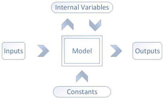

Table 1.
The input details of the model blueprint in Figure 1.
Table 2.
The internal variables, constant parameters, and outputs of the model blueprint in Figure 1.
Figure 2 shows the flow of information from input to output, and the model topology. Here, the individual components can be seen, which will be discussed throughout this section.
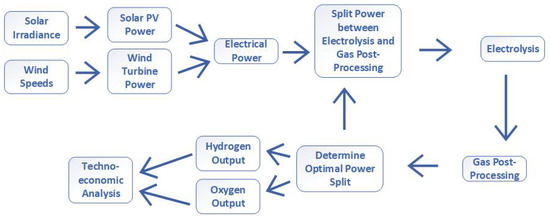
Figure 2.
The energy and information flow of the model, showing the pathway from input electricity to processed gas outputs.
The use of deterministic meteorological data and subsequent power generation sub-models allows for scenario simulations that can be created from arbitrarily-sized generation fleets. Of most interest to the model is the electrolysis potential from wind and solar power in the UK, and these two sources also involve high levels of seasonal, daily, and hourly variation, which leads to complex (and interesting) research conclusions. While more valid, the use of actual generation data from grid statistics is compromised, since in a working grid, operational strategy dictates for curtailments, since priority dispatch is not granted to renewable energy in all cases. Hence, simulation from meteorological data guarantees a maximal ceiling of green electrolysis. There are limitations in the operational range of the stack models, which does result in curtailment; these are recorded in the surplus energy capture statistics. While optimal for renewable energy generators to maximise investment returns by minimising curtailment, 100% surplus capture is not optimal for the whole electrolysis system [4]. This is because a larger electrolysis stack able to capture infrequent maximal peaks for renewable dispatch is either unable to operate in low power input conditions (a minimal power operation threshold) and/or the efficiency (which is dependent on the input power) changes (over the whole range of power inputs), resulting in non-optimal conditions; changing stack power rating for optimal operation is unlikely to be involving the complete capture of renewable energy. For simplicity, the model is configured for direct connection to dedicated renewable generators (wind and solar farms), and renewable energy is purchased at a fixed price per kWh. This removes the complexity of capital, operation, and maintenance costs (amongst others) of the generators from the domain of the model, which, regardless, is outside of the focus. At a national level, there are additional considerations for meteorological variation by location, as well as processing and transmission inefficiencies, which have been excluded as an assumption by considering the national electrical grid as a singular node, and the locations of wind and solar farms as point sources.
3.1. Wind Power
The wind speed data are from NASA’s Power Data [38], set at 50 m, located in Dogger Bank (in the North Sea), the site of multiple current and future GW-scale wind farms. The data set is one year long (2022), with subsequent years of operation assumed to be identical. A well-used approximation for hub height wind speeds [39] compared to the reference (measurement) height above the ground is used, and a ground roughness exponent coefficient is used, set at 0.1 for water. This equation is given as (1),
with the variables as defined: is wind speed at hub height, is the hub height from ground/sea level, is the reference measurement height, and is the ground roughness coefficient. Figure 3 shows the adjusted windspeeds alongside the data from [38] for 2022.
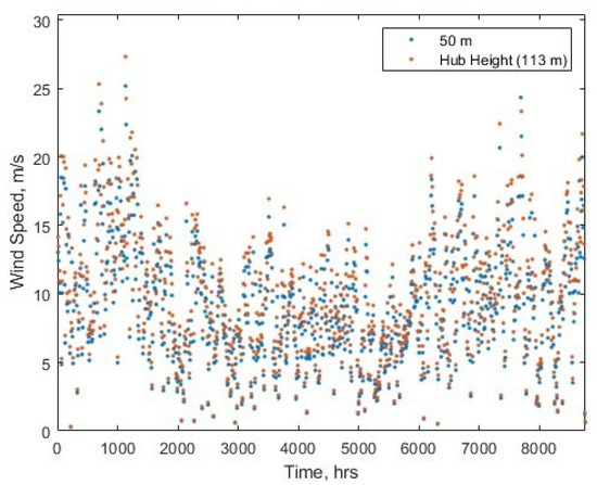
Figure 3.
The windspeeds at Dogger Bank at reference height and calculated for at turbine hub height, for hours in 2022.
The power output for a specific turbine model can be calculated (the Siemens Gamesea Halide-X, rated at 7 MW), using the height-adjusted wind speed. A sample wind power curve is shown in Figure 4, showing the four operational ranges (bins) of wind speeds that result in different performance characteristics [39].
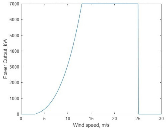
Figure 4.
The characteristic power curve of a Siemens Gamesea Halide-X 7 MW turbine, using [39].
The four bins are separated by three variables defined by the turbine model: cut-in speed (), rated speed (), and cut-off speed (). The first bin is defined from 0 to , where the turbine gives no output below this wind speed. The second bin between and defines power () as (2),
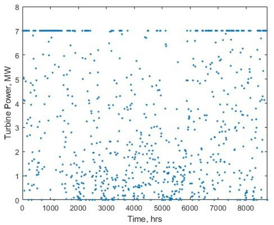
with being the rated maximum power output of the turbine. The third bin is between and , and the power output is the maximum rated turbine power. Above there is no power output, as the turbine is turned off at high wind speeds for safety reasons. The power output is scaled by the number of turbines (a tunable parameter) operating in the system. Figure 5 demonstrates the final wind generation time series for use in the model.
3.2. Solar Power
The solar-PV model utilises a data set generated with a microgrid analytics tool [40], which generated a time series of solar power output hourly for 1 year, at set locations. The data was normalised to apply to a unit square meter, so it can then be rescaled as needed in the model.
There are options to combine the two meteorological data sets into one electrical power time series. Previous work investigated the scenario outcomes from different ratios of renewable generation fleet sizes [41], which is a possible scope for future work.
3.3. Electrolysis Modelling
Water electrolysis at 100% efficiency would result in a mass flow given by (3), with representing the hydrogen mass flow from electrolysis production (kg/s), being the input electrolysis power, and representing the gravimetric energy density of hydrogen (LHV or HHV) in J/kg.
There is naturally inefficiency in the process. Other works have developed characteristic curves that capture the efficiency of electrolyser stacks at different rated power inputs. The core of the electrolysis model can be derived from a power–efficiency relationship. In this work, a 60 kW PEM water electrolyser was chosen [42], as it represents the behaviour of a larger electrolysis stack, which is more appropriate for the operational power ranges of this work. Furthermore, the use of PEM electrolysers over other technologies is seen in many similar studies, likely due to the better case for pairing PEM electrolysis with renewable energy sources. Figure 6 demonstrates the interpolated reproduction that is used to represent the efficiency of water electrolysis. The source material notes a data point on the original plot (71.57 % efficiency at 9.41 kW), which has been included in the figure. This relationship is used to determine the efficiency of water electrolysis for the given input power to the stack.
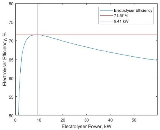
Figure 6.
The replicated curve detailing the relationship between electrolyser power and efficiency, from [42].
Next, an assumption is made that the electrolyser stacks are multiplied by a parameter representing the number of stacks in the ‘fleet’, and that all the stacks receive an identical split of the power and operate identically. A previous work [42] showed the advantages of implementing optimal power-sharing algorithms in a multi-stack system, rather than equal allocation. Optimal power-sharing was not implemented in this work for a number of reasons. Firstly, it would be too crude an assumption that a national-scale fleet of electrolysers would be operating in an optimal condition. Secondly, the implementation of a power-sharing algorithm [42] depended on rates of cell degradation, which is beyond the scope of this research. A minimum power threshold exists; it is set in previous work [42] at 1% of rated power.
Now, the focus can return to the initial electrolytic hydrogen mass flow equation, and include an electrolysis efficiency parameter () (adapted from [43]), as shown in Equation (4).
The label of green hydrogen would only apply if the energy used in electrolysis incurred no carbon emissions. This body of work intends to determine the effects on the inclusion of oxygen in the model. Oxygen, like hydrogen, requires compression or liquefaction for subsequent use down the supply chain. The gas processing energy must also have no carbon footprint, else it would compromise its green status. Thus, the power for gas post-processing must also come from renewable energy power sources. This model assumes that all gas is processed in real time (within the same timestep) alongside electrolytic inception, and fixed gas processing energy requirements per kilogram are used. The assumption used in this model is that the gas processing is carried out in the same timestep as the gases being produced electrolytically, to show the extent of possibility of the process. Further work could be undertaken to include additional processes such as intermediate gas storage between the stacks and the gas compressors.
Therein lies an issue with how to determine the ratio of the power allocation between electrolysis and gas processing. The ratio cannot be determined fundamentally since the electrolyser efficiency () is determined from first principles and then interpolated against input power to determine the mass flow of hydrogen, and since mass flow determines the processing energy requirement, this would create an impossible solving loop to determine the power allocation ratio. Instead, a range of ratios is predetermined, with an increased number of ratio sample points leading to increased accuracy and computational time. For each timestep in the model, the input power is multiplied by an array of values between 0 and 1 for electrolysis power, and the converse 1 to 0 for post-processing power. Within each timestep, each electrolytic power fraction is used to determine the mass flow of hydrogen from the characteristic electrolyser power–efficiency plot. The stoichiometric equivalent yield of oxygen is also calculated for each timestep to determine an oxygen mass flow. The total required gas post-processing (for hydrogen and oxygen) within each timestep at each ratio of power splits can thus be calculated. Next, four ‘checks’ are run, to ensure the validity of the output results, since some input ratios in the range would produce results that are impossible, and need to be filtered from the outputs. These checks are:
- Does the fraction of power devoted to electrolysis not exceed the maximum power of the electrolyser fleet?
- Does the fraction of power devoted to electrolysis exceed the minimum power of the electrolyser fleet?
- Does the fraction of power pre-determined for gas compression equal or exceed the actual amount of gas compression energy required?
- Does the total energy output exceed the energy input?
For each ratio that satisfies all these conditions, the ratio that produces the maximum hydrogen mass flow is selected, along with the corresponding parameters at that point. The mass flow optimisation objective could be changed for another objective in future work, such as a target operating efficiency of the electrolyser.
Summarising this section of the model, the input electricity is split between energy for post-processing (compression or liquefaction) and for electrolysis, resulting in an output of the yield of compressed/liquified gases. Naturally, the electrolysers will not be necessarily running at optimal efficiency conditions since the objective is currently to maximise the processed gas output for the given electricity input. All relevant parameters to observe the operation of the model are recorded, including; required gas post-processing power, electrolyser operating efficiency, gas flow, and surplus energy (power exceeding the electrolyser/post-processing operating range).
3.4. Gas Post-Electrolyser Processing
The energy requirements for hydrogen and oxygen post-processing need to be obtained in order to determine the required energy dedicated for use in each timestep of the model. The specific values are assumed constant; realistically, the energy requirements for compression/liquefaction would be time-dependent as well as sensitive to the type of industrial process used, mass flow, inlet and outlet pressures, and temperatures and system architecture. Simplification to a single constant value (in, for example kWh/kg) for a given process (compression to a set pressure, or liquefaction) is used as an assumption, since subsequent more detailed analysis is outside the scope of the study. Hydrogen is typically compressed to 350 bar for many applications such as transport, and literature also repeatedly mentions of use of liquid hydrogen, to further increase the storage energy density. The processing energy requirements (as constant values) are frequently published, and therefore can be obtained and used directly in this model. For validation, the replicated studies’ own values can be used, and if the value is unavailable, a suitable equivalent value can be used in its place. Oxygen for use elsewhere in industry or other areas is typically produced using pressure swing adsorption or cryogenic air separation. Due to the uniqueness of treating byproduct electrolytic oxygen, similar values for oxygen post-processing energy requirements must be determined. The energy required for the simultaneous liquefaction of hydrogen and oxygen from an electrolyser has been determined as 1.632 kWh/kg [15], and through analysis of the relative mass production rates of the gases in the study and the equivalent energy requirement of hydrogen liquefaction that was included (5.46 kWh/kg), the energy requirement for oxygen liquefaction can be estimated at 1.16 kWh/kg.
A standard storage pressure for compressed oxygen has been nominally selected as 137 bar [44]. The compression energy requirements for oxygen to 137 bar from atmospheric have been determined using Equation (5), with determining the outlet enthalpy of the compressor, for the inlet enthalpy, for the isentropic enthalpy, and for the compressor efficiency. The required energy for gas compression can be found in kWh/kg through derivation from the difference of inlet and outlet enthalpy.
The inlet and isentropic outlet enthalpies were calculated with REFPROP, Version 10.0 [45] for the temperature matching the electrolyser output (80 °C) and chosen electrolyser pressures (atmospheric and 30 bar), and a compression efficiency of 70%. For compression to 137 bar, the compressor required 0.367 kWh/kg from atmospheric pressure, and 0.070 kWh/kg from 30 bar initial pressure. These values, alongside the liquefaction energy requirements are used in the model to provide demonstrative post-processing energy requirements of oxygen.
3.5. Economics Model
The UK Hydrogen Production Costs from 2021 [46] provides a detailed description of the calculation that leads to the levelised cost of hydrogen (LCOH) figure. The net present value (NPV) for total costs calculated each year is divided by the NPV for hydrogen production. The model operates by simulating a year’s input electricity timeseries and subsequent gas production and post-processing, then assuming all subsequent years are identical for economic assessment. The construction costs spread the initial investment CAPEX over the first 3 years, with zero hydrogen output. The CAPEX covers the cost of the electrolyser stacks and the required post-processing costs. Electrolyser stack costs are determined from literature values, typically in or equivalent currency, where specific time-accurate exchange rates can be input by the user. The compressor cost is calculated with a widely used correlation [47] as shown in Equation (6).
The power required for gas compressors (determined separately for hydrogen and oxygen) is the maximum mass flow rate of the gas and the required compression energy per kg. This gives a compressor size (power) and cost necessary in the modelling scenario to process all gas produced in each timestep. This is added to the CAPEX value. It is assumed that for gas liquefaction scenarios, CAPEX costs are same as compressor costs, and scale with the increased power demand and associated increase in cost.
The fixed OPEX is identical for each running year, which considers the operation and maintenance, electricity input costs (assumed identical for each year, except NPV), and water costs, minus the profit from oxygen sales at market rates. The variable OPEX implements a more refined model, which calculates the total operational hours, and when the stack lifetime is in excess of 80,000 h [42], a stack replacement is implemented for that year, at a cost of 60% of the plant CAPEX [46]. This implements the greater resolution of the production time-series of the electrolyser, as opposed to the fixed 11-year limit set initially, since the operational hours will drastically vary between different types of input electricity. The exact parameters in this paragraph are written as sourced from the literature, but can be changed in the model as appropriate. Breaking down the LCOH into subdivisions allows for greater refinement in comparison to other scenario results, since individual contributions to the overall costs can be seen.
4. Results: Model Validation and Demonstration
4.1. Case Study One—Solar Hydrogen in the Atacama Desert
4.1.1. Inputs
Crucial to ensuring the validity in this model and thus its contribution to knowledge is ensuring that the model’s results are consistent with literature and reality. Multi-year, multi-MW projects do not exist yet, which makes the task of validation far more difficult. The more appropriate strategy is to compare it to the outputs of similar models, as best as can be done with given inputs and differing methodologies.
The selected work to make a first comparison simulates Solar-H2 production in the Atacama Desert in Chile, which has some of the highest rates of solar irradiation in the world, and can thus deliver an extremely low cost of solar electricity [30]. It was selected as a comparison piece due to the similarity of modelling topology and aims, but notably differs in key areas that the current work hopes to demonstrate a new contribution. There is a dual advantage in validating the model and displaying outputs as results. The validation will confirm that this model is performing as expected when compared to the reference case, but additionally due to the parallel outputs (with/without oxygen post-processing/sale), direct analysis of the advantages and disadvantages of including oxygen can be seen, and the operational ranges over which any advantages occur.
Some commentary must first be made when showing the reference work [30] as a comparison to this work’s model. The system boundaries are different, since the literature case includes the transportation of hydrogen via ships, with the incurred costs and inefficiencies included. Also, the electrolyser model is much more crude, as it is simply an electricity–hydrogen conversion scalar, of 52–60 kWh/kg for PEM electrolysers, depending on the year when considering efficiency improvements. The LHV for hydrogen energy density was used as well, which is arguably less commonly used in the electrolysis literature, but the new model is able to accommodate either LHV or HHV. Figure 7 shows the required energy per kg for hydrogen, which is in line with the figures given by the reference material [30], of 60 kWh/kg in 2018 and 52 kWh/kg in 2025.
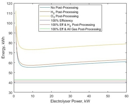
Figure 7.
The required energy per kg for different processes at different electrolyser powers.
USD is used for currency, and the conversion rate was set to USD 1 = GBP 0.80, for any prices that could not be found directly from the source. The following inputs from the reference work [30] have been introduced to the model in order to enact the validation/comparison task:
- Solar input: A solar-PV generation for a standard 1 kW panel array was created using HOMER PRO. This was then scaled to 400 MW to match the literature comparison, as shown in Figure 8;
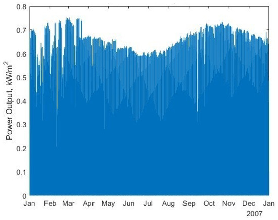 Figure 8. The solar-PV power output per unit area for the selected Atacama Desert location for 2007.
 - Economics Parameters;
- –
- Electrolyser purchase cost, set at $603/kW, which is the median value of the range presented for PEM costs;
- –
- Stack replacement price, at 30% of initial stack price;
- –
- Electricity cost, $0.018/kWh for Solar-PV in 2025;
- –
- Water costs; $3/m3 (equivalent to $0.003/kg);
- –
- Stack lifetime; 65,000 h;
- –
- Operation and maintenance cost; 2% of initial CAPEX per year;
- –
- Project lifetime, 30 years.
The following was also set to make the comparison case, with no mention in the comparison work [30]:
- Market sale price of oxygen $0.14/kg, retrieved as a representative value from a stock market record [48]. It is worth noting that this value could be considered significantly lower than other sources, for example, oxygen is sold at €3.34/kg (approximately $3.76/kg) in another study [17]. On the contrary, oxygen at a range of purities has been recorded at selling between approximately $35–75 a ton in 1994 [13], which adjusting for inflation is between around $0.06 and $0.17/kg;
- Construction time; 3 years [46];
- Discount Rate; 2.5%.
4.1.2. No Gas Post-Processing
The reference work gave an LCOH without post-processing of the hydrogen gas. In the model, by removing the energy requirement for gas post-processing, it is possible to enact a direct comparison of the LCOH between the model and the reference case. The reference case was seeking to meet a hydrogen demand of 16 million kg of H2 per year. In the reference case (PEM electrolyser for 2025), this was achieved with a 345.2 MW installed capacity of electrolysers. To compare to this, the electrolyser count was set to 575,460 kW electrolysers (the equivalent to the source figure of 345.24 MW installed capacity), and the installed solar-PV capacity was varied iteratively. With the set electrolyser fleet size and no compression energy, the 16 million kg annual production is achieved with 1.41 GW of installed solar power, with a resulting LCOH of $1.95/kg, Figure 9. This value is consistent with the PEM photovoltaic direct connection scenarios [30] for 2018 ($3.31/kg) and 2025 ($2.19/kg).
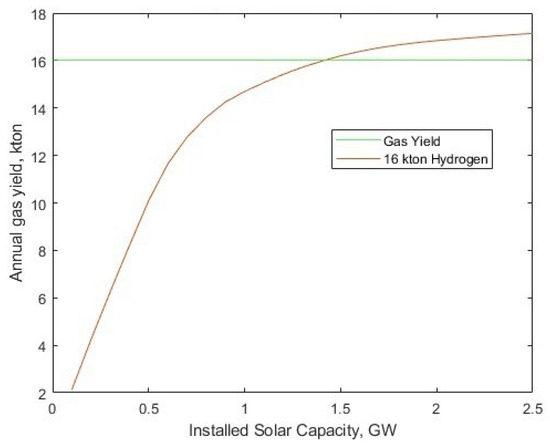
Figure 9.
Hydrogen gas yield per year for different solar-PV fleet sizes, and 345.24 MW electrolyser fleet power, alongside a target 16 kton annual yield.
Worthy of note here is the capacity utilisation factor (CUF) of the solar-PV data set, which gives a 11.73% overall average of rated power, and 35.47% when excluding ‘off’ hours. This low CUF results in the significant capacity difference between rated solar-PV and electrolyser fleet. What should be recognised is the total energy generated by the 1.412 PV array (1.450 TWh, or 5.22 billion MJ), compared to 1.920 billion MJ from 16 kton of hydrogen (120 MJ/kg, LHV) gives an overall electricity to hydrogen conversion efficiency of 36.78% (including wasted PV electricity to surplus). In this scenario, since the solar-PV is bought from the generator at a fixed rate, with no regard to the surplus, the optimal conditions lie in running the electrolysers at the upper end of their power range (i.e., 100%), with no regard for curtailed energy, and this results in 43.49% of the electricity ending as surplus rather than being used for electrolysis, hence the low hydrogen conversion efficiency of 36.78%.
4.1.3. Hydrogen Post-Processing
The reference case gives compression energy requirements from 30 to 200–350 bar of between 1 and 2 kWh/kg. It also states that the energy requirement for compression is not as essential to the overall system due to it being an order of magnitude lower than the electrolysis energy requirement. In this current work’s model, the compression energy is taken from the renewable energy time series, to ensure the compression energy is also zero carbon. The small consideration for hydrogen compression was considered somewhat negligible in the reference work. To compare and validate this, the upper threshold for hydrogen compression energy was used as an input to the model (30 to 350 bar requiring 2 kWh/kg) and the 16 kton per year scenario required 1.448 GW of solar-PV (an increase of 36 MW). Hydrogen compression required 2.15% of the overall energy, although this includes 42.73% of input energy being unused, and remains as surplus energy to the system. Of the used energy, the compression energy made up 3.76% of the total energy used in electrolysis and compression combined. The LCOH rose by USD 0.10/kg to USD 2.05/kg due to hydrogen post-processing energy requirements. With the model now in agreement of outputs with the reference material, the immediate benefits of including oxygen can be observed. The oxygen was liquified with a required energy of 1.16 kWh/kg.
4.1.4. Oxygen Post-Processing
A repeat of the scenario in Figure 9 was performed to determine the new required installed solar capacity to reach 16 kton annual yield, with full oxygen post-processing (liquefaction) included in Figure 10.
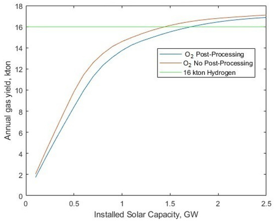
Figure 10.
Hydrogen and oxygen gas yield per year for different solar-PV fleet sizes and 345.24 MW electrolyser fleet power, alongside a target 16 kton annual yield.
Naturally, there is a higher required installed solar capacity of 1.721 GW to account for green energy for additional gas post-processing. However, this reduces the levelised cost to USD 1.33/kg for hydrogen (Figure 11). At the 16 kton per year yield, the O2 post-processing requires USD 0.15/kg of contribution to the CAPEX component of the LCOH, and at all solar capacities, the oxygen saving is USD 1.09/kg.
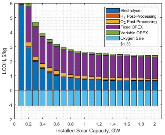
Figure 11.
The LCOH contributions against different solar-PV rated powers. Please note, the hydrogen and oxygen post-processing fractions are CAPEX contributions, the associated power for post-processing is included in the fixed OPEX.
4.1.5. Oxygen Yield Context
Oxygen production yield was compared to the results for sizing electroylsers for hospital oxygen demands, which calculated a 1 MW electrolyser produces 160,570 Nm3 oxygen per year [17], which is 72.8 million kg per year for a 345.24 MW plant. Removing all gas post-processing energy requirements in this model (and noting the change in input solar energy), the annual yield resulted in 131.47 million kg of oxygen per year for a 1.721 GW plant, which is within reasonable margin of the literature result. The discrepancy in results can be explained as follows; the reference material a 1 MW plant is coupled to 1.25 MW of solar-PV (a ratio of 1:1.25), whereas here, a 345.24 MW plant is coupled to 1.721 GW of solar-PV. Setting the scale of the solar-PV array to the same ratio as the reference material (1.25 times larger than the electrolyser fleet, 431.55 MW) yielded 69.903 million kg per year, which is much more in line with the reference yield.
Naturally, there are further operational priorities with co-generation of hydrogen and oxygen to consider in this scenario. Whether the business is interested in reducing the LCOH by any means necessary would mean ensuring a higher installed capacity of solar-PV to contribute to oxygen post-processing. This lowest-LCOH yield-meeting scenario results in a huge amount of surplus energy (Figure 12). The minor differences in electrolysis energy are because the scenario seen here is optimised for the lowest LCOH meeting the 16 kton demand, including oxygen co-production (an installed solar-PV of 1.721 GW), which is not the optimal for the without-oxygen scenario.
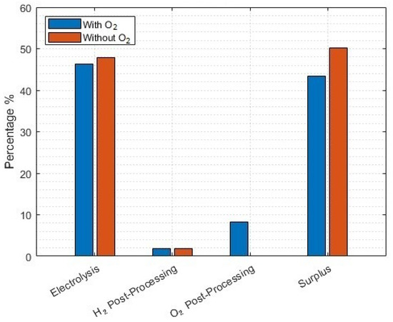
Figure 12.
Energy use of different processes for the lowest-LCOH scenario to meet a 16 kton annual yield. Without oxygen scenarios included where no post-processing energy for oxygen is used, and no profit made on oxygen sales.
4.1.6. Sensitivity of the Number of Electrolysers
The sensitivity of the electrolyser stack fleet size can be determined by setting the solar-PV array to a fixed 1.721 GW. The addition of oxygen post-processing energy requirements is aptly demonstrated to benefit the electrolyser average efficiency beyond 5754 electrolysers (corresponding to the 345.2 MW fleet size as used in the case study comparison [30]) (Figure 13), since the consumption of additional energy for post-processing of oxygen prompts the electrolysers to operate at a higher efficiency point. Despite the additional energy for oxygen post-production, there is only a small compromise in yield as the number of electrolysers is increased, as shown in Figure 14.
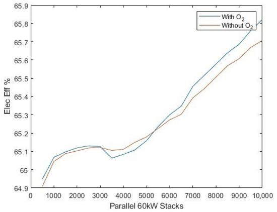
Figure 13.
The average electrolyser efficiency, compared to the number of operation parallel stacks in the system.
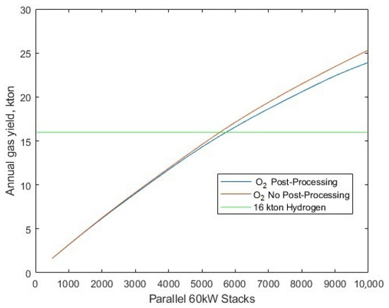
Figure 14.
The annual gas yield compared to the number of operational parallel stacks in the system.
The minimum LCOH, which occurs when using 150,060 kW electrolysers (quantised to nearest the nearest multiple of 250 electrolysers), results in USD 1.40/kg, when using 1.721 GW of solar-PV. The ‘with oxygen’ scenario is clearly advantageous (Figure 15), despite the heavy diverting of would-be electrolysis energy to additional gas post-processes.
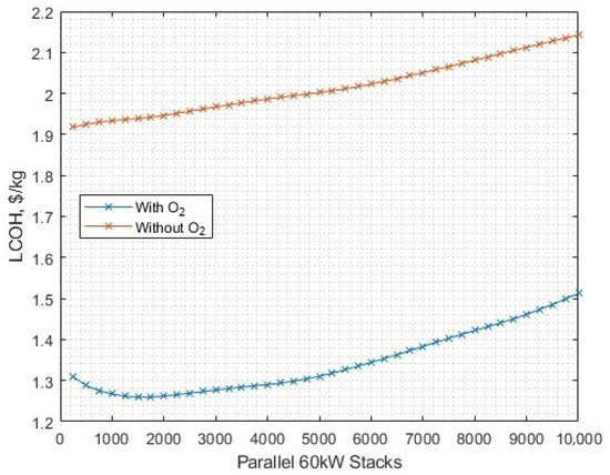
Figure 15.
The sensitivity of the LCOH when compared with the number of operational parallel electrolyser stacks in the system.
4.1.7. No Surplus Electricity Conditions
Removing excessive surplus energy entirely from the scenario would require a significantly larger electrolysis capacity to meet the 16 kton annual demand. In the interest of observing the no-surplus scenarios, the annual demand is ignored, the electrolyser capacity maintained at 345.2 MW and the range of solar-PV capacities significantly reduced. For smaller solar-PV capacities, there is still some surplus energy which is the result of solar-PV electricity generation not meeting the minimum operational threshold of the electrolyser in one timestep (Figure 16). The with-oxygen case has more surplus energy for smaller installed solar-PV capacities as there are more timesteps where too little energy is available to provide for full gas post-processing and electrolysis.
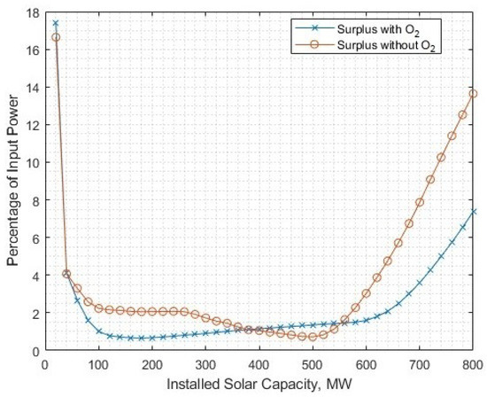
Figure 16.
The remaining surplus energy that is unavoidable in ’no surplus’ scenarios due to the input electricity being below threshold for minimum operational power in the electrolyser. Note that more surplus typically occurs when oxygen is not utillised.
The tradeoff between levelised cost and surplus energy capture is less of an issue when including the utilisation of byproduct oxygen. Figure 17 shows the 5–10% reduction in surplus energy from being absorbed by additional oxygen processing.
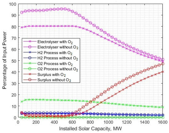
Figure 17.
The benefit of surplus energy reduction, shown by percentage fractions of input power compared at different rated powers of solar-PV generation.
4.1.8. Sensitivity of the Energy for Oxygen Post-Processing
To identify the sensitivity of the oxygen post-processing energy requirement, the solar-PV capacity was set to 1.721 GW and the post-processing energy requirement was varied up to 10 kWh/kg. The crossover of electrolysis energy and oxygen post-processing energy occurs at 6.09 kWh/kg (Figure 18). At this post-processing energy requirement, the LCOH is USD 2.92/kg.
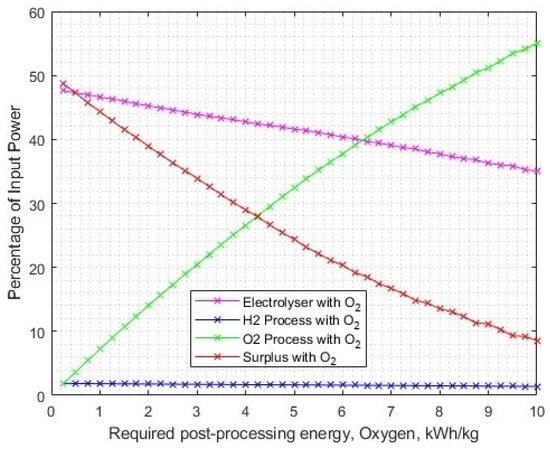
Figure 18.
The change in energy consumptions across different processes, as the required energy for oxygen post-processing increases.
The LCOH crossover occurs at USD 2.02/kg, for 3.28 kWh/kg (Figure 19). This point represents a theoretical upper limit on the oxygen post-processing energy requirements, beyond which it becomes economically unsuitable. However, even the most energetically intensive process (liquifying) is smaller than this value, assuming the limitations (such as constant values for post-processing energy requirements) as used in this model.
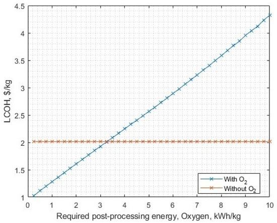
Figure 19.
The sensitivity of LCOH against required oxygen post-processing energy. The no-oxygen utilisation scenario is included as a reference point.
At this crucial crossover point, we can observe how other parameters behave by setting the oxygen post-processing energy requirement to 3.28 kWh/kg and varying the solar-PV size as before. Now the required installed solar-PV capacity is 2.201 GW to meet a 16 kton per year hydrogen yield, with an LCOH of USD 1.93/kg, which is only USD 0.06/kg cheaper than the without oxygen processing/sale alternative, as shown in Figure 20.
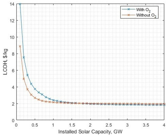
Figure 20.
LCOH against installed solar-PV capacity, with oxygen post-processing energy of 3.28 kWh/kg.
4.1.9. Altering the Amount of Utilised Byproduct Oxygen
The model has a capacity to reduce the amount of byproduct that is utilised, via the ‘oxygen utilisation ratio’, which implies full byproduct processing and sale when equal to 1, and none for 0. Maintaining the 3.28 kWh/kg post-processing energy for oxygen, 1.721 GW of solar-PV capacity (the previous minimum to reach 16 kton at the required energy for liquid oxygen post-processing, 1.16 kWh/kg) and varying the oxygen utilisation ratio, the annual demand can now be met with an oxygen utilisation ratio of 31.52% (Figure 21), but with a slightly more costly LCOH of USD 2.04/kg (Figure 22).
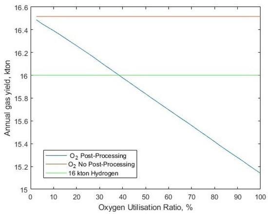
Figure 21.
The hydrogen gas yield compared to oxygen utilisation ratio, with a required oxygen post-processing energy of 3.28 kWh/kg, and no oxygen utilisation/sale is included as a comparison.
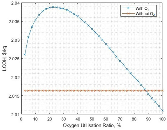
Figure 22.
The LCOH compared to oxygen utilisation ratio, with a required oxygen post-processing energy of 3.28 kWh/kg. No oxygen utilisation/sale is included as a comparison.
These test cases against the reference material scenario clearly show that in nearly all cases, there is an advantage for co-producing oxygen. For a small increase in solar-PV capacity, there is a notable decrease in the LCOH due to cost offsetting from oxygen sale, and the shifting in the power input level to the electrolysers resulting in more efficient production exemplifies this. It has been shown that there is significant sensitivity to the required post-processing energy for oxygen, and if provided with a demand target to reach, this can turn unfavourable.
The chosen post-processing of oxygen (liquefaction) was selected to demonstrate that even an energetically-demanding process is not hugely influential on the outcomes, but delivers a direct financial benefit. The pressurisation of oxygen from atmospheric to 137 bar requires 0.367 kWh/kg, which lowers the solar-PV array size from 1.721 GW to 1.534 GW to meet 16 kton annual demand, and the LCOH falls from USD 1.33/kg to USD 1.09/kg at this point (Figure 23). The reference case implies that the electrolytic gas is at a pressure of 30 bar, which requires only 0.07 kWh/kg for additional pressurisation up to 137 bar. The use of the highest anticipated energy expenditure for oxygen post-processing clearly demonstrates advantages in utilising the byproduct oxygen in nearly every case variation, and thus naturally it can be deduced that lower energy oxygen post-processes would also be beneficial.
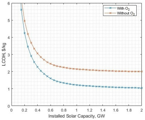
Figure 23.
The LCOH compared to oxygen utilisation ratio, with a required oxygen post-processing energy of 0.367 kWh/kg.
4.2. Case Study Two—UK Offshore Wind
4.2.1. Inputs
The UK government released a white paper in 2021 with scenarios to evaluate the cost of producing hydrogen in line with net-zero strategy [46]. Some of the strategies are in alignment with the architecture of this work’s model and can be used as both a comparison case and validation of the model’s outputs. The high cost 2025 scenario has been chosen to replicate against, since the efficiency of the PEM electrolyser used (1.5 kWh electric input per kWh H2 HHV output, equivalent to 66.67% conversion efficiency) is best matched to the electrolyser in this work’s model. The sample size in the white paper is a 10 MW H2 HHV PEM electrolyser plant (which is equivalent to 13 MW electrical, using the PEM 2025 medium scenario efficiency), and the capacity of the dedicated source is identical (ie 13 MW of dedicated offshore wind). In this validation scenario, since the electrolysers are rated at 60 kW, the plant size was rated as 13.02 MW using 217 stacks. A non-integer number of 7 MW turbines was also used, since 1.86 turbines created a matching power rating. The wind generation load factor falls slightly short of the 51% load factor used in the comparison paper, which is a limitation of the data set used in the model validation. There is an interesting limitation in that surplus power is not included in the scenario, but the further effects of its inclusion can be evaluated in how the LCOH and other parameters also change. Gas post-processing costs costs are not included in the white paper so, as with case 1, the initial validation tests can be performed with gas post-processing energies set to 0 kWh/kg.
Additionally, the following model input data was used:
- Discount/hurdle rate, 10%;
- Stack replacement is listed as every 11 years for PEM. To reflect this, 90,000 h of use time was set as an estimate for 11 years of use. The stack replacement price was 60% of the initial stack CAPEX, as used in the reference;
- Project lifetime, 30 years;
- The CAPEX (the cost of the electrolyser) was converted to GBP/kWe using the low efficiency input, resulting in GBP 973.1283/kWe;
- Fixed OPEX accounts for the operation and maintenance costs. Converting similarly to GBP/kWe is 26.2871, which for a 13 MW plant is GBP 341,732.30 per year. This represents 2.697% of the initial CAPEX, which is the value to be used in the model;
- The electricity cost is GBP 57/MWh;
- Water costs are not mentioned in [46], so they are assumed insignificant in this model. This can be quickly justified using a simple scenario as given from the white paper. A 13 MWe electrolyser at 51% load factor and 77% efficiency [46] produces 871,219 kg hydrogen a year, which would require 9 times the mass of water, i.e., 7,840,971 kg per year, or 7841 tons. The high estimates for water in an arid region such as the Atacama desert were valued at USD 3/m3 [30], equating to approximately GBP 2.40/ton, and so GBP 18,818 per year. The electricity cost for the same plant at GBP 57/MWh would be GBP 3.31m per year, making water costs 0.57% of the electricity cost. This can be considered small enough to ignore for validation purposes. Please note that the water is not included here in Section 4.2 for validation, but is included in Section 4.1 purely on availability of the data;
- Oxygen price remains at USD 0.14/kg (as in case study 1), converted into GBP (GBP 0.11/kg).
4.2.2. No Gas Post-Processing
The LCOH can now be compared between the reference paper [46] and the model, as part of the validation process of this work’s model. The breakdown for the reference case (2025, dedicated offshore wind, high scenario, load factor 51%, PEM) in GBP/kg (Table 3). In addition to this, the initial model run (without oxygen inclusion) is also given alongside.
Table 3.
The comparison between LCOH contributions from [46] and this work’s model.
Worthy of note; in Table 3, the fixed OPEX in the model just represents the O&M and water costs, as opposed to the usual representation of fixed OPEX which includes electricity costs, to allow for the observation of the difference in electricity cost. The differences in LCOH for different breakdowns of the cost can be commented on with regards to load factor and power-dependent efficiency of the electrolysers. The load factor in the white paper is 51%, whereas using the wind data time series in the model, it is only 46.17%. However, the operating efficiencies of the electrolysers (as shown in the histogram in Figure 24) will also contribute to differences elsewhere.
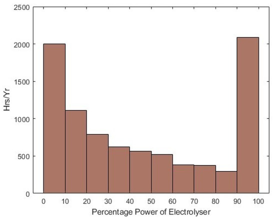
Figure 24.
Histogram showing the distribution of operational power ranges, and the number of hours per year spent in that range.
4.2.3. Hydrogen Post-Processing
The change in LCOH for including hydrogen post-processing is shown, from atmospheric hydrogen, with the hydrogen post-processing energies selected [49] as:
- 350 bar, 2.07 kWh/kg (Theoretical);
- 440 bar for fast refill to 350 bar, 3.22 kWh/kg (Actual measurement);
- 700 bar, 2.37 kWh/kg (Theoretical);
- 700 bar, 3.92 kWh/kg (Actual measurement, including cooling);
- Liquid, 3.36 kWh/kg (Theoretical);
- Liquid, 13.02 kWh/kg (Actual, Existing Medium scale).
Selecting the energy quantity needed for 440 bar (3.22 kWh/kg) increases the LCOH to GBP 6.327/kg, and reduces the lifetime yield from 26.009 to 25.033 million kg. For liquefaction using 13.02 kWh/kg, the LCOH further increases to GBP 7.627/kg and the yield falls to 21.610 million kg over the project lifespan.
4.2.4. Oxygen Post-Processing
The hydrogen post-production was then set at 3.22 kWh/kg (for compression to 350 bar, including 440 bar fast refill), and oxygen post-production (liquefaction, 1.16 kWh/kg) was introduced to investigate how this would affect the levelised cost. By altering the installed wind capacity for a fixed electrolyser fleet size, Figure 25 shows that, at the 13 MW baseline, it is more expensive to include fully utilised byproduct liquid oxygen.
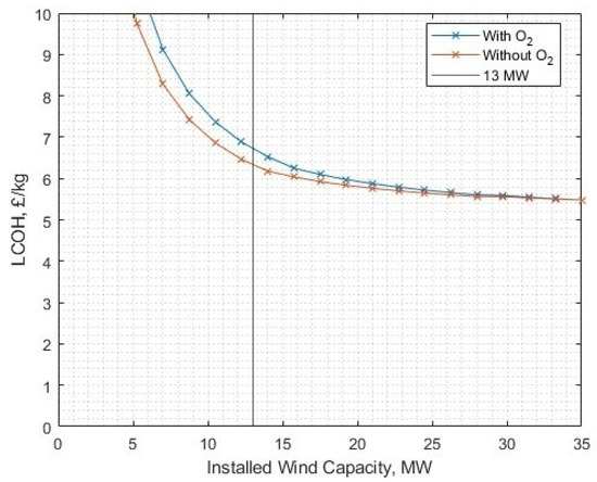
Figure 25.
The levelised cost of hydrogen against the power capacity of the associated wind generation fleet.
4.2.5. Sensitivities of Gas Post-Processing Energies
The sensitivities of different post-production energies for hydrogen are shown in Figure 26 (with no oxygen post-processing), and for oxygen (Figure 27) with 3.22 kWh/kg post-processing of hydrogen, both at the set parameters from the case study. Please note, for the oxygen post-production energy sensitivity analysis, the oxygen is still sold at GBP 0.11/kg regardless of the post-processing energy requirement. The x-axis labels correspond to different energy requirements for different post-production gas delivery formats, as labelled in Table 3 for hydrogen, and in Section 4.1 for oxygen.
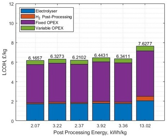
Figure 26.
The LCOH for different post-processing energies of hydrogen, no oxygen included.
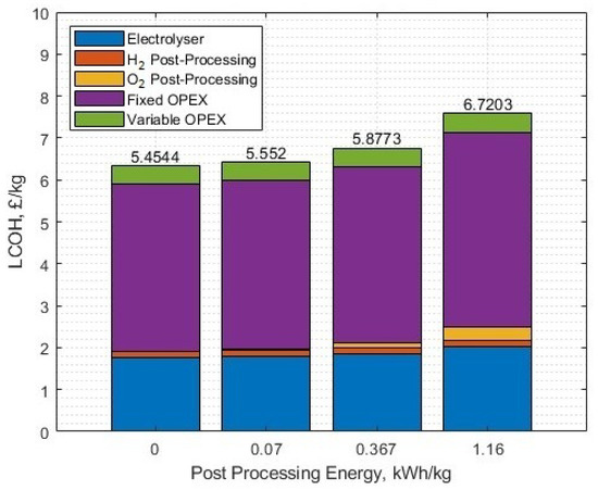
Figure 27.
The LCOH for different post-processing energies of oxygen, with oxygen sale profit subtracted from the fixed OPEX. The post-processing energy of hydrogen is 3.22 kWh/kg.
It is only above 35.123 MW of installed wind capacity (i.e., just over five turbines each rated at 7 MW) that full utilisation of liquid oxygen (with 3.22 kWh/kg hydrogen post-processing energy) becomes beneficial. This represents an electrolyser fleet to wind capacity ratio of 1:2.7. At the 13 MWe plant and wind rated capacity, full oxygen utilisation becomes profitable at a sale price of GBP 0.160/kg, as shown in Figure 28, however, remaining at a price GBP 0.11/kg it is not profitable at any level when altering the ‘oxygen utilisation ratio’, so even only processing a fraction of the byproduct liquid oxygen and selling it at this price is still not favourable.
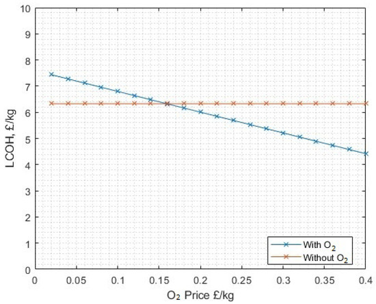
Figure 28.
The sensitivity on LCOH for the sale price of oxygen. The no-oxygen utilisation/sale scenario is included as a comparison.
The changing ratio of utilised oxygen changes the yield of hydrogen (Figure 29), but by considering the change in average electrolyser efficiency (Figure 30), the gradient (of yield to ‘oxygen utilisation ratio’) is reduced compared to a linear trend, since the electrolysers are operating at a better efficiency at higher utilisation ratios, as an increasing proportion of the input power is being diverted to oxygen post-processing, which shifts the mean operational efficiencies higher.
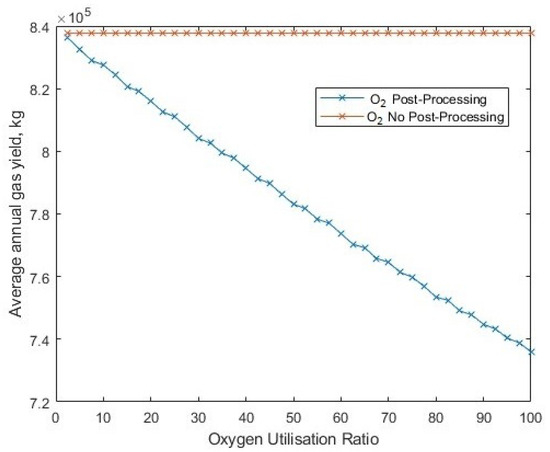
Figure 29.
The change in annual hydrogen yield for different fractions of byproduct oxygen utilisation.
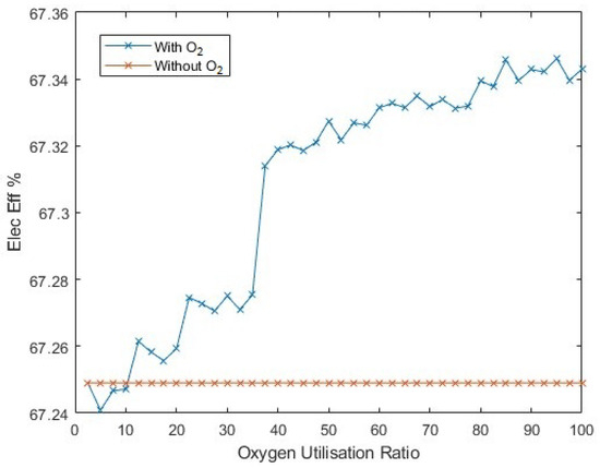
Figure 30.
The change in average electrolyser efficiency for different fractions of byproduct oxygen utilisation.
4.2.6. Mismatched Electrolyser Fleet and Electricity Plant Sizes
What is clear in this exercise is that the assumption used in the white paper [46] of matched electricity plant and electrolyser fleet size does not induce conditions that are favourable for oxygen post-processing to liquid at this price point. Altering the fleet size against the fixed wind generation source (as opposed to the other way around) produces some surplus energy (Figure 31). There is a very narrow margin where (at this price of oxygen) it is beneficial to implement full oxygen post-processing and sale, which is at around 20 to 30 parallel 60 kW stacks, with a LCOH of around GBP 5.15–5.20/kg (Figure 32). At this point, around 75% of the power input becomes surplus. The difference in LCOH occurs due to the reduced availability of power as the number of stacks is increased. For the with-oxygen case, the benefit of sale of by-product oxygen does not outweigh the reduced hydrogen yield as a result of redirecting energy away from electrolysis and into additional oxygen post-processing, for the given conditions in this scenario.
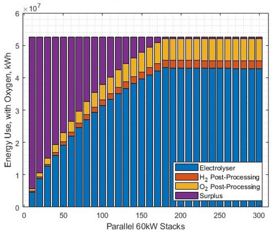
Figure 31.
The energy use for different processes in the system, against the number of parallel operational stacks.
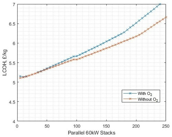
Figure 32.
The LCOH against the number of parallel operational stacks.
4.2.7. Case Study 2 with Solar-PV Input
There is further interest in how solar energy may be considered in a hydrogen (and oxygen) production scenario. Similarly to case study 1, a solar-PV time series was created using HomerPro, with the location set to a generic and representative UK location (Birmingham). In this configuration, solar-PV rated power was increased up to 500 MW (over 13 times the rated power of the electrolysers), and no intersect of with/without oxygen options was found to be preferentially lower LCOH for including oxygen (Figure 33), with oxygen fully utilised in liquid form. At matched solar-PV and electrolyser power capacities (13 MW), the with-oxygen scenario becomes preferential at an oxygen sale price above GBP 0.389/kg, or if the post-processing energy for oxygen is lower than 0.307 kWh/kg, which roughly corresponds to the energy required to compress oxygen to 137 bar. There is no scenario where solely reducing the oxygen utilisation ratio is beneficial.
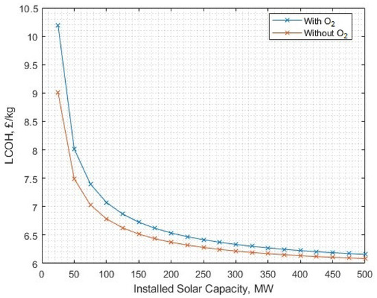
Figure 33.
The LCOH for different levels of associated solar-PV capacity (case study 2).
4.2.8. Oxygen Yield Context
As before in case study 1, the oxygen production yield was compared to an existing study [17], which predicts for a 13 MW electrolyser the oxygen yield will be 2.74 million kg per year. Case study 2 predicts (with 1.25 times more rated wind power than rated electrolyser power, and no gas post-processing energy) an annual yield of 7.74 million kg. The reference number relies on an electrolyser efficiency of 70% [50], compared to the average efficiency in case study 2 of 67.11%, but the load factor of the wind turbine fleet is 46.17%, whereas the load factor of the comparison solar-PV (from [50]) is 14.84%. Repeating the same 13 MW scenario with 1.25 times more solar-PV power (1.25 times 13 MW is 16.25 MW) yields 2.478 million kg per year, which is far closer in yield to the reference case for oxygen generation, mainly since the load factor is 13.18%.
5. Conclusions
The justification for the inclusion of processed byproduct oxygen in electrolytic green hydrogen scenarios has been shown through the creation of a model, and its subsequent use of replicating pre-existing studies for validation, and then in identifying conditions where byproduct oxygen is or is not beneficial. Ultimately, there were limited scenarios in case study 2 (Section 4.2), where fully utilised liquid byproduct oxygen would be beneficial to the LCOH, but there were many in case study 1 (Section 4.1); this in principle shows there is a valid purpose in including oxygen in scenario models of this nature, firstly in an effort to reduce the cost of green hydrogen, and secondly to demonstrate under what conditions (if any) this can be achieved.
The two case studies returned significantly different outcomes for oxygen. This can be explained by the electricity cost, which was a significant fraction of the contribution to total LCOH. The much lower electricity costs used in case study 1 compared to case study 2 provided for many more viable scenarios of beneficial byproduct oxygen inclusion. The context for the electricity costs used in case study 2 are of interest, however, since the predictions for the cost of offshore wind power are still falling, and this will result in benefitting electrolysis scenarios both with and without oxygen co-production. The two case studies returned appropriate yields of oxygen when compared to a similar study [17], when also considering other factors such as power source load factor or electrolyser efficiencies.
The system architecture of the electrolysis fleet being the first customer of a renewable energy generator, and buying in wholesale units of electricity often created optimal scenarios that require large amounts of surplus energy. This is a valid scenario for implementation; however, not every scenario format could permit for this outcome, for example, a smaller electrolyser setup would likely not have primary purchase rights for the renewable energy generator. Furthermore, isolated systems involving generators and electrolysers with no other significant loads would introduce constraints (such as no surplus energy, or generation curtailment). Scenarios that involve using electrolysers to absorb surplus energy after other system loads are met are also of interest within the context of future decarbonised energy systems, and the inclusion of oxygen co-production will be of research interest due to the change in input electricity time series, but also the likely significantly cheaper energy supply.
The implementation of a power–efficiency plot to determine the gas mass production rate for different input electricity magnitudes characterises the role that gas post-processing plays in shifting the efficiency point; for example, reducing the electrolysis input from 60 kW to 50 kW changes the efficiency from 64.7% to 65.7% (Figure 6), which increases the theoretical yield compared to a scalar efficiency coefficient across the same range. The limitations through the assumptions made are important to consider; the electrolysers are all assumed to be identical and receiving the same power input at the same time and thus the estimated power–efficiency readings will be different. The gas post-processing, however, does use scalar coefficients, and subsequent analysis with more complex modelling will be insightful for understanding the associated sensitivities. The limitation of all gas post-processing confined to the same timestep as the gas creation can be further investigated for scenarios where the exclusion of byproduct oxygen is preferred, such as using intermediate gas storage, and post-processing the gas when significant surplus events occur.
Across a select number of parameters, the assessment of oxygen co-production benefits has been shown and to what extent, such as for different oxygen prices, different oxygen utilisation fractions, changes in input renewable power supply, number of parallel electrolyser stacks, and different post-processed gas formats. This ultimately justifies the inclusion of a byproduct oxygen element in green water electrolysis modelling in future energy scenarios. Subsequent models could investigate further changes utilising different electrolyser technologies, more in-depth modelling of the electrochemical and gas handling processes, and different economic environments.
Author Contributions
Conceptualization, C.C.-S.; Data curation, C.C.-S.; Formal analysis, C.C.-S.; Methodology, C.C.-S.; Project administration, V.B. and S.P.; Software, C.C.-S. and J.B.; Supervision, V.B. and S.P.; Validation, C.C.-S.; Writing—original draft, C.C.-S.; Writing—review & editing, Victor Becerra and S.P. All authors have read and agreed to the published version of the manuscript.
Funding
This research was supported by the Faculty of Technology at the University of Portsmouth.
Data Availability Statement
The data presented in this study are available on request from the corresponding author. The data are not publicly available due to the first author’s PhD thesis not having been submitted at the time of publication of this work.
Acknowledgments
The main author (C.C-S.) would like to thank the PhD supervisory team (V.B. and S.P.) for their continuous support and contributions towards this research, and to the Faculty of Technology at the University of Portsmouth for funding via a studentship bursary.
Conflicts of Interest
The authors declare no conflicts of interest.
Abbreviations
The following abbreviations and nomenclature are used in this manuscript:
| LCOH | Levelised Cost of Hydrogen |
| LCOE | Levelised Cost of Electricity |
| PV | Photovoltaic |
| HHV | Higher Heating Value |
| LHV | Lower Heating Value |
| AEL | Alkaline Electrolysis |
| PEM | Proton Exchange Membrane |
| SOEL | Solid Oxide Electrolysis |
| rSOFC | reversible Solid Oxide Fuel Cell |
| CAPEX | Capital Expenditure |
| OPEX | Operational Expenditure |
| CUF | Capacity Utilisation Factor |
| NPV | Net Present Value |
| Wind Speed at Turbine Hub Height, m/s | |
| Turbine Hub Height, m | |
| Reference Wind Speed Measurement Height, m | |
| Ground Roughness Coefficient | |
| Wind Turbine Power Output, W | |
| Wind Turbine Rated Power, W | |
| Turbine Cut-off Speed, m/s | |
| Turbine Rated Speed, m/s | |
| Turbine Cut-in Speed, m/s | |
| Electrolysis Efficiency, % | |
| Hydrogen Mass Flow, kg/s | |
| Electrolyser Power, W | |
| Hydrogen Energy Density, J/kg | |
| Compressor Outlet Enthalpy, kJ/kg | |
| Compressor Isentropic Enthalpy, kJ/kg | |
| Compressor Inlet Enthalpy, kJ/kg | |
| Compressor Efficiency, % |
References
- Fonseca, J.D.; Camargo, M.; Commenge, J.M.; Falk, L.; Gil, I.D. Trends in design of distributed energy systems using hydrogen as energy vector: A systematic literature review. Int. J. Hydrogen Energy 2019, 44, 9486–9504. [Google Scholar] [CrossRef]
- Dozein, M.G.; Jalali, A.; Mancarella, P. Fast frequency response from utility-scale hydrogen electrolyzers. IEEE Trans. Sustain. Energy 2021, 12, 1707–1717. [Google Scholar] [CrossRef]
- Aunedi; Wills, K.; Green, T.; Strbac, G. Net-Zero GB Electricity: Cost-Optimal Generation and Storage Mix. 2021. Available online: https://spiral.imperial.ac.uk/handle/10044/1/88966 (accessed on 23 November 2023).
- González, A.; McKeogh, E.; Gallachóir, B. The role of hydrogen in high wind energy penetration electricity systems: The Irish case. Renew. Energy 2004, 29, 471–489. [Google Scholar] [CrossRef]
- Parra, D.; Valverde, L.; Pino, F.J.; Patel, M.K. A review on the role, cost and value of hydrogen energy systems for deep decarbonisation. Renew. Sustain. Energy Rev. 2019, 101, 279–294. [Google Scholar] [CrossRef]
- Buttler, A.; Spliethoff, H. Current status of water electrolysis for energy storage, grid balancing and sector coupling via power-to-gas and power-to-liquids: A review. Renew. Sustain. Energy Rev. 2018, 82, 2440–2454. [Google Scholar] [CrossRef]
- Williams, J.; Williamson, P.; Parkes, D.; Kirk, K.; Akhurst, M.; Pearce, J. Theoretical Capacity for Underground Hydrogen Storage in UK Salt Caverns; British Geological Survey: Keyworth, UK, 2020.
- Wan, C.; Li, G.; Wang, J.; Xu, L.; Cheng, D.G.; Chen, F.; Asakura, Y.; Kang, Y.; Yamauchi, Y. Modulating Electronic Metal-Support Interactions to Boost Visible-Light-Driven Hydrolysis of Ammonia Borane: Nickel-Platinum Nanoparticles Supported on Phosphorus-Doped Titania. Angew. Chem.-Int. Ed. 2023, 62, e202305371. [Google Scholar] [CrossRef] [PubMed]
- Proost, J. Critical assessment of the production scale required for fossil parity of green electrolytic hydrogen. Int. J. Hydrogen Energy 2020, 45, 17067–17075. [Google Scholar] [CrossRef]
- Sapountzi, F.M.; Gracia, J.M.; Weststrate, C.J.J.; Fredriksson, H.O.; Niemantsverdriet, J.W. Electrocatalysts for the generation of hydrogen, oxygen and synthesis gas. Prog. Energy Combust. Sci. 2017, 58, 1–35. [Google Scholar] [CrossRef]
- Cheng, Y.; Jiang, S.P. Advances in electrocatalysts for oxygen evolution reaction of water electrolysis-from metal oxides to carbon nanotubes. Prog. Nat. Sci. Mater. Int. 2015, 25, 545–553. [Google Scholar] [CrossRef]
- Singla, R.; Chowdhury, K. Enhanced oxygen recovery and energy efficiency in a reconfigured single column air separation unit producing pure and impure oxygen simultaneously. Chem. Eng. Process.-Process Intensif. 2021, 162, 108354. [Google Scholar] [CrossRef]
- Rao, P.; Muller, M. Industrial Oxygen: Its Generation and Use. In ACEEE Summer Study on Energy Efficiency in Industry; American Council for an Energy-Efficient Economy: Washington, DC, USA, 2007. [Google Scholar]
- Kato, T.; Kubota, M.; Kobayashi, N.; Suzuoki, Y. Effective Utilization of By-Product Oxygen from Electrolysis Hydrogen Production; Elsevier Ltd.: Amsterdam, The Netherlands, 2005; Volume 30, pp. 2580–2595. [Google Scholar] [CrossRef]
- Ghorbani, B.; Zendehboudi, S.; Moradi, M. Development of an integrated structure of hydrogen and oxygen liquefaction cycle using wind turbines, Kalina power generation cycle, and electrolyzer. Energy 2021, 221, 119653. [Google Scholar] [CrossRef]
- Paganini, M.; Bosco, G.; Perozzo, F.A.; Kohlscheen, E.; Sonda, R.; Bassetto, F.; Garetto, G.; Camporesi, E.M.; Thom, S.R. The Role of Hyperbaric Oxygen Treatment for COVID-19: A Review; Springer: Berlin/Heidelberg, Germany, 2021; Volume 1289, pp. 27–35. [Google Scholar] [CrossRef]
- Maggio, G.; Squadrito, G.; Nicita, A. Hydrogen and medical oxygen by renewable energy based electrolysis: A green and economically viable route. Appl. Energy 2022, 306, 117993. [Google Scholar] [CrossRef]
- Sridhar, K.R.; Vaniman, B.T. Oxygen production on Mars using solid oxide electrolysis. Solid State Ionics 1997, 93, 321–328. [Google Scholar] [CrossRef]
- National Grid ESO. Future Energy Scenarios 2022. 2022. Available online: https://www.nationalgrideso.com/future-energy/future-energy-scenarios/documents (accessed on 23 November 2023).
- Quarton, C. The Role of Hydrogen Value Chains in Decarbonised Energy Systems. Ph.D. Thesis, University of Bath, Bath, UK, 2021. [Google Scholar]
- Bossel, U.; Eliasson, B. Energy and the Hydrogen Economy. 2003. Available online: https://afdc.energy.gov/files/pdfs/hyd_economy_bossel_eliasson.pdf (accessed on 23 November 2023).
- Andersson, J.; Grönkvist, S. Large-scale storage of hydrogen. Int. J. Hydrogen Energy 2019, 44, 11901–11919. [Google Scholar] [CrossRef]
- Quarton, C.J.; Samsatli, S. Should we inject hydrogen into gas grids? Practicalities and whole-system value chain optimisation. Appl. Energy 2020, 275, 115172. [Google Scholar] [CrossRef]
- Department for Business, Energy & Industrial Strategy. UK Hydrogen Strategy. 2021. Available online: https://www.gov.uk/government/publications/uk-hydrogen-strategy (accessed on 23 November 2023).
- Cioli, M.; Schure, K.M.; Dam, D.V. Decarbonisation Options for the Dutch Industrial Gases Production. 2021. Available online: https://www.pbl.nl/en/publications/decarbonisation-options-for-the-dutch-industrial-gases-production (accessed on 23 November 2023).
- D’Amore-Domenech, R.; Leo, T.J. Sustainable Hydrogen Production from Offshore Marine Renewable Farms: Techno-Energetic Insight on Seawater Electrolysis Technologies. ACS Sustain. Chem. Eng. 2019, 7, 8006–8022. [Google Scholar] [CrossRef]
- Bamisile, O.; Dongsheng, C.; Li, J.; Mukhtar, M.; Wang, X.; Duo, J.; Cao, R.; Huang, Q. An innovative approach for geothermal-wind hybrid comprehensive energy system and hydrogen production modeling/process analysis. Int. J. Hydrogen Energy 2022, 47, 13261–13288. [Google Scholar] [CrossRef]
- Khalid, F.; Bicer, Y. Energy and exergy analyses of a hybrid small modular reactor and wind turbine system for trigeneration. Energy Sci. Eng. 2019, 7, 2336–2350. [Google Scholar] [CrossRef]
- Fragiacomo, P.; Genovese, M. Technical-economic analysis of a hydrogen production facility for power-to-gas and hydrogen mobility under different renewable sources in Southern Italy. Energy Convers. Manag. 2020, 223, 113332. [Google Scholar] [CrossRef]
- Gallardo, F.I.; Ferrario, A.M.; Lamagna, M.; Bocci, E.; Garcia, D.A.; Baeza-Jeria, T.E. A Techno-Economic Analysis of solar hydrogen production by electrolysis in the north of Chile and the case of exportation from Atacama Desert to Japan. Int. J. Hydrogen Energy 2021, 46, 13709–13728. [Google Scholar] [CrossRef]
- Carmo, M.; Fritz, D.L.; Mergel, J.; Stolten, D. A comprehensive review on PEM water electrolysis. Int. J. Hydrogen Energy 2013, 38, 4901–4934. [Google Scholar] [CrossRef]
- Fragiacomo, P.; Genovese, M. Modeling and energy demand analysis of a scalable green hydrogen production system. Int. J. Hydrogen Energy 2019, 44, 30237–30255. [Google Scholar] [CrossRef]
- GigaStack. Available online: https://itm-power.com/projects/gigastack (accessed on 23 November 2023).
- Hodges, A.; Hoang, A.L.; Tsekouras, G.; Wagner, K.; Lee, C.Y.; Swiegers, G.F.; Wallace, G.G. A high-performance capillary-fed electrolysis cell promises more cost-competitive renewable hydrogen. Nat. Commun. 2022, 13, 1304. [Google Scholar] [CrossRef] [PubMed]
- Brauns, J.; Turek, T. Alkaline water electrolysis powered by renewable energy: A review. Processes 2020, 8, 248. [Google Scholar] [CrossRef]
- Olivier, P.; Bourasseau, C.; Bouamama, P.B. Low-temperature electrolysis system modelling: A review. Renew. Sustain. Energy Rev. 2017, 78, 280–300. [Google Scholar] [CrossRef]
- Martinez, D.; Zamora, R. MATLAB simscape model of an alkaline electrolyser and its simulation with a directly coupled PV module. Artic. Int. J. Renew. Energy Res. 2018, 8, 552–560. [Google Scholar]
- NASA. Power Data Access Viewer; NASA: Washington, DC, USA, 2021.
- Tebibel, H. Wind Turbine Power System for Hydrogen Production and Storage: Techno-economic Analysis. In Proceedings of the 2018 International Conference on Wind Energy and Applications in Algeria (ICWEAA), Algiers, Algeria, 6–7 November 2018. [Google Scholar]
- HOMER Pro Microgrid Analytics Tool. Available online: https://www.homerenergy.com/index.html (accessed on 23 November 2023).
- Colbertaldo, P.; Agustin, S.B.; Campanari, S.; Brouwer, J. Impact of hydrogen energy storage on California electric power system: Towards 100% renewable electricity. Int. J. Hydrogen Energy 2019, 44, 9558–9576. [Google Scholar] [CrossRef]
- Lu, X.; Du, B.; Zhou, S.; Zhu, W.; Li, Y.; Yang, Y.; Xie, C.; Zhao, B.; Zhang, L.; Song, J.; et al. Optimization of power allocation for wind-hydrogen system multi-stack PEM water electrolyzer considering degradation conditions. Int. J. Hydrogen Energy 2022, 48, 5850–5872. [Google Scholar] [CrossRef]
- Ursúa, A.; Marroyo, L.; Gubía, E.; Gandía, L.M.; Diéguez, P.M.; Sanchis, P. Influence of the power supply on the energy efficiency of an alkaline water electrolyser. Int. J. Hydrogen Energy 2009, 34, 3221–3233. [Google Scholar] [CrossRef]
- Oxygen Cylinder, Medical Grade, Compressed Gas. Available online: https://www.boconline.co.uk/shop/en/uk/oxygen-cylinder-medical-grade-compressed-gas (accessed on 23 November 2023).
- Lemmon, E.W.; Bell, I.H.; Huber, M.L.; McLinden, M.O. NIST Standard Reference Database 23: Reference Fluid Thermodynamic and Transport Properties-REFPROP, Version 10.0; National Institute of Standards and Technology, Standard Reference Data Program: Gaithersburg, MD, USA, 2018. [CrossRef]
- Department for Business, Energy & Industrial Strategy. Hydrogen Production Costs, 2021. Available online: https://www.gov.uk/government/publications/hydrogen-production-costs-2021 (accessed on 23 November 2023).
- Luyben, W.L. Capital cost of compressors for conceptual design. Chem. Eng. Process.-Process Intensif. 2018, 126, 206–209. [Google Scholar] [CrossRef]
- Intratec. Oxygen Price—Current and Forecast. Available online: https://www.intratec.us/products/water-utility-costs/commodity/oxygen-price (accessed on 23 November 2023).
- Energy Requirements for Hydrogen Gas Compression and Liquefaction as Related to vehicle Storage Needs. 2009. Available online: https://www.hydrogen.energy.gov/docs/hydrogenprogramlibraries/pdfs/9013_energy_requirements_for_hydrogen_gas_compression.pdf?Status=Master (accessed on 23 November 2023).
- Squadrito, G.; Nicita, A.; Maggio, G. A size-dependent financial evaluation of green hydrogen-oxygen co-production. Renew. Energy 2021, 163, 2165–2177. [Google Scholar] [CrossRef]
Disclaimer/Publisher’s Note: The statements, opinions and data contained in all publications are solely those of the individual author(s) and contributor(s) and not of MDPI and/or the editor(s). MDPI and/or the editor(s) disclaim responsibility for any injury to people or property resulting from any ideas, methods, instructions or products referred to in the content. |
© 2024 by the authors. Licensee MDPI, Basel, Switzerland. This article is an open access article distributed under the terms and conditions of the Creative Commons Attribution (CC BY) license (https://creativecommons.org/licenses/by/4.0/).