Article

Novel Custom Loss Functions and Metrics for Reinforced Forecasting of High and Low Day-Ahead Electricity Prices Using Convolutional Neural Network–Long Short-Term Memory (CNN-LSTM) and Ensemble Learning

1
Department of Electrical Engineering and Information Systems, The University of Tokyo, Tokyo 113-8656, Japan
2
Department of Energy Systems Research and Development, KYOCERA Corporation, Yokohama 220-0012, Japan
*
Author to whom correspondence should be addressed.
Energies 2024, 17(19), 4885; https://doi.org/10.3390/en17194885
Submission received: 30 August 2024 / Revised: 23 September 2024 / Accepted: 27 September 2024 / Published: 29 September 2024
(This article belongs to the Section C: Energy Economics and Policy)

Abstract

:
Day-ahead electricity price forecasting (DAEPF) is vital for participants in energy markets, particularly in regions with high integration of renewable energy sources (RESs), where price volatility poses significant challenges. The accurate forecasting of high and low electricity prices is particularly essential, as market participants seek to optimize their strategies by selling electricity when prices are high and purchasing when prices are low to maximize profits and minimize costs. In Japan, the increasing integration of RES has caused day-ahead electricity prices to frequently fall to almost zero JPY/kWh during periods of high RES output, creating significant profitability challenges for electricity retailers. This paper introduces novel custom loss functions and metrics specifically designed to improve the forecasting accuracy of extreme prices (high and low prices) in DAEPF, with a focus on the Japanese wholesale electricity market, addressing the unique challenges posed by the volatility of RES. To implement this, we integrate these custom loss functions into a Convolutional Neural Network–Long Short-Term Memory (CNN-LSTM) model, augmented by an ensemble learning approach and multimodal features. The proposed custom loss functions and metrics were rigorously validated, demonstrating their effectiveness in accurately predicting high and low electricity prices, thereby indicating their practical application in enhancing the economic strategies of market participants.

1. Introduction

1.1. The Importance of High and Low Day-Ahead Electricity Price Forecasting

The 21st century has brought a transformative shift in the global energy sector, driven by the large-scale incorporation of renewable energy sources (RESs) like wind and solar power into electricity grids [1,2]. This transition, motivated by the imperative to mitigate the environmental impacts of traditional energy systems, has introduced substantial fluctuations and uncertainty in electricity generation. The intermittent nature of RES, characterized by fluctuations in power output due to varying weather conditions, leads to sudden changes in electricity supply, which in turn causes volatility in the day-ahead electricity market. These fluctuations make it challenging to predict electricity prices, thereby complicating the pricing mechanisms in the day-ahead electricity market [3,4], in which electricity is traded for delivery the following day.
Given this context, accurate day-ahead electricity price forecasting (DAEPF) becomes crucial [5]. In wholesale electricity markets, price fluctuations significantly affect the financial performance of electric utilities [6]. In Japan, the structure of the Japanese electricity market is primarily based on deregulation, with the Japan Electric Power eXchange (JEPX) serving as the platform for wholesale electricity trading. The market is overseen by the Ministry of Economy, Trade, and Industry (METI), which ensures that competition remains fair and the market functions efficiently. Unlike in some countries where state authorities directly regulate electricity prices, in Japan, prices are largely determined by market dynamics, including supply–demand balance and the impact of RES integration. The increasing presence of RES has added significant volatility to market prices, further complicating DAEPF efforts.
Effective DAEPF supports a range of market participants, including power producers, consumers, and traders, by enabling optimized bidding, strategic planning, and informed decision-making. The increasing integration of RES adds further complexity to price patterns, making accurate forecasting even more vital [7]. For retailers and consumers, precise DAEPF can lead to substantial economic advantages, facilitating optimized procurement strategies and encouraging proactive demand response initiatives [8]. Accurate forecasting is therefore essential for the stability and efficiency of modern power systems, playing a critical role in the transition to a sustainable energy future.
However, forecasting high and low prices is particularly challenging due to the economic strategies employed by market participants. Selling electricity when prices are high and buying when prices are low is fundamental to maximizing profits and minimizing costs. A nuanced understanding of high and low price dynamics can thus provide significant financial benefits and enhance the overall efficiency of electricity markets. This motivates the need for more sophisticated forecasting models that can accurately predict these price extremes.

1.2. DAEPF Models

To address these challenges, various statistical models, including the Autoregressive Moving Average (ARMA) [9,10] and the Autoregressive Integrated Moving Average (ARIMA) [11,12,13], have been frequently utilized in DAEPF research. Although these models offer a solid foundation, their linear structure can limit their ability to accurately capture the complex non-linear patterns introduced by RES integration and demand fluctuations. Consequently, traditional statistical models may struggle to accurately forecast sudden price anomalies in electricity markets.
In response, machine learning models, particularly those incorporating time-dependent features such as the Long Short-Term Memory (LSTM) network, have gained traction in DAEPF [7,14,15]. These models are better equipped to handle the complex, non-linear relationships and price anomalies in electricity markets. For instance, Lago et al. [16] demonstrates the improved accuracy of neural network models over traditional statistical methods in volatile markets. In our previous work [17], we demonstrated that the Convolutional Neural Network-Long Short-Term Memory (CNN-LSTM) model surpasses standalone LSTM models in both accuracy and computation time. In the CNN-LSTM framework, the CNN functions as a feature extraction mechanism, whereas the LSTM is responsible for modeling temporal dependencies. This hybrid approach not only improves predictive accuracy but also significantly reduces training time, making CNN-LSTM a superior choice for DAEPF across various time series forecasting models.

1.3. Custom Loss-Function-Based Forecasting Methods

Despite the advancements in neural network model architectures, traditional loss functions like mean squared error (MSE) and mean absolute error (MAE) have limitations. These functions treat all errors equally, which may not be optimal in contexts where errors at extreme price values (high or low) carry more weight for market participants [18,19].
To address these shortcomings, researchers have developed custom loss functions tailored to the specific needs of forecasting problems. For instance, Usharani et al. [20] proposed an improved loss function within an LSTM framework specifically for predicting location-specific sea surface temperatures. Unlike the traditional MSE, the novel improved loss function incorporates the natural logarithm of the cumulative squared differences between actual and predicted values. This log-scaled error representation not only outperformed standard models but also significantly reduced processing time. In the context of DAEPF, Nowotarski et al. [21] introduced a method for DAEPF by computing prediction intervals using quantile regression and forecast averaging, which provides reliable prediction intervals for volatile electricity prices. Another innovative approach by Nowotarski et al. [22] introduced an asymmetric loss function for DAEPF. This loss function penalizes overestimations and underestimations differently, reflecting the asymmetric cost implications in electricity trading. Overestimating prices might lead to overbidding and financial losses, while underestimating prices could result in missed opportunities for selling electricity at higher prices. Amjady et al. [23] developed a price forecasting model using a weighted mean absolute percentage error loss function. This approach assigns higher weights to larger errors, ensuring that the model focuses more on significant deviations that could have substantial financial impacts. Similarly, Lago et al. [24] proposed a novel loss function combining MSE with a penalty for forecast values outside a certain confidence interval. This hybrid loss function enhances the model’s ability to predict prices accurately, especially during volatile periods influenced by RESs.
These studies emphasize the importance of custom loss functions, each addressing specific characteristics of forecasting challenges, such as volatility, asymmetry, and large errors. Our work builds upon these principles by proposing custom loss functions specifically aimed at reinforcing the accuracy of high and low price predictions, a critical aspect in DAEPF that has not been sufficiently addressed in prior studies.

1.4. Paper Contribution and Organization

The contributions of this paper are summarized as follows. To address the aforementioned challenges, this study proposes novel custom loss functions specifically designed for reinforced forecasting of DAEPF, with a focus on accurately predicting high and low prices. These custom loss functions are integrated within a CNN-LSTM model, enhanced by an ensemble learning approach with multimodal features, to improve the overall accuracy of the forecasting process, particularly in scenarios where extreme price values are critical.
The key findings of this study demonstrate that the proposed custom loss functions significantly outperform the traditional MAE loss function in capturing high and low price extremes, as validated through comprehensive performance metrics on validation and test sets. These findings highlight the practical applicability of the proposed method in improving decision-making processes for electricity market participants. To the best of the authors’ knowledge, these specific custom loss functions have not been previously utilized in existing studies, making this approach a novel contribution to the field of DAEPF.
The rest of this paper is structured as follows. Section 2 details the custom loss functions adopted in this study. Section 3 presents the CNN-LSTM model, the comprehensive structure of the DAEPF method, and the data architecture of the input features. Section 4 presents the performance metrics of the DAEPF results and demonstrates the effectiveness of the proposed custom loss functions. Lastly, Section 5 summarizes the paper and outlines directions for future work.

2. Weighted Mean Absolute Error (WMAE) Loss-Functions-Assisted Different Aspects of DAEPF

The weighted mean absolute error (WMAE) [25] represents an evolution of the conventional MAE loss function, formulated to allocate differential significance to individual data points within regression tasks. While the MAE computes the average squared difference between predicted and actual values, the WMAE introduces a weight for each term, allowing certain errors to have a more significant impact on the overall loss. This modification enables the model to focus more on specific aspects of the data that are deemed important for the forecasting task, such as high or low prices in the context of DAEPF.

2.1. Rationale for Designing Custom WMAE Loss Functions

In DAEPF, certain periods, such as those associated with high or low electricity prices, are more critical for decision-making than others. Accurately predicting these periods can lead to significant financial benefits for market participants. Therefore, it is essential to design a loss function that places greater emphasis on these critical periods during model training.
The custom WMAE loss functions introduced in this study are specifically designed to enhance the model’s ability to forecast high and low prices by assigning greater importance to errors occurring in these periods. The rationale behind the design of the two custom WMAE loss functions is to directly address the challenges of predicting price spikes and drops, which are often difficult to capture with conventional loss functions like the MAE.
Two custom WMAE loss functions were designed as shown in Equations (1) and (2), each addressing different facets of DAEPF. In Equations (1) and (2),  n represents the total number of data points, while i indicates the i-th data point. The weighting vectors, W 1 i and W 2 i , modify the absolute differences between the predicted value y ^ and the actual value y, where y represents the prices normalized to a 0–1 range with respect to the minimum and maximum values in the dataset.

2.2. High-Price WMAE Loss Functions

This loss function is designed to emphasize the accurate prediction of high prices, which are crucial for maximizing profits in electricity trading. The weight assigned to each term, W 1 i = y i p , increases as the price y i rises ( p > 0 ), with p being a hyperparameter that controls the degree of emphasis on higher prices. In this investigation, two candidate values for p were considered: 1 and 2. This design ensures that the loss function penalizes errors more heavily when the actual price is high, thus encouraging the model to focus on accurately predicting these critical periods.
L high price wmae ( y , y ^ ) = 1 n i = 1 n ( | y i y ^ i | W 1 i ) W 1 i = y i p

2.3. Low-Price WMAE Loss Functions

This loss function focuses on improving the accuracy of low-price forecasts, which are equally important for minimizing costs in electricity trading. The weighting vector W 2 i assigns a higher weight when the price y i is below a specified threshold ( l o w _ t h r e s ). In this investigation, two candidate values for l o w _ t h r e s were considered: 0.05 and 0.1, which are compared with the target variable y i after normalization rather than on the original price scale. When y i l o w _ t h r e s , W 2 i is assigned a weight of 10; otherwise, it is assigned a weight of 1. This ensures that the loss function penalizes errors more severely when the actual price is low, thereby prioritizing the accurate prediction of low-price periods. Both candidate values for l o w _ t h r e s were evaluated to assess their impact on model performance.
L low price wmae ( y , y ^ ) = 1 n i = 1 n ( | y i y ^ i | W 2 i ) W 2 i = 10 if y i l o w _ t h r e s 1 otherwise

2.4. Selection of Hyperparameters

Table 1 shows the candidates of the hyperparameters p and l o w _ t h r e s used in the custom WMAE loss functions L high price wmae and L low price wmae . These parameters were carefully selected to explore different levels of emphasis on high and low prices in the custom WMAE loss functions.
As the primary objective in this study is to demonstrate the flexibility of the custom WMAE loss functions in handling various price ranges by adjusting these hyperparameters but not to identify the optimal values for p and l o w _ t h r e s , to limit the introduction of further uncertainty and to maintain the focus of the study, the hyperparameter search was intentionally restricted to two candidate values for both p and l o w _ t h r e s , respectively. The selected values represent a reasonable range that allows for performance optimization, highlighting how the hyperparameters can be tuned to emphasize price ranges critical for electricity market participants.

2.5. Comparison with Conventional MAE Loss Function

For comparative purposes, the conventional MAE loss function L mae was also implemented, as depicted in Equation (3). While the MAE treats all errors equally, the custom WMAE loss functions prioritize specific periods by assigning higher weights where certain predictions (high and low prices) are more critical.
L mae ( y , y ^ ) = 1 n i = 1 n | y i y ^ i |
By designing and implementing the L high price wmae , L low price wmae , and the MAE loss function, this study aims to test the validity of the two custom WMAE loss functions in improving the accuracy of high and low price forecasts in DAEPF, thereby providing more reliable guidance for market participants. While using the L high price wmae and L low price wmae exactly as the corresponding custom metrics, they are denoted as M high price wmae and M low price wmae , respectively.

3. CNN-LSTM Ensemble Learning Framework

3.1. Convolution Neural Network-Long Short-Term Memory Model

A CNN-LSTM model was developed and applied for DAEPF using the Python Tensorflow keras library due to its proven effectiveness in time series forecasting, as demonstrated in our previous study [17]. The architecture of the proposed CNN-LSTM model is shown in Figure 1, and the hyperparameters are selected the same as in our previous work [17].
The architecture of the CNN-LSTM model starts with an input layer that accepts the input data, followed by a 1D Convolution Layer with a Rectified Linear Unit (ReLU) activation function. A Max Pooling Layer is then applied to reduce the spatial dimensionality of the feature maps. Another Convolution Layer is used next for further feature extraction. This is followed by an LSTM Layer, which is responsible for capturing temporal patterns in the data. The output from the LSTM layer is fed into a Fully Connected (FC) layer to generate the model’s final output. The CNN-LSTM model is compiled with the Adam optimizer, set to a learning rate of 0.001, and uses the custom loss function and corresponding metric defined in this study. To avoid overfitting, the batch size was set to 2048, and the number of training epochs was set to 50, in each training session.
For the sake of simplicity, this study does not compare the performance of the CNN-LSTM model with other deep learning models such as MLP, CNN, RNN, or standalone LSTM. The superiority of the CNN-LSTM model over standalone LSTM has been demonstrated in our previous work [17].

3.2. Ensemble Learning Strategy

Traditional ensemble learning method involves aggregating the outputs of several different machine learning models to make a final prediction, which is a commonly used strategy in ensemble learning. For instance, Iyer et al. [26] proposed a CNN and LSTM-based ensemble learning approach for human emotion recognition using electroencephalogram (EEG) recordings by combining the outputs from the CNN and LSTM models together to enhance prediction accuracy.
In contrast, the ensemble learning approach proposed in our previous work [17] and utilized in this study focuses on improving the robustness of a single neural network architecture, rather than combining multiple different models or varying hyperparameters to enhance prediction accuracy. Our approach addresses the inherent uncertainty of the CNN-LSTM model by conducting 30 training iterations for each custom loss function defined in Section 2. Subsequently, we aggregated all individual predictions from these 30 different models, utilizing a basic averaging technique to create the final ensemble prediction. This ensemble learning approach leverages the central limit theorem and is shown in Equation (4) [17], where N represents the total number of predictions and k refers to the index of each individual prediction. We selected N = 30 iterations for ensemble predictions to ensure the stability and reliability of the model output through statistical averaging.
y ^ ensemble = 1 N k = 1 N y ^ k
For a better understanding, the pseudo-code for the ensemble learning process is provided in Algorithm 1.
Algorithm 1 Ensemble learning procedure [17]
1:
Apply natural logarithmic transformation to the day-ahead electricity prices using (9).
2:
Normalize the training and test data separately.
3:
for  i = 1 to N do
4:
   Train the model to generate prediction y ^ i .
5:
end for
6:
Revert the predicted values to their original scale (undo data normalization).
7:
Perform the exponential transformation to convert the predicted values back using (10) (reverse of the natural logarithmic transformation).
8:
Compute the ensemble prediction y ^ ensemble following (4).
9:
Derive the zero price for y ^ ensemble following (5).

3.3. Zero Price Forecasting

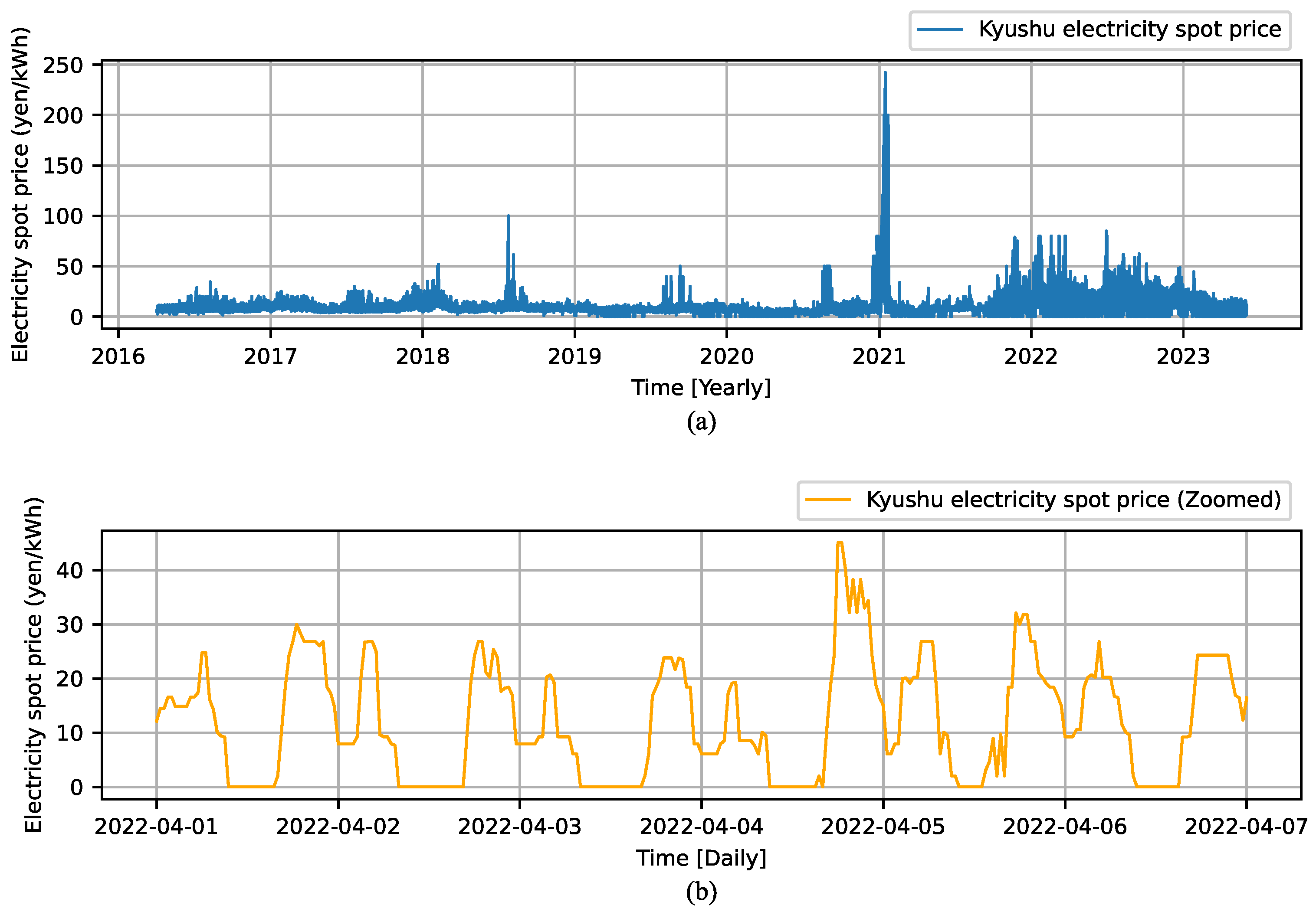
Figure 2a shows the day-ahead electricity prices in the Kyushu area from 5 April 2016 to 31 December 2023, whereas Figure 2b shows an example of a closer view of the zero-inflated prices. As illustrated in Figure 2b, the zero prices in the target variable lead to a zero-inflated regression problem for machine learning models. However, neural networks are generally incapable of consecutively predicting zero values. To address this, in this study, zero prices are forecast by converting any negative model outputs to zeros, as indicated by Equation (5).
y ^ i = max ( 0 , y ^ i )

3.4. Training, Validation, and Test Set

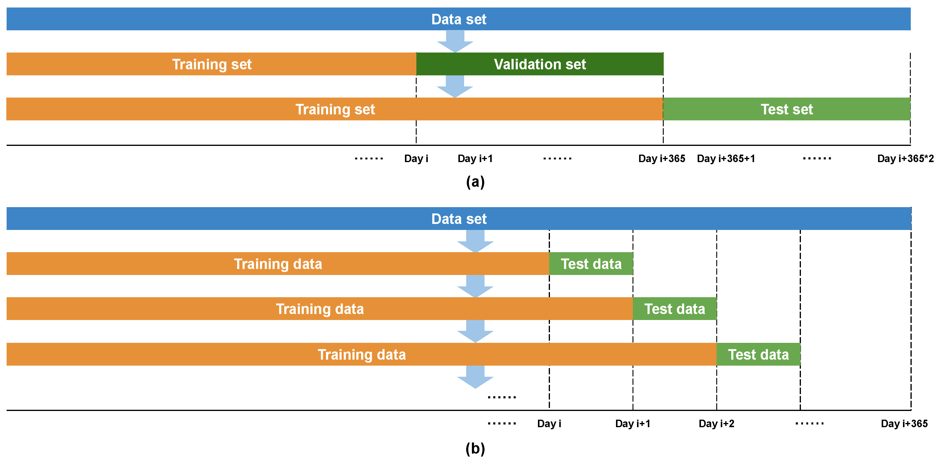
The total dataset was separated into a training set, a validation set, and a test set to select and validate the hyperparameters p and l o w _ t h r e s defined in the custom WMAE loss functions L high price wmae and L low price wmae , as illustrated in Figure 3a. The training data utilized in this study span from 5 April 2016 to the day before the validation set or test set. The validation set and the test set covered the full year of 2022 (1 January 2022–31 December 2022) and the full year of 2023 (1 January 2023–31 December 2023), respectively.

3.5. Performance Evaluation

The performance metrics used for evaluation include the root mean squared error (RMSE), MAE, coefficient of determination ( R 2 ), and the custom WMAE loss functions proposed in this study. The computational formulae for the metrics of RMSE, MAE, and R 2 , are specified in (6)–(8), respectively.
M r m s e ( y , y ^ ) = t = 1 n ( y t y t ^ ) 2 n
M m a e ( y , y ^ ) = 1 n i = 1 n | y i y ^ i |
M R 2 ( y , y ^ ) = 1 t = 1 n ( y t y t ^ ) 2 t = 1 n ( y t y ¯ ) 2

3.6. Data Preparation

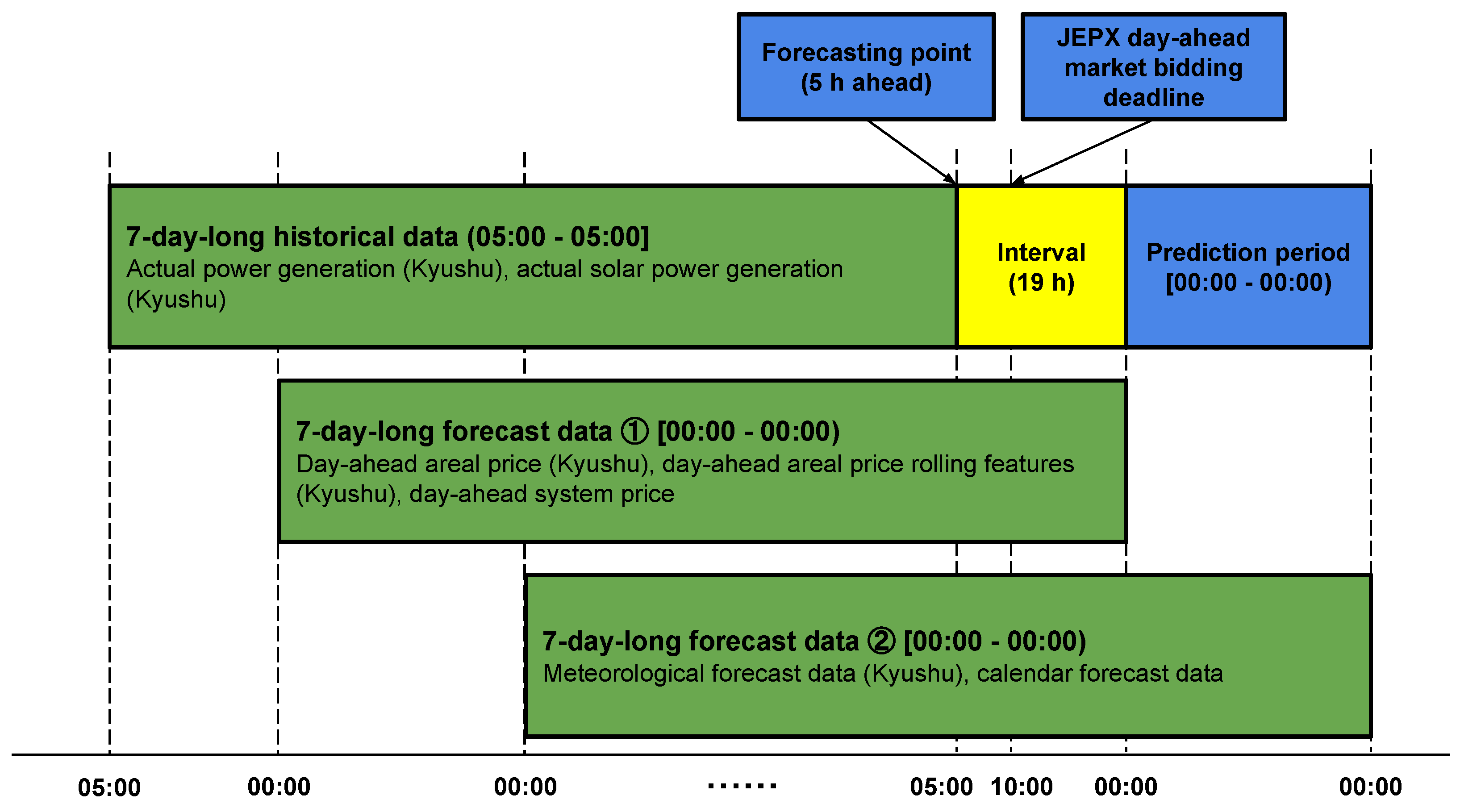
The overall data structure and corresponding time frames are depicted in Figure 4. The input data are divided into three green blocks based on their temporal delays. With a time resolution of 30 min, a 7-day-long moving window was applied to the input data before being input into the CNN-LSTM model. In the JEPX day-ahead electricity market, all bids must be finalized by the 10:00 JST deadline. The forecast was made at 05:00 JST, covering the entire next day from 00:00 JST to 23:30 JST, spanning a total of 48 time slots.
The input data were used as the same in our previous work [17], the validity of which has been verified, comprising the areal day-ahead electricity price (Kyushu); the day-ahead system electricity price [27]; the areal actual power generation (Kyushu) [28]; the areal meteorological forecast data (Kyushu) [29], including the air temperature [30], relative humidity [31], wind speed, cloud cover, accumulated precipitation, and solar radiation; the calendar forecasts, including Japanese national holidays and temporal-cyclic features data; and the rolling features of areal day-ahead electricity prices.

3.7. Logarithmic Transformation Pre-Processing and Exponential Transformation Post-Processing

A natural logarithmic transformation was applied to the target day-ahead electricity prices to reduce skewness and kurtosis in the price data distribution, as defined in Equation (9). After generating the model’s predictions, an exponential reverse transformation was performed to revert the predicted values to their original scale using Equation (10). In Equations (9) and (10), y log and y exp are the logarithmic-transformed target variable and exponentially reversed target variable, respectively.
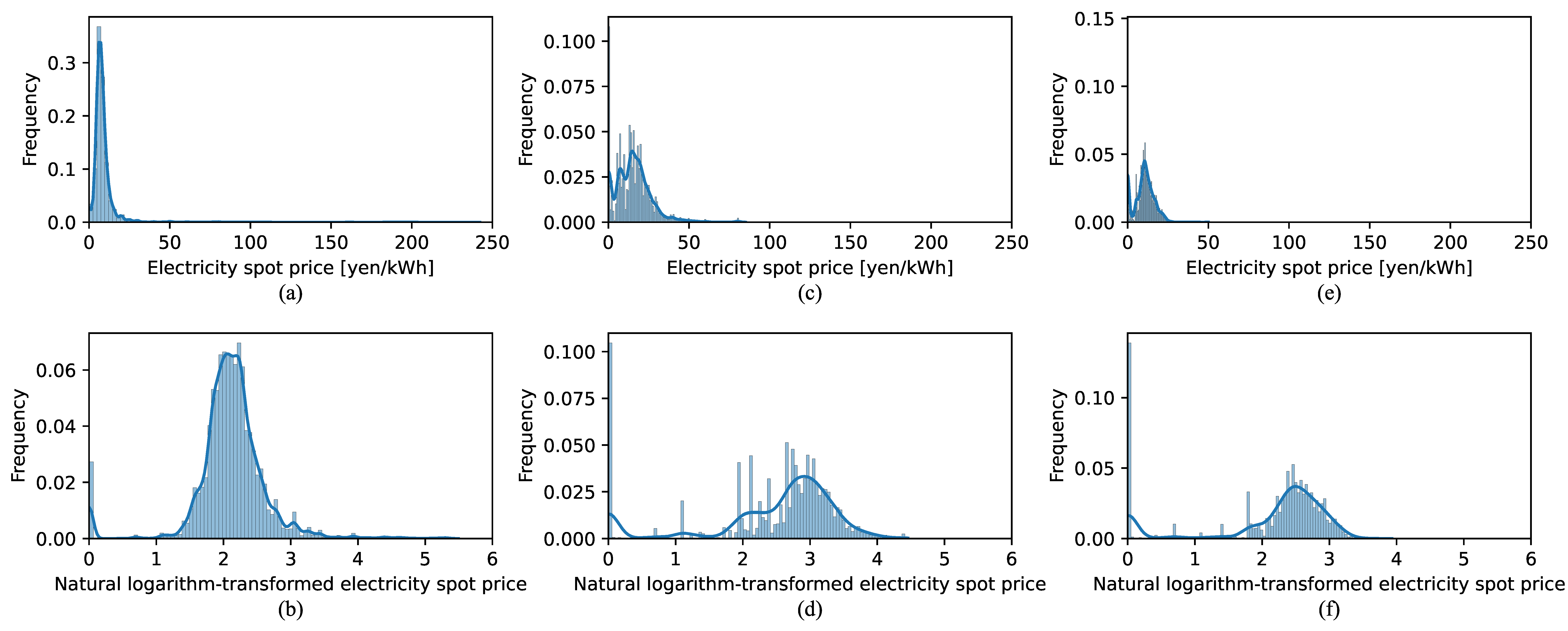
Figure 5 illustrates the distribution of the original day-ahead electricity prices in the Kyushu area and the corresponding natural logarithmic-transformed prices for the training set, validation set, and test set. Table 2 shows the skewness and kurtosis values for both the original and the corresponding natural logarithmic-transformed prices in the three datasets. The training set, which spans a very long range of nearly six years, shows high skewness and kurtosis in the original data, reflecting significant changes in the electricity market and prices over time. After applying the natural logarithmic transformation, there was a significant reduction in both skewness and kurtosis in the training set, indicating that the transformation effectively mitigated the impact of extreme values. In contrast, the validation and test sets, which cover shorter periods and have more stable price distributions, exhibited a shift towards negative skewness after the transformation, with only slight changes in kurtosis. This occurs because the original distributions in the validation and test sets were already relatively symmetric, likely due to their shorter time range of only one year, and the natural logarithmic transformation, by compressing higher values more strongly, introduced negative skewness. Despite the less pronounced effects on the validation and test sets, the transformation is crucial for the training set, as it helps the model achieve higher performance by handling the large price variations and market fluctuations more effectively during training.
y log = log e ( y + 1 )
y exp = e y log 1

3.8. Model Training Platform

The training of the models was conducted using two NVIDIA Quadro RTX 8000 GPUs using the Python keras package in Windows OS.

4. Results and Discussion

Table 3 presents the cross-evaluated performance metrics of the predictions generated by each custom loss function from the CNN-LSTM model, evaluated using each custom metric. This quantitative analysis demonstrates the effectiveness of the custom loss functions proposed in this study, particularly in predicting high and low electricity prices. The key findings from Table 3 are summarized as follows.
  • The L high price wmae effectively reduces its own loss compared to the L mae and the L low price wmae in both validation and test sets, indicating its validity and effectiveness.
  • The L low price wmae effectively reduces its own loss compared to the L mae and the L high price wmae in both validation and test sets, indicating its validity and effectiveness.
  • While either of the L high price wmae or L low price wmae performs best in minimizing its own loss, this comes at the cost of reduced performance in R 2 , MAE, and RMSE metrics.
  • For L high price wmae using p = 2 , the prediction outperforms that obtained with p = 1 for the same metric M high price wmae , whether p = 1 or p = 2 , in both the validation and the test sets. This is achieved with only a slight degradation in R 2 , MAE, and RMSE compared to using p = 1 in L high price wmae , indicating the superiority of p = 2 for L high price wmae .
  • For L low price wmae using l o w _ t h r e s = 0.1 , the prediction outperforms that obtained with l o w _ t h r e s = 0.05 for the same metric M low price wmae , whether l o w _ t h r e s = 0.05 or l o w _ t h r e s = 0.1 , in both validation and test sets. This is achieved with only a slight degradation in R 2 , MAE, and RMSE compared to using l o w _ t h r e s = 0.05 in L low price wmae , indicating the superiority of l o w _ t h r e s = 0.1 for L low price wmae .
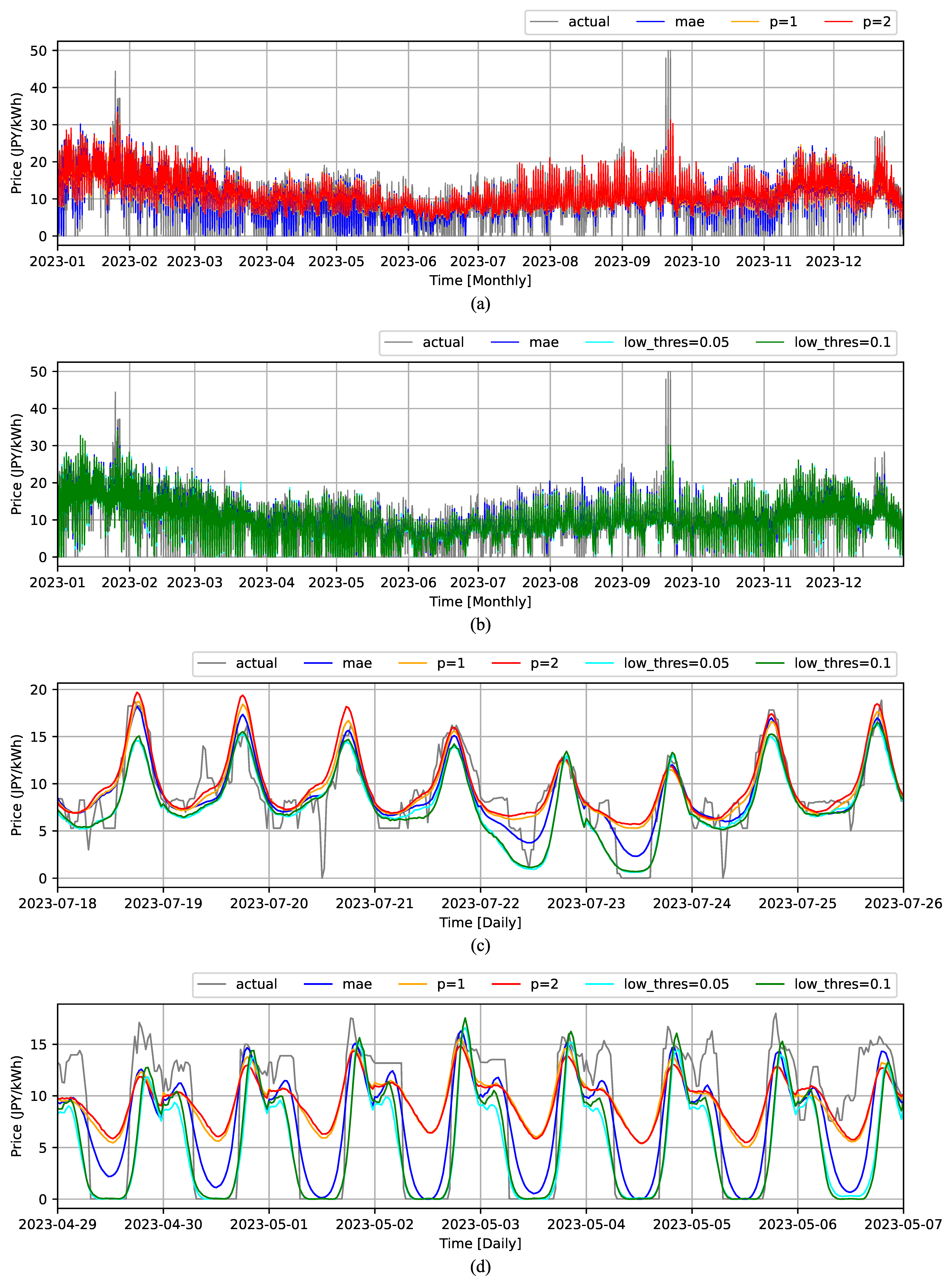
Figure 6 shows the predictions generated by the L high price wmae , L low price wmae , and L mae over the test data. Figure 6a,b show the prediction results over the total one-year-long test range by L high price wmae and L low price wmae , respectively, while Figure 6c,d provide zoomed-in examples demonstrating the superior performance of the L high price wmae and L low price wmae , respectively. Specifically, Figure 6c highlights how L high price wmae excels in predicting high prices, and Figure 6d shows how L low price wmae excels in predicting low prices.
As can be observed from Figure 6a,c, the L high price wmae performs better in capturing high prices compared to the L mae . Similarly, Figure 6b,d demonstrate that the L low price wmae significantly improves the prediction of zero prices compared to the L mae .
In Figure 6c, when p = 2 is used, the L high price wmae generates higher peaks compared to p = 1 , which aligns with the finding from Table 3 that p = 2 is superior to p = 1 for the L high price wmae . Similarly, in Figure 6d, when l o w _ t h r e s = 0.1 is used, the L low price wmae produces lower bottoms compared to l o w _ t h r e s = 0.05 , which aligns with the finding from Table 3 that l o w _ t h r e s = 0.1 is superior to l o w _ t h r e s = 0.05 for the L low price wmae .
The current training and testing strategy involved a single training session followed by testing on a one-year-long range, which inherently introduces variability due to changes over time. Since the primary objective of this study is to evaluate the effectiveness of the proposed custom WMAE loss functions, the day-by-day prediction approach, illustrated in Figure 3b, was not conducted. Our previous study [17] indicates that the day-by-day prediction approach can significantly increase prediction accuracy. However, it is important to note that the primary purpose of Figure 6 is to visually demonstrate the efficacy of the custom WMAE loss functions, rather than to showcase high DAEPF accuracy. Considering the numerous changes that can occur over a year, using the day-by-day prediction approach can achieve much higher accuracy while at the cost of increased computation time.

5. Conclusions and Future Work

5.1. Conclusions

Accurate DAEPF is crucial for effective decision-making among energy market stakeholders, particularly in predicting extreme price fluctuations. This study contributes to the field by introducing two novel custom WMAE loss functions, L high price wmae and L low price wmae , specifically designed for reinforced forecasting of high and low electricity prices, respectively. Unlike previous studies that primarily utilized conventional MAE/MSE loss functions within neural network models, our approach integrates these custom loss functions into a CNN-LSTM framework complemented by multimodal features and an ensemble learning technique. This integration allows the model to place greater emphasis on accurately predicting extreme price values by assigning adaptive weights to prediction errors based on their significance. The effectiveness of the proposed custom WMAE loss functions has been validated as evidenced by the improvements observed in the cross-evaluated performance metrics compared to conventional MAE loss function. For L high price wmae , setting the hyperparameter p = 2 yielded superior performance compared to p = 1 , indicating that a more pronounced focus on high-price errors enhances forecasting accuracy. Similarly, for L low price wmae , a threshold value of l o w _ t h r e s = 0.1 outperformed l o w _ t h r e s = 0.05 , effectively improving low-price predictions by appropriately weighting low-price errors. These findings demonstrate that customizing loss functions to target-specific forecasting challenges can improve model performance in DAEPF. By directly addressing extreme prices, the proposed approach offers more diverse predictions for market participants.

5.2. Future Work

Building upon the promising results of this study, future work will explore novel ensemble learning techniques by integrating predictions from different models that emphasize different aspects of day-ahead electricity prices through different WMAE loss functions, such as the L high price wmae and L low price wmae proposed in this study, to generate improved predictions. Additionally, we aim to further optimize the current custom WMAE loss functions by experimenting with different weighting schemes and hyperparameters to enhance DAEPF performance. Moreover, we plan to investigate the development of custom Weighted Mean Squared Error (WMSE) loss functions to compare their effectiveness against WMAE in capturing extreme price variations. Furthermore, expanding this research to include other machine learning architectures and diverse datasets will also be considered to generalize the applicability and robustness of the proposed approach across various electricity market contexts.

Author Contributions

Conceptualization, Z.W. and R.M.; methodology, Z.W.; software, Z.W.; validation, Z.W. and M.M.; formal analysis, Z.W., T.Y., M.A. and T.N.; investigation, Z.W., M.M., T.Y., M.A., T.N. and R.M.; resources, T.Y, M.A., T.N. and R.M.; data curation, Z.W., T.Y., M.A. and T.N.; writing—original draft preparation, Z.W.; writing—review and editing, Z.W.; visualization, Z.W.; supervision, R.M.; project administration, R.M.; funding acquisition, R.M. All authors have read and agreed to the published version of the manuscript.

Funding

This research was funded by KYOCERA Corporation. This research was conducted by the Social Cooperation Program of Realization of Innovation on Energy and Environment with KYOCERA Corporation in the Graduate School of Engineering at The University of Tokyo.

Institutional Review Board Statement

Not applicable.

Informed Consent Statement

Not applicable.

Data Availability Statement

Not applicable.

Conflicts of Interest

Author Takeshi Yamane, Masato Ajisaka and Tatsuya Nakata were employed by the company KYOCERA Corporation. The remaining authors declare that the research was conducted in the absence of any commercial or financial relationships that could be construed as a potential conflict of interest.

Abbreviations

ARMAAutoregressive Moving Average
ARIMAAutoregressive Integrated Moving Average
CNNConvolutional neural network
CNN-LSTM     Convolutional Neural Network-Long Short-Term Memory
DAEPFDay-ahead electricity price forecasting
EEGElectroencephalogram
FCFully-connected
JEPXJapan Electric Power eXchange
LSTMLong Short-Term Memory
MAEMean absolute error
METIMinistry of Economy, Trade, and Industry
MLPMultilayer Perceptron
MSEMean squared error
R 2 Coefficient of determination
ReLURectified Linear Unit
RESRenewable Energy Source
RMSERoot mean squared error
WMAEWeighted mean absolute error
WMSEWeighted mean squared error
Symbols
eNatural logarithm
ii-th value in a variable sequence
kk-th individual prediction after k-th training of the model
L high price wmae Custom WMAE loss function emphasized on high prices prediction
L low price wmae Custom WMAE loss function emphasized on low prices prediction
L mae Conventional MAE loss function
l o w _ t h r e s Threshold in the L low price wmae
M high price wmae Using L high price wmae as custom metric
M low price wmae Using L low price wmae as custom metric
M m a e Metric of MAE
M R 2 Metric of R 2
M r m s e Metric of RMSE
nSequence length of the target variable
NTotal training times of the model
pPower of the weights in L high price wmae
W 1 i Coefficients of the L high price wmae loss function
W 2 i Coefficients of the L low price wmae loss function
yTarget variable
y ^ Predicted target variable
y ^ ensemble Ensemble prediction of the target variable
y exp Exponentially-reversed target variable
y log Log-transformed target variable

References

  1. Abdelilah, Y.; Bahar, H.; Criswell, T.; Bojek, P.; Briens, F.; Le Feuvre, P. Renewables 2020: Analysis and Forecast to 2025; IEA: Paris, France, 2020. [Google Scholar]
  2. Weitemeyer, S.; Kleinhans, D.; Vogt, T.; Agert, C. Integration of Renewable Energy Sources in future power systems: The role of storage. Renew. Energy 2015, 75, 14–20. [Google Scholar] [CrossRef]
  3. Asiaban, S.; Kayedpour, N.; Samani, A.E.; Bozalakov, D.; De Kooning, J.D.M.; Crevecoeur, G.; Vandevelde, L. Wind and Solar Intermittency and the Associated Integration Challenges: A Comprehensive Review Including the Status in the Belgian Power System. Energies 2021, 14, 2630. [Google Scholar] [CrossRef]
  4. Hua, H.; Qin, Z.; Dong, N.; Qin, Y.; Ye, M.; Wang, Z.; Chen, X.; Cao, J. Data-driven dynamical control for bottom-up energy internet system. IEEE Trans. Sustain. Energy 2022, 13, 315–327. [Google Scholar] [CrossRef]
  5. Özen, K.; Yıldırım, D. Application of bagging in day-ahead electricity price forecasting and factor augmentation. Energy Econ. 2021, 103, 105573. [Google Scholar] [CrossRef]
  6. Wang, K.; Yu, M.; Niu, D.; Liang, Y.; Peng, S.; Xu, X. Short-term electricity price forecasting based on similarity day screening, two-layer decomposition technique and Bi-LSTM neural network. Appl. Soft Comput. 2023, 136, 110018. [Google Scholar] [CrossRef]
  7. Li, W.; Becker, D.M. Day-ahead electricity price prediction applying hybrid models of LSTM-based deep learning methods and feature selection algorithms under consideration of market coupling. Energy 2021, 237, 121543. [Google Scholar] [CrossRef]
  8. Panapakidis, I.P.; Dagoumas, A.S. Day-ahead electricity price forecasting via the application of artificial neural network based models. Appl. Energy 2016, 172, 132–151. [Google Scholar] [CrossRef]
  9. He, K.; Xu, Y.; Zou, Y.; Tang, L. Electricity price forecasts using a Curvelet denoising based approach. Phys. A Stat. Mech. Its Appl. 2015, 425, 1–9. [Google Scholar] [CrossRef]
  10. Yang, Z.; Ce, L.; Lian, L. Electricity price forecasting by a hybrid model, combining wavelet transform, ARMA and kernel-based extreme learning machine methods. Appl. Energy 2017, 190, 291–305. [Google Scholar] [CrossRef]
  11. Chaâbane, N. A hybrid ARFIMA and neural network model for electricity price prediction. Int. J. Electr. Power Energy Syst. 2014, 55, 187–194. [Google Scholar] [CrossRef]
  12. Conejo, A.J.; Plazas, M.A.; Espinola, R.; Molina, A.B. Day-ahead electricity price forecasting using the wavelet transform and ARIMA models. IEEE Trans. Power Syst. 2005, 20, 1035–1042. [Google Scholar] [CrossRef]
  13. Girish, G.P. Spot electricity price forecasting in Indian electricity market using autoregressive-GARCH models. Energy Strategy Rev. 2016, 11–12, 52–57. [Google Scholar] [CrossRef]
  14. Wang, B.; Wang, J. Energy futures price prediction and evaluation model with deep bidirectional gated recurrent unit neural network and RIF-based algorithm. Energy 2021, 216, 119299. [Google Scholar] [CrossRef]
  15. Chen, Y.; Wang, Y.; Ma, J.; Jin, Q. BRIM: An Accurate Electricity Spot Price Prediction Scheme-Based Bidirectional Recurrent Neural Network and Integrated Market. Energies 2019, 12, 2241. [Google Scholar] [CrossRef]
  16. Lago, J.; De Ridder, F.; De Schutter, B. Forecasting spot electricity prices: Deep learning approaches and empirical comparison of traditional algorithms. Appl. Energy 2018, 221, 386–405. [Google Scholar] [CrossRef]
  17. Wang, Z.; Mae, M.; Yamane, T.; Ajisaka, M.; Nakata, T.; Matsuhashi, R. Enhanced Day-Ahead Electricity Price Forecasting Using a Convolutional Neural Network–Long Short-Term Memory Ensemble Learning Approach with Multimodal Data Integration. Energies 2024, 17, 2687. [Google Scholar] [CrossRef]
  18. Hong, W.C. Electric load forecasting by seasonal recurrent SVR (support vector regression) with chaotic artificial bee colony algorithm. Energy 2011, 36, 5568–5578. [Google Scholar] [CrossRef]
  19. Chen, Y.; Li, B. An adaptive functional autoregressive forecast model to predict electricity price curves. J. Bus. Econ. Stat. 2017, 35, 371–388. [Google Scholar] [CrossRef]
  20. Usharani, B. ILF-LSTM: Enhanced loss function in LSTM to predict the sea surface temperature. Soft Comput. 2022, 27, 13129–13141. [Google Scholar] [CrossRef]
  21. Nowotarski, J.; Weron, R. Computing electricity spot price prediction intervals using quantile regression and forecast averaging. Comput. Stat. 2015, 30, 791–803. [Google Scholar] [CrossRef]
  22. Nowotarski, J.; Weron, R. Recent advances in electricity price forecasting: A review of probabilistic forecasting. Renew. Sustain. Energy Rev. 2018, 81, 1548–1568. [Google Scholar] [CrossRef]
  23. Amjady, N. Day-ahead price forecasting of electricity markets by a new fuzzy neural network. IEEE Trans. Power Syst. 2006, 21, 887–896. [Google Scholar] [CrossRef]
  24. Lago, J.; Marcjasz, G.; De Schutter, B.; Weron, R. Forecasting day-ahead electricity prices: A review of state-of-the-art algorithms, best practices and an open-access benchmark. Appl. Energy 2021, 293, 116983. [Google Scholar] [CrossRef]
  25. Zhang, M.; Flores, K.B.; Tran, H.T. Deep learning and regression approaches to forecasting blood glucose levels for type 1 diabetes. Biomed. Signal Process. Control 2021, 69, 102923. [Google Scholar] [CrossRef]
  26. Iyer, A.; Das, S.S.; Teotia, R.; Maheshwari, S.; Sharma, R.R. CNN and LSTM based ensemble learning for human emotion recognition using EEG recordings. Multimed. Tools Appl. 2023, 82, 4883–4896. [Google Scholar] [CrossRef]
  27. Exchange, J.E.P. Day Ahead Market. 2023. Available online: https://www.jepx.jp/en/electricpower/market-data/spot/ (accessed on 19 August 2023).
  28. Organization for Cross-Regional Coordination of Transmission Operators, Japan. Menu. 2023. Available online: https://occtonet3.occto.or.jp/public/dfw/RP11/OCCTO/SD/LOGIN_login (accessed on 1 August 2023).
  29. Japan Meteorological Business Support Center. Numerical Weather Prediction Model GPV-MSM. 2023. Available online: http://www.jmbsc.or.jp/jp/online/file/f-online10200.html (accessed on 15 July 2023).
  30. Wang, Z.; Matsuhashi, R.; Onodera, H. Towards wearable thermal comfort assessment framework by analysis of heart rate variability. Build. Environ. 2022, 223, 109504. [Google Scholar] [CrossRef]
  31. Wang, Z.; Matsuhashi, R.; Onodera, H. Intrusive and non-intrusive early warning systems for thermal discomfort by analysis of body surface temperature. Appl. Energy 2023, 329, 120283. [Google Scholar] [CrossRef]
Figure 1. Schematic of the architecture of the CNN-LSTM model [17].
Energies 17 04885 g001
Figure 2. Kyushu region day-ahead electricity prices [JPY/kWh] (a) and a closer view of zero-inflated prices (b) [17].
Energies 17 04885 g002
Figure 3. One-time prediction schematic (a) and day-by-day prediction schematic (b).
Energies 17 04885 g003
Figure 4. Illustration of the data structure with a 30-min time interval, highlighting the time delays among different data [17].
Energies 17 04885 g004
Figure 5. Distribution of the Kyushu region day-ahead electricity prices and the respective distributions after applying the natural logarithmic transformation for the training set (5 April 2016–31 December 2021) (a,b), validation set (1 January 2022–31 December 2022) (c,d), and test set (1 January 2023–31 December 2023) (e,f).
Energies 17 04885 g005
Figure 6. DAEPF results by (a) L high price wmae , (b) L low price wmae , (c,d) zoomed-in all custom loss functions.
Energies 17 04885 g006
Table 1. Hyperparameters of the defined custom WMAE loss functions.
p12
l o w _ t h r e s 0.050.1
Table 2. Skewness and kurtosis of the original and natural logarithmic-transformed day-ahead electricity prices in the Kyushu area for the training set (5 April 2016–31 December 2021), validation set (1 January 2022–31 December 2022), and test set (1 January 2023–31 December 2023).
OriginalLog-Transformed
Training setSkewness8.77−0.68
Kurtosis123.003.81
Validation setSkewness1.23−1.34
Kurtosis3.981.03
Test setSkewness0.14−1.41
Kurtosis0.520.69
Table 3. Cross-evaluated performance metrics of the proposed custom WMAE loss functions in the validation and test sets.
MetricsValidation Set
L high price wmae L mae L low price wmae
p = 1p = 2 low _ thres  = 0.05 low _ thres  = 0.1
M high price wmae p = 190.70989.73694.445115.319113.252
p = 22866.3852745.9503049.6773689.8233580.916
M R 2 0.5550.5510.5920.4910.489
M m a e 5.5025.5255.1125.5595.515
M r m s e 7.2507.2826.9417.7587.772
M low price wmae l o w _ t h r e s = 0.0514.43514.30110.9199.2678.824
l o w _ t h r e s = 0.114.49514.36610.9639.2908.846
Test set
M high price wmae p = 121.08820.88023.28930.08329.442
p = 2333.394326.820367.711470.263459.550
M R 2 0.5800.5570.6880.6340.642
M m a e 2.8452.8992.4812.6852.633
M r m s e 3.9804.0883.4323.7133.673
M low price wmae l o w _ t h r e s = 0.0512.08812.5207.5735.6005.426
l o w _ t h r e s = 0.112.21012.6487.6745.6745.500
Disclaimer/Publisher’s Note: The statements, opinions and data contained in all publications are solely those of the individual author(s) and contributor(s) and not of MDPI and/or the editor(s). MDPI and/or the editor(s) disclaim responsibility for any injury to people or property resulting from any ideas, methods, instructions or products referred to in the content.