Article

Electric Vehicle Charging Load Prediction Based on Weight Fusion Spatial–Temporal Graph Convolutional Network

by
Jun Zhang
1,
Huiluan Cong
1,
Hui Zhou
1,
Zhiqiang Wang
1,
Ziyi Wen
2,* and
Xian Zhang
2
1
State Grid Shandong Electric Vehicle Service Company Ltd., Jinan 250117, China
2
School of Mechanical Engineering and Automation, Harbin Institute of Technology, Shenzhen 518055, China
*
Author to whom correspondence should be addressed.
Energies 2024, 17(19), 4798; https://doi.org/10.3390/en17194798
Submission received: 30 August 2024 / Revised: 22 September 2024 / Accepted: 24 September 2024 / Published: 25 September 2024

Abstract

:
The rapid increase in electric vehicles (EVs) poses significant impacts on multi-energy system (MES) operation and energy management. Accurately assessing EV charging demand becomes crucial for maintaining MES stability, making it an urgent issue to be studied. Therefore, this paper proposes a novel deep learning-based EV charging load prediction framework to assess the impact of EVs on the MES. First, to model the EV traffic flow, a modified weight fusion spatial–temporal graph convolutional network (WSTGCN) is proposed to capture the inherent spatial–temporal characteristics of traffic flow. Specifically, to enhance the WSTGCN performance, the modified residual modules and weight fusion mechanism are integrated into the WSTGCN. Then, based on the predicted traffic flow, an improved queuing theory model is introduced to predict the charging load. In this improved queuing theory model, special consideration is given to subjective EV user behaviors, such as refusing to join queues and leaving impatiently, making the queuing model more realistic. Additionally, it should be noted that the proposed charging load predicting method relies on traffic flow data rather than historical charging data, which successfully addresses the data insufficiency problem of newly established charging stations, thereby offering significant practical value. Experimental results demonstrate that the proposed WSTGCN model exhibits superior accuracy in predicting traffic flow compared to other benchmark models, and the improved queuing theory model further enhances the accuracy of the results.

1. Introduction

As a promising solution to low-carbon transition, electric vehicle (EV) use is increasing. Their rapid penetration introduces unignorable uncertainties to the electrical loads, posing challenges to the operation of multi-energy systems (MESs). Addressing these challenges is crucial for optimizing MES operation and load management.
The charging load demand can be predicted to effectively quantify the impact of EVs on MESs, providing valuable information for optimizing operations. Most previous studies have used time series analysis methods to predict EV charging loads [1,2,3]. However, time series analysis methods struggle to handle long-term tasks. Recently, researchers have begun to apply deep learning technologies to overcome the limitations of time series analysis methods. Compared to traditional statistical methods, deep learning methods have stronger nonlinear learning capabilities, robustness, and generalization ability, making them particularly suitable for large-scale data processing. For instance, in [4], a long short-term memory (LSTM) model is used to predict EV charging demand at a charging station for the next few hours. In [5], both Sequence to Sequence (Seq2seq) and LSTM are used to predict the EV charging demand, and the study finds that Seq2Seq significantly outperforms other models in multistep prediction. Ref. [6] demonstrates that the LSTM model outperforms the traditional artificial neural network (ANN) in charging load prediction. Ref. [7] compares six different deep neural network models including LSTM, gated recurrent units (GRUs), and their variants and finds that the multivariate LSTM and multivariate GRU are more effective for predicting the EV charging load of fast charging stations (FCSs). Ref. [8] combines ANN and recurrent neural network (RNN), and proposes a novel Q-Learning method for EV load predicting. Ref. [9] proposes an attention-based recurrent convolutional neural network model (LA-RCNN) to predict EV load with consideration of temporal dependencies in multivariate time series. Ref. [10] combines the niche immunity lion algorithm (NILA) and convolutional neural network (CNN) for short-term load prediction of FCSs. Additionally, aware that the charging load of FCSs has both temporal and spatial correlations, some research further studies the spatial–temporal graph convolutional network (STGCN) and its variants. Ref. [11] proposes a heterogeneous STGCN to model the complex spatial–temporal correlations. Based on STGCN, a multistep prediction model is proposed for the load management of charging stations in [12]. Ref. [13] proposes a SEDformer to address the long-term EV load prediction problem. The SEDformer comprises an attention-based temporal encoder and a channel attention-based spatial encoder, which can effectively capture the spatial–temporal characteristics of charging load data.
The above-mentioned charging load predicting methods rely on historical data obtained from FCSs. However, for newly established stations, it is difficult to obtain sufficient and effective historical data. To address the challenges, recent studies explore using traffic flow information to predict the EV charging load instead of using historical data of the FCSs directly. For traffic flow modeling, many researchers utilize deep learning models to capture the complex spatial and temporal characteristics inherent in historical traffic data. For example, in [14], a spatial–temporal fusion graph neural network (STFGNN) is developed for traffic flow forecasting, conducting fusion operations of various spatial and temporal graphs. Ref. [15] proposes a dynamic graph convolutional recurrent network (DGCRN) to model the dynamic characteristics of the correlations among FCSs in the traffic network. Also, ASTNet-T and multi-graph STGCN are introduced to predict charging loads at FCSs directly based on the historical data in [16,17].
Moreover, based on the traffic flow prediction technique, some studies further analyze the charging process in FCS to predict the charging load. For example, in [18], the CNN is used to model traffic flow first and then the queuing theory is applied to predict the EV charging load. Ref. [19] uses wavelet transform and LSTM to predict traffic flow in road networks first, and then uses queuing theory model to convert the predicted traffic flow into EV charging demand. In [20], the traffic flow data from real-time closed-circuit television (CCTV) are used first, and then a Markov chain is applied to determine the charging load. In [21], a speed-flow model is used to simulate the traffic flow of EVs, and the Monte Carlo method is used to simulate EV travel and charging behavior, and finally obtain the charging load. In [22], the traffic flow distribution is modeled by the vehicle mobility model and Dijkstra algorithm first, and then a charging load determination model is proposed, considering multiple charging behaviors. However, most previous studies did not model the spatial–temporal connections inherent in traffic flow when predicting the traffic flow. Moreover, the impacts of subjective EV user behaviors are always ignored in charging load modeling, which leads to predictions that are not accurate enough and lack realism. Therefore, there remains a research gap in developing a high-accuracy charging load prediction method.
From what has been mentioned above, the main challenges that need to be addressed include the following: First, it is difficult to obtain sufficient and effective historical data of newly established FCSs, which makes the traditional historical data-based charging load predicting methods ineffective. Second, in traffic flow modeling, the spatial–temporal connection inherent in traffic data needs to be captured to enhance the predicting accuracy. Third, in charging load prediction, subjective EV user behaviors would significantly influence modeling accuracy, and they need to be explored to facilitate accurate load prediction. Therefore, this paper develops a deep learning-based charging load prediction model that models both spatial–temporal connections and EV user behavior. The main contributions can be concluded as follows:
(1) A traffic flow-based charging load prediction framework is proposed considering the data insufficiency problem frequently happening in newly established FCSs. Different from traditional historical data-based methods, the traffic flow-based method does not rely on the data obtained from the FCSs. Instead, it uses the traffic flow information in the traffic network and uses queuing theory to quantify the load demand. Therefore, this method successfully addresses the data insufficiency problem and produces an effective load prediction method for the newly established FCSs.
(2) A novel weight fusion-based STGCN (WSTGCN) model is proposed to predict the traffic flow. The spatial–temporal attention mechanism is employed in the proposed WSTGCN model to capture the spatial–temporal correlations of the traffic network. Compared with the traditional STGCN, the improved WSTGCN model modifies the residual modules and integrates the weight fusion mechanism to improve the predicting accuracy. By fusing the recent, daily, and weekly characteristics of traffic flow, the traffic flow prediction result is more accurate.
(3) An improved queuing theory is used to model the queuing process of EVs at FCSs, with special consideration given to the subjective behaviors of EV users. Compared with traditional queuing theory, the improved queuing theory models EV user behaviors, including impatience to leave and refusal to join queues, making the queuing model more comprehensive.
The remainder of this paper is organized as follows. Section 2 introduces the WSTGCN model for traffic flow prediction. Section 3 illustrates the improved queueing model-based EV charging demand modeling. Section 4 shows the numerical simulations to demonstrate the effectiveness of our approach. Section 5 concludes this paper.

2. WSTGCN-Based Traffic Flow Prediction

2.1. WSTGCN Framework

For traffic flow prediction, a novel WSTGCN is developed as an improved variant of ASTGCN [23]. Compared with ASTGCN, the WSTGCN modifies the residual modules and integrates the weight fusion mechanism to improve the prediction accuracy. The framework of the WSTGCN is shown in Figure 1. In the WSTGCN, three different periodic components, including recent, daily periodic and weekly periodic components, are used to extract different periodic features of traffic flow data. In each periodic component, multiple spatial–temporal blocks (ST blocks) are stacked to capture the spatial–temporal features of traffic data. Based on the outputs of these periodic components, the final output of the WSTGCN model can be obtained by the weight fusion mechanism.
The final output of the WSTGCN model can be expressed as follows:
Y ^ = f S T r ( X r | ψ r ) , S T d ( X d | ψ d ) , S T w ( X w | ψ w )
where Y ^ is the predictive output of the WSTGCN, and X r , X d , and X w represent the inputs of the recent, daily periodic and weekly periodic components, respectively, as described in Section 2.2; ψr, ψd, and ψw are the parameters of components; STr(∙), STd(∙), and STw(∙) denote the ST blocks, as described in Section 2.3; f(∙) represents weight fusing of the outputs of the three components, as described in Section 2.4.

2.2. Periodic Components of WSTGCN

To illustrate the periodic components, the traffic flow data are introduced first. The traffic network is defined as an undirected graph with N nodes, and each node is equipped with data sampling facilities. In each traffic node, C traffic features are sampled with sampling frequency f times per day, that is, each node generates a feature vector of length C at each sampling time. And the whole traffic network generates N × C × f data per day. We use x t c , n R to denote the value of the c-th feature of node n at sampling time t, x t c R N to denote the c-th signal all over the network at time t, x t n R C to denote the values of all features of node n at sampling time t, and X t R N×C to denote the values of all features of all nodes at sampling time t. Assume that the current time is tp and the size of the predicting window is Tp. Tr, Td and Tw are the lengths of the inputs of the recent, daily periodic, and weekly periodic components, and they are all integer multiples of Tp. The recent, daily periodic, and weekly periodic components are introduced as follows:
(1)
The recent component
Intuitively, the past traffic flows significantly influence the near-future traffic flows. To capture the dependence between near-future data and recent past data, the recent component is utilized, with its input defined as follows:
X r = X t p T r + 1 , X t p T r + 2 , , X t p T r R N × C × T r
where X r denotes the input of the recent component, including historical traffic flow data from time tpTr to tp.
(2)
The daily periodic component
Due to the regular daily routine of people, traffic data may show repeated patterns, such as daily morning peaks. To model the daily periodic patterns, the daily periodic component is used. This component captures the dependence between traffic data from the same time over the past few days and the predicting time, with its input defined as follows:
X d = X t p - T d T p f + 1 , X t p - T d T p f + 2 , , X t p - T d T p f + T p , X t p - T d T p T p f + 1 , , X t p - T d T p T p f + T p , X t p - f + 1 , , , X t p - f + T p R N × C × T d
where X d denotes the input of the daily periodic component, including the historical data from the past few days and the same period as the predicting period.
(3)
The weekly periodic component
Traffic patterns on Mondays usually resemble those of previous Mondays, but always differ significantly from weekends. To capture these weekly periodic features, the weekly periodic component is designed, with its input defined as follows:
X w = X t p - T w T p f 7 + 1 , X t p - T w T p f 7 + 2 , , X t p - T w T p f 7 + T p , X t p - T w T p T p f 7 + 1 , , X t p - T w T p T p f 7 + T p , X t p - f 7 + 1 , , , X t p - f 7 + T p R N × C × T w
where X w is the input of the weekly periodic component, including historical data from the same weekday and period over the past few weeks as the predicting period.

2.3. Spatial–Temporal Block of WSTGCN

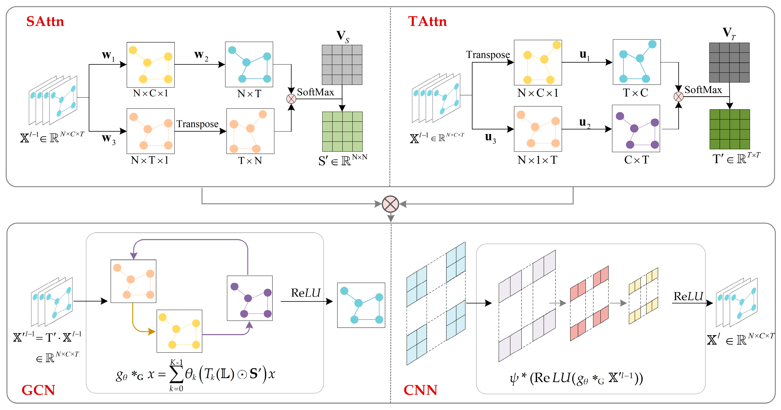
Traffic flow data possess both temporal and spatial attributes. Spatially, traffic conditions at different locations influence each other dynamically. Temporally, correlations exist between traffic conditions across different time slices. To capture the temporal and spatial characteristics simultaneously, spatial–temporal blocks (ST blocks) are employed in the WSTGCN model. In the WSTGCN, each periodic component has stacks of multiple ST blocks. And each ST block is composed of a spatial–temporal attention mechanism (SAttn + TAttn) and a spatial–temporal convolutional network (CNN + GCN). Figure 2 shows an ST block as an example. Assume that this block is the l-th block in the resent component, and the input is X r l 1 = { X 1 , X 2 ,…, X T } ∈ R N×Cl−1×Tl−1.
(1)
Spatial–Temporal Attention Mechanism
The attention mechanism can dynamically adjust weights to prioritize important features, enhancing focus on important time steps or spatial relationships. To adjust the weights of spatial nodes, the spatial attention matrix is used, which can be calculated by the following:
S = V S σ ( ( X r l - 1 w 1 ) w 2 ( w 3 X r l - 1 ) T + b S )
S i , j = exp ( S i , j ) j = 0 N exp ( S i , j )
where S is the spatial attention matrix and S′ is its normalized counterpart to ensure the attention weights of a node sum to 1; Si,j represents the correlation between nodes i and j; w1, w2, w3, VS, and bS are parameters automatically learned by the neural networks; and sigmoid σ is the activation function.
Similarly, the temporal attention matrix adjusts weights to emphasize more significant time steps, which can be calculated by the following:
T = V T σ ( ( X r l - 1 ) T u 1 ) u 2 ( u 3 X r l - 1 ) + b T )
T i , j = exp ( T i , j ) j = 0 T l 1 exp ( T i , j )
where T is the temporal attention matrix and T′ is the normalized counterpart; Ti,j represents the dependent strength between time i and j; and u1, u2, u3, VT, and bT are learnable parameters. Based on the temporal attention matrix, the input can be updated as X r l 1 = { X 1 , X 2 ,…, X′T} = T′∙{ X 1 , X 2 ,…, X T } ∈ R N×Cl−1×Tl−1.
(2)
Spatial–Temporal Convolutional Block
Through the spatial–temporal attention mechanism, the network can automatically pay more attention to valuable spatial and temporal information. Then, the spatial–temporal convolution module is designed to extract the spatial–temporal features of traffic data. The spatial–temporal convolution module consists of a graph convolution and a convolution, as shown in Figure 2.
The graph convolution is used to extract the spatial features of the traffic data. Taking the traffic flow at time t as an example, the c-th feature data point from the traffic network is x = x t c R N. According to [23], the graph convolution operation for x can be expressed as follows:
g θ G x = k = 0 K - 1 θ k T k ( L ) S x
where *G denotes the graph convolution operation; gθ is the convolution kernel; θ R K is the Chebyshev coefficient vector; L = 2L/λmax − In, in which L is the Laplacian matrix of the network graph and λmax is the maximum eigenvalue of the Laplacian matrix; Tk() denotes the Chebyshev polynomial, recursively defined as Tk(x) = 2xTk−1(x) − Tk−2(x), with T0(x) = 0, T1(x) = x. It should be noted that the spatial attention matrix S′ is introduced in Equation (9) to dynamically adjust the weights of the node. Moreover, Equation (9) only illustrates the graph convolution operation for single-channel data x = x t c R N, which can be extended to multiple-channel data. For example, for the recent component, the graph convolution for l-th layer input X r l 1 = { X 1 , X 2 ,…, X′T}∈ R N×Cl−1×Tl−1 can be expressed as gθ *G  X r l 1 .
After the graph convolution operation, the standard 2D convolution operation is used to capture the temporal features of the traffic data. Also, take the operation on the l-th layer in the recent component as an example. The temporal convolution operation is shown as follows:
X r l = Re L U ( ψ * ( Re L U ( g θ G X r l 1 ) ) )
where * denotes a standard convolution operation; ψ are parameters of the temporal dimension convolution kernel; ReLU is the activation function.
(3)
Modified Residual Module
To connect ST blocks, a modified residual module is introduced into the WSTGCN. Compared to the residual module in the ASTGCN, the modified residual module integrates the convolution operation into the residual module, thus making the model training more efficient and stable. The residual module with convolution operations can be expressed as follows:
h ( X l 1 ) = X l 1 + c o n v ( X l 1 )
X l = Re L U ( h ( X l 1 ) + S T ( X l 1 , ψ l ) )
where X l 1 is the input to the l-th ST block; h(∙) is the residual module with a convolution operation; ST(∙) is the operation of the l-th ST block with parameters ψl; X l is the output of the residual module as well as the input of the l + 1-th ST block.

2.4. Weight Fusion Mechanism in WSTGCN

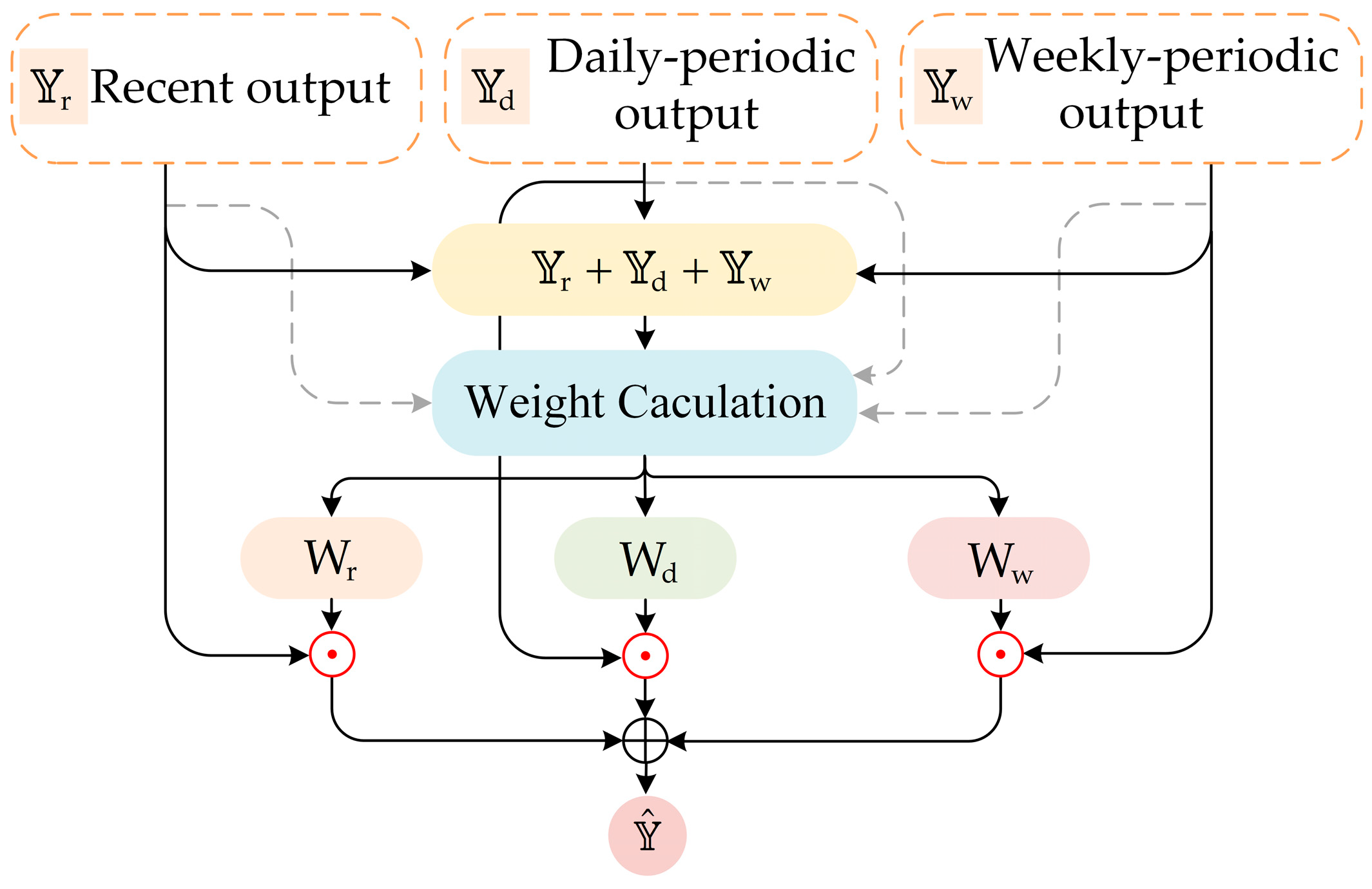
Based on the outputs of periodic components, the weight fusion mechanism is innovatively used to obtain the final output of the WSTGCN. Compared with ASTGCN, which fuses outputs using a fully connected layer, WSTGCN identifies the weight of each component before the fusing operation, resulting in a more reasonable and accurate final output. The weight fusion mechanism is shown in Figure 3.
The weights of recent, daily periodic and weekly periodic components can be calculated by (13)–(15), which reflect the influence and importance of the components on the prediction results.
W r = Y r Y r + Y d + Y w
W d = Y d Y r + Y d + Y w
W w = Y w Y r + Y d + Y w
where Y r , Y d , Y w are the outputs of the present, daily periodic and weekly periodic components, respectively.
Based on the obtained weights, the final prediction result after weight fusion is as follows:
Y ^ = W w Y r + W w Y d + W w Y w
where ⊙ is the Hadamard product.

3. Electric Vehicle Charging Demand Modeling

After obtaining the predicted traffic flow data by WSTGCN, the electrical load of the FCS is analyzed by an improved queueing model. In this improved queueing model, the subjective behaviors of EV users are comprehensively considered, including refusal to join the queue and impatience to leave the queue. By estimating the EV arrival rate and analyzing the queuing process, the FCS charging load can be predicted.

3.1. Electric Vehicle Arrival Rate Estimation

As a key factor for charging load prediction, the arrival rate needs to be estimated first, and it is influenced by the EV state-of-charge (SOC). According to [18], the SOC can be straightforwardly modeled by the consumption power, which can be illustrated by the following:
S O C = 1 p e v D e v E e v
where Eev is the EV battery capacity; pev is the power consumed during the journey; and Dev is the travel distance of the EV. Also, the travel distance under a certain SOC can be obtained by D e v = E e v ( 1 S O C ) / p e v .
However, the travel distance before EVs reach the FCS is difficult to directly determine, especially when the FCS is newly built. To address this challenge, the daily travel distance distribution p(x) and driving in progress distribution g(t) [18], which can be more easily derived from historical data, are used as indirect data sources for estimating travel distance. For example, the daily travel distance probability p(100) = 1% means there is a 1% probability that an EV will travel 100 km in a day. And, a driving in progress probability g(5) = 8% indicates an 8% probability that an EV is on the road at 5 a.m. By using mixture model-based distribution fitting techniques, the probability distribution of daily travel distance and driving in progress can be easily obtained. Based on this distribution, the daily travel distance of an EV arriving at the FCS at time t can be expressed as follows:
D e v , t T = ( E e v ( 1 S O C m ) ) / ( p e v t 0 t g ( t ) d t )
where SOCm represents the mean SOC of EVs when drivers go for charging.
Based on the daily travel distance, the probability that an EV chooses to charge at the FCS at time t can be expressed as follows:
P t = D e v , t T D e v , t 1 T p ( x ) d x
where p(x) is the daily travel distance distribution, which can be obtained by distribution estimation based on the historical data.
Based on the charging probability Pt, the arrival rate is as follows:
λ t = ζ P t f t
where ζ is the penetration rate of EVs, and ft is the predicted traffic flow at time t. It should be noted that since the WSTGCN model is trained on traffic flow data for all vehicle types, including both traditional internal combustion vehicles and EVs, the predicted results from the WSTGCN reflect the total flow of all vehicles. To analyze traffic flow specifically for EVs, the EV penetration rate is utilized. By applying this penetration rate, the traffic flow of EVs can be estimated, allowing for further analysis of the arrival rate at the FCS.

3.2. Improved Queuing Model Considering Driver Behaviors

After arriving at the FCS, EVs queue for charging. To analyze this process, an improved queuing model is proposed in this paper. It assumes that there are C servers in the FCS and up to N cars (N > C) can be in the FCS simultaneously. The number of arriving EVs, denoted as k, follows a Poisson distribution, which can be expressed as follows:
P ( k ) = λ k k ! e λ k = 0 , 1 , 2 , , N
where λ is the average arrival rate.
Also, the charging time of each EV follows an exponential distribution, as shown below:
f ( t c ) = μ e μ t c
where μ is the average leaving rate, which is equal to the number of EVs leaving the FCS. The mean of charging time tc is equal to 1/μ.
It should be noted that some EVs may leave the FCS without charging. To make the analysis more realistic and practical, the refusal to join and impatience to leave behaviors of users are fully considered in the improved queuing model proposed in [18].
Refusal to join behavior occurs when an EV enters an FCS and finds there is a long queue, causing the user to hesitate about joining. This hesitation is influenced by the queue length. The probability of EV choosing to queue is defined as follows:
α k = 1             k < C e ( k C ) σ             C k < N   , σ 0 0             k = N
where σ is the refusal rate parameter. As k increases, the probability of EV users’ willingness to join the queue will decrease.
Moreover, impatience to leave behavior refers to EVs leaving the FCS due to long wait times in the queue. This impatience is primarily related to the number of EVs already in the queue. When there are k EVs in the queue, the number of EV users leaving impatiently can be defined as follows:
β k = 0 k C δ ln ( k C + 1 ) C < k N ,   δ 0
where δ is the leaving rate parameter. As k increases, the number of EVs leaving will also increase.
Considering the two leaving conditions above, the average arriving rate and average leaving rate can be updated as follows:
λ k = λ α k = λ             k < C λ e ( k C ) σ             C k N   , σ 0 0             k = N
μ k = μ β k = μ k C μ δ ln ( k C + 1 ) C < k N
By considering refusal behavior and impatience behavior, the arrival process and charging duration time of EVs can be modeled more precisely, which leaves a solid foundation for the subsequent modeling of the charging load.

3.3. Markov Chain-Based Charging Process Analysis

Based on the arriving rate and leaving rate, the Markov chain is used to model the charging state transitions of EVs, which have two states: arriving and leaving. The state transition diagram is shown in Figure 4.
According to [18], the FCS balance equation can be derived as follows:
( λ k + μ k ) P k = λ k 1 P k 1 + μ k + 1 P k + 1
where Pk is the steady-state probability of the Markov chain at the state k.
By solving (25)–(27), the probability of k EVs simultaneously being in the charging station can be obtained:
P k = λ k μ k k ! P 0 0 k < C λ k e σ ( k C ) ( k C 1 ) / 2 μ k C ! j = 1 k C ( C + δ μ ln ( j + 1 ) ) P 0 C k N
The probability that no EV is in the charging station P0 is given by the following:
P 0 = k = 0 C ρ k k ! + k = C + 1 N λ k e σ ( k C ) ( k C 1 ) / 2 μ k C ! j = 1 k C ( C + δ μ ln ( j + 1 ) ) 1
The number of charging EVs in the FCS can be expressed as follows:
N ch = k = 0 C k λ k μ k k ! P 0 + C k = C + 1 N λ k e σ ( k C ) ( k C 1 ) / 2 μ k C ! j = 1 k C ( C + δ μ ln ( j + 1 ) ) P 0
Furthermore, the charging load of the FCS can be calculated by the following:
P FCS = N ch p ch
where PFCS is the charging load of the FCS, and pch is the charging power of the charger.

4. Experiments

4.1. Performance Evaluation for the WSTGCN Model

4.1.1. Prediction Accuracy Comparison

To validate the proposed WSTGCN, comparative experiments are conducted with 6 benchmark models. The benchmark models are briefly described as follows:
(1) Historical average model (HA): This uses the average value of the past 12 time slices to predict the next value.
(2) Autoregressive integrated moving average model (ARIMA) [24]: ARIMA transforms non-stationary series into stationary time series through multiple differencing first, and then uses stationary time series for predictions.
(3) Long short-term memory network (LSTM) [25]: Thanks to its special gate structure, LSTM can effectively capture useful information in both the long term and short term, thus having excellent predictive ability in time series prediction.
(4) Gated recurrent unit (GRU) [26]: GRU is very similar to LSTM, using a gate mechanism to capture useful information. But GRU only has two gates (i.e., update and reset), compared with LSTM, which has three gates (forget, input, output). Thus, GRU has fewer parameters than LSTM, making it converge faster in training.
(5) Spatial–temporal graph convolutional network (STGCN) [27]: STGCN is composed of multiple spatial–temporal convolution blocks to extract useful spatial and temporal features. Thus, it can efficiently predict time series with a graph structure, like traffic flow data.
(6) Attention-based STGCN (ASTGCN) [23]: ASTGCN integrates attention mechanisms into the STGCN; thus, it can capture the spatial–temporal characteristics of historical data more effectively, making it perform outstandingly in predicting traffic data.
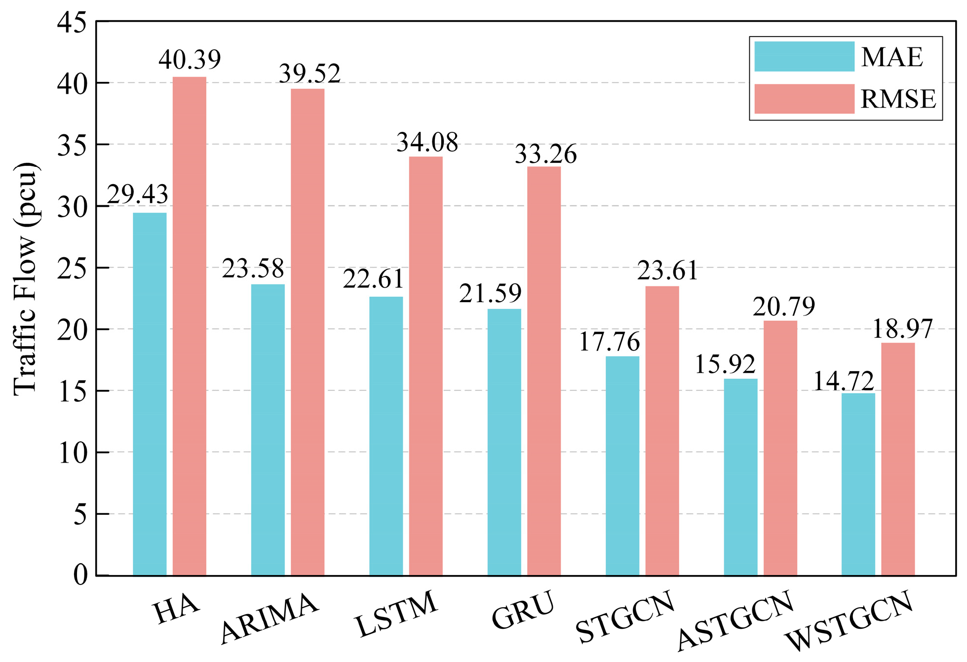
To objectively evaluate the performance of different models in predicting traffic flow for the next hour, mean absolute error (MAE) and root mean square error (RMSE) are used as metrics. The predictive performance of each model is shown in Figure 5.
From Figure 5, it is evident that the proposed WSTGCN model achieves the best prediction accuracy compared to other benchmark models. Also, it can be seen from the results that temporal models (HA, ARIMA, LSTM, and GRU) all perform poorer than the spatial–temporal models (STGCN, ASTGCN, and WSTGCN). This may be because temporal models only consider the temporal features inherent in the traffic data, but fail to capture the spatial correlation of traffic data at different nodes in the traffic network. Moreover, among the three spatial–temporal models, the proposed WSTGCN model performs the best. Compared to the second-best ASTGCN model, the WSTGCN model further reduces the MAE and RMSE by 7.5% and 8.6%. This is because the WSTGCN model not only integrates the attention mechanisms but also implements modified residual modules and employs a weight fusion mechanism to improve the fusion performance of recent, daily periodic and weekly periodic components. By fully exploiting the dynamic spatial–temporal correlations, the WSTGCN model subsequently enhances predictive accuracy in the traffic flow prediction task.

4.1.2. Ablation Study

To further validate the effectiveness of the modified residual modules and the introduced weight fusion in the WSTGCN model, ablation experiments are further conducted. To validate the modified residual modules, ASTGCN and the residual improved STGCN (RSTGCN) are compared. RSTGCN only incorporates the residual improvement module into ASTGCN but does not perform weight fusion. Moreover, RSTGCN and WSTGCN are compared to validate the effectiveness of the weight fusion, since WSTGCN further introduces the weight fusion mechanism based on the RSTGCN. Each model is used to predict traffic flow for the next hour, and MAE and RMSE are used as metrics.
From Figure 6, it can be seen that the WSTGCN has the best prediction performance, followed by the RSTGCN, and the ASTGCN is the poorest. Comparing RSTGCN and ASTGCN, the results indicate that the modified residual module with convolution operations is effective in enhancing the predicting accuracy of the ASTGCN. Moreover, comparing the WSTGCN and RSTGCN, the results demonstrate the effectiveness of the proposed weight fusion mechanism. By fully exploiting the interactions among recent, daily periodic, and weekly periodic components, the accuracy of the results can be further improved.

4.1.3. Predicting Performance under Different Predicting Horizons

To study the impact of predicting horizons on the performance of the predicting model, comparative experiments are conducted with prediction durations of 15 min, 30 min, and 1 h. The experimental results are shown in Table 1.
From Table 1, it can be seen that as the prediction duration increases, the difficulty of prediction also increases, leading to a decline in the predictive performance. Among all predicting horizons, the proposed WSTGCN model has the best predictive performance compared to other benchmark models, while the HA has the poorest performance. Also, it can be found that spatial–temporal deep learning models like STGCN, ASTGCN, RSTGCN, and WSTGCN outperform temporal models like HA, ARIMA, LSTM, and GRU. Additionally, the WSTGCN model performs better than the ASTGCN and RSTGCN, which indicates the effectiveness of the modified residual modules and the introduced weight fusion.

4.2. Charging Load Model Validation

Based on the traffic flow prediction results from the WSTGCN model, the charging load of FCS is further analyzed by the proposed improved queuing theory model. In the experiment, the maximum charging power of the FCS is set to P FCS max = 12 MW, and the total number of servers is set to C = 25, with each server providing a charging power of pch = 40 kW. The FCS can accommodate up to N = 30 EVs at a time, and the average charging time for an EV is 20 min. The probability parameters for refusal to join and impatience to leave are denoted as σ = 1 and δ = 1. Based on the total vehicle stock [28] and EV stock data [29], the penetration rate of EVs in the United States in 2020 was 2.2%, and the probability of an EV needing to charge at any given time is 20%.

4.2.1. Charging Load Prediction Results

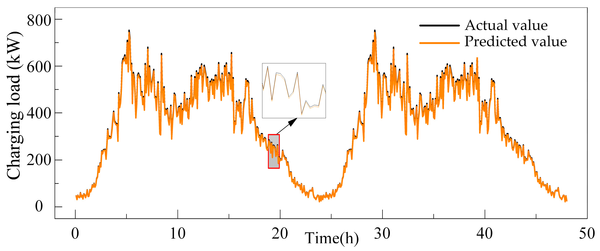
The charging load prediction results based on the improved queuing theory model are shown in Figure 7. It can be observed that the predicted charging load closely approximates the actual values, indicating that the improved queuing model is effective for predicting the charging load of FCSs.

4.2.2. Impact of the WSTGCN Model

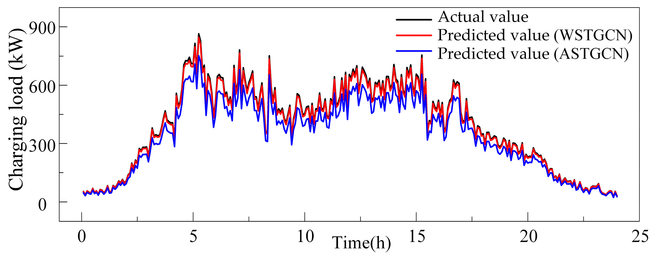
To validate the impact of the proposed WSTGCN model on the accuracy of charging load predictions, both the WSTGCN and benchmark ASTGCN models are used for traffic flow prediction. And then, based on the traffic flow prediction results, the improved queuing model is used to predict the charging load of FCS. The charging load prediction results are shown in Figure 8. To perform further quantitative analysis, the MAE and RMSE are selected as metrics to compare the prediction accuracy of the two models.
From Figure 8, it can be intuitively observed that the results of the WSTGCN-based charging load prediction model are closer to the actual values than those of the ASTGCN-based model. Moreover, from Table 2, it can be found that the WSTGCN-based traffic flow prediction model has better predictive performance compared to the benchmark ASTGCN model. These results indicate that the charging load prediction accuracy is influenced by the traffic flow prediction results significantly. More accurate traffic flow prediction results contribute to more accurate charging load prediction results. The improved WSTGCN provides more accurate traffic flow prediction results, thus greatly improving the accuracy of charging load prediction.

4.2.3. Impact of Improved Queuing Model

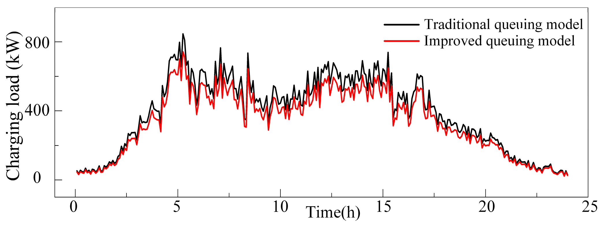
To validate the impact of the queuing model on charging load predictions, the improved queuing model and the traditional queuing model are both used to predict the charging load of FCS based on the same traffic flow prediction results from WSTGCN. The results are shown in Figure 9.
From Figure 9, it can be intuitively seen that the charging load predicted by the improved queuing theory model is lower than that of the traditional queuing theory model. This may be because the subjective behaviors of EV owners are fully considered in the improved queuing theory model, affecting the prediction results significantly. Due to the limited capacity of the FCSs, some EVs leave the FCS without receiving charging service, resulting in a loss of charging load.

4.2.4. Sensitivity Analysis

To explore the impact of key parameters on prediction results, sensitivity analyses are conducted for the number of servers C, the maximum capacity of the FCS N, the refusal to join intensity parameter σ, and the impatience to leave intensity parameter δ.
As shown in Figure 10a, when the number of servers C or the maximum capacity N increases, the predicted charging load correspondingly increases. This is because the limited capacity of the FCS significantly influences the EV arrival rate. If the service capacity of the FCS is small, charging servers will easily become fully occupied; thus, some EVs are forced to leave, resulting in a loss of charging load. The results indicate that the service capacity of the FCS deeply influences the charging behaviors of the EVs. The insufficient service capacity will limit the widespread use of EVs to some extent. Therefore, constructing adequate charging facilities can greatly facilitate EV charging and promote EV development.
Figure 10b shows the impact of the refusal parameter σ and the impatience parameter δ. The results show that if drivers are more sensitive to waiting times, reflected by a larger refusal parameter σ and impatience parameter δ, the charging load decreases accordingly. Additionally, it can be observed that the reduction in charging loads is particularly noticeable during peak periods. This is because, during the peak time, the number of queuing EVs increases, resulting in a larger leaving rate and lower arrival rate than other periods, thus leading to a larger loss in charging load.

4.2.5. Impact of FCS Scale on Service Performance

Through the analysis of the queuing model, the service performance of the FCS can be further assessed. This service performance is directly linked to user experience at the FCS, which is crucial for enhancing customer satisfaction and promoting the adoption of electric vehicles. We choose two metrics to quantify the service performance of different scale FCSs, i.e., average waiting time and average queue length of EVs. The results are shown in Figure 11.
From Figure 11, it can be found that the service performance of the FCS is directly related to its scale. As the number of charging servers C and the capacity N decrease, the average queue length and average waiting time for EVs increase. Additionally, it can be seen that when the scale of FCS exceeds 15 servers and can accommodate up to 20 EVs, the improvements in service performance become marginal. Therefore, it can be concluded that the installation of FCS should be planned for an optimal scale. If there are too few servers, service quality suffers, leading to excessively long wait times; conversely, if there are too many, the improvement in service quality is negligible while investment costs rise. The proposed model can effectively model the charging process and provide strategic insights for the planning of charging stations.

5. Conclusions

This paper proposes a deep learning-based model for predicting the charging load of FCSs to quantify the impact of EV charging on the power grid. The main work can be concluded as follows: (i) An improved WSTGCN model is proposed to model the EV traffic flow, considering the inherent spatial–temporal characteristics of traffic flow. Compared to temporal models (HA, ARIMA, LSTM, and GRU), the WSTGCN not only considers the temporal feature inherent in the traffic data, but also captures the spatial correlation of traffic data at different nodes in the traffic network. By fully exploiting the dynamic spatial–temporal correlations, the WSTGCN model performs much more accurately than temporal models. (ii) By modifying the residual modules and integrating the weight fusion mechanism into the WSTGCN model, the prediction performance has been significantly enhanced. The experimental results show that the proposed WSTGCN model exhibits superior accuracy in predicting traffic flow compared to other benchmark models. Compared to the second-best ASTGCN model, the WSTGCN model further reduces the MAE and RMSE by 7.5% and 8.6%. (iii) An improved queuing theory model is used to predict the EV charging load of FCSs with special consideration of subjective EV user behaviors. By considering the behaviors of EV users refusing to join and leaving impatiently, the predicted charging load of the FCS is lower than the traditional queuing theory model, especially during peak times. Additionally, it should be noted that the proposed charging load prediction method is based on traffic flow prediction, which can successfully address the challenge of lacking historical data, thus holding important practical value in charging load prediction for newly established FCSs.

Author Contributions

Conceptualization, J.Z. and H.C.; software, J.Z.; methodology, H.Z., Z.W. (Zhiqiang Wang) and Z.W. (Ziyi Wen); visualization, Z.W. (Ziyi Wen); writing—original draft, Z.W. (Ziyi Wen); formal analysis, X.Z.; supervision, X.Z.; writing—review and editing, X.Z. All authors have read and agreed to the published version of the manuscript.

Funding

This research was funded by the National Natural Science Foundation of China, grant number 72001058; Guangdong Basic and Applied Basic Research Foundation, grant numbers 2023A1515010724 and 2022A1515240051; General Program of Foundation of Shenzhen Science and Technology Committee, grant number GXWD20231130154831002; Major Science and Technology Special Projects in Xinjiang Autonomous Region, grant number 2022A01007; and Xinjiang Autonomous Region Key Research and Development Task Special Project, grant number 2022B01016.

Data Availability Statement

The contributions presented in the study are included in the article.

Conflicts of Interest

Author Jun Zhang, Huiluan Cong, Hui Zhou, Zhiqiang Wang were employed by the company State Grid Shandong Electric Vehicle Service Company Ltd. The remaining authors declare that the research was conducted in the absence of any commercial or financial relationships that could be construed as a potential conflict of interest.

References

  1. Amini, M.; Kargarian, A.; Karabasoglu, O. ARIMA-based decoupled time series forecasting of electric vehicle charging demand for stochastic power system operation. Electr. Power Syst. Res. 2016, 140, 378–390. [Google Scholar] [CrossRef]
  2. Louie, H.M. Time-series modeling of aggregated electric vehicle charging station load. Electr. Power Compon. Syst. 2017, 45, 1498–1511. [Google Scholar] [CrossRef]
  3. Akshay, K.C.; Grace, G.H.; Gunasekaran, K.; Samikannu, R. Power consumption prediction for electric vehicle charging stations and forecasting income. Sci. Rep. 2024, 14, 6497. [Google Scholar] [CrossRef] [PubMed]
  4. Wang, S.; Zhuge, C.; Shao, C.; Wang, P.; Yang, X.; Wang, S. Short-term electric vehicle charging demand prediction: A deep learning approach. Appl. Energy 2023, 340, 121032. [Google Scholar] [CrossRef]
  5. Yi, Z.; Liu, X.; Wei, R.; Chen, X.; Dai, J. Electric vehicle charging demand forecasting using deep learning model. J. Intell. Transp. Syst. 2022, 26, 690–703. [Google Scholar] [CrossRef]
  6. Jahangir, H.; Gougheri, S.; Vatandoust, B.; Golkar, M.A.; Ahmadian, A.; Hajizadeh, A. Plug-in electric vehicle behavior modeling in energy market: A novel deep learning-based approach with clustering technique. IEEE Trans. Smart Grid 2020, 11, 4738–4748. [Google Scholar] [CrossRef]
  7. Sasidharan, M.; Kinattingal, S.; Simon, S. Comparative analysis of deep learning models for electric vehicle charging load forecasting. J. Inst. Eng. Ser. B 2023, 104, 105–113. [Google Scholar] [CrossRef]
  8. Dabbaghjamanesh, M.; Moeini, A.; Kavousi-Fard, A. Reinforcement learning-based load forecasting of electric vehicle charging station using Q-learning technique. IEEE Trans. Ind. Inf. 2021, 17, 4229–4237. [Google Scholar] [CrossRef]
  9. Mekkaoui, D.; Midoun, M.; Shen, Y. LA-RCNN: Luong attention-recurrent-convolutional neural network for EV charging load prediction. Appl. Intell. 2024, 54, 4352–4369. [Google Scholar] [CrossRef]
  10. Li, Y.; Huang, Y.; Zhang, M. Short-term load forecasting for electric vehicle charging station based on niche immunity lion algorithm and convolutional neural network. Energies 2018, 11, 1253. [Google Scholar] [CrossRef]
  11. Wang, S.; Chen, A.; Wang, P.; Zhuge, C. Predicting electric vehicle charging demand using a heterogeneous spatio-temporal graph convolutional network. Transp. Res. Part C Emerg. Technol. 2023, 153, 104205. [Google Scholar] [CrossRef]
  12. Su, S.; Li, Y.; Chen, Q.; Xia, M.; Yamashita, K.; Jurasz, J. Operating status prediction model at EV charging stations with fusing spatiotemporal graph convolutional network. IEEE Trans. Transp. Electrif. 2023, 9, 114–129. [Google Scholar] [CrossRef]
  13. Chen, Y.; Wang, M.; Wei, Y.; Huang, X.; Gao, S. Multi-encoder spatio-temporal feature fusion network for electric vehicle charging load prediction. J. Intell. Robot. Syst. 2024, 110, 94. [Google Scholar] [CrossRef]
  14. Li, M.; Zhu, Z. Spatial-Temporal Fusion Graph Neural Networks for Traffic Flow Forecasting. Proc. AAAI Conf. Artif. Intell. 2021, 35, 4189–4196. [Google Scholar] [CrossRef]
  15. Li, F.; Feng, J.; Yan, H.; Jin, J.; Yang, F.; Sun, F.; Jin, D.; Li, Y. Dynamic graph convolutional recurrent network for traffic prediction: Benchmark and solution. ACM Trans. Knowl. Discov. Data 2023, 17, 1–21. [Google Scholar] [CrossRef]
  16. Zhang, Y.; Liu, C.; Rao, X.; Zhang, X.B.; Zhou, Y. Spatial-temporal load forecasting of electric vehicle charging stations based on graph neural network. J. Intell. Fuzzy Syst. 2024, 46, 821–836. [Google Scholar] [CrossRef]
  17. Shi, J.; Zhang, W.; Bao, Y.; Gao, D.W.; Wang, Z.H. Load forecasting of electric vehicle charging stations: Attention-based spatiotemporal multi-graph convolutional networks. IEEE Trans. Smart Grid 2023, 15, 3016–3027. [Google Scholar] [CrossRef]
  18. Zhang, X.; Chan, K.W.; Li, H.; Wang, H.; Qiu, J.; Wang, G. Deep-learning-based probabilistic forecasting of electric vehicle charging load with a novel queuing model. IEEE Trans. Cybern. 2020, 51, 3157–3170. [Google Scholar] [CrossRef]
  19. Wu, T.; Ji, X.; Wang, G.; Liu, Y.; Yang, Q.; Bao, Z.; Peng, J. Hydrogen energy storage system for demand forecast error mitigation and voltage stabilization in a fast-charging station. IEEE Trans. Ind. Appl. 2021, 58, 2718–2727. [Google Scholar] [CrossRef]
  20. Arias, M.B.; Kim, M.; Bae, S. Prediction of electric vehicle charging-power demand in realistic urban traffic networks. Appl. Energy 2017, 195, 738–753. [Google Scholar] [CrossRef]
  21. Feng, J.; Chang, X.; Fan, Y.; Luo, W. Electric vehicle charging load prediction model considering traffic conditions and temperature. Processes 2023, 11, 2256. [Google Scholar] [CrossRef]
  22. Tang, S.; Mu, Y.; Zhou, Y.; Dong, X.; Jia, H. A spatial-temporal electric vehicle charging load forecasting method considering the coordination among the multiple charging behaviors. In Proceedings of the 2021 Power System and Green Energy Conference (PSGEC), Shanghai, China, 20–22 August 2021; pp. 629–634. [Google Scholar]
  23. Guo, S.; Lin, Y.; Feng, N.; Song, C.; Wan, H. Attention-based spatial-temporal graph convolutional networks for traffic flow forecasting. Proc. AAAI Conf. Artif. Intell. 2019, 33, 922–929. [Google Scholar] [CrossRef]
  24. Williams, B.M.; Hoel, L.A. Modeling and forecasting vehicular traffic flow as a seasonal ARIMA process: Theoretical basis and empirical results. J. Transp. Eng. 2003, 129, 664–672. [Google Scholar] [CrossRef]
  25. Sutskever, I.; Vinyals, O.; Le, Q.V. Sequence to sequence learning with neural networks. arXiv 2014, arXiv:1409.3215. [Google Scholar]
  26. Chung, J.; Gulcehre, C.; Cho, K.H.; Bengio, Y. Empirical evaluation of gated recurrent neural networks on sequence modeling. arXiv 2014, arXiv:1412.3555. [Google Scholar]
  27. Yu, B.; Yin, H.; Zhu, Z. Spatio-temporal graph convolutional networks: A deep learning framework for traffic forecasting. arXiv 2017, arXiv:1709.04875. [Google Scholar]
  28. Our World in Data. Number of New Cars Sold, by Type, World. Available online: https://ourworldindata.org/energy (accessed on 18 September 2024).
  29. IEA. Global Electric Car Stock, 2013–2023. Available online: https://www.iea.org/data-and-statistics/charts/global-electric-car-stock-2013-2023 (accessed on 18 September 2024).
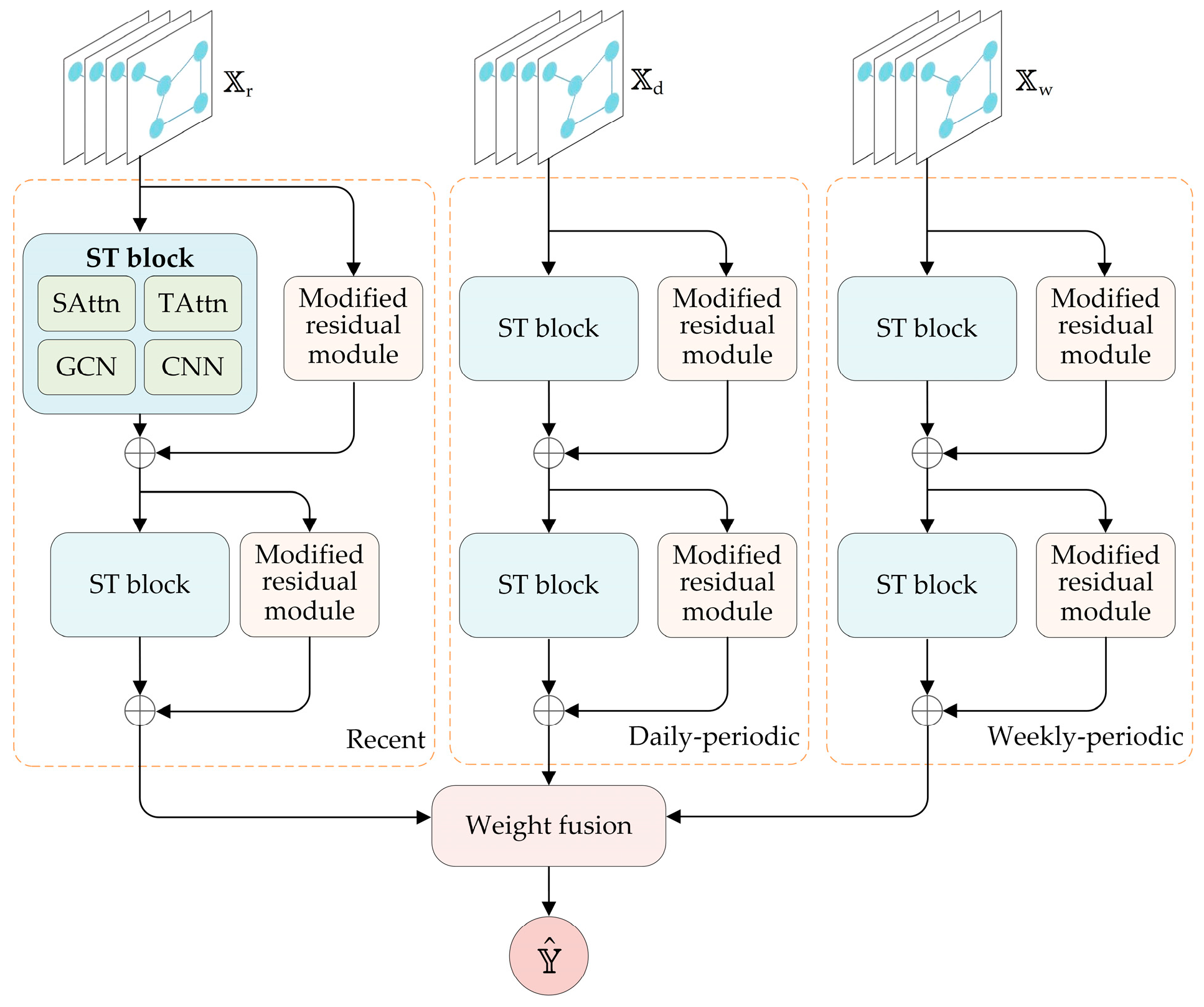
Figure 1. WSTGCN model.
Energies 17 04798 g001
Figure 2. ST block.
Figure 2. ST block.
Energies 17 04798 g002
Figure 3. Weight fusion mechanism.
Energies 17 04798 g003
Figure 4. State transition of the improved queueing model.
Energies 17 04798 g004
Figure 5. Predictive performance of different models.
Energies 17 04798 g005
Figure 6. Performance of ASTGCN, RSTGCN, and WSTGCN.
Energies 17 04798 g006
Figure 7. The prediction results of charging load.
Energies 17 04798 g007
Figure 8. The prediction results of different models.
Energies 17 04798 g008
Figure 9. The charging load prediction results.
Energies 17 04798 g009
Figure 10. (a) The impact of parameters C and N; (b) the impact of parameters σ and δ.
Energies 17 04798 g010
Figure 11. (a) Average waiting time; (b) average queue length.
Energies 17 04798 g011
Table 1. Performance comparison of different predicting horizons.
Predicting HorizonMetrixHAARIMALSTMGRUSTGCNASTGCNRSTGCNWSTGCN
15 minMAE23.1518.3316.8916.2515.0312.4512.1511.04
RMSE35.9629.4926.7225.9120.1218.6918.2416.54
30 minMAE26.5419.7719.9319.4716.8514.5114.1613.25
RMSE38.1736.9130.2929.8422.3719.5819.1117.63
1 hMAE29.4323.5822.6121.5917.7615.9215.5614.72
RMSE40.3939.3234.0833.2623.6120.7920.3618.97
Table 2. Performance comparison of different traffic flow prediction models.
Traffic Flow ModelASTGCNWSTGCN
Charging modelImproved queuing model
MAE15.329.01
RMSE17.7610.47
Disclaimer/Publisher’s Note: The statements, opinions and data contained in all publications are solely those of the individual author(s) and contributor(s) and not of MDPI and/or the editor(s). MDPI and/or the editor(s) disclaim responsibility for any injury to people or property resulting from any ideas, methods, instructions or products referred to in the content.