A 24-Step Short-Term Power Load Forecasting Model Utilizing KOA-BiTCN-BiGRU-Attentions

Abstract

With the global objectives of achieving a “carbon peak” and “carbon neutrality” along with the implementation of carbon reduction policies, China’s industrial structure has undergone significant adjustments, resulting in constraints on high-energy consumption and high-emission industries while promoting the rapid growth of green industries. Consequently, these changes have led to an increasingly complex power system structure and presented new challenges for electricity demand forecasting. To address this issue, this study proposes a 24-step multivariate time series short-term load forecasting algorithm model based on KNN data imputation and BiTCN bidirectional temporal convolutional networks combined with BiGRU bidirectional gated recurrent units and attention mechanism. The Kepler adaptive optimization algorithm (KOA) is employed for hyperparameter optimization to effectively enhance prediction accuracy. Furthermore, using real load data from a wind farm in Xinjiang as an example, this paper predicts the electricity load from 1 January to 30 December in 2019. Experimental results demonstrate that our comprehensive short-term load forecasting model exhibits lower prediction errors and superior performance compared to traditional methods, thus holding great value for practical applications.

1. Introduction

Load forecasting is a crucial prerequisite for maintaining a power system’s dynamic balance between supply and demand. Its accuracy significantly impacts the power system’s planning, operation, and economic dispatching. As a core technology in the power system, load forecasting plays a vital role in ensuring power supply stability, optimizing resource allocation, and assisting decision-making. With the robust development of the global power market, the complexity and dynamics of the power system are escalating. The integration of various distributed new energy sources, the emergence of the new interaction mode of “source-network-charge-storage”, and the pursuit of the power industry to enhance quality and efficiency have imposed higher demands for load forecasting accuracy. Against this backdrop, the continuous improvement and optimization of load forecasting technology have become vital to auxiliary power supply decision-making and maintaining power system stability.

The composition of the load in the force system is relatively straightforward and the prediction scenario is primarily focused on the system level or bus bar due to the traditional electrical level. As a result, the conventional method of load prediction is a relatively simple statistical analysis-based approach. Examples of such models include the linear regression model and the Holt-Winters model [1,2]. While these models are easy to derive and interpret, their generalization capabilities are limited. With the rapid growth of the power system, particularly the development of new power systems, numerous new elements have been introduced, such as distributed renewable energy and electric vehicles, significantly increasing the uncertainty of the load side of the power system. Concurrently, due to the increasing popularity of demand-side management, new roles have emerged, such as producers and consumers, load aggregators, etc., leading to a more active interaction between users and the grid. In light of these complex load factors, it can be observed that the traditional load forecasting methods struggle to construct the load model accurately in the context of new power systems.

To address this issue, data-driven artificial intelligence has progressively emerged as the primary application approach and research direction for power system load forecasting. At present, AI-based methods can be primarily categorized into traditional machine learning techniques and deep learning methods. Prediction approaches relying on conventional machine learning often encompass random forest algorithm [3], decision tree regression [4], gradient lifting tree (GBDT) regression [5], CatBoost regression [6], support vector regression (SVR) [7], extreme gradient boost (XGBoost) [8], and extreme learning machine (ELM) [9], among others. These methods exhibit significant advantages when addressing nonlinear problems. Nonetheless, challenges such as complex data correlation processing, multiple feature dimensions, vast data scales, and slow processing speeds [10] still persist. The deep learning method, on the other hand, can extract hidden abstract features layer by layer from a vast amount of data through multilayer nonlinear mapping, thereby effectively enhancing prediction efficacy. Among various neural networks, the recurrent neural network (RNN) demonstrates effectiveness in addressing wind power prediction-related issues. However, traditional backpropagation neural networks are susceptible to falling into local optimal solutions, leading to gradient disappearance and gradient explosion [10]. To overcome this issue, long short-term memory (LSTM) and gated recurrent unit (GRU) networks introduce unique unit structures to the basic RNN [11,12], making them increasingly applicable to wind speed and wind power prediction. The integration of random forest and LSTM neural network was proposed in the literature [13] for power load prediction, yielding satisfactory results. The literature [14] introduced an algorithm based on a multivariable short-duration memory network (MLSTM) to exploit historical wind power and wind speed data for more accurate wind power forecasting, demonstrating stable performance across different datasets. Temporal convolutional neural networks (TCN) built upon convolutional neural networks (CNNS) were also explored, with the convolutional architecture proven to excel over typical cyclic networks across various tasks and data sets, while the flexible, sensitive field exhibited a longer adequate memory. The literature [15] enhanced the CNN-LSTM model to predict ultra-short-term offshore wind power, implementing an optimal combination of attention-strengthening and spatial characteristic weak modules to boost wind power output reliability. GRU, an LSTM derivative, simplified the neural unit structure and boasted a faster convergence rate. The literature [16] proposed the prediction of low- and high-frequency data using multiple linear regression and GRU neural networks, respectively, and combined the outcomes from each to generate the final prediction. Lastly, the literature [17] merged CNN-GRU, extracting multidimensional load influencing factors through CNN before constructing a feature vector in the form of a time series to be used as the input for the GRU network, thoroughly investigating the dynamic change rule characteristics within the data.

Through an in-depth exploration of machine learning algorithms in load prediction, researchers can select various network models for this purpose and choose the most suitable model algorithm that can significantly enhance the accuracy of load prediction. However, setting hyperparameters in network models through manual experience is both inconvenient and challenging. Consequently, numerous advanced intelligent optimization algorithms have been extensively employed in load forecasting to aid network models in determining appropriate network parameters, thereby improving the accuracy of load forecasting. In recent years, scholars have conducted mathematical simulations to analyze the survival strategies, evolutionary processes, and competitive mechanisms of various creatures in nature as well as the formation, development, and termination of natural phenomena. Additionally, they have examined the relationship between matter and the method of inquiry in natural and human sciences, resulting in the proposal of numerous ROAs. In 1988, Professor Holland, inspired by the biological evolution found in nature, introduced the genetic algorithm (GA) [18], laying the groundwork for the development of advanced intelligence algorithms. Building on the collective behavior of biological groups in nature, Eberhart and his colleagues advanced the particle swarm optimization algorithm (PSO) in 1995 [19], followed by Dorigo et al., who proposed the ant colony algorithm (ACO) [20]. Additionally, algorithms based on physical principles, such as the gravitational search algorithm (GSA) proposed by Rashedi et al. in 2009 [21], and those inspired by human social behavior, such as the instructional learning optimization algorithm (TLBO) proposed by Rao et al. in 2011 [22], were also developed. In the evolution of stochastic optimization algorithms, researchers continuously put forward new methods based on the “No Free Lunch Theorem” (NFL) [23]. The NFL asserts that no learning algorithm is universally superior to all others without prior assumptions regarding the problem domain. This implies that the average performance of all algorithms is identical across all possible problems. This theorem emphasizes the significance of considering specific problem characteristics when selecting a learning algorithm. This also further boosts the performance of existing methods. Notable examples include the marine predator algorithm (MPA) [24], chameleon algorithm (CSA) [25], Archimedes optimization algorithm (AOA) [26], golden eagle optimization algorithm (GEO) [27], Stochastic Frank-Wolfe (SFO) [28], chimp optimization algorithm (ChOA) [29], slime bacteria algorithm (SMA) [30], and dandelion optimization algorithm (DO) [31], African vulture optimization algorithm (AVOA) [32], aphid–ant mutualism algorithm (AAM) [33], beluga optimization algorithm (BWO) [34], elephant clan optimization algorithm (ECO) [35], human happiness algorithm (HFA) [36], and gander optimization algorithm (GOA) [37]. These methods are extensively employed to enhance the precision of relevant load forecasting techniques. For instance, in reference [38], the CSA optimization algorithm is used to improve the load prediction accuracy of DBN-SARIMA. Similarly, reference [39] leverages the GOA algorithm to optimize the accuracy of LSSVR load prediction. Among these, the Kepler optimization algorithm (KOA) [40] is a novel optimization method based on a physical model proposed by Abdel-Basset et al. in 2023. It exhibits a significant improvement in performance compared to previous optimization algorithms.

In the process of handling load data summaries, it is unavoidable that vacant data will occasionally occur. To ensure the continuity of the data and the comprehensiveness of the features, it is crucial to fill in these gaps. The traditional filling methods can be categorized into statistical-based approaches and machine-learning-based approaches. The statistical techniques primarily include mean filling, conditional mean filling, and global constant filling. At present, machine-learning-based methods mainly encompass decision-tree-based filling [41] and neural network regression-based loading [42]. Notably, several statistical methods fail to identify the correlation between the data effectively, resulting in shortcomings regarding the accuracy of filling vacant values. Conversely, several machine-learning-based methods, to some extent, take into account the correlation between the data, thereby exhibiting better performance compared to their statistical counterparts. However, these methods are generally effective only for linear and noise-free data sets. With the progression of information acquisition technology, humans are confronted with a multitude of nonlinear noise data sets. Consequently, the development of high-performance gap-filling algorithms for such nonlinear noise data sets holds significant research value. Among these algorithms, the KNN (K-nearest neighbors) approach, being a relatively novel method, demonstrates excellent nonlinear data fitting performance and exhibits robust resistance to noise interference in tests.

The attention mechanism is a model proposed by Treisman and Gelade to simulate the attention mechanism of the human brain [43]. The emergence of this model has addressed the deficiencies of recurrent neural networks in processing long sequences, such as gradient vanishing and computational inefficiency. Its innovation and application effects have sparked great interest, leading to the proposal of many related models in the past few years. These models have achieved significant success in various artificial intelligence fields such as large language models, computer vision, and audio processing. The attention mechanism exhibits strong modeling capabilities for long-range dependencies and interactions in sequential data, making it highly attractive for time series modeling. Ref. [44] employs a convolutional self-attention mechanism, which incorporates local information into the attention mechanism through causal convolutions and uses a sparse attention strategy to reduce computational complexity. Model [45] adopts a sparse transformer as a generator to learn sparse attention maps for time series prediction and uses a discriminator at the sequence level to improve prediction performance. Ref. [46] achieves logarithmic time complexity and memory overhead through methods such as the prob-sparse self-attention mechanism and a generative decoder, enabling one-time prediction of long time series. Ref. [47] sets time series decomposition as an internal module of deep neural networks and designs an autocorrelation mechanism based on periodicity to discover and represent time series dependencies. Ref. [48] introduces a pyramidal attention module, where the tree structure between scales summarizes features of different resolutions, while adjacent connections within the same scale model time dependencies of different ranges. Ref. [49] proposes a frequency-enhanced transformer method that combines the sparse representation of time series Fourier transforms to capture detailed structures of time series data while using decomposition methods to capture global information. Ref. [50] employs a data segmentation approach to embed the input multivariate time series into a 2D vector to preserve both time and dimension information and then uses a two-stage attention layer to capture cross-time and cross-dimension dependencies.

In summary, this paper proposes a novel method founded on KNN data-filling processing. The BiTCN (bidirectional time convolutional) network is optimized utilizing the Kepler adaptive optimization algorithm (KOA). This study presents a 24-step multivariable time series short-term load regression prediction algorithm, which is based on a bidirectional time convolutional network integrated with a bidirectional gated cycle unit (BiGRU) and attention mechanism. By incorporating power load influencing factors, such as electricity price, load, weather, and temperature, the model trains on a multitude of historical data, extracting and mapping the internal relationship between input and output, ultimately achieving accurate prediction results. During the experiment, the KNN model was utilized to fill in missing values. Subsequently, the feature data were fed into the BiTCN and BiGRU models, where their time series modeling capabilities, in conjunction with the bidirectional context capture and attention to crucial information, were harnessed. This approach capitalized on the strengths of each model, extracting features at different levels and dimensions and merging them. Finally, the attention mechanism was employed to weigh various features based on their respective importance at additional time steps, thereby calculating the attention weight for each time step and facilitating the ultimate prediction. Experimental results indicate that, in comparison to traditional methods, the proposed approach presents a lower prediction error and superior model performance, thus demonstrating a more comprehensive range of application values.

2. Related Methodologies

2.1. Load Type Classification

The load forecasting can be categorized into long-term, short-term, and medium-term load forecasting based on the duration. This is primarily utilized to facilitate power supply and grid infrastructure planning or to develop long-term operation and maintenance strategies. Short-term load forecasting offers valuable insights for daily production planning, frequency modulation unit adjustments, and more, thereby contributing significantly to ensuring the safe and stable operation of the power grid in real time.

2.2. KOA Optimization Algorithm

The Kepler optimization algorithm is a heuristic optimization algorithm proposed by Abdel-Basset et al. [40]. In the KOA, the sun and the planets rotating around the sun in elliptical orbits can be used to represent the search space. Since the positions of the planets (the candidate solutions) relative to the sun (optimal solution) change over time, the search space can be explored and utilized more efficiently. During the optimization process, the KOA will apply the following rules:

(1)

The orbital periods of planets (the candidate solutions) are randomly selected from a normal distribution.

(2)

The eccentricity of planets (the candidate solutions) is generated randomly within the range of [0,1].

(3)

The fitness of each solution is calculated based on the objective function.

(4)

In the iterative process, the best solution serves as the central star (sun).

(5)

Planets move around the sun in elliptical orbits, resulting in changes in their distance over time.

Based on the above rules, after evaluating the fitness of the initial set, the KOA runs iteratively until a termination criterion is met. Theoretically, the KOA can be regarded as a global optimization algorithm due to its exploration and exploitation phases. The following is a detailed description of the KOA’s iterative process from a mathematical point of view.

Step 1. Initial process:

The population size, denoted as N in this process, will be randomly distributed in d dimensions according to Formula (1), representing the decision variables of an optimization problem.

$${\theta }_g^i={\theta }_{g,low}^i+rand[0,1]\times ({\theta }_{g,up}^i+{\theta }_{g,low}^i)\{\begin{array}{l}i=1,2,\dots ,N\hfill \\ g=1,2,\dots ,d\hfill \end{array}$$

(1)

where ${\theta }_g^i$ denotes the g-th planet (candidate solution) in the search space, it represents the number of candidate solutions in the search space; ${\theta }_g^i$ represents the dimension of the problem to be optimized; ${\theta }_{g,up}^i$ ${\theta }_g^i$ represents the dimension of the problem to be optimized; ${\theta }_{g,up}^i$ and ${\theta }_{g,low}^i$ denote the upper and lower bounds of the g-th decision variable, respectively; and $rand\left[\mathrm{0,1}\right]$ denotes a randomly generated number at [0,1].

The g-th planet (candidate solution) in the search space is denoted by ${\theta }_g^i$, where $N$ represents the total number of candidate solutions in the search space. The dimension of the problem to be optimized is represented by $d$. ${\theta }_{g,up}^i$ and ${\theta }_{g,low}^i$ denote the upper and lower bounds of the g-th decision variable, respectively. Additionally, $rand\left[\mathrm{0,1}\right]$ represents a randomly generated number within the range [0,1].

For each object’s orbital eccentricity (e), it is initialized as in Formula (2):

$$e_i=rand[0,1]\hspace{1em}i=1,\dots ,N$$

(2)

where $rand[0,1]$ is a randomly generated number whose value ranges from [0,1].

Finally, for the orbital period of each planet (candidate solution), it is initialized as Formula (3):

$$T_i=\left|\begin{array}{c}r\end{array}\right|\hspace{1em}i=1,\dots ,N$$

(3)

where $r$ is a randomly generated number according to a normal distribution.

Step 2. Define the force of gravity (F):

The law of universal gravitation gives the gravitational pull of the sun ${\theta }_s$ and any planet ${\theta }_g$. Gravity is defined as Formula (4):

$$F_{gi}(t)=e\times \gamma (t)\times {\displaystyle \frac{M_s\times m_i}{{\overline{R_i}}^2+𝜕}}+r_1$$

(4)

In the formula for gravitation, $𝜕$ is a small number; $\gamma$ is the cosmological gravitational constant; e is the eccentricity of planetary orbits, whose value ranges from [0,1], which can give the KOA model more random features; $r_1$ is a randomly generated value between [0,1], which can provide more variation in the optimization process; ${\overrightarrow{R}}_i$ are the normalized value of $R_i$, which offers the Euclidean distance between the sun ${\theta }_s$ and the planets ${\theta }_g$, which is defined as Formula (5):

$$R_i(t)={\Vert {\theta }_s(t)-{\theta }_j(t)\Vert }_2=\sqrt{{\displaystyle \sum _{i=1}^d{\left[{\theta }_{sj}(t)-{\theta }_{ij}(t)\right]}^2}}$$

(5)

where ${‖{\theta }_s\left(t\right)-{\theta }_j\left(t\right)‖}_2$ offers the Euclidean distance between the sun’s dimensions and the planets’ dimensions ${\theta }_g$. The masses of the sun ${\theta }_s$ and the planets ${\theta }_g$ at time $t$ can be calculated using the following Formulas (6) and (7):

$$M_s=r_2{\displaystyle \frac{fi{t}_s(t)-worst(t)}{{\sum }_{\begin{array}{c}k=1\end{array}}^N[fi{t}_k(t)-worst(t)]}}$$

(6)

$$m_i={\displaystyle \frac{fi{t}_i(t)-worst(t)}{{\sum }_{\begin{array}{c}k=1\end{array}}^N[fi{t}_k(t)-worst(t)]}}$$

(7)

where the functions $fi{t}_s\left(t\right)$ and $worst\left(t\right)$ are defined as Formulas (8) and (9):

$$fi{t}_s(t)=best(t)=\underset{k\in 1,2,\dots ,N}{\min }fi{t}_k(t)$$

(8)

$$worst(t)=\underset{k\in 1,2,\dots ,N}{\max }fi{t}_k(t)$$

(9)

In the definition of solar mass $M_s$, a random constant $r_2$ from 0 to 1 is generated to represent the planet’s mass value within the scatter search space. The function $\gamma \left(t\right)$, which decreases exponentially with time to control the search accuracy, is defined as Formula (10):

$$\gamma \left(t\right)={\gamma }_0 \times \exp (-\varsigma {\displaystyle \frac{t}{T_{\max }}})$$

(10)

where $\varsigma$ is a constant; ${\gamma }_0$ is an initial value, while $t$ and $T_{\mathrm{m}\mathrm{a}\mathrm{x}}$ are the current iteration number and the maximum iteration number, respectively.

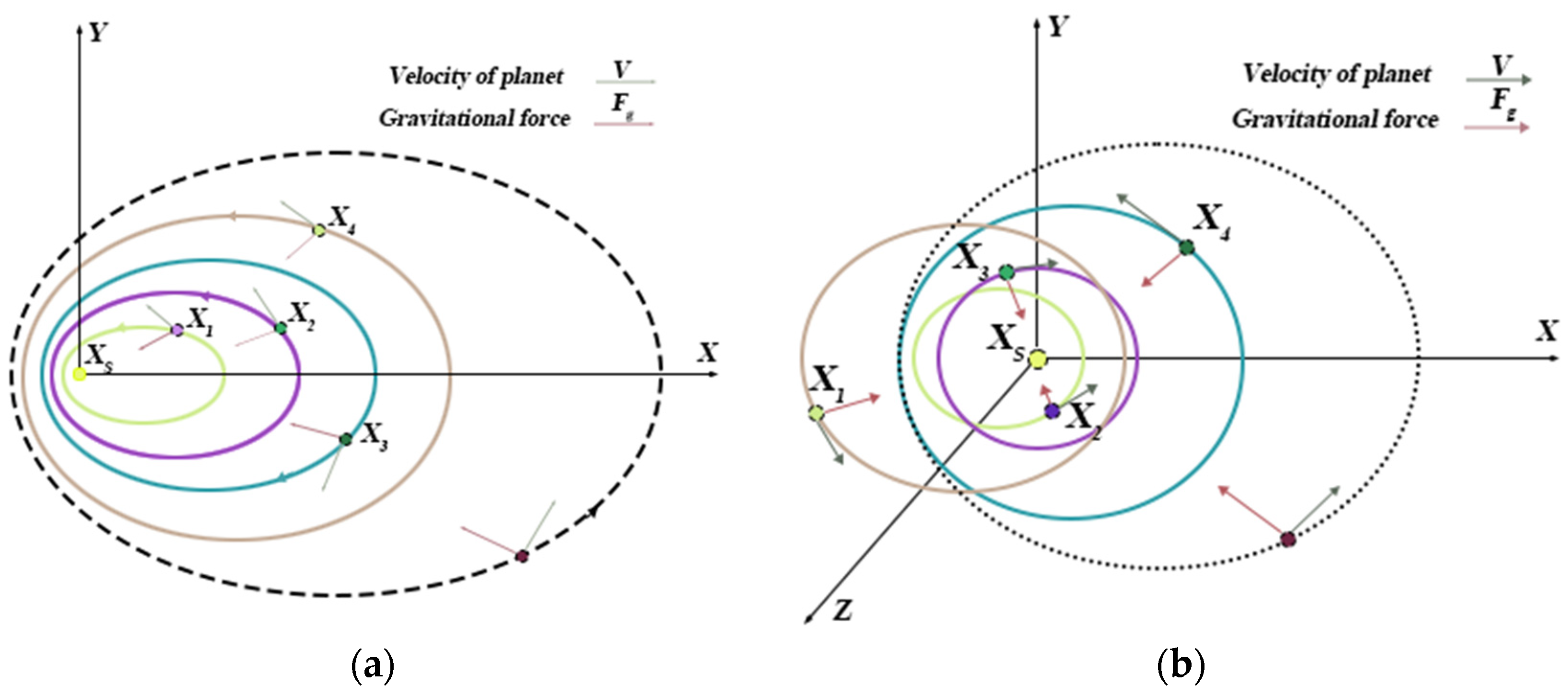
The specific motion is shown in Figure 1.

Figure 1. Possible positions in (a) 2-dimension and (b) 3-dimension.

Step 3. Calculate the planet’s velocity:

The planetary velocity depends on its setting relative to the sun ${\theta }_s$, and the closer you are to the sun ${\theta }_s$, the greater the velocity; the further away from the sun ${\theta }_s$, the slower it will be. This is understood to mean that as the gravity of the sun ${\theta }_s$ tries to capture the planet ${\theta }_g$, the planet ${\theta }_g$ increases its speed to avoid being pulled closer and slows down as it escapes. Mathematically, it is understood as the process of the KOA escaping from a local optimum solution, which can be described by the following Formulas (11)–(20):

$${\nu }_i(t)=\{\begin{array}{l}\sigma \times (2r_4\overrightarrow{{\theta }_{\mathrm{g}}}-\overrightarrow{{\theta }_h})+\ddot{\sigma }\times (\overrightarrow{{\theta }_g}-\overrightarrow{{\theta }_h})+[1-R_{g-norm}(t)]\hfill \\ \times \lambda \times \overrightarrow{W_1}\times \overrightarrow{r_5}\times (\overrightarrow{{\theta }_{g,up}}-\overrightarrow{{\theta }_{i,lov}}),if R_{G-\mathrm{nom}}(t)\le 0.5\hfill \\ r_4\times ℰ\times (\overrightarrow{{\theta }_a}-\overrightarrow{{\theta }_g})+[1-R_{g-norm}(t)]\hfill \\ \times \lambda \times \overrightarrow{W_2}\times \overrightarrow{r_5}\times (\overrightarrow{r_3({\theta }_{g,up}}-\overrightarrow{{\theta }_{i,lov}}),Else\hfill \end{array}$$

(11)

$$\sigma =\overrightarrow{U}\times \nu \times \epsilon$$

(12)

$$\epsilon ={\left[u(t)\times (M_s+m_g)\left|{\displaystyle \frac{2}{R_i(t)-\epsilon }}-{\displaystyle \frac{1}{a_{i(t)}+\epsilon }}\right|\right]}^{{\displaystyle \frac{1}{2}}}$$

(13)

$$\nu =[r_3\times (1-r_4)+r_4]$$

(14)

$$\overrightarrow{U}=\{\begin{array}{ll}0\hfill & \overrightarrow{r_5}\le \overrightarrow{r_4}\hfill \\ 1\hfill & else\hfill \end{array}$$

(15)

$$\lambda =\{\begin{array}{ll}1\hfill & \overrightarrow{r_5}\le \overrightarrow{r_4}\hfill \\ -1\hfill & else\hfill \end{array}$$

(16)

$$\ddot{\sigma }=(1-\overrightarrow{U})\times \upsilon \times \epsilon$$

(17)

$$\overrightarrow{\nu }=[r_3\times (1-\overrightarrow{r_5})+\overrightarrow{r_5}]$$

(18)

$$\overrightarrow{U_1}=\{\begin{array}{ll}0\hfill & \stackrel{\rightharpoonup }{r_5}\le \stackrel{\rightharpoonup }{r_4}\hfill \\ 1\hfill & else\hfill \end{array}$$

(19)

$$\overrightarrow{U_2}=\{\begin{array}{ll}0\hfill & \overrightarrow{r_3}\le \overrightarrow{r_4}\hfill \\ 1\hfill & else\hfill \end{array}$$

(20)

where the velocity of the planet ${\theta }_g$ at a given time is represented by ${\nu }_i\left(t\right)$, while ${\theta }_g$ represents the planet $g$. $r_3$ and $r_4$ are randomly generated numbers within the range [0,1], while $r_5$ and $r_6$ are random vectors contained in [0,1]. $\overrightarrow{{\theta }_g}$ and $\overrightarrow{{\theta }_h}$ represent a randomly selected solution from the population. $M_s$ and $m_g$ denote the masses of the sun ${\theta }_s$ and planets, respectively; $\mu \left(t\right)$ refers to the universal gravitational constant, while $\epsilon$ is a small value used to prevent division errors caused by zero frequency. $R_i\left(t\right)$ denotes the distance between the optimal solution ${\theta }_s$ and the object ${\theta }_g$ at a specific time. $a_i$ represents the semimajor axis of the planet ${\theta }_g$’s elliptical orbit at that time, which is defined by Kepler’s third law as shown in the following Formula (21):

$$a_g(t)=r_3\times {[T_g^2\times {\displaystyle \frac{\gamma (t)\times (M_s+m_g)}{4{\pi }^2}}]}^{{\displaystyle \frac{1}{3}}}$$

(21)

where $T_g$ denotes the orbital period of the planet $g$. In our proposed algorithm, it is assumed that the semimajor axis of the elliptical orbit of the planet ${\theta }_g$ gradually decreases with time. That is, its solution moves toward the region where the global optimal solution is expected to be found. $R_{g-norm}\left(t\right)$ denotes the Euclidean distance between the normalized $R_g$ and $R_s$, which is defined as Formula (22):

$$R_{g-norm}(t)={\displaystyle \frac{R_g(t)-min(R(t))}{max(R(t))-min(R(t))}}$$

(22)

The purpose of $R_{g-norm}\left(t\right)$ is to calculate the percentage of time steps each object will change. If $R_{g-norm}\left(t\right)\le 0.5$, the object is close to the sun and will increase its speed to prevent drifting toward the sun due to its huge gravitational pull. Otherwise, the planet $g$ will slow down.

Step 4. Escape the local optimum solution:

In the solar system, most objects rotate on their own axis while rotating counterclockwise around the sun ${\theta }_s$; however, some objects do the opposite, rotating clockwise around the sun. The KOA mimics this mechanism by using this behavior to escape the local algorithm optimal region, which is mainly embodied by a sign F that changes the search direction, thus giving the agent a good chance to scan the search space accurately.

Step 5. Update the object position:

Based on the previous section, the planet will rotate in an elliptical orbit around the sun. During this process, the object will move closer to the sun for some time and away from it. The KOA simulates this behavior mainly using two phases: exploration and exploitation. The KOA will explore objects far from the sun to find new solutions and, more accurately, find the optimal solution. In this way, the exploration and exploitation area around the sun is expanded. In the exploration phase, the target is far away from the sun (the optimal solution) and the whole search area can be explored more effectively. The target distance from the sun is the global optimal solution.

The position update formula is as Formula (23):

$${\overrightarrow{\theta }}_g(t+1)={\overrightarrow{\theta }}_g(t)+\lambda \times {\overrightarrow{V}}_g(t)+(F_{gi}(t)+|r|)\times \overrightarrow{U}\times ({\overrightarrow{\theta }}_s(t)-{\overrightarrow{\theta }}_g(t))$$

(23)

where ${\overrightarrow{\theta }}_g(t+1)$ is the new position of the object $g$ in time $t+1$, ${\overrightarrow{V}}_g(t)$ is the speed needed for the planet $g$ to reach the new position, ${\overrightarrow{\theta }}_s(t)$ is the best position of the sun found so far, and $\lambda$ is used as a sign to change the direction of the search. The position update formula simulates the gravitational force exerted by the sun on the planets. In this formula, a time step is introduced based on the calculation of the distance between the current planet and the sun, multiplied by the gravity of the sun. This modification aids the KOA in exploring its surrounding area after initialization, facilitating more efficient searches for optimal solutions with fewer function evaluations. In general, when the planet is moving away from the sun, the velocity of the planet will represent the KOA’s exploration operator. However, this speed is affected by the sun’s gravitational pull, which contributes to the region around the current better optimal solution for the planet. At the same time, as a planet approaches the sun, its speed will increase dramatically, allowing it to escape the sun’s gravitational pull. In this case, if the sun (the optimal solution) is the local minimum, the velocity represents the local optimal avoidance while the sun’s gravitational representation helps the KOA attack the best solution so far to find a better solution.

Step 6. Update the position with the sun:

If the distance between the sun and the planet is infinitesimally small, then either the planet or the sun emerges as the optimal solution during iterative processes.

This principle is randomly swapped with the formula. The position update formula further improves the KOA’s exploration operator, as shown in Step 5. The mathematical model of the principle is described as Formula (24):

$${\overrightarrow{\theta }}_i(t+1)={\overrightarrow{\theta }}_i(t)\times {\overrightarrow{U}}_1+(1-{\overrightarrow{U}}_1)\times ({\displaystyle \frac{{\overrightarrow{\theta }}_g(t)+{\overrightarrow{\theta }}_s+{\overrightarrow{\theta }}_a(t)}{3.0}}+h\times ({\displaystyle \frac{{\overrightarrow{\theta }}_g(t)+{\overrightarrow{\theta }}_s+{\overrightarrow{\theta }}_a(t)}{3.0}}-{\overrightarrow{\theta }}_b(t))$$

(24)

where $h$ is an adaptive factor that controls the distance between the sun and the current planet at the time $t$, which is defined as Formula (25):

$$h={\displaystyle \frac{1}{e^{\eta r}}}$$

(25)

where $r$ is a randomly generated number according to a normal distribution and $\eta$ is a [−2, 1] linear decreasing factor, defined as Formula (26):

$$\eta =(a_2-1)\times r_4+1$$

(26)

where $a_2$ is a cyclic control parameter and gradually reduced from −2 to −1 throughout the optimization process with period $T$ as Formula (27):

$$a_2=-1-1\times ({\displaystyle \frac{t\%\frac{T_{max}}{T}}{\frac{T_{max}}{T}}})$$

(27)

Step 7. Adjust the parameters:

This step implements an elite strategy to ensure the best placement of the planets and sun. Formula (28) summarizes the process:

$${\overrightarrow{\theta }}_{g,new}(t+1)=\{\begin{array}{l}{\overrightarrow{\theta }}_g(t+1),if (f({\overrightarrow{\theta }}_{g,new}(t+1))\le f({\overrightarrow{\theta }}_g(t)))\\ {\overrightarrow{\theta }}_g(t)\hspace{1em} Else \end{array}$$

(28)

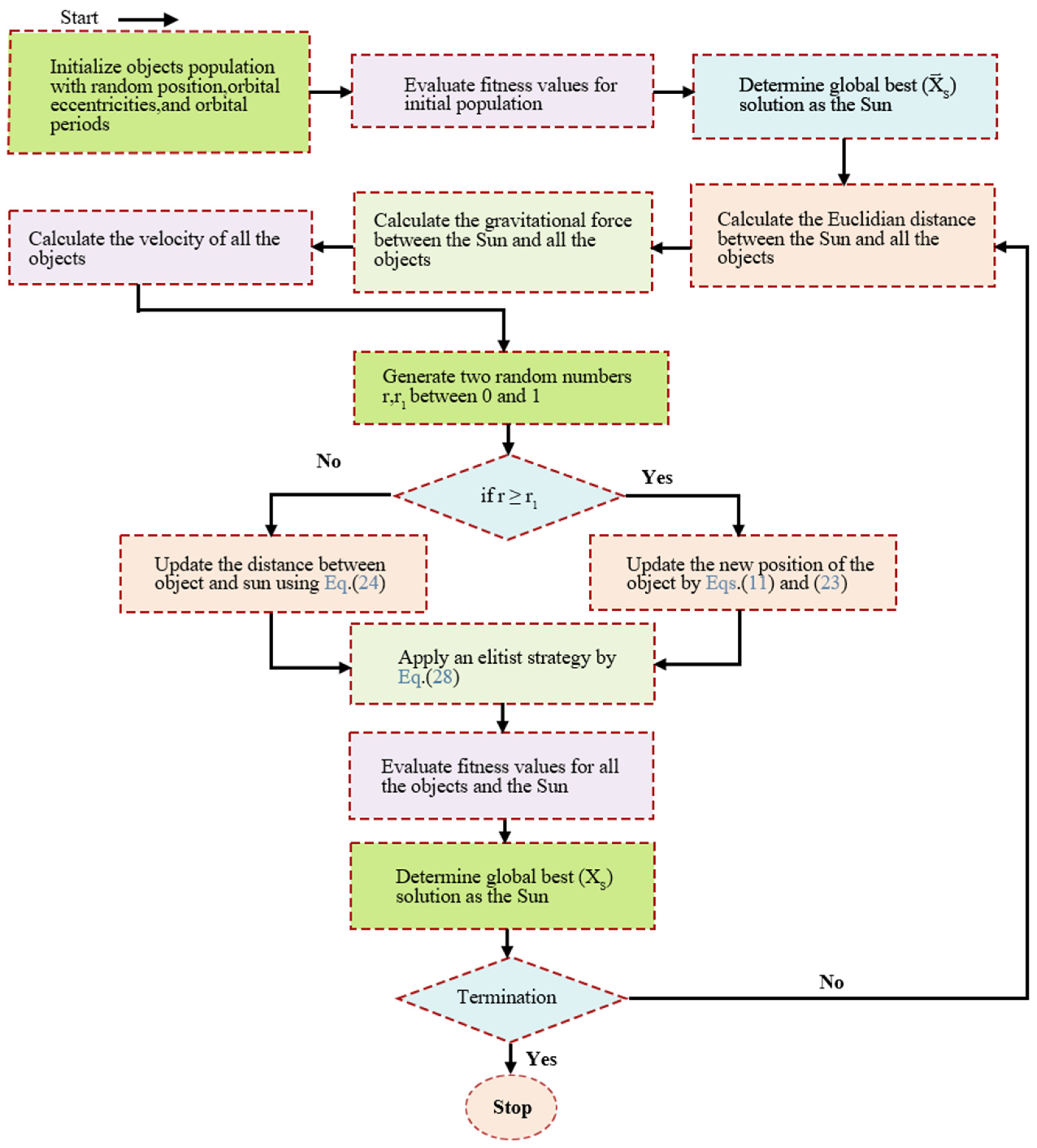
Thus, the specific flow chart of this method is as in Figure 2:

Figure 2. Flow chart KOA optimization algorithm.

Summary of KOA

The Kepler Optimization Algorithm (KOA) is a heuristic optimization method inspired by the motion of planets around the sun, as proposed by Abdel-Basset et al. In the KOA, candidate solutions, represented as planets, orbit an optimal solution, the sun, in elliptical paths, allowing efficient exploration and exploitation of the search space. The process begins with the random distribution of candidate solutions, followed by the selection of orbital periods and eccentricities from normal and uniform distributions. The fitness of each solution is then calculated to evaluate its quality. During iterative optimization, the best solution serves as the sun, guiding the movement of planets. The velocity of each planet changes based on its distance from the sun, simulating gravitational effects to balance exploration and exploitation. The KOA employs mechanisms to escape local optima by randomly adjusting the search direction. An elite strategy ensures the best solutions are retained and refined, making the KOA a robust global optimization algorithm well suited for complex optimization problems and enhancing prediction accuracy in load forecasting models.

2.3. The BiGRU Model

LSTM is developed from RNN, which changes the neurons in the hidden layer of RNN through the gate mechanism and introduces a self-loop mechanism on the basis of it to improve the shortcomings of gradient disappearance. As a variant of LSTM, the GRU neural network has been optimized in structure, reducing the training time while ensuring high-accuracy prediction. Compared to LSTM, GRU is more concise in design and its structure contains only two gates: the reset gate ($r$) and update gate ($z$). The former mainly controls data (or variables?), the input of data, and the composition of previous memory and the latter controls the preservation of the previous memory. The simplified structure of GRU enables it to model sequences for the temporal characteristics of data effectively while maintaining high computational efficiency. The following Formulas (29) and (30) show the governing formulas for GRU units:

$$z_t={\theta }_m(H_z{x}_t+Q_z{l}_{z-1}+a_z)$$

(29)

$$r_t={\theta }_m(H_t{x}_t+Q_r{l}_{t-1}+a_z)$$

(30)

where, in Equations (8) and (9), $H_z$, $H_r$, $Q_z$, $Q_r$, and the corresponding activation functions ${\theta }_g$ as well as the bias $a_z$, $a_r$, update $r_t$, and reset $z_t$ gate are calculated based on the assigned weights. In addition, $x_t$ is the input to the neuron at the time step, $t$ and $h_{t-1}$ is the cell state vector at the time step $t-1$. After this, the reset gate $r_t$ is used to start new memory contents. The Hadamard (element product) is calculated using the formula $Q_z\circ l_{t-1}$. The reset gate $r_t$ is used to determine what information to eliminate from the previous step. After that, the activity function is applied to produce a new cell state vector $\widetilde{g_t}$.

Finally, the current cell state vector $h_t$ is obtained by passing the reservation information to the next cell. To this end, updating the gate $z_t$ involves the Formulas (31) and (32):

$$\widetilde{g_t}={\theta }_{mg}\left[H_g{x}_t+(r_t\circ Q_g{l}_{t-1})+a_g\right]$$

(31)

$$g_t=z\circ l_{t-1}(1+z_t)\circ \widetilde{g_t}$$

(32)

For information retrieval and storage, the GRU neural network adopts a recurrent structure. Still, this structure only considers the previous state of the prediction point, ignoring the future state of the prediction point. However, in actual forecasting, the load information at the previous time is always highly related to the load information at the next time. Therefore, the prediction accuracy cannot be further improved. For deeper time series feature extraction, the BiGRU is introduced here.

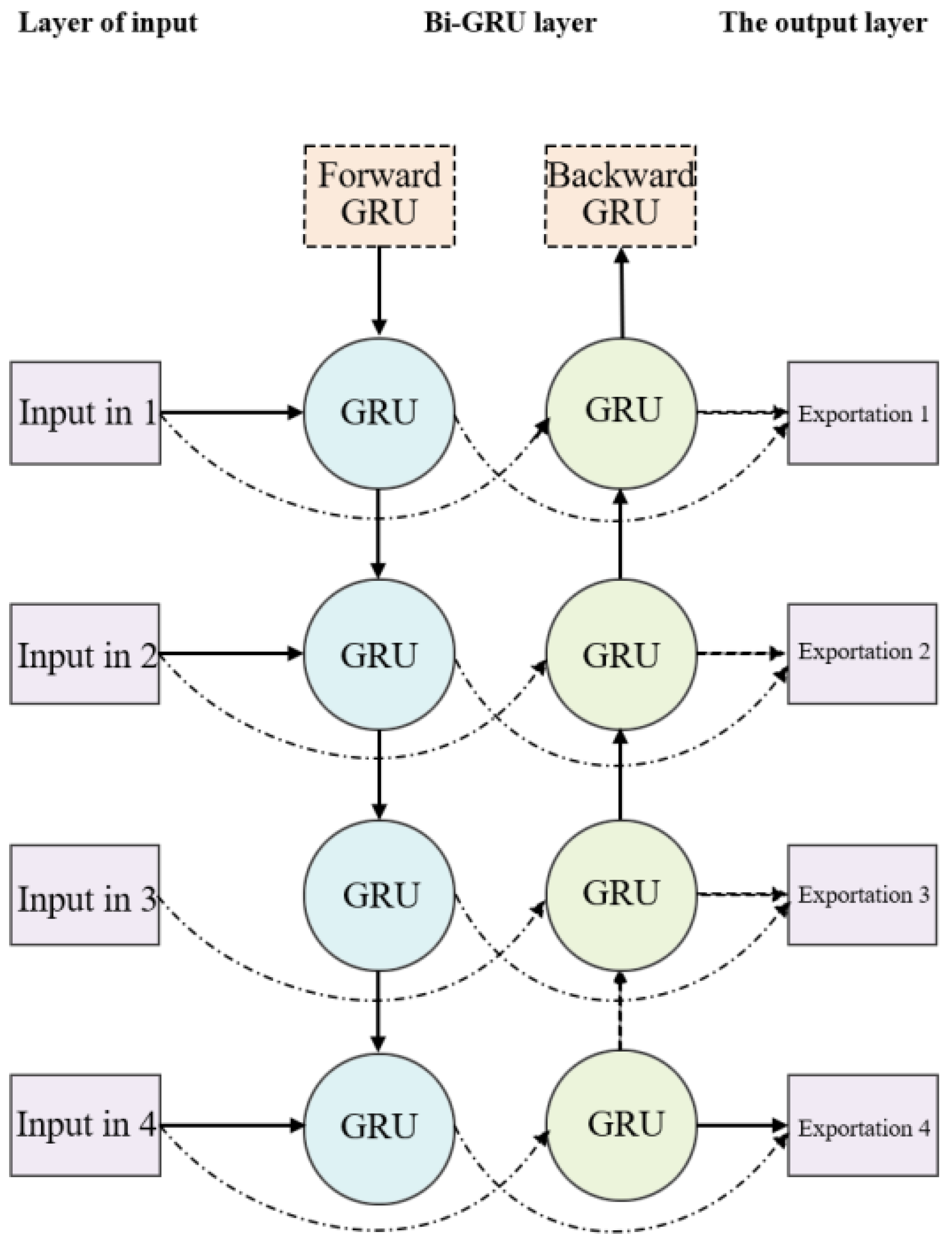
The BiGRU (bidirectional recurrent neural network) consists of a forward GRU layer and an inverse GRU layer, which allows for predicting time series in the opposite direction. In the end, the output will be determined by the state of the forward and inverse layers. Due to the absence of a connection between the forward and inverse layers, BiGRU enables simultaneous consideration of data change patterns compared to one-way GRU, thereby enhancing flexibility, comprehensiveness, and relevance in analysis. This promotes a stronger integration between the model and its processing information while significantly improving prediction accuracy compared to GRU. The structure of BiGRU is shown in Figure 3 and the expression of the network structure is as in Formulas (33)–(35).

$$\overrightarrow{g_t}=GRU(x,\overrightarrow{g_t})$$

(33)

$$\overleftarrow{g_t}=GRU(x,\overleftarrow{g_t})$$

(34)

$$g_t=H_{\overrightarrow{g_t}}\overrightarrow{g_t}+H_{\overleftarrow{g_t}}\overleftarrow{g_t}+a_t$$

(35)

where GRU is the traditional GRU network operation process, $H_{\overrightarrow{g_t}}$ and $\overrightarrow{g_t}$ are the state and weight of the forward hidden layer at time $t$, $H_{\overleftarrow{g_t}}$ and $\overleftarrow{g_t}$ are the state and weight of the backward hidden layer at time $t$ and $a_t$ is the bias of the hidden layer at time $t$.

Figure 3. Diagram of the BiGRU structure.

The specific structure of the BiGRU is shown in Figure 3.

2.4. BiTCN Model

Time convolutional network (TCN) models have gained significant attention and application in the field due to their ability to process time series data in parallel efficiently. Similarly, the study and application of BiLSTM networks have been validated to capture important fluctuation characteristics associated with future time parameters. However, it should be noted that in predicting the current power load, TCN is limited to capturing past parameter fluctuations such as wind speed, temperature, and rate of change. In summary, this paper proposes to optimize the power load forecasting model using the BiTCN algorithm.

The BiTCN model facilitates bidirectional information integration by simultaneously capturing the fluctuation characteristics of parameter changes in both past and future time dimensions. It achieves this by connecting forward TCN modules, backward TCN modules, and a temporal attention module within each BiTCN module. Multiple BiTCN modules are sequentially connected to construct the overall BiTCN model.

The forward TCN model receives past time parameters as inputs from the module, while the backward TCN model takes future time parameters as inputs. Both models share consistent input parameters and employ temporal attention to merge and process the outputs from both modules, resulting in a novel set of output features. Element-wise input fusion significantly enhances the performance of the model.

We are assuming that the input to the module $L$ in the BiTCN model is $X_L$, where $X_L=\left\{X_1,X_2,X_3\dots X_t\right\}$. Firstly, $X_L$ is fed into the forward TCN module to extract historical temporal information from the vibration data and obtain bold time features $\overrightarrow{{\sigma }_t}$. Simultaneously, by applying reverse processing on $X_L$, we accept backward time data $\overleftarrow{X_L}$, where $\overleftarrow{X_L}=\left\{X_t,{ X}_{t-1}, X_{t-2}\dots X_1\right\}$. Then, it serves as input for the back TCN module to extract future temporal information from the vibration data and acquire backward time features $\overleftarrow{{\sigma }_t}$. The formulas for calculating these two types of features are Formulas (36) and (37):

$$\overrightarrow{{\sigma }_t}=\overrightarrow{\mathrm{TCN}}({\mathbf{X}}_L,\delta ,\omega ,d,\tau )$$

(36)

$$\overleftarrow{{\sigma }_t}=\overleftarrow{\mathrm{TCN}}(\overleftarrow{{\mathbf{X}}_L},\delta ,\omega ,d,\tau )$$

(37)

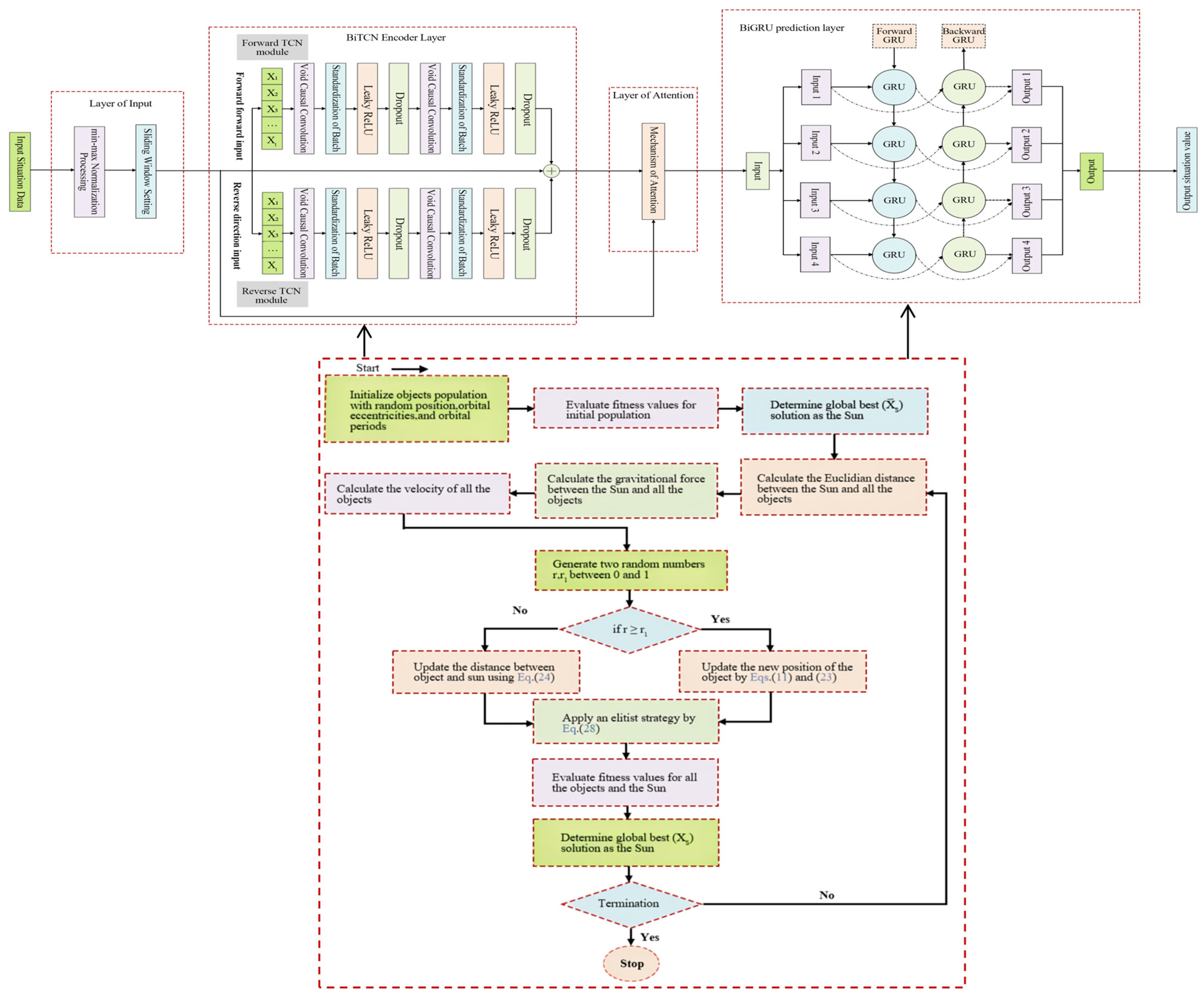
The dimensions of the temporal convolutional kernel for capturing time gaps, the parameter for the leaky ReLU activation function, the dilation rate for atrous convolution, and the parameter for dropout regularization are represented by $\delta$, $\omega$, $d$, and $\tau$, respectively. $\overrightarrow{\mathrm{TCN}}(·)$ denotes feature extraction in the forward TCN module while describing feature extraction in the backward TCN module. The structure of BiTCN is shown in Figure 4.

Figure 4. BiTCN module structure.

2.5. The Attention Mechanism

The attention mechanism is a computational approach that emulates the information processing mechanism of the human brain, thereby enhancing the information processing capability of neural networks. It selectively emphasizes important features by assigning weights to input features and applying weight distribution to retain intermediate results in neural network computations. This facilitates learning with a new model while reducing or disregarding the influence of irrelevant features, thus achieving effective information filtering, improving analysis efficiency, enabling better decision-making by models, and enhancing prediction accuracy. For short-term load forecasting tasks, models often need to process large volumes of load data within limited time frames. The value of the load at a specific moment is more closely related to nearby load values than those further away. Therefore, models should primarily focus on recent load values during prediction. This necessitates leveraging attention mechanisms. The attention mechanism can assign varying weights to each time point’s load value by giving higher weights to values closer in time and lower weights as they become more distant from the current time point. Consequently, models can effectively capture valuable information quickly and improve prediction accuracy. Figure 5 illustrates the structure of an attention mechanism representing an attention distribution vector.

Figure 5. Attention mechanism.

The relevant formulas for this mechanism are Formulas (38)–(40):

$$e_t=v\tanh (W{h}_t+b)$$

(38)

$${\alpha }_1=softmax(e_t)={\displaystyle \frac{\exp (e_t)}{{\displaystyle \sum _{j=1}^m{e}_j}}}$$

(39)

$$y_i={\displaystyle \sum _{j=1}^m{\alpha }_j}{h}_j$$

(40)

The attention-scoring function $e_t$ is in the hidden layer $h_t$, while $v$ and $W$ represent the attention weights. $b$ denotes the bias term and $m$ signifies the dimensionality of input vectors.

2.6. Construction of KOA-BiGRU-BiTCN-Attention Model

To sum up, we can construct the integrated attention mechanism and the BiGRU-BiTCN algorithm optimized by the KOA optimization algorithm as shown in Figure 6:

Figure 6. Structure of KOA-BiGRU-BiTCN-attention model.

The model begins by receiving time series data and conducting preprocessing, which includes data normalization and sliding window processing. The preprocessed time series data is then fed into subsequent network layers for processing. Initially, the data enters the BiTCN module, where each BiTCN module comprises a forward TCN and a backward TCN to capture the forward and backward information of the time series, respectively. Following this, the attention layer takes the output from the BiTCN layer and identifies key information by computing the correlation between elements within the input sequence. The application of the attention mechanism enables the model to focus on the parts of the data that have the greatest impact on the prediction outcomes, thereby enhancing the prediction accuracy. The output of the attention layer is then fed into the BiGRU prediction layer. The BiGRU layer simultaneously handles forward and backward time series information, leveraging its powerful sequence modeling capability to generate more accurate prediction sequences. Finally, the output of the BiGRU prediction layer is processed by the output layer, generating corresponding prediction results based on the specific task requirements. These results can be regression values, classification probabilities, or other forms of output, depending on the model’s training objectives. Throughout the entire training process, the KOA optimization algorithm is employed to fine-tune the model’s hyperparameters, minimizing the loss function on the validation set to improve the model’s generalization ability.

3. Results and Discussion of KOA-BiGRU-BiTCN-Attention Model

To verify the accuracy and generality of the model, this paper selects the wind power dataset from Xinjiang, China, for a verification experiment and a comparison experiment.

3.1. Example of Xinjiang Wind Power Data

This paper utilizes a total of 35,040 load data points from Xinjiang wind power, spanning from 1 January 2019 to 30 December 2019, along with related meteorological and temporal data to construct and verify a power load prediction model. The power load data have a sampling interval of 15 min, resulting in 96 data points sampled each day. For short-term prediction, we selected the first 34,960 data points as the training dataset and the last 100 data points as the validation dataset. For long-term prediction, the first 28,040 data points were chosen as the training dataset and the previous 7000 data points served as the validation dataset.

Data Preprocessing

By checking the data set, it is found that the data set has missing values. The specific missing values are listed in the following Table 1:

Table 1. Number and type of missing values.

Variables with Missing Values	Number of Missing Values
Power load	128
Relative humidity	23
Temperature (°C)	15
Direction of wind	128

Accordingly, we use the KNN algorithm to fill the vacancy value:

First, we randomly delete a part of the data in the complete time series to simulate the missing value through program processing and use the KNN algorithm to perform a filling simulation to test the model performance, as follows in Figure 7 and Table 2:

Figure 7. Imputation of missing values for the KNN model.

Table 2. KNN test performance.

Model	RMSE	MAPE	MAE	R-Squared
KNN	4.97	10.45	379.3	0.97

Then, we apply the model to fill the corresponding vacancy value. Next, we carry out the subsequent screening and variable prediction.

3.2. Selection of Input Variables

After the correlation analysis of different wind speeds, wind direction, and other variables with load data, this paper selects the nine variables with the highest correlation as input variables to train the model and forecast the future load data. The correlation matrix and scatter plots of specific data are shown in Figure 8:

Figure 8. Correlation matrix and scatter plots.

Previous studies have shown that deep learning models are more sensitive to numbers between 0 and 1 [20]. Therefore, prior to inputting the raw load sequence data into the KOA-BiTCN-BiGRU model, we normalized the data. After training, the data were denormalized to obtain the actual load forecast values.

3.3. Selection of Evaluation Indicators

In order to quantitatively evaluate the accuracy of the prediction model, we use three leading evaluation indicators in this paper. These include mean absolute error, which measures the mean fundamental difference between the predicted value and the actual value; the mean fundamental percentage error, which provides the expected error as a percentage of the true value, allowing us to understand the effect of the error in the aggregate; and root-mean-square error, which is the square root of the mean of the squared prediction error and is able to give the magnitude of the prediction error. The specific calculation formula is as follows:

$$RMSE=\sqrt{{\displaystyle \frac{1}{n}}{\displaystyle \sum _{i=1}^n{(p_e(i)-p_a(i))}^2}}$$

(41)

$$MAPE={\displaystyle \frac{1}{N}}{\displaystyle \sum _{i=1}^n\left|\frac{p_e(i)-p_a(i)}{p_e(i)}\right|}\times 100$$

(42)

$$MAE={\displaystyle \frac{1}{n}}{\displaystyle \sum _{i=1}^n\left|p_e(i)-p_a(i)\right|}$$

(43)

where $p_{\mathrm{e}}\left(i\right)$ and $p_{\mathrm{a}}\left(i\right)$ are the predicted value and the measured value, respectively.

3.4. Setting of Model Parameters

Before the experiment starts, we first set the parameters of the relevant model and its optimization algorithm. The relevant parameters of the KOA are as follows Table 3:

Table 3. KOA model parameters.

Parameters	Values
Number of planets to search for	20
Maximum number of function evaluations	5
Range of kernel sizes	[1,5]
Learning rate range	[0.001,0.01]
Range of neuron number	[100,130]

The relevant parameters of the BiGRU-BiTCN-attention optimization algorithm are as follows in Table 4:

Table 4. BiTCN-BiGRU model parameters.

Parameters	Values
Number of planets to search for	20
Maximum number of function evaluations	5
Range of kernel sizes	[1,5]
Learning rate range	[0.001,0.01]
Range of neuron number	[100,130]

3.5. Load Forecasting Experiment Platform and Result Analysis

3.5.1. Experimental Platform

The experiments described in this paper are run on GPU, the graphics card is NVIDIA GeForce GTX 3060, and the experimental environment is MATLAB 2023a edition.

3.5.2. Analysis of Ablation Experiment Results

In this experiment, the prediction results of TCN, GRU, TCN-GRU, and BiTCN-BiGRU prediction methods were taken as the comparison reference, recorded as the experimental control group, and compared with the prediction results of the proposed model to confirm the following two points:

(1)

The feature capture efficiency and prediction accuracy of BiTCN-BiGRU are superior to the basic BiTCN, BiGRU, TCN, and GRU prediction methods.

(2)

The KOA, as a population optimization algorithm, can effectively improve the adjustment efficiency and prediction accuracy of hyperparameters.

Therefore, on the experimental platform, we conducted relevant experiments and obtained the following results in Table 5 and Figure 9:

Table 5. Performance comparison of ablation experiments.

Model	RMSE	MAPE	MAE
GRU	29.71	32.53	31.99
TCN	28.10	31.83	24.30
BiGRU	23.01	29.03	21.68
BiTCN	21.15	28.07	20.33
TCN-GRU	19.71	25.13	19.76
BiTCN-BiGRU	18.05	24.61	18.95
BiTCN-BiGRU-attention	16.44	17.71	14.31
KOA-BiTCN-BiGRU-attention	12.68	10.01	9.93

Figure 9. Visualization of the performance of ablation experiments visualization.

The experimental results show that:

The initial model is a network based on a gated recurrent unit (GRU), which performed worst across all evaluation metrics, including RMSE (31.71%), MAPE (39.53%), and MAE (31.99%). After introducing the temporal convolutional network (TCN), the model’s RMSE, MAPE, and MAE improved by 11.38%, 19.48%, and 24.04%, respectively, indicating TCN’s significant advantage in capturing long-term dependencies of time series. The bidirectional GRU (BiGRU) and bidirectional TCN (BiTCN) structures were further utilized to enhance model performance. Compared to unidirectional TCN, the BiTCN model improved by 8.08%, 3.31%, and 6.23% in RMSE, MAPE, and MAE, respectively. The TCN-GRU model, which combines TCN and GRU, also showed enhanced performance compared to the single BiTCN model, with RMSE improving by 6.81%. Furthermore, the BiTCN-BiGRU-attention model, which combines BiTCN and BiGRU with an attention mechanism, achieved significant performance improvements across all evaluation metrics, with RMSE, MAPE, and MAE improving by 8.92%, 28.04%, and 24.49%, respectively. This indicates that the attention mechanism effectively enhances the model’s ability to recognize essential features in time series, thus improving prediction accuracy. The KOA-BiTCN-BiGRU-attention model, with the introduction of the KOA mechanism, achieved the most significant improvements across all indicators, with RMSE, MAPE, and MAE improving by 22.87%, 43.48%, and 30.61%, respectively.

In summary, our experiments demonstrate that the incorporation of TCN, BiGRU, and the attention mechanism significantly enhances the model’s performance in short-term load forecasting. The KOA mechanism further amplifies these improvements, achieving the highest accuracy among all tested models. These results validate the proposed model’s effectiveness and highlight its potential for practical applications in load forecasting.

At the same time, in order to verify the optimization efficiency of the KOA, this paper selected the BiTCN-BiGRU-attention model optimized by TSA, SMA, GWO, and WOA optimization algorithms for performance comparison. The relevant algorithms are introduced as follows:

The tunicate swarm algorithm (TSA) is a new optimization algorithm proposed by Kaur et al. It is inspired by the swarm behavior of the capsule to survive successfully in the deep sea. The TSA simulates the jet propulsion and swarm behavior of the capsule during navigation and foraging. This algorithm can solve relevant cases with unknown search space [51].

The slime mold algorithm is an intelligent optimization algorithm proposed in 2020, which mainly simulates the foraging behavior and state changes of physarum polycephalum in nature under different food concentrations. Myxomycetes primarily secrete enzymes to digest food. The front end of myxomycetes extends into a fan shape and the back end is surrounded by a network of interconnected veins. Different concentrations of food in the environment affect the flow of cytoplasm in the vein network of myxomycetes, thus forming other states of myxomycetes foraging [30].

The grey wolf optimizer (GWO) is a population intelligent optimization algorithm proposed in 2014 by Mirjalili et al., scholars from Griffith University in Australia. This algorithm is an optimization search method developed inspired by the prey-hunting activities of grey wolves [52].

The whale optimization algorithm (WOA) is a new swarm intelligence optimization algorithm proposed by Mirjalili and Lewis from Griffith University in Australia in 2016. Inspired by the typical air curtain attack behavior of humpback whales in the process of simulating simple prey, the WOA optimized the relevant process [53].

The specific performance is shown in the following Table 6 and Figure 10:

Table 6. Performance comparison of different optimization algorithms.

Model	RMSE	MAPE	MAE
KOA-BiTCN-BiGRU-Attention	12.68	10.01	9.93
TSA-BiTCN-BiGRU-Attention	14.17	11.92	11.27
SMA-BiTCN-BiGRU-Attention	14.60	15.46	12.48
GWO-BiTCN-BiGRU-Attention	14.46	12.86	11.66
WOA-BiTCN-BiGRU-Attention	15.13	13.45	11.96

Figure 10. Visualization of prediction results of different optimization algorithms.

According to the experimental results, the KOA-BiTCN-BiGRU-attention model outperforms other variant models on all evaluation indexes. Specifically, compared to the TSA-BiTCN-BiGRU-attention model, the KOA variant achieved 10.53%, 15.95%, and 11.92% improvement in RMSE, MAPE, and MAE, respectively. Similarly, compared to the SMA-BiTCN-BiGRU-attention model, the KOA variant achieved a 13.15%, 35.32%, and 20.51% improvement on these three metrics, respectively. In addition, compared to the GWO-BiTCN-BiGRU-attention and WOA-BiTCN-BiGRU-attention models, the KOA variant also showed outstanding improvement in RMSE, MAPE, and MAE, reaching 12.32%, 14.47%, 12.21%, 16.19%, 25.58%, and 17.06%, respectively. This proves that the KOA optimization algorithm has obvious advantages over traditional optimization methods.

Then, this paper selects several classical models and sets their relevant parameters consistently with the proposed model for comparative experiments. The models include the decision tree (DT), which builds a tree-like model of decision rules by recursively splitting the dataset into smaller subsets. Each internal node represents a test on an attribute, each branch represents the outcome of the test, and each leaf node represents a prediction result. In time series forecasting, DT predicts a target value at a future point based on feature values from past points in time.

To validate the effectiveness of our proposed model, we compared it against several commonly used time series prediction algorithms, including XGBoost, Gaussian regression, extreme learning machine (ELM), generalized regression neural network (GRNN), generalized additive models regression (GAM), support vector regression (SVR), back propagation neural network (BP), long short-term memory (LSTM), LSTM-CNN, multilayer perceptron (MLP), and MLP-ensemble learning. The specific properties are shown in Table 7 and Figure 11.

Table 7. Classical algorithms predict comparative performance.

Model	RMSE	MAE	MAPE
KOA-BiTCN-BiGRU-attention	12.68	9.93	10.01
XGBoost	20.86	17.14	20.08
Gaussian regression	48.11	38.96	38.01
ELM	48.34	40.29	35.07
GRNN	20.95	16.95	19.63
GAM	30.57	25.53	25.38
SVR	29.40	25.03	27.17
BP	22.09	20.54	20.21
MLP-DT	29.34	24.04	27.58
LSTM	42.32	36.42	40.37
CNN-LSTM	21.55	17.55	19.18

Figure 11. Visualization of comparison of classical algorithm predictions.

In all the above evaluation indicators, the KOA-BiTCN-BiGRU-attention model showed significant performance improvement compared to other models. Compared to the ELM model, the improvement percentage of KOA-BiTCN-BiGRU-attention on RMSE, MAPE, and MAE was 76.80%, 73.46%, and 79.67%, respectively, showing excellent performance for processing very complex time series data. In addition, compared to the classical LSTM model, the improvement in the KOA-BiTCN-BiGRU-attention model in these three indicators reached 71.12%, 74.02%, and 76.01%, respectively, which had different degrees of improvement compared to other models. This further proves the advanced nature and high efficiency of the model proposed in this paper.

The specific improved performance visualization is as follows in Figure 12:

Figure 12. Visualization of performance improvement.

In order to evaluate the computational cost of the proposed model, several experiments were carried out under the same parameter setting and experimental environment and the training time and predicted execution time of the model were recorded. The details are shown in Table 8.

Table 8. Execution time analyses.

Model	Execution Time
KOA-BiTCN-BiGRU-attention	1764 s
TSA-BiTCN-BiGRU-attention	3206 s
SMA-BiTCN-BiGRU-attention	2328 s
GWO-BiTCN-BiGRU-attention	3113 s
WOA-BiTCN-BiGRU-attention	2762 s
XGBoost	1143 s
Gaussian regression	1275 s
ELM	848 s
GRNN	1123 s
GAM	1201 s
SVR	1300 s
LSTM	1132 s
BP	1106 s
MLP-DT	1563 s
CNN-LSTM	1511 s

The KOA-BiTCN-BiGRU-attention model, with an execution time of 1764 s, outperforms other deep learning models optimized with TSA, SMA, GWO, and WOA by offering shorter run times while maintaining high predictive accuracy. Although it has a slightly higher computation time compared to classical models like XGBoost and Gaussian regression, KOA-BiTCN-BiGRU-attention excels in capturing complex time series patterns, especially in tasks involving nonlinearity and long-term dependencies. Its advanced feature extraction and sequence modeling capabilities make it superior in predictive accuracy, showcasing the significant value of deep learning for complex time series forecasting.

In summary, this section verifies the performance of the proposed 24-step multivariable time series short-term load forecasting model. At the same time, we will further study the model in the future to improve its relevant performance and calculation speed.

4. Conclusions

Electricity demand forecasting, a field of long-standing research, has developed various mature prediction models and theories. With the advancement of global “carbon peak and carbon neutrality” goals and the implementation of numerous carbon reduction policies, certain high-energy-consumption and high-emission industries face restrictions or even transformation, while new green industries are emerging rapidly. These changes have led to significant adjustments in China’s industrial structure, rendering traditional statistical methods obsolete. Furthermore, in the context of the construction of new electricity markets, the structure of power systems has become increasingly complex, enabling bidirectional interactions between electricity and information flow and allowing demand-side resources to participate in grid peak shaving and frequency modulation, directly affecting grid loads. Therefore, considering the impacts of “dual carbon” goals, the construction of new power systems is particularly important in mid-to-long-term electricity demand forecasting. Given the differences in principles, advantages, and applicable scenarios of various prediction models, the selection and optimization of models are crucial to ensure adaptability to the complex power system environment under the influence of “dual carbon” goals. Against this backdrop, this study has arrived at the following main conclusions and achievements:

(1)

A novel algorithmic model for short-term load forecasting in a 24-step multivariate time series has been proposed. This model combines KNN data imputation with BiTCN bidirectional temporal convolutional network along with a BiGRU bidirectional gated recurrent unit and attention mechanism. Furthermore, the model’s hyperparameters have been optimized using the Kepler adaptive optimization algorithm (KOA), resulting in enhanced prediction accuracy compared to equivalent time steps.

(2)

An integrated approach has been adopted by combining different models to construct a comprehensive short-term electricity load forecasting model. This holistic framework not only provides valuable insights for production-related decisions but also serves as a reference point for formulating and implementing relevant policies.