Multi-Objective Short-Term Operation of Hydro–Wind–Photovoltaic–Thermal Hybrid System Considering Power Peak Shaving, the Economy and the Environment ^†

Abstract

In recent years, renewable, clean energy options such as hydropower, wind energy and solar energy have been attracting more and more attention as high-quality alternatives to fossil fuels, due to the depletion of fossil fuels and environmental pollution. Multi-energy power systems have replaced traditional thermal power systems. However, the output of solar and wind power is highly variable, random and intermittent, making it difficult to integrate it directly into the grid. In this context, a multi-objective model for the short-term operation of wind–solar–hydro–thermal hybrid systems is developed in this paper. The model considers the stability of the system operation, the operating costs and the impact in terms of environmental pollution. To solve the model, an evolutionary cost value region search algorithm is also proposed. The algorithm is applied to a hydro–thermal hybrid system, a multi-energy hybrid system and a realistic model of the wind–solar–hydro experimental base of the Yalong River Basin in China. The experimental results demonstrate that the proposed algorithm exhibits superior performance in terms of both convergence and diversity when compared to the reference algorithm. The integration of wind and solar energy into the power system can enhance the economic efficiency and mitigate the environment impact from thermal power generation. Furthermore, the inherent unpredictability of wind and solar energy sources introduces operational inconsistencies into the system loads. Conversely, the adaptable operational capacity of hydroelectric power plants enables them to effectively mitigate peak loads, thereby enhancing the stability of the power system. The findings of this research can inform decision-making regarding the economic, ecological and stable operation of hybrid energy systems.

1. Introduction

The accelerated growth of the global economy has resulted in a notable surge in energy consumption [1]. In recent years, the depletion of fossil fuels and the attendant environmental concerns have led to a significant increase in interest in renewable and clean energy sources, including hydro, wind and solar energy sources [2]. It is, thus, evident that the conventional thermal power generation system will undergo a transformation, evolving into a multi-energy complementary power generation system. This system will comprise thermal power, hydropower, wind power, photovoltaic (PV) power and other energy sources, representing a shift from the current single-source approach [3]. As evidenced by the statistical data, the global installed capacity for renewable energy reached 3382 GW by 2021, exhibiting an annual growth rate of approximately 9.4% [4]. The largest share of the renewable energy sources that are currently undergoing intensive development is composed of hydropower, wind and photovoltaics. Specifically, 30.4 GW of new hydroelectric capacity, 73.2 GW of new photovoltaic capacity and 189.2 GW of new wind capacity were recently installed, accounting for 10%, 25% and 65% of renewable energy growth, respectively [4].

However, wind and photovoltaic resources involve strong uncertainty, which limits the development of wind power and photovoltaic power generation [5]. The randomness and volatility of wind and PV options pose a potential risk to the stability of the grid operations when they are integrated into power systems [6]. To overcome this vexing problem, multiple energy sources such as hydropower, thermal power, wind power and PV energy are integrated into the power system to take advantage of the synergistic compensation effect between different energy sources. This can eliminate fluctuations in power generation, improve the stability of the power system’s operation and reduce the cost for power generation. In general, a system in which more than one renewable energy source is operated together is referred to as a hybrid renewable energy system (HRES) [7]. In the past decades, many scholars have studied HRESs, and the current research on HRESs is focused mainly on energy complementary analyses, energy forecasting and the optimal operation. Bhandari et al. [8] collected and analyzed long series of solar radiation, wind speed and ambient temperature data in Nepal and proposed a hybrid system consisting of multi-renewable energy sources of PV, wind and micro-hydropower energy to ensure environmental sustainability. Subsequently, many scholars have verified the feasibility of the grid-connected operation of multiple energy sources by analyzing the characteristics of multiple renewable energy sources, which provides reliable support for the operation of multi-energy complementary systems [9,10,11]. With the vigorous construction and development of wind, photovoltaic and hydropower infrastructure, the prediction and optimal operation of wind, solar and water energy sources have become the focus of research [12,13,14]. A forecasting model for renewable energy has gradually developed from single-site deterministic forecasting [15] to multi-step [16], multi-site [17] and probabilistic forecasting [18], which provides abundant forecasting decision-making information for the optimal operation of multi-energy complementary systems.

The optimal operation of a multi-energy complementary system represents a crucial aspect of HRES research, with the objective of enhancing the operational efficiency and reducing the operational costs. In recent years, numerous scholars have conducted comprehensive research in this field. Qin et al. [19] developed a short-term hydro–thermal scheduling model to reduce the power generation and fuel costs and used a multi-objective optimization method to optimize the model. Hamann et al. [20] presented a simulation method for the real-time operation of a combined hydro–wind system to investigate the ability of a hydro cascade to balance the variability of wind power. Gong et al. [21] devolved a two-period operation model to derive the operating rules for hydro–photovoltaic hybrid systems, considering the diminishing marginal benefit of energy. Li et al. [22] developed a long-term stochastic optimization method for hydro–PV hybrid power plants to maximize the total generation, which is helpful in improving the long-term complementary operation of large-scale hydro–PV hybrid power plants. Qi et al. [23] put forth a methodology for optimally configuring concentrated solar power (CSP) in multi-energy power systems and used a mixed integer linear programming (MILP) formulation to rapidly identify an optimal configuration. Li et al. [24] established a hydro–wind hybrid model to analyze the ability of hydroelectric power to regulate wind power fluctuations and improve financial conditions. Zhang et al. [25] developed a short-term optimal operation model for a wind–solar–hydro hybrid system to minimize the standard deviation of the period power output and maximize the total power generation, and demonstrated the strong adaptive ability of the hydropower plant for the hybrid system. It is evident that the three most prevalent forms of clean energy currently in use are hydropower, wind power and photovoltaic power generation. Among them, hydropower has the characteristics of large regulation volumes, fast load correspondence times and stable generation outputs [26], enabling flexible and complementary optimal scheduling in the HRES, which is an important part of building a clean, low-carbon and multi-energy complementary power system [27].

As demonstrated by the references above, building hybrid hydro–wind–solar systems is an important development trend [28]. However, there is limited research on peak shaving metrics for power systems, with most objective functions focusing on economic metrics, with the ultimate goal of cost reductions [29]. Secondly, although renewable energy sources such as wind, photovoltaic and hydropower sources are being vigorously developed, thermal power is still an indispensable part of the power system, and most existing studies on HRES only consider renewable energy sources and do not consider the grid connection for conventional thermal power [30].

Therefore, the model proposed in this study considers both renewable energy sources such as wind, solar and hydro and conventional thermal power generation in the power system first. Then, a multi-objective, short-term operation model for a hydro–wind–PV–thermal hybrid system is proposed, taking into account the peak shaving, operating costs and environmental impact of the power system. Next, a cost value region search evolutionary algorithm is proposed to solve the multi-objective problem. Meanwhile, the hidden Markov regression is applied to give the probability distribution of the predicted power output to analyze the impact of energy uncertainty on the power system. In conclusion, the main contributions of this paper are as follows:

• A multi-objective, short-term operation model for the hydro–wind–PV–thermal hybrid system (MOHS) considering the peak shaving, operating costs and environmental impact is established.
• The hidden Markov regression method (HMR) and kernelized k-medoids clustering algorithm are applied to analyze the impact of energy uncertainty.
• A new cost value region search evolutionary algorithm (CVRSEA) is proposed to solve the MOHS problem and to demonstrated the flexible operation capability of hydroelectric power plants.

2. Methodology

Most of the existing researchers and scientists consider economic indicators in the optimization of hybrid power systems, with the ultimate goal of cost reductions [31]. However, with the rapid development of wind power and photoelectric energy, power system managers are more concerned with how to dispatch multiple energy loads to ensure the stability of the power system. Therefore, this section proposes a MOHS while considering power peak shaving, the economy and the environment. The power output calculation formulations, objective functions and constraints are described in detail.

2.1. Power Output Calculation

The following formulation represents the potential for hydroelectric power:

$$P_{i,t}^h={\eta }_i{H}_{i,t}{Q}_{i,t}\Delta t$$

(1)

where $P_{i,t}^h$ is the power generation of the i-th hydropower station in period t; η_i is the hydroelectricity coefficient of the i-th reservoir; H_i,t is the water head of the i-th reservoir at period t; Q_i,t is the discharge flow of the i-th reservoir in period t; Δt is the time interval. In addition, the hydroelectric power generation formula needs to take into account the characteristic curve of the hydroelectric unit, which should not exceed the expected output of the power generation at different water heads.

Wind power is a function of the air density, swept area, wind power coefficient and wind speed as follows:

$$P_{i,t}^w={\displaystyle \frac{1}{2}}{\rho }_i{a}_i^w{c}_i^w{v_{i,t}}^3$$

(2)

where $P_{i,t}^w$ is the power generation of the i-th wind farm in period t; ρ_i is the air density of the i-th wind farm; $a_i^w$ is the area swept by the turbine blades at the i-th wind farm; $c_i^w$ is the wind power coefficient of the i-th wind farm; v_i,t is the wind speed of the i-th wind farm in period t. In order to ensure the safe operation of the fan, it is recommended that the wind speed within the specified interval [v_min, v_max] be employed for power generation purposes.

The amount of solar power generated is dependent on two key factors—the intensity of solar radiation and the surface area of the solar power generator:

$$P_{i,t}^s={\eta }_i{a}_i^s{g}_{i,t}$$

(3)

where $P_{i,t}^s$ is the power generation of the i-th solar power plant in period t; η_i is the efficiency of the i-th solar power plant; $a_i^s$ is the solar power generator area of the i-th solar power plant; g_i,t is the solar radiation intensity of the i-th solar power plant in period t. Due to the inherent limitations of the solar panel capacity, it is necessary to regulate the solar power output in interval [$P_{m,\min }^s$, $P_{m,\max }^s$] to ensure an optimal and reliable supply.

2.2. Multi-Objective Operation Model for a Hybrid System

2.2.1. Power Peak Shaving Objective

In the MOHS, the wind power and solar power contain potential uncertainties. To maintain the stability of the electric power system, managers could use the advantages of flexible dispatching for hydropower stations to cut down on peak loads and to smooth the remaining loads for thermal energy. Previous studies have assessed the stability of power systems through the mean square deviation of the remaining loads as follows:

$$\begin{array}{l}\mathrm{MSD}={\displaystyle \frac{1}{T}}{\displaystyle \sum _{t=1}^T{\left(P_t^r-\overline{P}\right)}^2}\\ P_t^r=P_t^d-{\displaystyle \sum _{i=1}^{N_h}{P}_{i,t}^h}+{\displaystyle \sum _{i=1}^{N_w}{P}_{i,t}^w}+{\displaystyle \sum _{i=1}^{N_s}{P}_{i,t}^s}\\ \overline{P}={\displaystyle \frac{1}{T}}{\displaystyle \sum _{t=1}^T{P}_t^r}\end{array}$$

(4)

where $P_t^d$ is the load demand in period t; $P_t^r$ represents the remaining loads in period t; $\overline{P}$ is the average of the remaining loads; N_h is the number of reservoirs; N_w is the number of wind farms; N_s is the number of solar power plants.

In this paper, to eliminate the influence of the magnitude of the remaining load on the mean square deviation, we use a load variation coefficient CV as the optimization objective to demonstrate the level of fluctuation and dispersion of the load, as follows:

$$\min F_1={\displaystyle \frac{\sqrt{MSD}}{\overline{P}}}$$

(5)

2.2.2. Economy Objective

In order to maintain the stability of the electric power system, the managers must strive to minimize the cost of the power system while considering the peak shaving objective of minimizing the deviation of the remaining loads. The fuel cost function of each thermal unit, taking into account valve-point loading effects, is represented by a sum of a quadratic and a sinusoidal function. The total fuel cost of the hybrid systems can be expressed as follows:

$$\min F_2={\displaystyle \sum _{t=1}^T{\displaystyle \sum _{i=1}^{N_T}[{\alpha }_i+{\beta }_i\cdot P_{i,t}^T+{\gamma }_i\cdot {(P_{i,t}^T)}^2}}+\left|{\delta }_i\cdot \sin ({\sigma }_i\cdot (P_{i,\min }^T-P_{i,t}^T))\right|]$$

(6)

where N_T is the number of thermal generators; T is the length of the operation; α_i, β_i, γ_i, δ_i and σ_i are the cost coefficients of the i-th thermal generator; $P_{i,t}^T$ is the power generation of the i-th thermal generator in period t; $P_{i,\min }^T$ is the lower generation limit of the i-th thermal generator.

2.2.3. Emission Objective

Thermal power plants are a significant source of atmospheric pollution, emitting high concentrations of sulfur dioxide (SO₂) and nitrogen oxides (NOx) during the generation of electricity. These pollutants have a detrimental impact on the quality of the surrounding environment. In this study, NOx emissions are employed as the primary indicator to assess the extent of environmental contamination. The objective of the emission can be expressed as follows:

$$\min F_3=\min {\displaystyle \sum _{t=1}^T{\displaystyle \sum _{i=1}^{N_T}[a_i+b_i\cdot P_{i,t}^T+c_i\cdot {(P_{i,t}^T)}^2}}+d_i\cdot \exp (e_i\cdot P_{i,t}^T)]$$

(7)

where a_i, b_i, c_i, d_i and e_i are the emission coefficients of the i-th thermal generator.

2.2.4. Constraints

The constraints of the MOHS are described below.

(1)

In order to ensure the stability of the system, it is essential that the total power generated by hydroelectric stations, thermal generators, wind farms and solar power plants is equal to the system load demand for each time interval:

$$P_t^d={\displaystyle \sum _{i=1}^{N_T}{P}_{i,t}^T}+{\displaystyle \sum _{j=1}^{N_h}{P}_{j,t}^h}+{\displaystyle \sum _{k=1}^{Nw}{P}_{k,t}^w}+{\displaystyle \sum _{m=1}^{N_s}{P}_{m,t}^s}$$

(8)

where $P_t^d$ is the load demand of the wind–solar–hydro–thermal hybrid system during time t; N_h is the number of reservoirs; N_w is the number of wind farms; N_s is the number of solar power plants.

(2)

Power generation limits: The power generation capacity of hydropower stations, thermal generators, wind farms and solar power plants is subject to the maximum and minimum constraints of the generator:

$$P_{i,\min }^T\le P_{i,t}^T\le P_{i,\max }^T$$

(9)

$$P_{j,\min }^h\le P_{j,t}^h\le P_{j,\max }^h$$

(10)

$$P_{k,\min }^w\le P_{k,t}^w\le P_{k,\max }^w$$

(11)

$$P_{m,\min }^s\le P_{m,t}^s\le P_{m,\max }^s$$

(12)

where $P_{i,\min }^T$ and $P_{i,\max }^T$ are the lower and upper generation limits of the i-th thermal generator, respectively; $P_{j,\min }^h$ and $P_{j,\max }^h$ are the lower and upper generation limits of the j-th reservoir, respectively; $P_{k,\min }^w$ and $P_{k,\max }^w$ are the lower and upper generation limits of the k-th wind farm, respectively; $P_{m,\min }^s$ and $P_{m,\max }^s$ are the lower and upper generation limits of the m-th solar power plant, respectively.

(3)

Water balance equation:

$$V_{i,t}=V_{i,t-1}+\left(I_{i,t}-Q_{i,t}\right)\Delta t$$

(13)

where I_i,t is the inflow of the i-th reservoir during time t; Q_i,t is the outflow of the i-th reservoir during time t; Δt is the time interval; V_i,t is the storage volume of i-th reservoir at time t.

(4)

Continuity equation for the cascade reservoirs:

$$I_{i,t}=q_{i,t}+{\displaystyle \sum _{k=1}^{N_{ui}}{Q}_{k,t-T_{ki}}}$$

(14)

where q_i,t is the interval runoff during time t; N_ui is the number of upstream reservoirs above the i-th reservoir; T_ki is the time delay from reservoir k to j.

(5)

Reservoir discharge constraints:

$$Q_{i,\min }\le Q_{i,t}\le Q_{i,\max }$$

(15)

where $Q_{i,\min }$ and $Q_{i,\max }$ are the lower and upper discharge limits of the i-th reservoir, respectively.

(6)

Reservoir storage volumes constraints:

$$V_{i,\min }\le V_{i,t}\le V_{i,\max }$$

(16)

where $V_{i,\min }$ and $V_{i,\max }$ are the lower and upper limits of the volume of i-th reservoir, respectively.

(7)

The initial and terminal reservoir storage volume limits are as follows:

$$V_{i,0}=V_i^{start},V_{i,T+1}=V_i^{end}$$

(17)

where $V_i^{start}$ and $V_i^{end}$ are initial and terminal storage volume of i-th reservoir, respectively.

2.3. Representation of Uncertainty

The existing complementary power generation systems are generally equipped with mature commercial forecasting products, which can provide short-term deterministic forecasts for wind and solar power outputs. Most of these products use forecast models based on physical mechanisms. However, there are prediction errors and potential uncertainties in the prediction of wind and solar power outputs, which affect the power supply stability of the power system. Therefore, it is necessary to represent the uncertainty in wind and solar power output predictions and provide sampling boundaries for the stochastic simulation.

2.3.1. Uncertainty Analysis

To quantify the prediction uncertainty associated with the prediction of wind and solar power outputs, the HMR [12] is employed to provide a probability distribution for the predicted power output. In the HMR, the observation model is assumed to be a joint Gaussian distribution, whereby the joint data x can be divided into two subvectors, x = [x¹; x²], where x¹ denotes the forecasting result of the mature commercial forecasting products and x² denotes the observed power output. Finally, the uncertainty of the power output can be quantified as follows:

$$\begin{array}{l}p\left(x_t^2\left|x_t^1\right.\right)={\displaystyle \frac{p\left(x_t^1,x_t^2\right)}{p\left(x_t^1\right)}}\\ \hspace{0.33em}\hspace{0.33em}\hspace{0.33em}\hspace{0.33em}\hspace{0.33em}\hspace{0.33em}\hspace{0.33em}\hspace{0.33em}={\displaystyle \frac{{\displaystyle \sum _{k=1}^K\left[\left({\displaystyle \sum _{i=1}^K{h}_{t-1}\left(i\right)A_{ik}}\right)N\left(x_t^1\left|{\mathit{\mu }}_1^k,{\sum }_{11}^k\right.\right)N\left(x_t^2\left|{\mathit{\mu }}_{2\left|1\right.}^k,{\sum }_{2\left|1\right.}^k\right.\right)\right]}}{{\displaystyle \sum _{j=1}^K\left[\left({\displaystyle \sum _{i=1}^K{h}_{t-1}\left(i\right)A_{ij}}\right)N\left(x_t^1\left|{\mathit{\mu }}_1^j,{\sum }_{11}^j\right.\right)\right]}}}\\ \hspace{0.33em}\hspace{0.33em}\hspace{0.33em}\hspace{0.33em}\hspace{0.33em}\hspace{0.33em}\hspace{0.33em}\hspace{0.33em}\hspace{0.33em}={\displaystyle \sum _{k=1}^K{h}_t\left(k\right)}N\left(x_t^2\left|{\mathit{\mu }}_{2\left|1\right.}^k,{\sum }_{2\left|1\right.}^k\right.\right)\end{array}$$

(18)

$$h_t\left(k\right)={\displaystyle \frac{\left({\displaystyle \sum _{i=1}^K{h}_{t-1}\left(i\right)A_{ik}}\right)N\left(x_t^1\left|{\mathit{\mu }}_1^k,{\sum }_{11}^k\right.\right)}{{\displaystyle \sum _{j=1}^K\left[\left({\displaystyle \sum _{i=1}^K{h}_{t-1}\left(i\right)A_{ij}}\right)N\left(x_t^1\left|{\mathit{\mu }}_1^j,{\sum }_{11}^j\right.\right)\right]}}}$$

(19)

where K is the number of states; π_k is the initial probability of state k; μ_k and Σ_k are the mean vector and covariance matrix of the k-th joint Gaussian distribution, respectively; h_t (k) represents the HMM forward variable.

2.3.2. Simulation Scenarios

After obtaining the output probability density function given in the uncertainty analysis, we can use the Monte Carlo simulation method to randomly sample the forecasted wind power and photovoltaic energy. However, the use of too many scenarios will reduce the computational efficiency of the MOHS. The scenario reduction process has the potential to enhance the computation speed of a given operation without compromising the integrity of the information contained within the scenarios themselves. In order to reduce the number of scenarios in an effective manner, a kernelized k-medoids clustering algorithm is employed for clustering scenarios that are deemed to be similar. The process is as listed below.

Step 1: Randomly select K centroids m_1:K from the generated scenarios {1, …, N}.

Step 2: Calculate the kernel function for each scenario in comparison to the cluster centroids d (i, m_k), i = 1, …, N:

$$d\left(i,m_k\right)\triangleq k\left(x_i,x_{m_k}\right)=\exp \left(-{\displaystyle \frac{{‖x_i-x_{m_k}‖}^2}{2{\sigma }^2}}\right)$$

(20)

Step 3: Identify the nearest cluster centroids and assign a scenario to each of them:

$$z_i=\underset{m_k}{\mathrm{argmax}} d\left(i,m_k\right)\hspace{0.33em}$$

(21)

Step 4: Update the cluster centroids:

$$m_k=\underset{i:z_i=k}{\mathrm{argmax}}{\displaystyle \sum _{i^{\prime }:{z^{\prime }}_i=k}d\left(i,i^{\prime }\right)}$$

(22)

Step 5: Evaluate the convergence. If convergence is achieved, the process should be continued; otherwise, the procedure should be repeated from step 2

Step 6: After the clustering, we can get K clusters form the generated scenarios, which can be regarded as representative scenarios.

3. Cost Value Region Search Evolutionary Algorithm

The power generation output of the thermal generators and the discharge flow of the hydropower stations are defined as the optimization variables of the hybrid system multi-objective operation model. This optimization model involves a multi-stage decision-making, multi-constraint, multi-objective, nonlinear optimization problem, which is difficult to solve efficiently using conventional optimization algorithms [32]. Therefore, this paper proposes a cost value region search evolutionary algorithm (CVRSEA) to solve this problem.

3.1. Region Search Strategy

The main technology used for the region search strategy includes regional division, regional identification, regional mating selection and regional update strategies.

3.1.1. Regional Division and Identification

The region search strategy uses a predefined set of regions to balance the population diversity and convergence. First, we use Das and Dennis’s [33] systematic approach to predefine a set of evenly spread weight vectors (λ¹, λ²,…, λ^N) on a hyperplane in the objective space. Then, the objective space is divided into N regions according to the Euclidean distance of the point coordinate and the weight vector, as shown in Figure 1.

The cosine similarity function is used to identify the corresponding region of each individual. The cosine similarity between a solution xⁱ and a weight vector λ^k is defined as follows:

$$\cos 〈{\mathit{x}}^i,{\mathit{\lambda }}^k〉={\displaystyle \frac{{\left({\mathit{f}}^i\right)}^T{\mathit{\lambda }}^k}{‖{\mathit{f}}^i‖\cdot ‖{\mathit{\lambda }}^k‖}}$$

(23)

where ${\mathit{\lambda }}^k={\left({\lambda }_{k,1},\dots ,{\lambda }_{k,M}\right)}^T$ is the k-th weight vector, whereby $\forall m=1,\dots ,M$, ${\lambda }_{k,m}\ge 0$ and ${\displaystyle {\sum }_{m=1}^M{\lambda }_{k,m}}=1$; M is the number of objectives; ${\mathit{f}}^i$ denotes the objective value vector of xⁱ; ‖ ‖ denotes the Euclidean distance.

Based on the cosine similarity values between solution xⁱ and all weight vectors, the region of solution xⁱ can be found as follows:

$$r^i=\underset{k}{\mathrm{argmax}}\hspace{0.33em}\cos 〈{\mathit{x}}^i,{\mathit{\lambda }}^k〉\hspace{0.33em}k=1,\dots ,N$$

(24)

where rⁱ is the region index of solution xⁱ.

3.1.2. Regional Mating Selection and Regional Update

Individual reproduction and population updates are the main processes that affect the convergence and diversity of the algorithm. For the CVRSEA, a regional mating selection strategy and regional update strategy are proposed to balance the convergence and diversity of the algorithm.

For the regional mating selection strategy, we first use a cosine similarity function to define the neighbor regions NR_k for each region k. When generate a new offspring in each region k, and the parent solutions for the recombination operator are selected from the neighbor regions NR_k. For example, the differential evolution operator needs three parent solutions to generate the offspring; three parent solutions indexes s₁, s₂ and s₃ are selected from the neighbor regions NR_k, where s₁, s₂ and s₃ satisfy s₁ ≠ s₂ ≠ s₃ ≠ k. This strategy can greatly improve the convergence of the algorithm but it is easy for convergence to occur locally in the early stage of the algorithm’s evolution, resulting in a lack of population diversity.

After an offspring solution x^c is generated by the reproduction procedure, we can compare the offspring solution x^c with the old parent solution x^k in region k. With the regional update strategy, we first identify the region r^c that the offspring solution x^c belongs to. Then, we compare the region of the parent solution and the offspring solution; if solution x^c belongs to region k or the cosine similarity value of the offspring solution cos < x^c, λ^k> is greater than or equal to cos < x^k, λ^k>, the offspring solution x^c can replace the parent solution x^k. This strategy avoids the local convergence of the algorithm in the early stage and does not lose the convergence of the algorithm in the later stage of evolution.

3.2. Cost Value Based Archive Set

The main idea is that the region search strategy uses a predefined set of regions to guide the evolution direction of the population, so that the algorithm converges quickly in a uniform hyperplane. However, many real-world multi-objective problems, especially those with multiple constraints such as the proposed multi-objective operation model of the hybrid system, have discontinuous Pareto fronts [34]. Therefore, an archive set based on the cost value [35] is applied in the CVRSEA.

During the reproduction and population update process, all generated offspring solutions are added into the archive set. When the size of the archive set is larger than the predefined size N_arc, the archive set will be trimmed based on the cost value and cosine similarity value. The cost value of each individual in the archive set can be calculated as follows:

$$c{v}_i=\underset{j\ne i}{\min }{c}_{ij},\hspace{0.33em}\hspace{0.33em}\hspace{0.33em}j=1,\dots ,N_{all}$$

(25)

$$c_{ij}=\underset{m}{\max }{f}_m^j/f_m^i,\hspace{0.33em}\hspace{0.33em}\hspace{0.33em}m=1,\dots ,M$$

(26)

where cv_i is the cost value of individual xⁱ; N_all is the size of the archive set; cij is the mutual evaluation value between individuals xⁱ and x^j; $f_m^i$ is the m-th objective value of individual xⁱ. If the cost value cv_i is greater than 1, then xⁱ is a non-dominated solution in the archive set; otherwise, xⁱ is a dominated solution.

In the archive set trimming process, if the number of individuals with cv > 1 is smaller than N_arc, the N_arc individuals with the greatest cost value are selected. If the number of individuals with cv > 1 is larger than N_arc, all individuals with cv ≤ 1 are removed and then the cosine similarity matrix among the remaining individuals is calculated as follows:

$$\cos 〈{\mathit{x}}^i,{\mathit{x}}^j〉={\displaystyle \frac{{\left({\mathit{f}}^i\right)}^T{\mathit{f}}^j}{‖{\mathit{f}}^i‖\cdot ‖{\mathit{f}}^j‖}}$$

(27)

Finally, the two individuals with the largest cosine similarity are found, and the individual with the smaller cost value. The above procedure will be executed for (N_{cv > 1} − N_arc) times. After this, the N_arc individuals with the better convergence and distribution in archive set have been determined.

3.3. Framework for the Proposed Algorithm

The framework for the proposed CVRSEA is presented in Algorithm 1. In the initialization procedure, a set of N regions is generated. Subsequently, the neighbor regions index set NR is initialized according to the cosine similarity value of the regions. In the main loop, for each predefined region, a new offspring is generated in accordance with the reproduction procedure. Following reproduction, the parent solution is replaced by the offspring in accordance with the regional update strategy and the offspring is added to the archive set. After updating all populations, the archive set is trimmed based on the cost value and cosine similarity value.

Algorithm 1: Framework for the CVRSEA

1   (λ1, λ2,…, λN) = Initialization() 2  NR = InitializeNeighborRegions() 3  P = InitializePopulation() 4  while termination criteria is not satisfied do 5      for each region k = 1, 2, … , N do 6          $Set\hspace{0.33em}MP=\left\{\begin{array}{l}N{R}_k\hspace{0.33em}\hspace{0.33em}\hspace{0.33em}\hspace{0.33em}\hspace{0.33em}\hspace{0.33em}\hspace{0.33em}\hspace{0.33em}\hspace{0.33em}\hspace{0.33em}\hspace{0.33em}\hspace{0.33em}\hspace{0.33em}random<0.9\\ Archive set\hspace{0.33em}\hspace{0.33em}\hspace{0.33em}\mathrm{otherwise}\end{array}\right.$ // determine the mating pool 7          xc = Reproduction(MP) // xc is an offspring 8  P = UpdtaePopulation(MP, xc) 9          ArcSet = ArcSet $\cup$ {xc}; 10      end for 11      ArcSet = UpdtaeArcSet(ArcSet) 12 end while

3.4. Constraint Handling Method

The multi-objective operation model of a hybrid system comprises a substantial number of inequality and equality constraints, which presents a challenge for the algorithmic approach in producing solutions that adhere to all constraints throughout the evolutionary process. The inequality constraints are relatively simple to deal with, for we can adjust them to be equal to the boundaries when they are out of their boundaries during the reproduction process. However, equality constraints are more difficult to handle when compared with inequality constraints, such as power balance constraints (see Equation (7)) and final reservoir storage volume constraints (see Equation (16)).

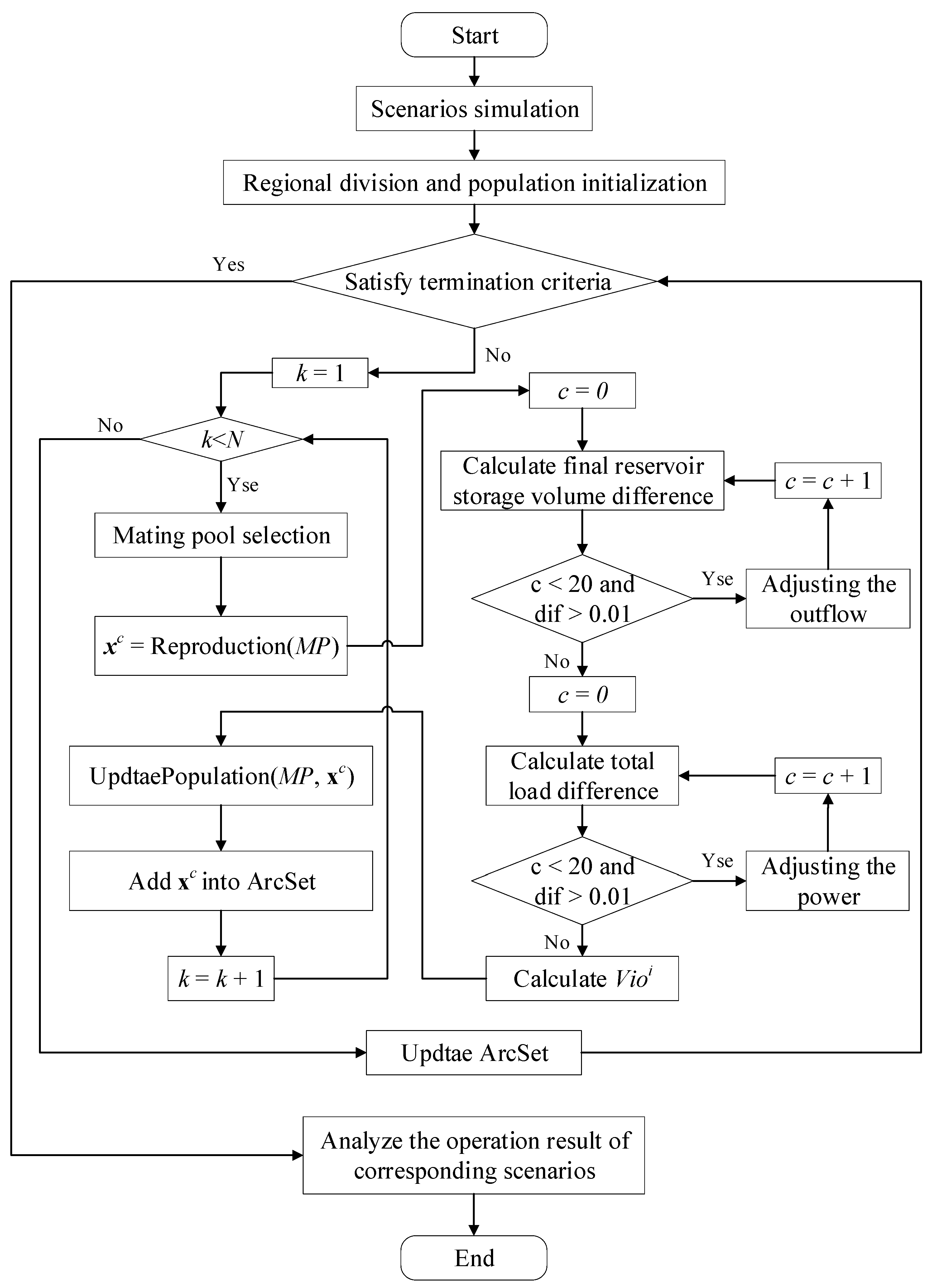
The power balance and final reservoir storage volume constraints are affected by the power generation and the outflow of the reservoir during the whole dispatch period. Therefore, in this paper, we calculate the total load and final reservoir storage volume difference and then iteratively modify the outflow of the reservoirs and thermal power generated for each period to meet the constraints as much as possible. The adjustment of the outflow of the reservoir will change the output of the hydropower plant, thus affecting the power balance constraint. Therefore, the final storage volume for each reservoir is handled firstly by adjusting the outflow of the hydropower plant, and then the power balance constraint is handled by adjusting the output of the thermal power unit (without changing the outflow and output of the hydropower plant, thus not affecting the final storage volume of each reservoir). The individual repaired according to the above method is generally a feasible individual, although because only a limited number of adjustments are made, the individual may still violate the constraint. The violation value Vioⁱ of individual xⁱ is calculated as follows:

$$Vi{o}^i={\displaystyle {\sum }_{j=1}^{N_h}|V_{j,T+1}-}{V}_j^{end}|+{\displaystyle {\sum }_{t=1}^T|\Delta P_t|}$$

(28)

$$\Delta P_t=P_t^d-\left({\displaystyle \sum _{i=1}^{N_T}{P}_{i,t}^T}+{\displaystyle \sum _{j=1}^{N_h}{P}_{j,t}^h}+{\displaystyle \sum _{k=1}^{Nw}{P}_{k,t}^w}+{\displaystyle \sum _{m=1}^{N_s}{P}_{m,t}^s}\right)$$

(29)

For the constraint problem, the population update procedure for the CVRSEA is modified as follows: (1) if the violation value Vioⁱ is less than the violation value Vio^j, individual i is better than individual j; (2) if the violation value Vioⁱ is equal to the violation value Vio^j, we compare the two individuals according to the original method, using the dominance relationship, aggregation function and cost value. The flowchart for the implementation of the CVRSEA to solve the multi-objective operation model of the hybrid system is shown in Figure 2.

4. Results

4.1. Simulation Data

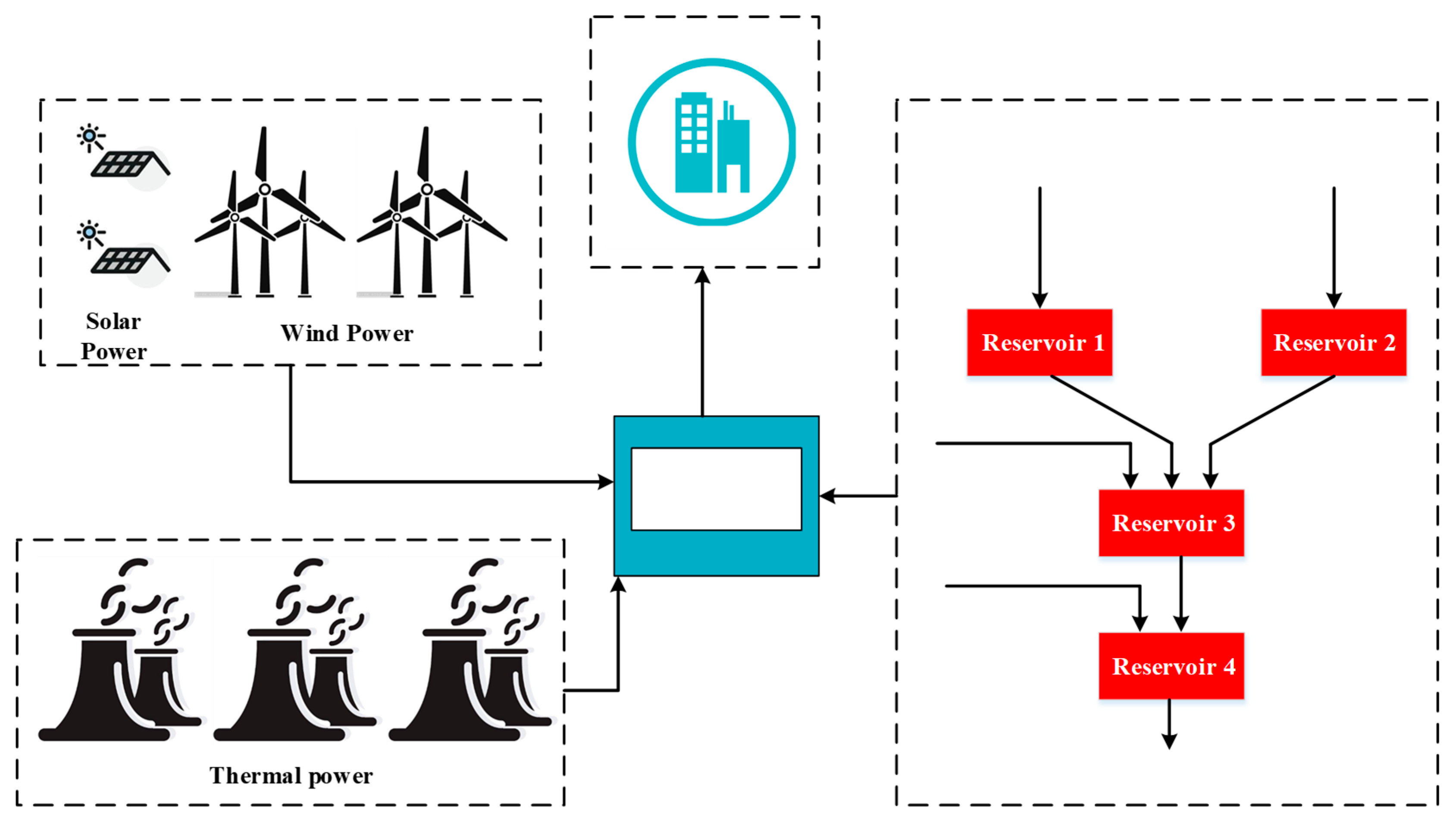
In this section, a case study is conducted to validate the proposed MOHS. The hybrid system consists of a multi-chain cascade of four hydro plants, three thermal units, two wind power plants and two photovoltaic plants, and the system diagram is shown in Figure 3. The operational period is 24 h in duration, with a time step of one hour.

Table 1. The load demand and inflow volume.

Time	Pd	R1	R2	R3	R4
1	750	10	8	8.1	2.8
2	780	9	8	8.2	2.4
3	700	8	9	4	1.6
4	650	7	9	2	0
5	670	6	8	3	0
6	800	7	7	4	0
7	950	8	6	3	0
8	1010	9	7	2	0
9	1090	10	8	1	0
10	1080	11	9	1	0
11	1100	12	9	1	0
12	1150	10	8	2	0
13	1110	11	8	4	0
14	1030	12	9	3	0
15	1010	11	9	3	0
16	1060	10	8	2	0
17	1050	9	7	2	0
18	1120	8	6	2	0
19	1070	7	7	1	0
20	1050	6	8	1	0
21	910	7	9	2	0
22	860	8	9	2	0
23	850	9	8	1	0
24	800	10	8	0	0

presents the load demand and the inflow of each reservoir. The coefficients for hydropower generation and thermal generation, reservoir limits and generation limits are set at the same values as the reference [19].

4.2. Results without Wind–Solar Energy

In order to ascertain the efficacy of the CVRSEA, we initially implement it in a system that does not consider solar or wind power. In this case, we consider only the economic and emission objectives and compare the results with the MODE-ACM algorithm [19] under the same conditions. The parameters of the CVRSEA are set as follows: population size = 100, neighbourhood size = 20, archive set size = 30, mutation probability = 1/100, mutation distribution index = 20, number of generations = 2000.

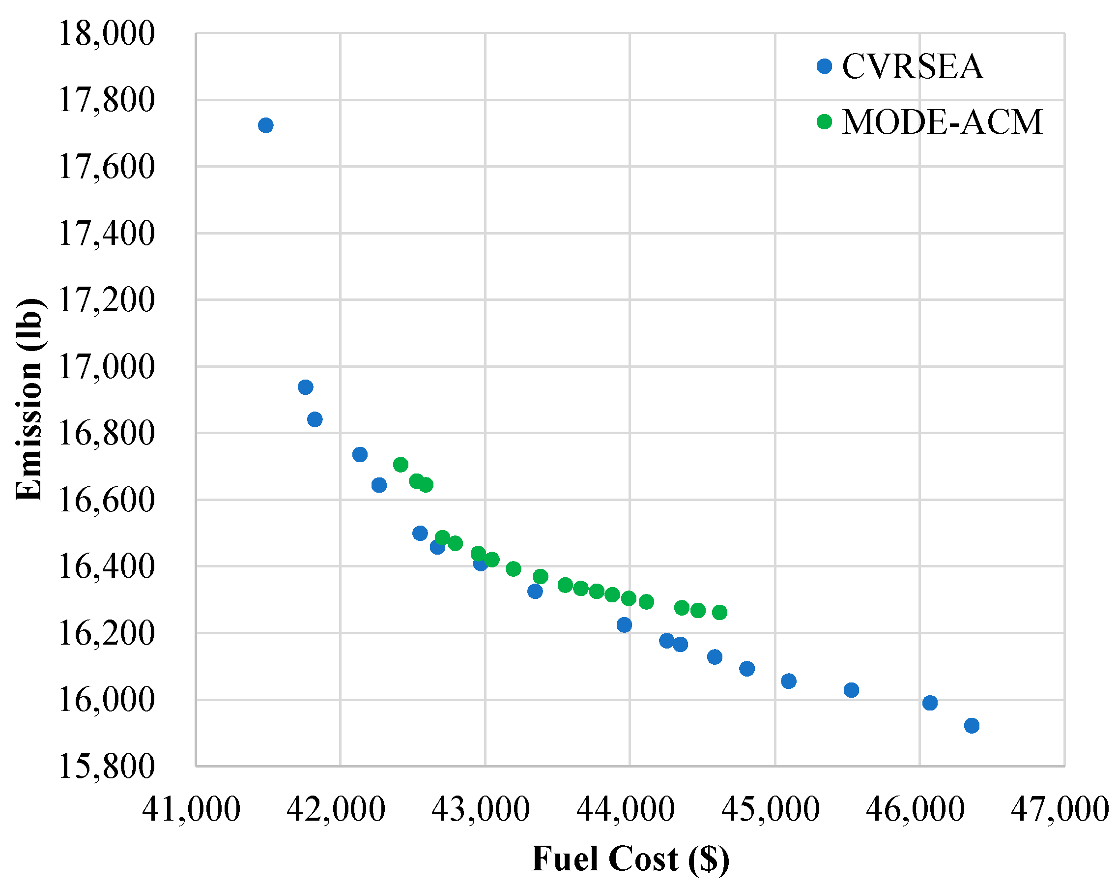
The Pareto fronts obtained by the CVRSEA and MODE-ACM are shown in Figure 4, and the data for these schemes are listed in

Table 2. The optimal result obtained by the CVRSEA and MODE-ACM.

Scheme	MODE-ACM		CVRSEA
	Fuel Cost ($)	Emission (lb)	Fuel Cost ($)	Emission (lb)
1	42,417	16,706	41,485	17,723
2	42,432	16,688	41,623	17,527
3	42,479	16,672	41,659	16,980
4	42,529	16,656	41,760	16,938
5	42,590	16,645	41,825	16,841
6	42,609	16,523	41,968	16,822
7	42,650	16,500	42,001	16,733
8	42,705	16,486	42,136	16,735
9	42,793	16,469	42,268	16,644
10	42,870	16,455	42,408	16,556
11	42,952	16,439	42,551	16,499
12	43,046	16,421	42,672	16,458
13	43,125	16,407	42,834	16,431
14	43,196	16,393	42,970	16,409
15	43,289	16,382	43,150	16,360
16	43,382	16,370	43,345	16,326
17	43,474	16,358	43,569	16,292
18	43,553	16,344	43,960	16,225
19	43,660	16,334	44,254	16,177
20	43,770	16,326	44,346	16,166
21	43,878	16,315	44,585	16,129
22	43,991	16,304	44,707	16,143
23	44,113	16,294	45,095	16,056
24	44,249	16,286	45,248	16,045
25	44,357	16,276	45,529	16,029
26	44,470	16,268	46,172	15,991
27	44,619	16,262	46,359	15,922
28	44,724	16,253	46,501	15,949
29	44,842	16,249	47,049	15,883
30	44,962	16,242	47,872	15,829

. The figure illustrates that the majority of the solutions generated by the CVRSEA are more effective than those produced by the MODE-ACM. This evidence substantiates the assertion that the CVRSEA exhibits superior convergence compared to the MODE-ACM. In addition to the algorithm’s convergence, the diversity of the CVRSEA is superior to that of the MODE-ACM, as evidenced by the wider Pareto front obtained by the CVRSEA. The experimental result shows that our proposed CVRSEA algorithm is able to effectively solve the multi-objective operation problem of the hydro–thermal hybrid system, and has the ability to solve the operation problem of the wind–solar–hydro–thermal multi-energy complementary system.

4.3. Results of Multi-Energy Hybrid System

Following a comparative analysis of the CVRSEA and MODE-ACM, CVRSEA is implemented in the MOHS, with consideration given to the optimisation of the power peaks, economic efficiency and environmental impact. The parameters of the CVRSEA are set as follows: population size = 91, neighbourhood size = 20, archive set size = 60, mutation probability = 1/100, mutation distribution index = 20, number of generations = 2000. In this case, we incorporate the observed output of the wind and photovoltaic energy into the complementary system. The load on the electricity system is balanced by regulating the output of the hydropower and thermal power stations.

The Pareto fronts of the MOHS problem and the Pareto fronts of the problem without wind–solar energy are both illustrated in Figure 5. As can be observed from the figure, the incorporation of wind and PV energy into the power system results in significant reductions in the emission of pollutants by the system and in the thermal power generation cost. The ranges of the fuel costs and emissions of the Pareto fronts without wind–solar energy are 41,488~48,966 and 15,955~18,951, respectively. After the incorporation of wind and PV energy into the power system, the ranges of the fuel costs and emissions are reduced to 33,973~44,222 and 7918~9673, respectively. In terms of the variation coefficient, there is no significant difference in the range of CV values between the two models. The experimental result shows that the multi-energy complementary system can not only enhance the economic benefits but also mitigate the impact of the thermal power generation on the atmospheric environment. The operational stability of the power system is primarily contingent upon the peaking of loads by hydroelectric power plants.

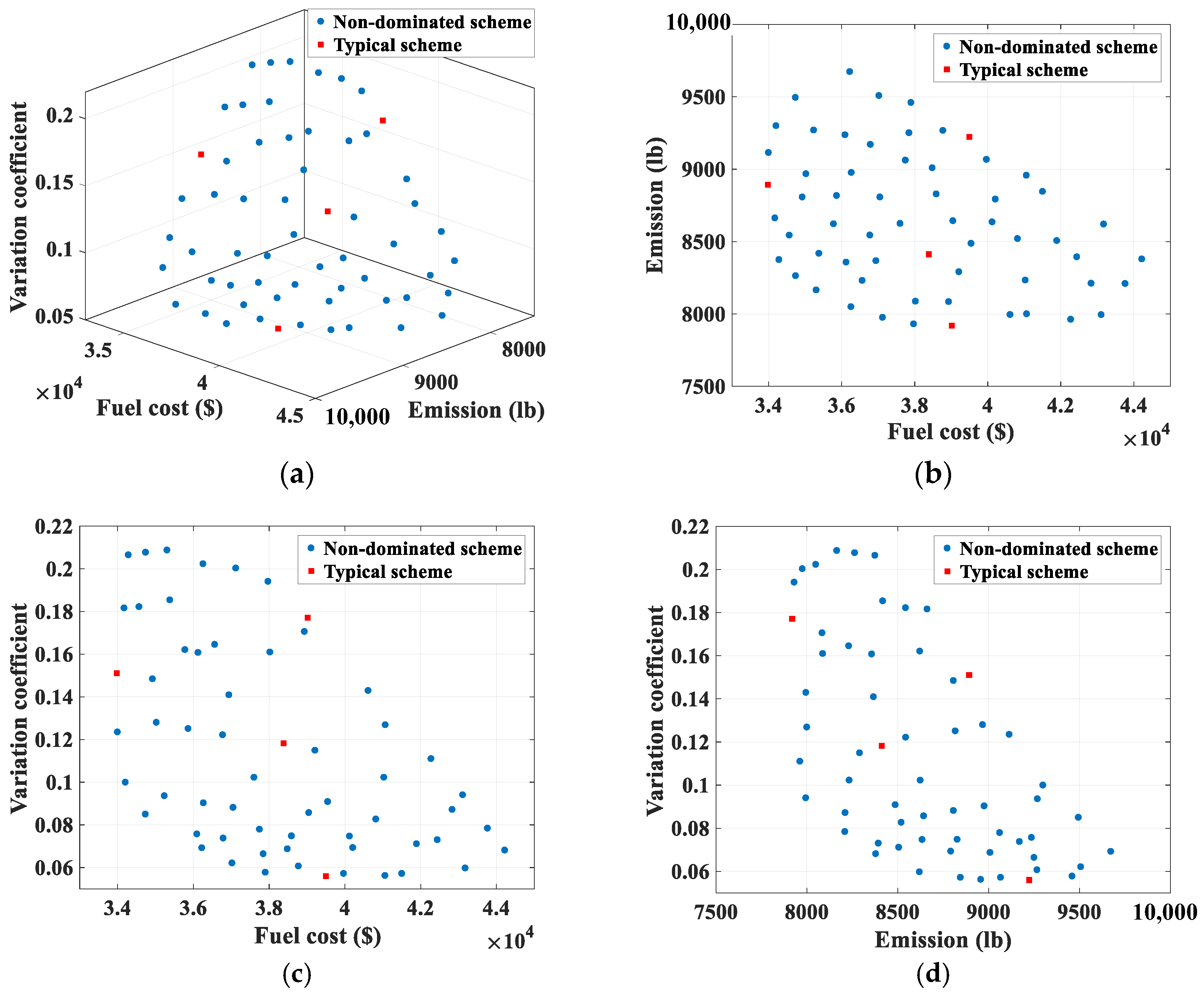
To show the scheduling process in detail, 4 typical schemes from 60 non-inferior solutions are selected to analyze and compare the effect of the multi-energy complementary system. Figure 6 shows the spatial locations of four typical schemes in the Pareto front, and the data for these schemes are listed in

Table 3. The optimal results obtained by the CVRSEA.

Scheme	Fuel Cost ($)	Emission (lb)	CV	Scheme	Fuel Cost ($)	Emission (lb)	CV
1	33,974	8893	0.151	31	37,901	9460	0.058
2	33,997	9114	0.123	32	37,972	7930	0.194
3	34,173	8662	0.182	33	38,023	8087	0.161
4	34,206	9299	0.100	34	38,384	8413	0.118
5	34,285	8375	0.206	35	38,484	9009	0.069
6	34,567	8543	0.182	36	38,593	8828	0.075
7	34,735	9495	0.085	37	38,775	9267	0.061
8	34,741	8263	0.208	38	38,933	8084	0.171
9	34,923	8807	0.148	39	39,019	7919	0.177
10	35,024	8968	0.128	40	39,049	8643	0.086
11	35,236	9269	0.094	41	39,213	8290	0.115
12	35,305	8165	0.209	42	39,497	9222	0.056
13	35,380	8418	0.185	43	39,548	8487	0.091
14	35,779	8622	0.162	44	39,967	9067	0.057
15	35,863	8817	0.125	45	40,123	8635	0.075
16	36,095	9237	0.076	46	40,211	8792	0.069
17	36,125	8357	0.161	47	40,615	7995	0.143
18	36,225	9673	0.069	48	40,819	8520	0.083
19	36,257	8049	0.202	49	41,030	8233	0.102
20	36,266	8976	0.090	50	41,060	8957	0.056
21	36,565	8231	0.165	51	41,068	8000	0.127
22	36,775	8544	0.122	52	41,504	8845	0.057
23	36,789	9170	0.074	53	41,893	8506	0.071
24	36,941	8367	0.141	54	42,276	7962	0.111
25	37,022	9508	0.062	55	42,442	8394	0.073
26	37,050	8807	0.088	56	42,834	8211	0.087
27	37,122	7975	0.200	57	43,111	7994	0.094
28	37,603	8624	0.102	58	43,177	8620	0.060
29	37,748	9062	0.078	59	43,766	8209	0.078
30	37,847	9251	0.066	60	44,223	8379	0.068

. These four typical scenarios are obtained using the Tchebycheff aggregation function according to the weights (1, 0, 0), (0, 1, 0), (0, 0, 1) and (0.333, 0.333, 0.333), respectively. From the figure and the table, typical scenario 1 (scheme 1) has the smallest fuel cost, typical scenario 2 (scheme 39) has the smallest emissions, typical scenario 3 (scheme 42) has the smallest CV value, and typical scenario 4 (scheme 34) is a multi-objective trade-off solution. Figure 7 shows the scheduling process details for the four typical schemes. It is clear from the figure that the remaining load process for typical scheme 3 tends to be a straight line, the remaining load process is more volatile for typical schemes 1 and 2 and the process is relatively less volatile for typical scheme 4. This result shows that by optimising the power peaking objective, it is possible to make the remaining load process for the power system stable, which allows thermal power to act as the base load of the power system and reduces the variability of the thermal loads.

The scheduling evaluation indicators include the fuel cost, emissions, CV value, total thermal power, total hydropower, total solar power, total wind power and total load of 4 typical schemes, which are displayed in

Table 4. The scheduling evaluation indicators for the four typical schemes.

Scheme	Fuel Cost ($)	Emissions (lb)	CV	Sum PT	Sum Ph	Sum Ps	Sum Pw	Total Load
Typical 1	33,974	8893	0.151	9372	10,079	1138	2061	22,650
Typical 2	39,019	7919	0.177	9209	10,241	1138	2061	22,650
Typical 3	39,497	9222	0.056	9812	9638	1138	2061	22,650
Typical 4	38,384	8413	0.118	9420	10,030	1138	2061	22,650

. From the table, we can see that although typical scheme 3 has the minimum CV value, the total thermal power is higher than for the other typical schemes. Typical schemes 1 and 2 may use fewer fossil fuel materials but the CV values are too high and may affect the stability of the power system’s operation. Typical scheme 4 is a trade-off solution, which can maintain the stable operation of the power system without incurring excessive costs and causing environmental pollution.

4.4. Impacts of Uncertainty

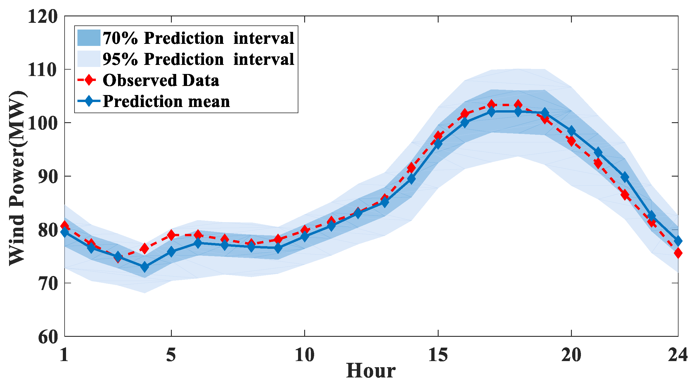
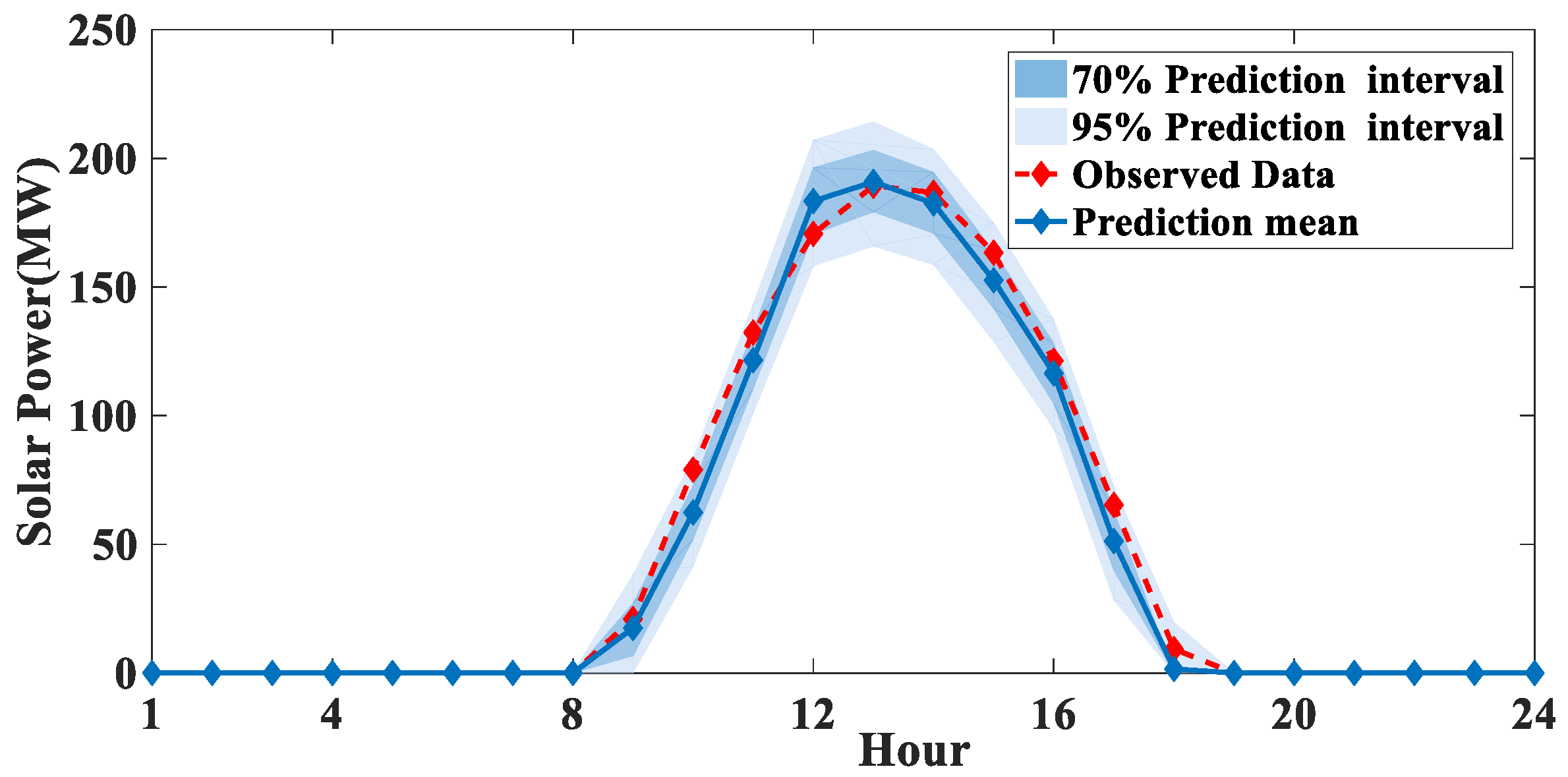
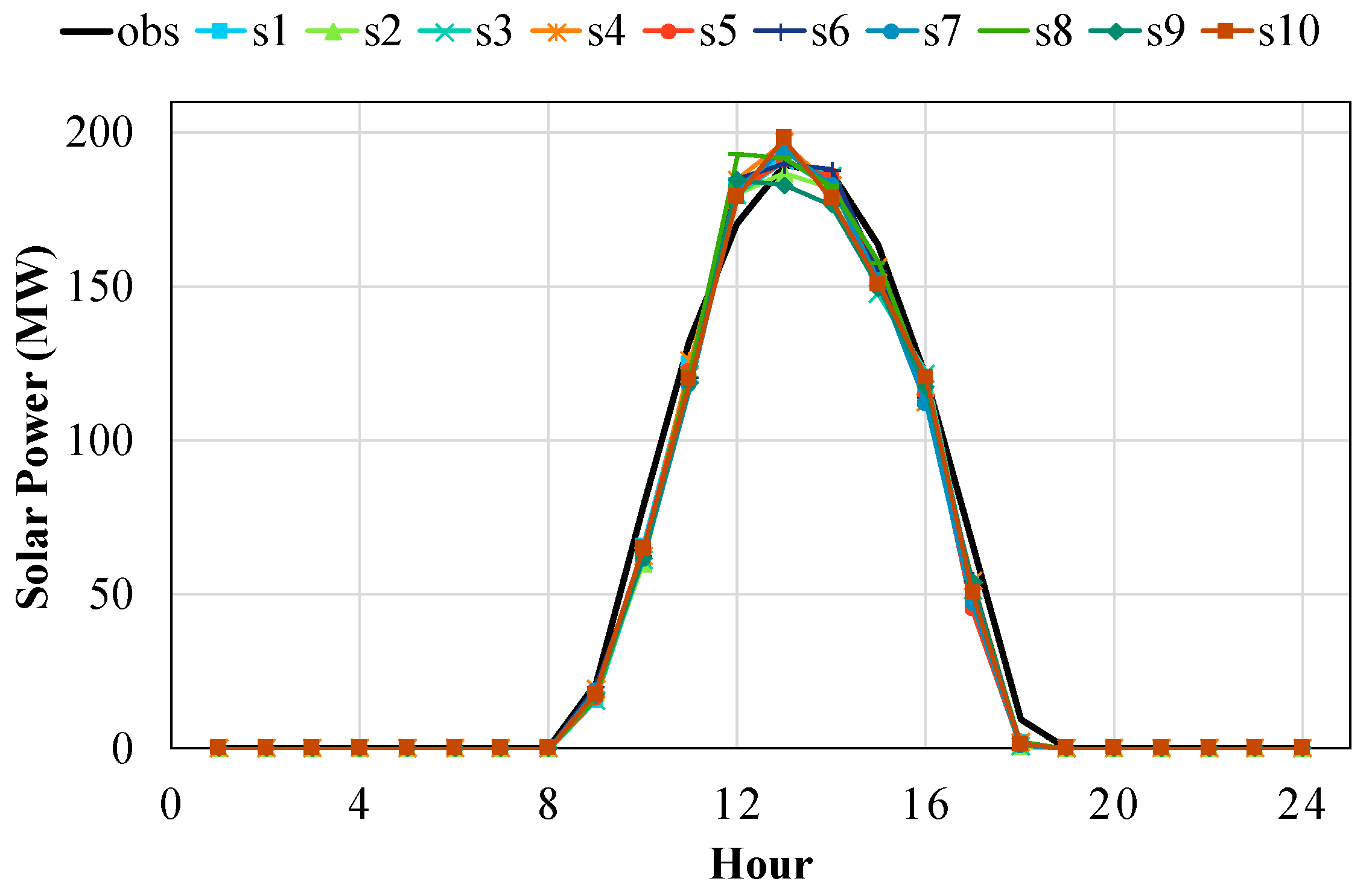
According to the uncertainty analysis and scenario simulation technology mentioned in Section 2.3, wind power and solar power uncertainty can be expressed using HMR. The Monte Carlo simulation method is used to simulate wind power and solar power fluctuations by generating 2000 scenarios. Subsequently, the k-medoids algorithm is employed to identify 10 representative post-cut scenarios out of 1000 cases. The mean and intervals of the wind power and solar power scenarios generated using HMR over 24 h are displayed in Figure 8 and Figure 9, respectively. The observed and forecasted wind power and solar power values are presented in

Table 5. The observed and forecasted wind power and solar power values.

Time (h)		1	2	3	4	5	6	7	8	9	10	11	12
Wind power (MW)	obs	81	77	75	76	79	79	78	77	78	80	81	83
	fore	80	77	75	73	76	77	77	77	77	79	81	83
Solar power (MW)	obs	0	0	0	0	0	0	0	0	21	79	132	171
	fore	0	0	0	0	0	0	0	0	17	62	122	183
Time (h)		13	14	15	16	17	18	19	20	21	22	23	24
Wind power (MW)	obs	86	92	97	102	103	103	101	97	92	87	81	76
	fore	85	90	96	100	102	102	102	98	94	90	83	78
Solar power (MW)	obs	189	187	163	121	65	9	0	0	0	0	0	0
	fore	191	183	153	116	51	2	0	0	0	0	0	0

. The 10 typical scenarios are illustrated in Figure 10 and Figure 11, where the scenarios are represented by s1 through s10, respectively.

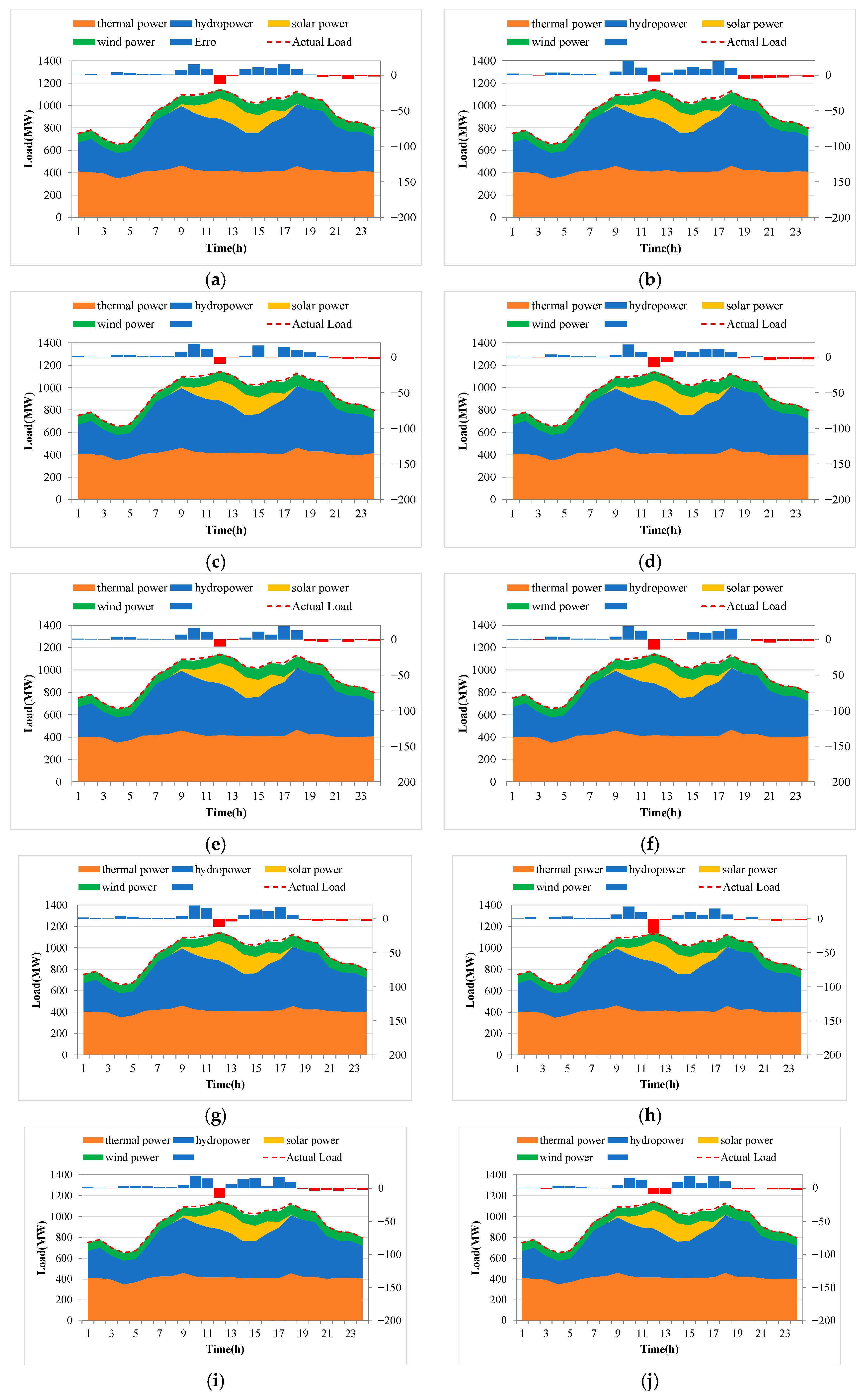
Each scenario comprises 24 h of wind power data and 24 h of solar power data for a multi-objective operation model of the hybrid system. Subsequently, the CVRSEA algorithm is employed to solve the aforementioned 10 typical scenarios, thereby obtaining the non-inferiority front in each scenario, as illustrated in Figure 12. From Figure 12, it can be seen that the Pareto front for each scenario is slightly different due to the uncertainty in the forecast but the overall shape of the front and range of the objective values are relatively similar. Figure 13 shows the scheduling process details of the 10 scenarios and also displays the system power errors caused by the differences between the forecast output and actual output. The system power errors are the differences between the load demand and the total load of the power system after integrating the observed wind and PV energy generation values, and the larger the system power error, the worse the negative impact on the operational stability of the hybrid power system. As can be seen from the icons, the errors range from −21 to 20, with larger errors between 09:00 and 19:00 than at other times of the day, making it more important to pay attention to the stability of the operation and meaning the system needs to reserve enough backup power to cope with the load errors. Depending on the system error and the regulation capacity of the cascade hydropower plant, it may have sufficient capacity to cope with the system error at the existing grid-connected scale for wind and solar energy, although as the scale of wind and solar energy values increase, it may be necessary to consider other energy storage devices to regulate the peak and frequency of the electricity grid.

4.5. Results of a Realistic Model System Considering a Demand-Side Management Strategy

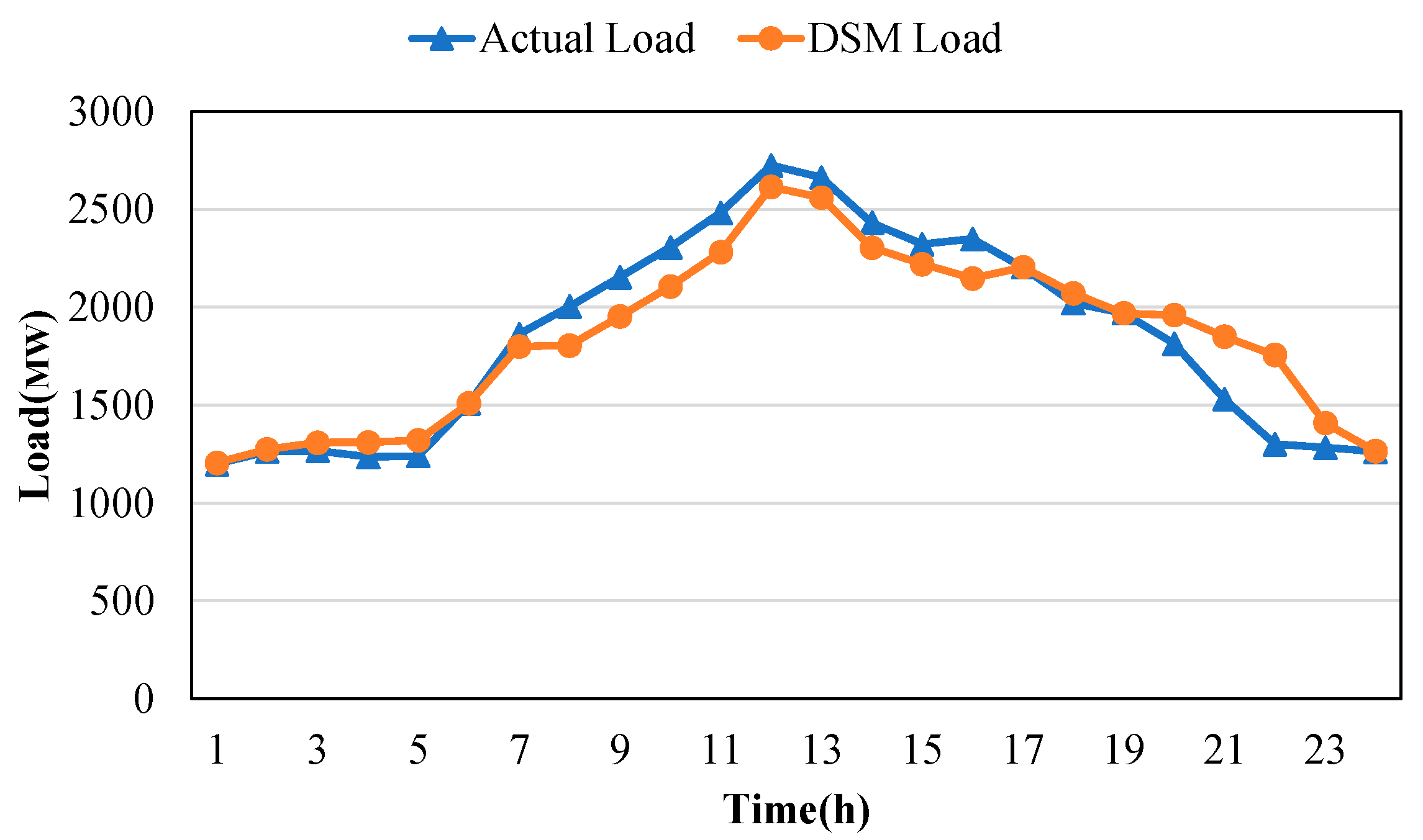
In order to validate our models and methods, the CVRSEA is applied to a realistic model of the wind–solar–hydro experimental base of the Yalong river basin in China. In this region, four wind farms, one solar farm and a hydropower station have been constructed. The four wind farms are designated Wodi (W1), Dahe (W2), Asa (W3) and Baiwu (W4). The solar farm in question is Zhalashan (S1). The reservoir is designated as Guandi (H1). The installed aggregate capacity of the four wind power stations (W1–W4) is 332 MW, distributed as 91.5 MW, 60 MW, 80 MW and 99 MW, respectively. The installed capacity values of S1 and H1 are 900 MW and 2400 MW, respectively. In addition, demand-side management strategies have a significant impact on the operation of the power system. Therefore, the optimal operation results considering demand-side management (DSM) strategies are also shown to demonstrate their effects. Figure 14 shows the load demand curve before and after DSM.

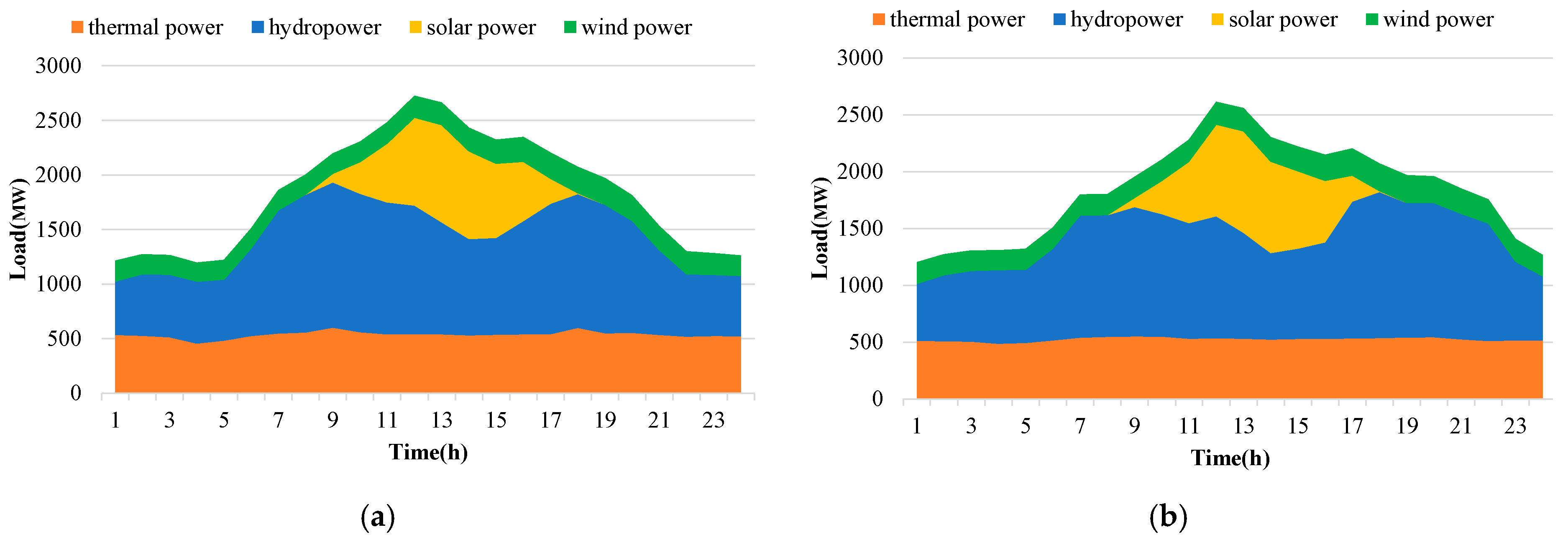
The CVRSEA is applied to the realistic model system, considering the power peak shaving, economic and environmental objectives. Typical scenarios with minimum CV values are selected to demonstrate the DSM performance. Figure 15 shows two typical scenarios with minimum CV values considering the DSM and without the DSM. The results show that through the demand-side management strategy, the peak value of the electricity load is reduced, which reduces the difficulty of the system’s peaking and frequency regulation and means the optimized thermal power generation is more stable, significantly enhancing the operational performance.

5. Conclusions

This paper has presented a multi-objective short-term operation model of a wind–solar–hydro–thermal hybrid system, which considers the power peak shaving, economic and environmental objectives. Furthermore, a cost value region search evolutionary algorithm was also proposed to solve the multi-objective model. From the experimental results, we can give the following conclusions: (1) the proposed algorithm outperforms the comparative algorithm in terms of algorithm convergence and Pareto front diversity when solving the multi-objective operation problem of the hydro–thermal hybrid system; (2) incorporating wind and solar energy into the power system increases the economic benefits of the power system and reduces the impact of the thermal power generation on the atmospheric environment; (3) the flexible regulating capacity of the hydroelectric plants allows them to effectively regulate peak loads, thereby increasing the stability of the electricity system; (4) the uncertainty of the wind and solar energy introduces operational errors into the system loads, while the flexible operation capability of the hydroelectric power plants allows them to effectively reduce the peak loads, thereby improving the stability of the power system; (5) as the scale of the wind and solar energy increases, the system needs to reserve enough backup power to cope with the load errors.

References

1. He, Q.; Tapia, F.; Reith, A. Quantifying the influence of nature-based solutions on building cooling and heating energy demand: A climate specific review. Renew. Sustain. Energy Rev. 2023, 186, 113660. [Google Scholar] [CrossRef]
2. Somoye, O.A. Energy crisis and renewable energy potentials in Nigeria: A review. Renew. Sustain. Energy Rev. 2023, 188, 113794. [Google Scholar] [CrossRef]
3. Walmsley, T.G.; Philipp, M.; Picón-Núñez, M.; Meschede, H.; Taylor, M.T.; Schlosser, F.; Atkins, M.J. Hybrid renewable energy utility systems for industrial sites: A review. Renew. Sustain. Energy Rev. 2023, 188, 113802. [Google Scholar] [CrossRef]
4. IRENA. Renewable Energy Statistics 2023; International Renewable Energy Agency: Masdar City, Abu Dhabi, 2023. [Google Scholar]
5. Nowdeh, S.A.; Naderipour, A.; Davoudkhani, I.F.; Guerrero, J.M. Stochastic optimization—Based economic design for a hybrid sustainable system of wind turbine, combined heat, and power generation, and electric and thermal storages considering uncertainty: A case study of Espoo, Finland. Renew. Sustain. Energy Rev. 2023, 183, 113440. [Google Scholar] [CrossRef]
6. Han, S.; He, M.; Zhao, Z.; Chen, D.; Xu, B.; Jurasz, J.; Zheng, H. Overcoming the uncertainty and volatility of wind power: Day-ahead scheduling of hydro-wind hybrid power generation system by coordinating power regulation and frequency response flexibility. Appl. Energy 2023, 333, 120555. [Google Scholar] [CrossRef]
7. Kharrich, M.; Selim, A.; Kamel, S.; Kim, J. An effective design of hybrid renewable energy system using an improved Archimedes Optimization Algorithm: Acase study of Farafra, Egypt. Energy Convers. Manag. 2023, 283, 116907. [Google Scholar] [CrossRef]
8. Bhandari, B.; Lee, K.-T.; Lee, C.S.; Song, C.-K.; Maskey, R.K.; Ahn, S.-H. A novel off-grid hybrid power system comprised of solar photovoltaic, wind, and hydro energy sources. Appl. Energy 2014, 133, 236–242. [Google Scholar] [CrossRef]
9. Chen, Q.; Tang, Z.; Lei, Y.; Sun, Y.; Jiang, M. Feasibility analysis of nuclear–coal hybrid energy systems from the perspective of low-carbon development. Appl. Energy 2015, 158, 619–630. [Google Scholar] [CrossRef]
10. Bao, X.; Li, F.; Sun, H.; Iglesias, G.; Shi, H. Performance characteristics and parameter analysis of a multi-DOF wave energy converter with hybrid power take-off systems. Energy Convers. Manag. 2023, 278, 116751. [Google Scholar] [CrossRef]
11. Al Afif, R.; Ayed, Y.; Maaitah, O.N. Feasibility and optimal sizing analysis of hybrid renewable energy systems: A case study of Al-Karak, Jordan. Renew. Energy 2023, 204, 229–249. [Google Scholar] [CrossRef]
12. Liu, Y.; Ye, L.; Qin, H.; Hong, X.; Ye, J.; Yin, X. Monthly streamflow forecasting based on hidden Markov model and Gaussian Mixture Regression. J. Hydrol. 2018, 561, 146–159. [Google Scholar] [CrossRef]
13. Liu, Y.; Qin, H.; Zhang, Z.; Pei, S.; Wang, C.; Yu, X.; Jiang, Z.; Zhou, J. Ensemble spatiotemporal forecasting of solar irradiation using variational Bayesian convolutional gate recurrent unit network. Appl. Energy 2019, 253, 13596. [Google Scholar] [CrossRef]
14. Li, F.-F.; Qiu, J. Multi-objective optimization for integrated hydro–photovoltaic power system. Appl. Energy 2016, 167, 377–384. [Google Scholar] [CrossRef]
15. Zhang, Z.; Qin, H.; Liu, Y.; Wang, Y.; Yao, L.; Li, Q.; Li, J.; Pei, S. Long Short-Term Memory Network based on Neighborhood Gates for processing complex causality in wind speed prediction. Energy Convers. Manag. 2019, 192, 37–51. [Google Scholar] [CrossRef]
16. Yaghoubirad, M.; Azizi, N.; Farajollahi, M.; Ahmadi, A. Deep learning-based multistep ahead wind speed and power generation forecasting using direct method. Energy Convers. Manag. 2023, 281, 116760. [Google Scholar] [CrossRef]
17. Liu, Y.; Qin, H.; Zhang, Z.; Pei, S.; Jiang, Z.; Feng, Z.; Zhou, J. Probabilistic spatiotemporal wind speed forecasting based on a variational Bayesian deep learning model. Appl. Energy 2020, 260, 14259. [Google Scholar] [CrossRef]
18. Liu, Y.; Hou, G.; Huang, F.; Qin, H.; Wang, B.; Yi, L. Directed graph deep neural network for multi-step daily streamflow forecasting. J. Hydrol. 2022, 607, 127515. [Google Scholar] [CrossRef]
19. Qin, H.; Zhou, J.; Lu, Y.; Wang, Y.; Zhang, Y. Multi-objective differential evolution with adaptive Cauchy mutation for short-term multi-objective optimal hydro-thermal scheduling. Energy Convers. Manag. 2010, 51, 788–794. [Google Scholar] [CrossRef]
20. Hamann, A.; Hug, G. Integrating Variable Wind Power Using a Hydropower Cascade. Energy Procedia 2016, 87, 108–115. [Google Scholar] [CrossRef]
21. Gong, Y.; Liu, P.; Ming, B.; Xu, W.; Huang, K.; Li, X. Deriving pack rules for hydro–photovoltaic hybrid power systems considering diminishing marginal benefit of energy. Appl. Energy 2021, 304, 117858. [Google Scholar] [CrossRef]
22. Li, H.; Liu, P.; Guo, S.; Ming, B.; Cheng, L.; Yang, Z. Long-term complementary operation of a large-scale hydro-photovoltaic hybrid power plant using explicit stochastic optimization. Appl. Energy 2019, 238, 863–875. [Google Scholar] [CrossRef]
23. Qi, Y.; Hu, W.; Dong, Y.; Fan, Y.; Dong, L.; Xiao, M. Optimal configuration of concentrating solar power in multienergy power systems with an improved variational autoencoder. Appl. Energy 2020, 274, 115124. [Google Scholar] [CrossRef]
24. Li, H.; Mahmud, M.A.; Arzaghi, E.; Abbassi, R.; Chen, D.; Xu, B. Assessments of economic benefits for hydro-wind power systems: Development of advanced model and quantitative method for reducing the power wastage. J. Clean. Prod. 2020, 277, 123823. [Google Scholar] [CrossRef]
25. Zhang, Z.; Qin, H.; Li, J.; Liu, Y.; Yao, L.; Wang, Y.; Zhou, J. Short-term optimal operation of wind-solar-hydro hybrid system considering uncertainties. Energy Convers. Manag. 2020, 205, 112405. [Google Scholar] [CrossRef]
26. Wang, Z.; Fang, G.; Wen, X.; Tan, Q.; Zhang, P.; Liu, Z. Coordinated operation of conventional hydropower plants as hybrid pumped storage hydropower with wind and photovoltaic plants. Energy Convers. Manag. 2023, 277, 116654. [Google Scholar] [CrossRef]
27. Liu, Y.; Zhan, X.; Lyu, H.; Qin, H. Region search evolutionary algorithm with constraint handling for multi-objective short-term wind-solar-hydro-thermal scheduling. E3S Web Conf. 2021, 233, 01018. [Google Scholar] [CrossRef]
28. Fan, J.-L.; Huang, X.; Shi, J.; Li, K.; Cai, J.; Zhang, X. Complementary potential of wind-solar-hydro power in Chinese provinces: Based on a high temporal resolution multi-objective optimization model. Renew. Sustain. Energy Rev. 2023, 184, 113566. [Google Scholar] [CrossRef]
29. Yang, T.; Ma, C.; Pérez-Díaz, J.I.; Patelli, E.; Liu, C.; Chen, D.; Xu, B. Identifying the functional form and operation rules of energy storage pump for a hydro-wind-photovoltaic hybrid power system. Energy Convers. Manag. 2023, 296, 117700. [Google Scholar] [CrossRef]
30. Ding, Z.; Fang, G.; Wen, X.; Tan, Q.; Mao, Y.; Zhang, Y. Long-term operation rules of a hydro–wind–photovoltaic hybrid system considering forecast information. Energy 2024, 288, 129634. [Google Scholar] [CrossRef]
31. Li, Y.; Ming, B.; Huang, Q.; Wang, Y.; Liu, P.; Guo, P. Identifying effective operating rules for large hydro–solar–wind hybrid systems based on an implicit stochastic optimization framework. Energy 2022, 245, 123260. [Google Scholar] [CrossRef]
32. Muhsen, D.H.; Ghazali, A.B.; Khatib, T. Multiobjective differential evolution algorithm-based sizing of a standalone photovoltaic water pumping system. Energy Convers. Manag. 2016, 118, 32–43. [Google Scholar] [CrossRef]
33. Das, I.; Dennis, J.E. Normal-boundary intersection: A new method for generating the Pareto surface in nonlinear multicriteria optimization problems. SIAM J. Optim. 1998, 8, 631–657. [Google Scholar] [CrossRef]
34. Liu, Y.; Qin, H.; Zhang, Z.; Yao, L.; Wang, C.; Mo, L.; Ouyang, S.; Li, J. A region search evolutionary algorithm for many-objective optimization. Inf. Sci. 2019, 488, 19–40. [Google Scholar] [CrossRef]
35. Yuan, J.; Liu, H.L.; Gu, F. A Cost Value Based Evolutionary Many-Objective Optimization Algorithm with Neighbor Selection Strategy. In Proceedings of the 2018 IEEE Congress on Evolutionary Computation (CEC), Rio de Janeiro, Brazil, 8–13 July 2018. [Google Scholar] [CrossRef]
Figure 1. Illustrations of regional division and identification.
Energies 17 04698 g001
Figure 2. Flowchart for the implementation of the CVRSEA to solve the problem.
Energies 17 04698 g002
Figure 3. Schematic diagram of the multi-energy complementary power generation system.
Energies 17 04698 g003
Figure 4. The Pareto fronts obtained by CVRSEA and MODE-ACM.
Energies 17 04698 g004
Figure 5. The Pareto fronts of the multi-energy hybrid system with and without wind–solar energy: (a) 3D objective scatter plot; (b) F2-F3 objective projection; (c) F2-F1 objective projection; (d) F3-F1 objective projection.
Energies 17 04698 g005
Figure 6. The Pareto fronts of the multi-energy hybrid system obtained by the CVRSEA: (a) 3D objective scatter plot; (b) F2-F3 objective projection; (c) F2-F1 objective projection; (d) F3-F1 objective projection.
Energies 17 04698 g006
Figure 7. The scheduling process details for the four typical schemes: (a) typical scenario 1; (b) typical scenario 2; (c) typical scenario 3; (d) typical scenario 4.
Energies 17 04698 g007
Figure 8. The mean and intervals of the wind power scenarios generated using HMR.
Energies 17 04698 g008
Figure 9. The mean and intervals of the solar power scenarios generated using HMR.
Energies 17 04698 g009
Figure 10. Typical wind power scenarios.
Energies 17 04698 g010
Figure 11. Typical solar power scenarios.
Energies 17 04698 g011
Figure 12. The Pareto fronts of the 10 scenarios (s1~s10) obtained by the CVRSEA.
Energies 17 04698 g012
Figure 13. The scheduling process details and system power errors for the 10 scenarios: (a) s1; (b) s2; (c) s3; (d) s4; (e) s5; (f) s6; (g) s7; (h) s8; (i) s9; (j) s10.
Energies 17 04698 g013
Figure 14. Load demand curve before and after DSM.
Energies 17 04698 g014
Figure 15. Typical scenarios with minimum CV values without the DSM and considering the DSM: (a) typical scenarios without DSM; (b) typical scenarios considering the DSM.
Energies 17 04698 g015