Article

The Effect of Increasing Aggregation Levels of Electrical Consumption Data on Renewable Energy Community (REC) Analyses

by
Marco Raugi
1,2,
Valentina Consolo
1,*,† and
Roberto Rugani
1,*,†
1
Department of Energy, Systems, Territory and Constructions Engineering, University of Pisa, L.go Lucio Lazzarino 1, 56122 Pisa, Italy
2
UNESCO Chair on “Sustainable Energy Communities”, University of Pisa, L.go Lucio Lazzarino 1, 56122 Pisa, Italy
*
Authors to whom correspondence should be addressed.
These authors contributed equally to this work.
Energies 2024, 17(18), 4647; https://doi.org/10.3390/en17184647
Submission received: 22 July 2024 / Revised: 10 September 2024 / Accepted: 13 September 2024 / Published: 18 September 2024

Abstract

:
The growing number of renewable energy communities (RECs) exemplifies the potential of citizen-driven actions towards a more sustainable future. However, obtaining hourly measured consumption data from REC members remains challenging, hindering accurate feasibility studies for the development of communities. This study examines the impact of estimating hourly consumption from aggregated data on REC analysis results. A case study with real consumption data from diverse users, representative of a typical community in Tuscany, Italy, was analysed to investigate various influencing factors. Multiple scenarios were simulated: two open-source tools estimated energy production from the community’s PV plants, and two REC configurations were considered—one with consumers and prosumers and another with consumers and a producer (with the same total installed power). Additionally, three locations were evaluated to consider the importance of geographical positioning. The study revealed that the impact of consumption data aggregation is more significant in scenarios with low energy sharing, such as the scenario where prosumers were replaced with a producer. Geographical positioning showed no major discrepancies in energy and economic outcomes, implying that using estimated hourly consumption data from aggregated data has a relevant impact regardless of location. Furthermore, different weather files did not affect the impact of aggregated consumption data.

1. Introduction

The concept of renewable energy communities (RECs) is quite recent and brings with it promising prospects for building a greener future. A REC is a legal entity whereby citizens’ groups, organisations and enterprises can come together to produce and share renewable energy. So a REC can be described as an association whose members are consumers, producers or prosumers; prosumers are users who both use and produce energy from renewable sources. The production of green energy and its sharing among the members of the REC bring environmental, economic and social benefits to all of the members of the community. In the contemporary era, a considerable number of renewable energy communities are being financed globally. In Europe, there are a minimum of 3500 such sites [1], while in the USA, there are approximately 100 [2], and there are over 100 in Canada, Australia and New Zealand [3]. This increasing interest in RECs represents a promising way to increase the share of renewable energy in the global energy mix, contributing to decarbonisation and leading to a clean energy transition. Energy transition is nowadays of the utmost importance, and the academic community is focusing on different methods to promote it in the best way possible. For instance, since residents need both electricity and heat daily, residential buildings are characterized both by an electrical and a thermal load. Hence, they can be seen as multi-energy systems (MESs) (i.e., systems wherein multiple energy sectors interact with each other thanks to energy conversion processes). In recent years, more and more attention has been devoted to MESs by researchers who aim to improve integrated energy systems from environmental, economic and security points of view [4,5,6]. Another challenge related to the energy transition is the exploitation of the peculiar characteristics of diverse locations all around the world. Islands, for example, represent really interesting environments with specific needs and challenges to face as per the electricity distribution: in [7], the authors propose adaptive energy management to perform the optimal operation for the island group energy system. In this context, RECs can be seen as MESs themselves if they involve more than one energy source to power the community. And even if they are based on only one kind of power generator, they can always concretely contribute to a more sustainable future by valorising the unique characteristics of a specific place and exploiting them to reduce consumption and increase energy production from renewable sources.
The creation of a community is an action that can and should start from below: from citizens, local authorities or small businesses; hence, all these actors can become main characters, playing a major role in the future energy system. In order to conduct a comprehensive and accurate investigation into the behaviour of a REC, it is essential to perform simulations of the community with a high level of detail, at least on an hourly basis. It is therefore necessary to estimate the energy production by renewable sources (according to [8], photovoltaic (PV) panels are the most common renewable energy source) and the energy consumption by users on an hourly basis. As for the first quantity, nowadays there are many researchers dealing with the forecasting of energy production from renewable sources [9,10,11]. Furthermore, a number of tools are available for estimating the hourly energy production from PV or wind systems, like EnergyPlus, Renewables.Ninja, PVGIS and TRNSYS. Conversely, it is often challenging to obtain hourly measured data on energy consumption by users. A number of studies have been conducted with the objective of identifying the characteristics of electricity consumption in both residential [12,13] and industrial contexts [14,15]. These studies are valuable instruments for the examination of the resilience and robustness of the energy grid as well as for the conceptualisation phase of a power plant designed to feed certain kinds of users. Nevertheless, they are unable to align perfectly with the distinctive characteristics of a particular pre-existing real-world scenario, such as the one exemplified by a flourishing energy community.
In the context of a local community that aspires to establish a REC, it is essential to undertake a detailed examination of the peculiar features of their electrical consumption patterns and behaviours. The issue is that in the majority of instances, hourly measured electrical consumption data are not readily accessible. This phenomenon is due to different factors. Firstly, not all utilities are yet equipped with the latest generation of electronic electricity meters, so for some users, only aggregated consumption measures are available. Secondly, it is quite common that the establishment of a REC is promoted by a single individual or legal entity: they take charge of collecting the consumption data of all the various possible members but do not have direct access to their data. Hence, they must tackle the issue with only the data provided, which are frequently presented at a high level of aggregation. Finally, when it is possible to collect data directly from the source, the problem is that the main source is represented by electricity bills, which provide only monthly consumption or monthly consumption divided by time bands. As a matter of fact, in order to have access to their hourly electricity consumption data, users must undertake a procedure that is not automatic because it requires registration on the website of their local distribution system operator. Not only may this procedure be difficult for some people, like the elderly ones, but it is also often unknown because it is not necessary for connection to the electricity grid. Hence, there are many people who are unaware of the possibility of controlling deeply in detail their electrical consumption. This illustrates the necessity for an information campaign on these issues, with the objective of enhancing the energy awareness of the majority of citizens. Given this, we are often limited to the availability of consumption data that have been grouped according to different levels of aggregation (annual consumption data, monthly consumption data or monthly consumption data divided by time bands). A deeper level of detail, such as that of a quarter of an hour, would enhance the alignment between production and consumption. Nevertheless, the acquisition of consumption data at the quarter-hour level remains a significant challenge, despite the gradual proliferation of smart meters with the capacity to record data in such increments. This obstacle is compounded by the generic nature of photovoltaic production simulation software, which typically operates with hourly output. In [16], a technique to determine the hourly energy profile of a user from their monthly energy bills is proposed and validated. This method could be really useful when monthly consumption data divided by time bands are available. In this work, however, our purpose is to quantify the impact of using aggregated data not only at that level of aggregation but also at higher levels of aggregation, like monthly or annual ones.
As a result of our collaboration with a number of public institutions and local associations, we were able to undertake a few in-depth investigations of some real case studies of Italian RECs under development: the availability of hourly consumption data for each user enabled a high level of accuracy in the studies. Moreover, consumption data were categorised into increasingly aggregated levels in order to replicate the common scenarios that may be encountered in the analysis of a rising REC. One representative case study has been presented in [17]: the present work is intended to build upon the findings of this previous study by incorporating additional factors that may impact the results of the analysis of a REC. The case study presented in this paper deals with a REC that is exemplary of a typical community in Tuscany (a region in the centre of Italy). The representative case was realized using electrical consumption data obtained from real users of different types, and its location was chosen to be in the town of Pisa. The REC is composed of consumers and prosumers, while the participation of producers is not considered at first. Subsequently, in order to deeply investigate the impact of using aggregated consumption data in REC simulations, we decided to develop a second scenario wherein all the prosumers were replaced by pure consumers and all their PV plants were replaced by a unique producer. In this way, we were able to investigate the discrepancies between the outputs of these two cases. Moreover, we wanted to broaden the research topic and also focus on the differences that can be highlighted when using two different tools to estimate the energy production of PV systems. That is why we chose to estimate it through two of the main open-source tools for this purpose: EnergyPlus and Renewables.Ninja. This way, we have four cases in total: two for the original REC with no producers, adopting EnergyPlus for one instance and Renewables.Ninja for the second instance for the estimation of the energy production, and two for the modified REC with no prosumers and one producer, again exploiting EnergyPlus for one instance and Renewables.Ninja for the second instance for the estimation of the energy production. Finally, we widened the investigation one last time to deal with the influence of the geographical positioning of the REC. We supposed moving the community to a different location while maintaining the same configuration of users, prosumers and producers and the same production-to-consumption ratio. We chose two exemplary towns, i.e., Palermo and Milano, placed in the south and in the north of Italy respectively. Now we deal with a total amount of twelve cases, since there are four of them for each town. This paper aims to undertake a comparative analysis of the results derived from simulating the behaviour of a REC using actual hourly consumption data with those obtained from simulations using aggregated data to estimate hourly shared energy for the same REC. Hence, the paper aims to answer the following research questions:
  • What is the impact of using hourly data estimated from aggregated data for the analysis of a REC? Does this impact vary if the configuration of the REC itself undergoes a change?
  • Dealing with this impact, what discrepancies emerge when employing two different tools to evaluate PV energy production?
  • Does the effect of using estimated hourly data change if the geographical location of the community varies?

2. Materials and Methods

This work focuses on the analysis of a case study of a representative REC and covers both the technical and the economic aspects of the community. A multitude of scenarios were subjected to analysis. As previously stated, two tools for estimating energy production and three locations were considered in conjunction with the prosumer/producer scenarios, resulting in a total of twelve cases under investigation. However, it must be highlighted that each of these cases has been subjected to four distinct simulations. The initial simulation employed actual hourly measured consumption data as the input, while the subsequent three simulations utilised hourly data estimated from three datasets with progressively increasing levels of aggregation. In particular, the three aggregated datasets considered are as follows: monthly consumption divided by time bands, monthly consumption, and annual consumption. Consequently, a total of forty-eight cases have been simulated. The methodology adopted for each of the simulated cases can be summarized as follows:
  • The input dataset was compiled using actual hourly measured electrical consumption data from real users considered as community members. This dataset represents the hourly scenario (H). Section 2.1 provides a comprehensive description of the real case study under investigation.
  • The dataset H was processed three times by employing three distinct approaches with the purpose of obtaining three datasets with increasing levels of aggregation: monthly consumption data divided according to Italian time bands (M–B) (as illustrated in Figure 1 [18,19]), monthly consumption data (M–A) and annual consumption data (A). As a result, four scenarios were set up.
  • For each group of aggregated data, a proportional distribution was employed in order to estimate the corresponding hourly data. No assumptions were made in the process of dividing the consumption; instead, a purely mathematical spread was employed. Details regarding the process through which we estimated hourly consumption starting from aggregated data are provided in Section 2.2.
  • Exploiting a MATLAB R2023b code we developed, we ran the simulations for each of the four scenarios, focusing on both energetic and economic aspects of the community. Section 2.4 illustrates the methodology used for the calculation of the results.
  • Ultimately, the outcomes from case H were employed as a point of reference for a comparative analysis of the four distinct cases.
Figure 2 illustrates the methodology flowchart employed in this study. The objective of this paper is to quantify the impact of considering electrical consumption data at varying levels of aggregation as simulation inputs for the analysis of the same REC. As electricity consumption data are often available only in aggregated forms, it is important to recognise the loss of accuracy that this aggregation introduces.
This section is organized as follows: Firstly, the analysed case study is described in deep detail in Section 2.1. Secondly, Section 2.2 deals with the methodology adopted to treat the hourly measured consumption in order to realize the three different scenarios of estimated hourly consumption, starting from datasets with increasing levels of aggregation. Thirdly, Section 2.3 focuses on the estimation process of the energy generated by the community PV plants. As previously stated, this estimation was made two times using two different open-source tools: EnergyPlus and Renewables.ninja [20]. Finally, Section 2.4 provides a comprehensive description of the MATLAB R2023b code adopted to run the simulations of the community for the computation of all the energetic and economic quantities.

2.1. The Case Study

The case study on which the analysis focuses is of an exemplary REC located in Pisa, which is a town in Tuscany. Tuscany is a region in central Italy where many people are enthusiastic to be involved in collective actions, and it is quite common for ambitious projects to be realized in a bottom-up fashion. In recent years, the creation of different RECs was often the result of a strong desire expressed by small groups of citizens. It is not infrequent that a little group of families started the process, becoming promoters of a citizen-driven energy action. These families may decide to participate in the REC as users or prosumers with their houses, but they also may involve a local volunteer association in the project. In this way, local charities may participate as well. In some cases, it also happened that medium-sized companies also became aware of the project and decided to join the community with the buildings that were their premises. Some projects were eventually proposed to the the municipality, which agreed to participate through public buildings such as offices and schools. This showed that some RECs may arise as the result of a bottom-up action for a more sustainable future.
For the realization of the present case study, we chose to consider 20 electricity delivery points (PODs) between consumers and prosumers. The concept of the prosumer is a relatively recent addition to the landscape of energy consumption. These individuals are not only end-users of electricity but also possess their own generation facilities, which utilise renewable energy sources. The energy generated is utilised for self-consumption, with any surplus shared with other members of the community [21,22,23]. The participation of producers is not considered at first. Nonetheless, as previously mentioned, the authors decided to study a second scenario wherein all the producers have been replaced by pure consumers and all of their PV plants have been replaced by a unique producer. There are no differences in the production-to-consumption ratio between the two cases since the producer’s PV plant has been sized with an installed PV capacity equal to the total installed PV capacity of all the prosumers. In this way, it is possible to investigate the discrepancies between the outputs of the simulations of these two cases. The next paragraphs provide a detailed description of the case characterized by the presence of only consumers and prosumers.
Fourteen users of the REC can be identified as consumers. They are: seven family apartments, a building intended for both residential and commercial use, three condominiums for homeless people and three office buildings.
Six users of the REC can be identified as prosumers. They are: the town hall, three public primary schools, a local charity building where a canteen for homeless people takes place and the premises belonging to a medium-sized enterprise. All of these buildings are flat-roofed, and they are characterized by different surfaces available for the installation of PV panels. The available surfaces on the roofs are: 900 m2 for the town hall, 900 m2, 200 m2 and 200 m2 for the three primary schools, 400 m2 for the local charity building with the canteen and 400 m2 for the company building. Given that the panels are to be mounted at a slope angle of 35°, approximately half of the available surfaces must be reserved to accommodate the installation and subsequent maintenance of the PV panels. It is assumed that the efficiency of the panel is approximately 20% [24]. Then, the peak PV power that is going to be installed is: 90 kWp (town hall), 90 kWp, 20 kWp, 20 kWp (schools), 40 kWp (canteen) and 40 kWp (enterprise), leading to a total peak power of 300 kWp installed by the prosumers.

2.2. Consumption Data Processing

We had at our disposal the real hourly electrical consumption data of the users who are supposed to take part in the REC. This consumption was measured hour-by-hour during the whole year of 2022. Since the total amount of users and prosumers of the community is 20, the dataset can be described as a 8760 × 20 matrix (number of hours per year × number of users+prosumers). This matrix represents the real consumption scenario of the community. For the sake of clarity, it will henceforth be referred to as the H scenario. We processed data from the H scenario three times with three different approaches in order to obtain three datasets with increasing levels of aggregation: monthly consumption data divided according to Italian time bands (as illustrated in Figure 1), monthly consumption data and annual consumption data. These aggregated datasets correspond to the possible consumption data that end-customers have at their disposal based on the information given to them by their local electricity supplier. We decided to realize these three datasets in order to recreate the most common real-life situations that a designer may face. Then, for each group of aggregated data, we distributed them proportionally to estimate the corresponding hourly data. As a result, three new scenarios were established: M–B, M–A and A. The M–B scenario is the dataset of estimated hourly consumption obtained from monthly consumption data divided by time bands, the M–A scenario is the dataset of estimated hourly consumption obtained from monthly aggregated consumption data, and A is the dataset of estimated hourly consumption obtained from annual consumption data.
Here follows the detailed description of how we obtained the A scenario, i.e., how we estimated hourly consumption starting from the most aggregated dataset: that is, the annual one. As for the others, we followed the very same procedure and skipped the unnecessary steps. For the sake of clarity, Table 1 summarizes the symbols used in the following paragraphs.
Annual consumption data of a single user can be represented with the scalar A. In order to estimate the corresponding hourly consumption, no assumptions on the users’ behaviour were made; instead, a purely mathematical spread was employed by following the steps below:
  • Estimation of the monthly consumption:
    For each month, we computed the ratios between the number of days of the month and the number of days of the year:
    r m = d m d y
    where m goes from 1 (January) to 12 (December). Hence, d m could be equal to 31, 30, or 28, while d y is equal to 365. Secondly, we built r , which is the 12 × 1 vector containing all of the ratios:
    r = r 1 r 12
    Then, we built the 12 × 1 monthly consumption vector l m by simply multiplying r by the scalar A, with A representing the annual consumption:
    l m = r · A
  • Estimation of the monthly consumption divided by time bands:
    This estimation is based on the number of hours contained in each time band in each month. Firstly, we calculated the number of hours h m in each month, where m goes from 1 (January) to 12 (December). Secondly, for each month, we calculated the three ratios between the number of hours of each time band and the number of hours of the month itself. Hence, for each month, we have three values of r b , m , where b stands for time band and goes from 1 (F1) to 3 (F3), and m stands for hours of the month. Then, we built the 12 × 3 matrix R b m containing all the values of r b , m :
    R b m = r 1 , 1 r 2 , 1 r 3 , 1 r 1 , 12 r 2 , 12 r 3 , 12
    Then, we built the 12 × 3 matrix L m b consisting of the monthly consumption divided by the time bands by simply multiplying l m by R b m :
    L m b = l m · R b m
  • Estimation of the hourly consumption:
    First, we built H b , which is a 36 × 8760 matrix containing elements that can be equal only to 1 or to 0. The first three rows of the matrix are related to January, rows 4 to 6 are related to February, and so on. Among the three rows related to a month, the first one is related to the first time band (F1), the second one is related to the second time band (F2), and the third one is related to the third time band (F3). Hence, the element H b i , j represents the hour j of the appropriate month, and it is equal to one if belongs to the appropriate time band indicated by the row; otherwise, it is null.
    H b = H b 1 , 1 H b 1 , 8760 H b 36 , 1 H b 36 , 8760
    For instance, the elements H b 1 , j and the elements H b 2 , j for j = 1:24 are equal to 0 since the first day of the year is always festive. Coherently, the elements H b 3 , j for j = 1:24 are equal to 1 because all of the hours of the 1st of January belong to the third time band F3.
    Secondly, we computed H b 1 , which is the 8760 × 36 psuedoinverse matrix of H b .
    Then, we reshaped the monthly consumption divided by time bands matrix L m b into the 36 × 1 vector l m b .
    Finally, we multiplied H b 1 by l m b , thus obtaining the 8760 × 1 vector of estimated hourly consumption l h :
    l h = H b 1 · l m b
These steps summarize the process we adopted to estimate hourly consumption data of a user starting from their annual consumption. As previously mentioned, when dealing with the estimation of hourly consumption data starting from less aggregated data, we followed the very same procedure, skipping the unnecessary steps. That means that we performed steps 2 and 3 when starting from monthly data and only step 1 when starting from monthly data divided by time bands. It is important to note that the described process results in a loss of information, as depicted in Figure 3. The graph shows how the higher the level of aggregation, the more significant the loss of information and the flattening of the results. All of the graphs related to all of the users considered for the proposed case study are available in Appendix A. Finally, it is worth highlighting that our model could be described as an agnostic one, since no specific information related to the users’ behaviour was used in the estimation of their hourly consumption, but a purely mathematical spread was adopted. This choice, compared with the ones in other works (e.g., [16]), represents a more general approach to the problem. This feature allowed us to achieve interesting findings that can be particularly useful in all of those cases where a designer does not have at their disposal detailed information on the consumption behaviour of the members of a REC under analysis.

2.3. Production

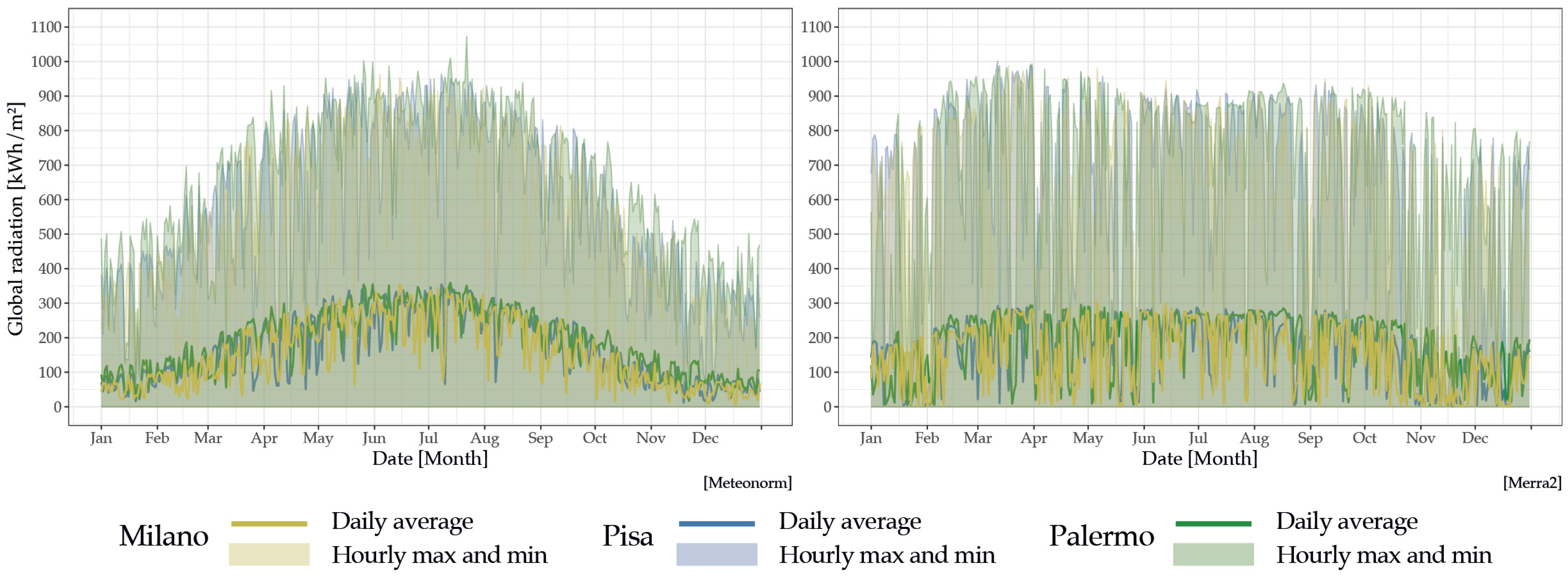
The case study we focused on is located in the city of Pisa. However, considering the significance of testing a building under diverse climatic conditions with contrasting trends, we decided to perform the simulations using weather conditions of three Italian cities: Milano, Pisa and Palermo. This approach enabled us to comprehend the impact of external factors (such as temperature and radiation) on PV productivity and their influence on shared energy. The three cities were selected as test locations for the REC due to their distinctly different climate profiles, making them representative cases for a broader range of cities. Milano has a humid subtropical climate characterized by hot, humid summers and cold, foggy winters. Pisa, located in central Italy, experiences a Mediterranean climate with hot, dry summers and mild, wet winters. Palermo, in southern Italy, enjoys a warm Mediterranean climate featuring long, hot summers and mild, wet winters. Compared to Milano, Pisa and Palermo have milder winters, with Palermo being the warmest and driest of the three cities year-round. To demonstrate such differences in temperature and radiation trends, Figure 4 and Figure 5 show the outputs of the climatic files used for the simulations.
Two typical meteorological year (TMY) weather files, which are composed of 12 typical months of the full-time period available, were selected and downloaded from two databases:
  • Meteonorm, which is based on 19 years of observations (2000–2019);
  • MERRA-2 [25], which is based on 18 years of observations (2001–2019).
Despite them both being TMY files, the trends depicted in the variables show some differences. For instance, the temperature trends are very similar, as evidenced by R2 values of 0.75 for Milano and Palermo and 0.71 for Pisa using Meteonorm as the statistical baseline. However, the MERRA-2 weather file is much more flattened: lacking some peaks found in the Meteonorm weather file. Specifically, MERRA-2 has mean absolute errors (MAEs) of 3.3 °C for Milano and Pisa and 2.37 °C for Palermo. The magnitude of the global radiation is similar for both databases. However, Meteonorm displays a more bell-shaped curve for the three cities, while MERRA-2 shows a flatter peak trend. The R2 values are 0.42 for Milano, 0.50 for Pisa and 0.60 for Palermo. The MAEs experience quite high differences, such as 121 kWh/m2 for Milano and Pisa and 116 kWh/m2 for Palermo. Finally, the electricity production by the photovoltaic panels was simulated using EnergyPlus with the Meteonorm weather file and with Renewable.ninja [20] using the MERRA-2 climate file.

2.4. The Model

The REC’s behaviour was analysed by employing a MATLAB R2023b model. The model takes as input one year of hourly electrical consumption data of REC members and one year of hourly energy production generated by the community’s PV plants. The consumption input is composed of C , which is an N h o u r s × N u s e r s matrix, where N h o u r s is equal to 8760 and N u s e r s is the total number of PODs involved in the REC. Hence, N u s e r s is equal to 20 for the scenarios wherein only consumers and prosumers are considered and is equal to 21 for the scenarios wherein prosumers have been replaced by consumers and a producer has been added to the configuration. In both cases, C is realised by juxtaposing all column vectors representing the hourly consumption of each user. Similarly, the energy production input consists of another N h o u r s × N u s e r s matrix: E . These two matrices are ordered in the same way: that means that the i-columns of both matrix C and E refer to the same i-PODs of the community. With regard to matrix E, all of its columns that are related to users who are classified as pure consumers are null. For each hour, the model compares the energy consumption of each user, that is, the energy requested by the user themself, with the energy generated by the same user, if any:
Δ E , C = E : , i C : , i
Three distinct cases may occur:
  • Δ E , C < 0 : This case may occur under different circumstances. Firstly, if the POD belongs to a pure consumer, it does not produce its own energy, so Δ E , C is always negative. Otherwise, if the POD belongs to a prosumer, then a negative Δ E , C can mean two things: either their plant is not producing in the considered hour (e.g., during nighttime) or its plant is generating only a fraction of the requested energy. In all cases, the produced energy (if any) is not enough to satisfy the request from the user, so the value of Δ E , C represents the energy taken from the grid to cover the consumption.
  • Δ E , C = 0 : This case happens whenever there is a balance between the energy requested by the user and the energy produced by the user themself. Hence, it may happen only for those users classified as prosumers.
  • Δ E , C > 0 : This case is always verified for all the producers in a configuration, since producers do not consume energy. This case may also happen for a prosumer whenever they are generating more energy than they require. Obviously, it will never occur for a user, since a user is not able to produce their own energy and to have self-consumption. When Δ E , C is positive, its value represents the amount of energy fed into the grid and sold.
When the last case happens, it means that there is a certain amount of energy that can be virtually shared among the members of the REC. For each hour, then, the code computes the value of shared energy in accordance with the definition set forth by the Italian Regulatory Authority for Energy, Networks and Environment, which defines shared energy as the minimum, in each hour, between the sum of electricity actually fed in and the sum of electricity withdrawn through connection points that are relevant for the purposes of a renewable energy community [26].
Since Italian law [27] ruled that twenty years is the reference duration for Italian REC studies, and the Italian Energy Services Provider (GSE) has based all incentives and energy accounts on a twenty-year timeframe, using the MATLAB R2023b model, the authors computed all the energy-related quantities for twenty years of operation of the community. For the purposes of this work, as for the energetic quantities, only one year of operation would have been sufficient for the analysis. Nevertheless, the 20-year simulation becomes necessary if we want to assess an economic analysis, too. Some hypotheses have been settled to simulate the years following the first one: Firstly, as for the electrical consumption data, they are assumed to remain unchanged over the years. Of course, this hypothesis is not realistic, since energy consumption varies over time depending on many phenomena, like changes in users’ behaviour and variations in climatic conditions. However, since the purpose of this paper is to investigate the discrepancies that may arise when computing outcomes starting from consumption data with different levels of aggregation, this hypothesis does not affect the findings. In a similar way, the production of energy from PV systems is considered by applying the same matrix for the whole duration of the analysis. In this respect, however, the model also takes into account a loss of production of 0.4% per year in order to simulate the gradual wear and tear that PV panels suffer from. In terms of financial conditions, we assumed that the entire investment required to install the PV systems would be covered by the REC itself, without the use of third-party funding. Moreover, we treat all income from selling energy to the grid and from incentives related to shared energy as community earnings. As for the first assumption, the income related to the energy sold to the grid is computed hour by hour according to:
I s o l d = E s o l d · P E
where P E is the value of the estimated price of energy in the considered hour. The income related to shared energy, that is, the premium rate, is computed by multiplying the amount of shared energy of the considered hour by the value of the incentive I i , where i goes from 1 to 3 and depends on the size of the plant. The three values of I i are calculated using the following equations [27]:
I 1 = 60 + max 0 ; 180 P E with a maximum of 100 EUR / MWh I 2 = 70 + max 0 ; 180 P E with a maximum of 110 EUR / MWh I 3 = 80 + max 0 ; 180 P E with a maximum of 120 EUR / MWh
where I 1 is used for energy production systems with an installed power P i > 600 kW, I 2 is used for energy production systems with an installed power P i between 200 kW and 600 kW, and I 3 is used for energy production systems with an installed power P i < 200 kW. In addition, a correction to the premium rate is foreseen in order to take into account the different levels of solar radiation in different geographical areas. This correction means an increase of + 4 EUR/MWh for communities located in the centre of Italy and an increase of + 10 EUR/MWh for communities in northern Italy. It is beyond the scope of this paper to analyse the distribution of the incomes among community members.
The estimation of P E deserves a short discussion. In general, the 8760 × 1 vector representing the hourly values of P U N (i.e., the Italian single national price) for a specific year can be regarded as a function f ( n ) , where n is the considered hour of the year. This function comprises components that exhibit gradual variations over time as well as components that display rapid variations. Our objective is to reproduce only the rapid variations of P U N around a certain average value. As a matter of fact, we want to neglect slow variations because they are strongly related to each specific year (this can be inferred from an examination of the historical data for PUN [28]). For the purpose of this analysis, we are not interested in replicating the P U N of a specific year, but we want to define an estimated price of energy P E for which the trend can be realistic in a generic, unspecified year. In order to do that, we start from f ( n ) , which is the function of the hourly values of the real P U N for the year 2022 (available at [28]), and apply the following equation:
f 1 ( n ) = f ( n ) 1 2 K + 1 i = n K n + K f ( i )
Dividing f ( n ) by the moving average computed over an interval of 201 h and centred on the considered hour (hence, here K = 100) eliminates the contribution of slow changes. Then, we rescale f 1 ( n ) by dividing it by its average time over the whole year and by multiplying the result by the scalar M, which here is chosen to be 180 EUR/MWh.
f 2 ( n ) = M f 1 ( n ) 1 N i = 0 N f 1 ( i )
Finally, f 2 ( n ) represents the estimated price of energy P E adopted in this analysis and illustrated in Figure 6.
Finally, the discounted net cash flow (NCF) is evaluated according to the method illustrated in [29]. The analysis took into account outcomes and incomes of the REC. As for the outcomes, the initial investment required for the installation of the PV plants was accounted for in the first year, with the assumption that the community would bear this cost. This outcome was computed by multiplying the total amount of PV power installed by the unit cost of the PV system. Moreover, the annual operational cost necessary to properly maintain the plants at their best operating conditions is considered for each year of the analysis. These maintenance costs were determined as a percentage of the unit cost of the PV system multiplied by the total installed PV capacity. As for the incomes, they include, in each year: the revenue obtained from the sale of energy to the grid, which is dependent on the hourly value of the price of energy, the incentives related to the energy shared among community members (as defined in Equation (10)) and the valorisation of shared energy (according to Italian law [27]). In all cases where prosumers were present, bill savings due to avoided costs through self-consumption were considered based on economic conditions for market customers for both domestic and non-domestic users according to Italian law [30]. Thanks to this analysis, the values of the net present value (NPV) and the pay-back time (PBT) for all cases under consideration could be calculated using a fixed discount rate.
Table 2 summarizes the values for the economic parameters adopted for the financial study.

3. Results

This section illustrates the outcomes of the simulations conducted for the 48 different scenarios that were previously illustrated, highlighting the differences among cases, which vary according to geographical location (Milano, Pisa or Palermo), the tools used to assess PV energy production (EnergyPlus or Renewables.Ninja) and the configuration (prosumer-only or producer-only). For each case, the analysis was conducted over a span of 20 years. The MATLAB R2023b model generated hourly energy results and computed quantities like self-consumption, the amount of energy fed to the grid after covering self-consumption and the amount of energy taken from the grid to cover remaining consumption. By properly combining the last two quantities, the amount of shared energy was evaluated on an hourly basis. Given that shared energy is regarded as the most important parameter for examining the behaviour of a REC from an energetic point of view, the analysis of the energy outcomes focuses right on shared energy. Economic outcomes are also computed by the model: the financial analysis presented in this section deals with the net cash flows (NCFs) derived from each case. The values of NPV and PBT, discussed in Section 4, are considered key parameters for the analysis.
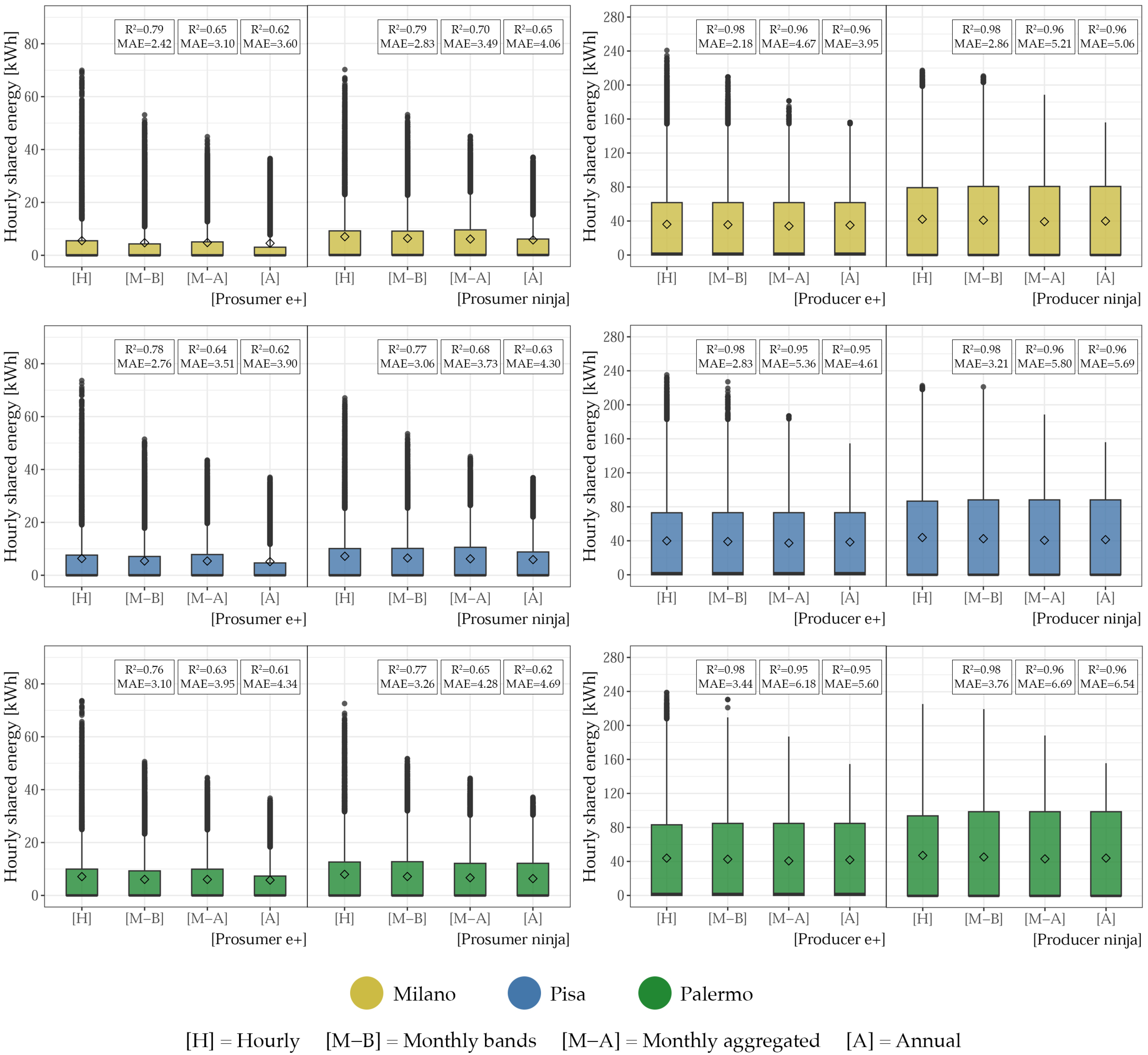
Figure 7 depicts the distribution of hourly shared energy during the first year of operation of the analysed configurations. For each case, the results are related to the four scenarios of simulations, which are obtained from the four different hourly input datasets employed. The first dataset, H, is the real one and is composed of the real hourly measured electrical consumption of the users. The other three scenarios are: the M–B scenario, obtained by estimating the hourly consumption of the users starting from monthly data divided according to Italian time bands; the M–A scenario, obtained through the estimation of hourly consumption data from monthly consumption; and the A scenario, obtained via estimation of the hourly consumption from annual consumption data. Specifically for the configuration characterized by only prosumers, simulations for scenarios M–B, M–A and A demonstrate the ability to approximate the realistic scenario H, achieving determination coefficients R2 ranging from 0.76 to 0.79 for M–B, 0.63 to 0.70 for M–A and 0.61 to 0.65 for A across three cities and using two weather files. Mean absolute errors (MAEs) are affected by numerous zero values but still average relatively high hourly amounts, ranging from 2.42 to 4.34 kWh.
In the cases with only one producer present, shared energy values are significantly higher. As a matter of fact, in the prosumers case, peak values of shared energy reach only 70 kWh because of user self-consumption patterns, while in the producer case, the peaks reach 240 kWh. This phenomenon results in MAEs ranging from 2.18 to 6.69, similar to the previous range. Nevertheless, when scaled to this higher range, the corresponding determination coefficients R2 are notably high, ranging from 0.95 to 0.98.
Average hourly shared energy values are generally similar and are influenced by periods of zero generation during nighttime hours when photovoltaic systems are inactive. However, maximum peaks vary among scenarios, as demonstrated in the consumption input example (Figure 3). Scenario H allows for an assessment of the actual distribution, with actual hourly consumption peaks reaching up to 2.4 kWh. The two monthly scenarios (M–B and M–A) reach maximum values of 0.55 kWh and 0.41 kWh, respectively, while scenario A evaluates peaks less favourably, not exceeding 0.3 kWh.
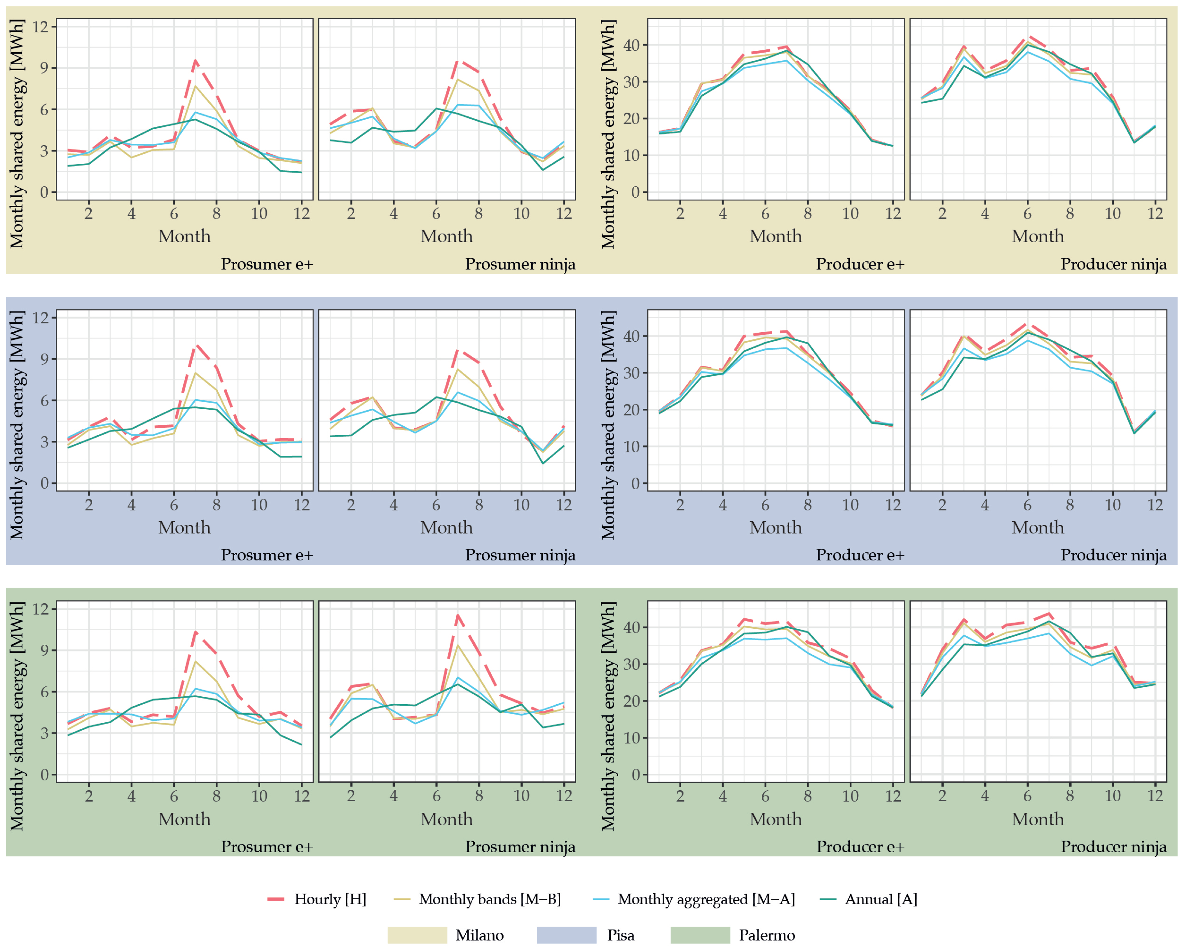
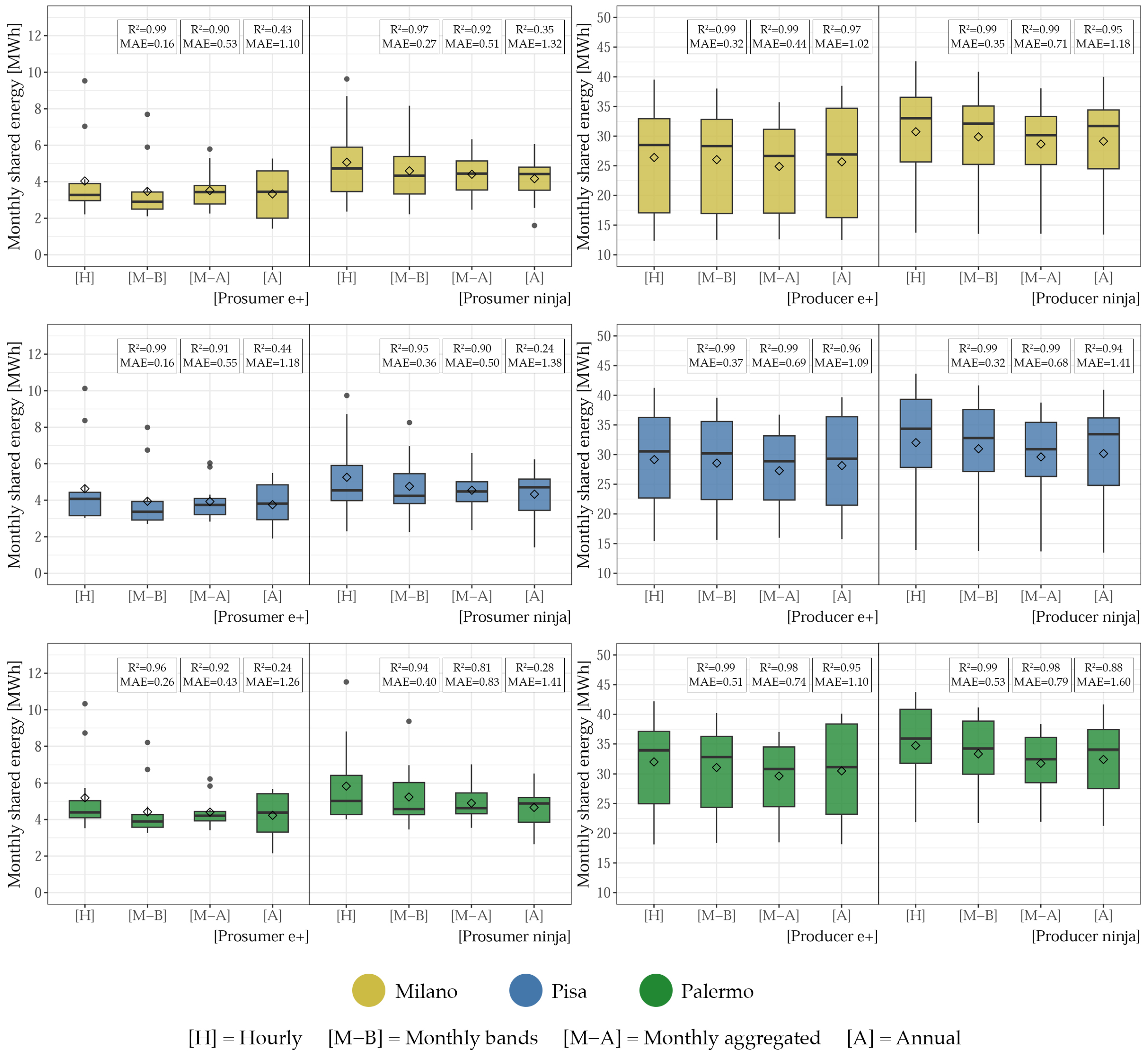
To investigate the impact of the data aggregation process on monthly outcomes, we grouped the hourly results in order to obtain monthly values of the results. Then, we plotted the trends of monthly shared energy for each month of the first year of operation of the studied configurations (Figure 8). Moreover, we analysed the distributions of these monthly values using boxplots, as shown in Figure 9. Aggregating the values of hourly shared energy into a single monthly value has smoothed out the differences that could be observed on an hourly basis, which is particularly evident in monthly cases (M–B) and (M–A), where R2 values consistently exceed 0.9. However, the annual case performs poorly at predicting monthly aggregates, with R2 dropping as low as 0.24 for prosumers and MAEs ranging around 1.3/1.4 MWh, with values averaging around 5 MWh (26/28% incidence). Coherent with the hourly distribution analysis described in the previous paragraph, the broader scale of results for the producer-only scenario tends to mask these discrepancies, showing R2 values greater than 0.9 even for the annual case (A).
The economic results presented in this paragraph have been calculated on an annual basis for 20 years of operation of the REC in all the considered scenarios (according to Italian law, 20 years is the reference duration for Italian REC studies). For each case, the computation of the NCF took into account several factors: the initial investment necessary to install the PV power systems, the operation and maintenance cost required to ensure the optimal functioning of PV systems themselves, the income from the sale of energy to the grid, the savings due to the non-purchase of energy from the grid through physical self-consumption and the revenue generated by the incentives related to shared energy. The analysis of the income distribution among community members does not fall within the objectives of of this paper. Figure 10 and Figure 11 depict the net cash flows of all the simulated configurations across the various studied scenarios. Figure 10 is related to the producer-only configuration, while Figure 11 is related to the prosumers-only one. In both pictures, dashed curves are used to indicate outcomes obtained using Renewables.Ninja to estimate PV production, while continuous curves relate to results gained by adopting EnergyPlus. In contrast, the colours are indicative of the four categories of consumption data aggregation.

4. Discussion

The investigation of the results highlighted three key concepts: the implications related to the use of aggregated consumption data in REC analysis, the influence of dealing with various geographical locations and of exploiting different weather files to evaluate PV energy production, and the findings’ practical impact. These concepts are the subject of a detailed discussion in the following subsections.

4.1. Implications of the Consumption Aggregations

For this study, real hourly measured consumption data have been grouped into three scenarios with different levels of aggregation in order to replicate common situations that frequently happen when dealing with feasibility studies for a REC under development. These scenarios served as inputs for the case study simulations and allowed us to observe actual variations in the outcomes obtained by the analysis of a REC. The calculation of shared energy involved the simultaneous consideration of several factors: photovoltaic energy production, prosumers’ self-consumption and the subsequent grid injection of surplus energy to fulfil the consumption needs of other members within the REC. In this context, the flattening of consumption across different scenarios, illustrated by an exemplary user’s profile in Figure 3, results in the loss of specific information and in the creation of increasingly unrealistic scenarios. In reality, designers may find themselves constrained to these scenarios due to limited detailed data availability. Without hourly data, certain consumption peaks cannot be accurately addressed, leading to a simplified analysis that does not fully capture the true dynamics of production–consumption alignment.
The random nature of different profiles is evident in the monthly trends shown in Figure 8. The general trend of the curves shown in this figure illustrates that the monthly bands case (M–B) closely approximates the pattern of the hourly case (H) because the partitioning of monthly consumption data according to time bands helps to maintain at least some information pertaining to the users’ behaviour. In terms of the ability to follow the reference profile, the M–B case is followed by the monthly case (M–A). Finally, as expected, for each analysed scenario, the annual case (A) shows the trend that is least close to that of the reference case. This variability is further confirmed by the values of R2 observed for both the hourly and monthly distributions of shared energy values (Figure 7 and Figure 9, respectively).
Moving to an economic perspective, Figure 10 and Figure 11 show the NCFs related to all the considered scenarios. At first glance, it is clear that for both figures, the curves can be divided into two distinct groups, which separate dashed curves (Ninja) from continuous ones (EnergyPlus). Conversely, when focusing on each group of curves, no significant differences attributed to data aggregation can be detected. That means that as for the economic analysis, the main discrepancies among the cases arise from the choice of the tool adopted to estimate PV energy production and not from the use of consumption data with increasing levels of aggregation. As a matter of fact, the values of PBT, which are determined based on where the curve intersects the x-axis, remain consistent across different aggregation scenarios but vary by approximately 1 year depending on the meteorological data used in the energy production simulations. On the other hand, the NPV at the 20th year varies by approximately EUR 30–70k due to different aggregation levels, but it varies by around EUR 120–230k due to variations in energy production associated with different weather files. These consideration are valid both for the producer-only case and the prosumer-only one.
Another interesting consideration is related to the order in which the NCF curves are arranged. As expected, this order again shows that the monthly bands scenario is the closest to the reference case. Conversely, the annual profile (A) appears to better align with the hourly scenario compared to the monthly one (M–A). This phenomenon can be explained by examining Figure 8: as has already been said, M–B curves are the ones that follow the reference case more closely, followed by M–A curves and, at last, by the A ones. Nevertheless, the A curves present higher monthly average values for shared-energy with respect to the M–A curves, thus leading to the phenomenon in the analysis (this finding is coherent with previous ones in [17]).

4.2. Impact of Simulations across Different Cities and Using Different Weather Files

Regarding the use of different weather files, it is important to emphasize that different outcomes have been obtained for both the energy and economic results. Although the trends of the analysed curves remain consistent in both cases, the values of shared energy are higher when computed using Renewables.Ninja for the estimation of PV energy production then when it is computed using EnergyPlus. Consider that the total annual production estimated by the two tools differs by approximately 5 MWh. This discrepancy is reflected in the average monthly shared energy values, which can vary by up to 1 MWh. This fact also leads to varying economic results, with higher NPV values and lower PBT values in the first case, and vice versa. Consequently, the same REC analysed exploiting the use of one weather file instead of another may lead to the forecasting of worse or better performance. It is essential to note that it would be incorrect to assert that one weather file is better than the other, but understanding the potential range of variation is crucial.
The absolute values differ among the three cities due to their varying photovoltaic production levels, which are influenced by their respective latitudes (averaging 73 MWh of yearly PV production in Milan, 79 MWh in Pisa and 86 MWh in Palermo). This variation leads to different average monthly shared energy values within the communities across the scenarios. For instance, if we consider the results for the producer-only scenario computed using EnergyPlus, the average monthly shared energy is around 27 MWh in Milan, around 30 MWh in Pisa and around 33 MWh in Palermo. The differing amounts of energy shared within the REC in these three locations result in varying revenues from incentives tied to shared energy, as the incentive amount is proportional to the energy shared. Despite this, the correction to the premium rate (foreseen by Italian law to take into account the different levels of solar radiation in different geographical areas) slightly mitigates the discrepancies in the economic outcomes. Moreover, no significant statistical variations among the three locations are observed due to the different data aggregations. The R2 values do not vary by more than 0.05 across the hourly values for the three cities, and nearly all monthly values show similar stability except for case A, which starts from a single annual value and exhibits slightly more randomized patterns. A slight difference is also observed in the MAEs, with values ranging from 1 to 2 kWh in hourly shared results and 0.2 to 0.4 MWh in monthly shared results. Moving to the economic data, they follow a similar pattern, with negligible variations due to data aggregation across the three cities. In fact, considering the results for the producer-only scenario computed using EnergyPlus, the NPV at the end of the twentieth year is EUR 0.75M for Milano, EUR 0.85M for Pisa and EUR 0.95M for Palermo, with PBTs ranging from 4.5 years for Milan, 4 years for Pisa and 3.5 years for Palermo.
In practice, a designer would find themselves dealing each time with a specific emerging REC placed in a well-defined geographical area. Given the above considerations, it is important to highlight that there are no significant discrepancies due to the impact of using consumption data with increasing aggregation levels in different geographic locations. However, the designer must be aware of the potential range of variations of the results they will obtain depending on the selected weather file to be used for the simulations.

4.3. Practical Impacts

The MAE values are similar, but the R2 scores depend on the magnitude of the results. An MAE of 3–5 kWh has little impact at higher magnitudes, such as in the producer-only case (maximum hourly 240 kWh and average 40 kWh). However, it has a more significant impact at lower magnitudes, like the prosumer-only case (maximum hourly 70 kWh and average 8 kWh). The R2 scores reflect this trend: higher precision is achieved in scenarios with high energy sharing, such as when there are many producers, whereas lower precision is observed in scenarios with low energy sharing, like in prosumer cases, where there is more self-consumption. This indicates that the aggregation of data has a more noticeable effect in scenarios with lower energy sharing, highlighting the importance of considering the specific configuration of the REC.
For managing a renewable energy community (REC), conducting analyses on an hourly basis is essential due to the high level of detail required to optimize operations and make real-time adjustments. This granular approach ensures that energy sharing and consumption patterns are accurately captured and managed. However, for other purposes, such as annual economic forecasting, a lower level of detail may be sufficient. In these cases, the differences between hourly and aggregated data tend to be minimal, and a more simplified approach can still provide reliable forecasts. Annual analyses focus on broader trends and cumulative outcomes, where the finer nuances of hourly data become less critical. Therefore, while hourly analyses are crucial for day-to-day management and operational efficiency, aggregated data can adequately support long-term economic planning and forecasting.

4.4. Limitations

To investigate the impact of consumption data aggregation in REC analysis, certain initial assumptions were made. While the case study was selected to be as general as possible, aiming to draw conclusions applicable to most common Italian RECs, the analysis relied on historical annual consumption data without accounting for future scenarios such as climate change or fluctuating energy prices. These assumptions facilitate a comparison and analysis, but they also limit the objectivity of the absolute results (e.g., shared energy and NCF). While these limitations do not affect the conclusions regarding the impact of data aggregation, they do influence the specific results reported, which, however, were not the primary focus of this analysis.

5. Conclusions

A case study characterized by real consumption data from different kinds of users representative of a typical community in Tuscany (a region located in the centre of Italy) was provided in order to investigate the influence of various factors on the analysis.
The present paper dealt with the analysis of a case study of a REC that was realized by exploiting real hourly measured consumption data from different kinds of users. The case study was representative of a typical community in the centre of Italy. The work compared the outcomes of the simulation of the REC based on real hourly measured consumption data (H scenario) with those of three simulations of the same REC based on three different datasets of hourly consumption loads estimated with increasing aggregation levels. To perform the comparison, the results obtained from case H were assumed to be the reference ones. With the purpose of widening the investigation on the influence of the aggregation of consumption data to outcomes related to the simulation of a REC, various scenarios were considered. Two different configurations were analysed: one consisting of consumers and prosumers and another composed of consumers and a single producer. In addition, three different locations were studied: one placed in the north, one in the centre and one in the south of Italy. Finally, the effects of two different weather files for the estimation of PV energy production were examined. Nonetheless, this work revealed some interesting insight. As for the configuration type of the REC, the presence of a producer replacing the prosumers resulted in a greater amount of shared energy within the community due to the absence of self-consumption. This fact highlighted that the values of R2 improved when shared energy increases, suggesting that the impact of consumption data aggregation is more evident in scenarios characterized by low sharing. In terms of geographical positioning of the REC, energy outcomes showed discrepancies that were related to the different levels of solar radiation affecting different areas. These discrepancies influenced economic results as well. Nonetheless, no differences could be detected in terms of influence of consumption aggregation, which was the same in all the analysed locations. Hence, the impact of utilising hourly consumption data estimated from aggregated ones remained consistent despite the varying geographical positioning of the RECs. This observation is of practical use for a designer, who has to deal with different geographical sites each time. Finally, concerning the use of different weather files, no discrepancies in the impact of the use of aggregated consumption data were detected.

Future Developments

Future research should expand beyond the exclusive consideration of PV plants to include other types of renewable energy systems. Since various generation systems can exhibit significantly different behaviour in terms of hourly energy production, it would be valuable to investigate how aggregated consumption data impact RECs with diverse types of generation plants.
For instance, studying wind-powered communities, which can also generate energy during nighttime, could offer insights into energy sharing during those hours. Similarly, coastal communities could leverage wave energy, which offers nearly continuous power. Biomass plants in forested areas also present unique opportunities. It is important to note that all of these renewable energy systems have distinct patterns, not only compared to PV plants but also among themselves. Therefore, investigating RECs with multiple power sources could yield a deeper understanding of their dynamics and benefits.

Author Contributions

Conceptualization, V.C., R.R. and M.R.; methodology, V.C. and R.R.; software, V.C. and R.R.; validation, V.C. and R.R.; formal analysis, V.C. and R.R.; investigation, V.C. and R.R.; writing—original draft preparation, V.C. and R.R.; writing—review and editing, V.C., R.R. and M.R.; supervision, M.R.; project administration, M.R.; funding acquisition, M.R. All authors have read and agreed to the published version of the manuscript.

Funding

This research was funded by the National Recovery and Resilience Plan (NRRP), Mission 4, Component 2, Investment 1.3—Call for tender No. 1561 of 11.10.2022 of Ministero dell’Università e della Ricerca (MUR) and was funded by the European Union—NextGenerationEU, Project Code PE0000021, Project Title “Network 4 Energy Sustainable Transition—NEST”.

Data Availability Statement

Electrical consumption data used in this work are not readily available because the owners shared them with the authors under a non-disclosure agreement.

Conflicts of Interest

The authors declare no conflicts of interest.

Abbreviations

The following abbreviations are used in this manuscript:
MESMulti-Energy System
NCFNet Cash Flow
NPVNet Present Value
PBTPay-Back Time
PVPhotovoltaic
RECRenewable Energy Community
TMYTypical Meteorological Year

Appendix A

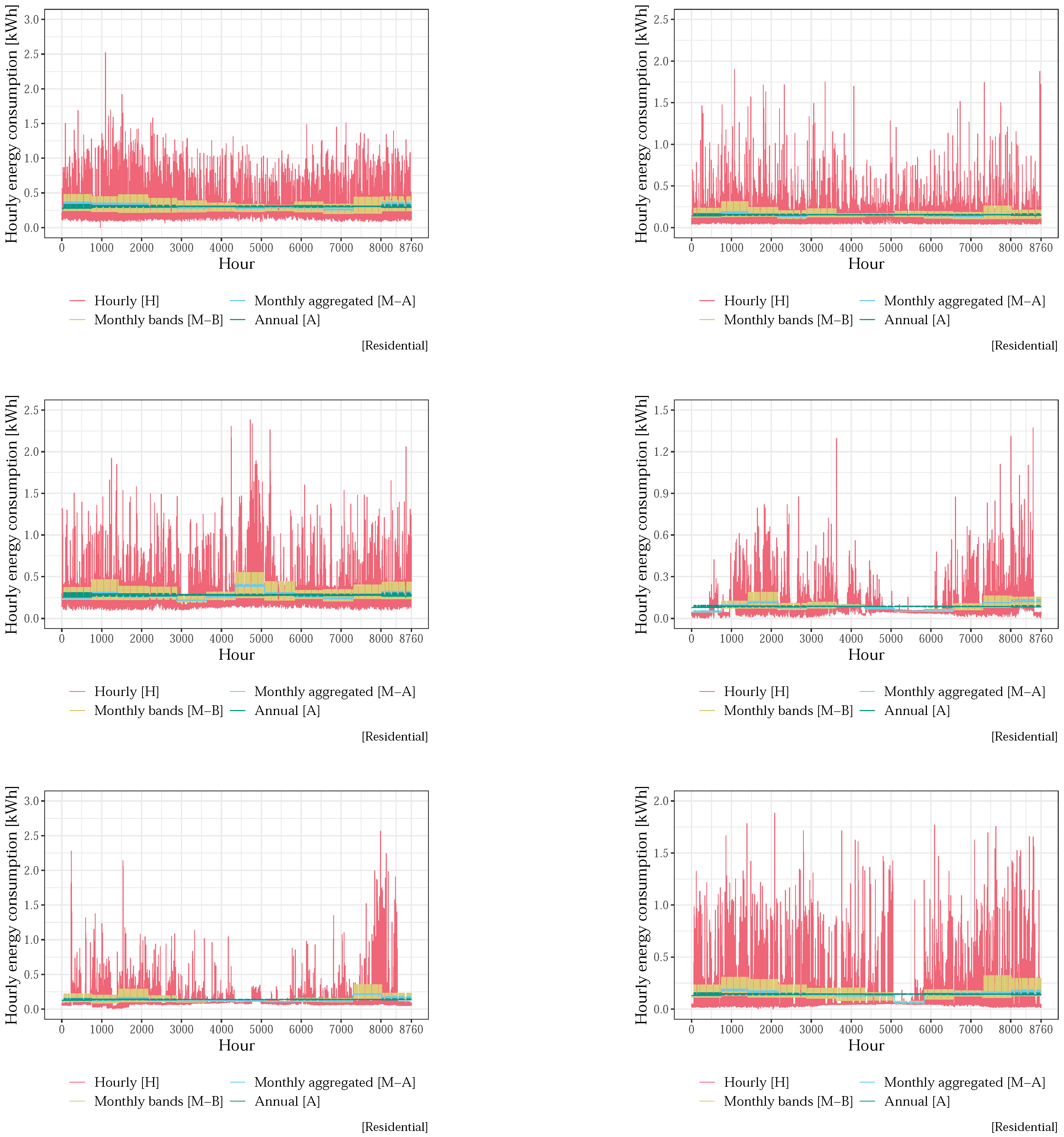
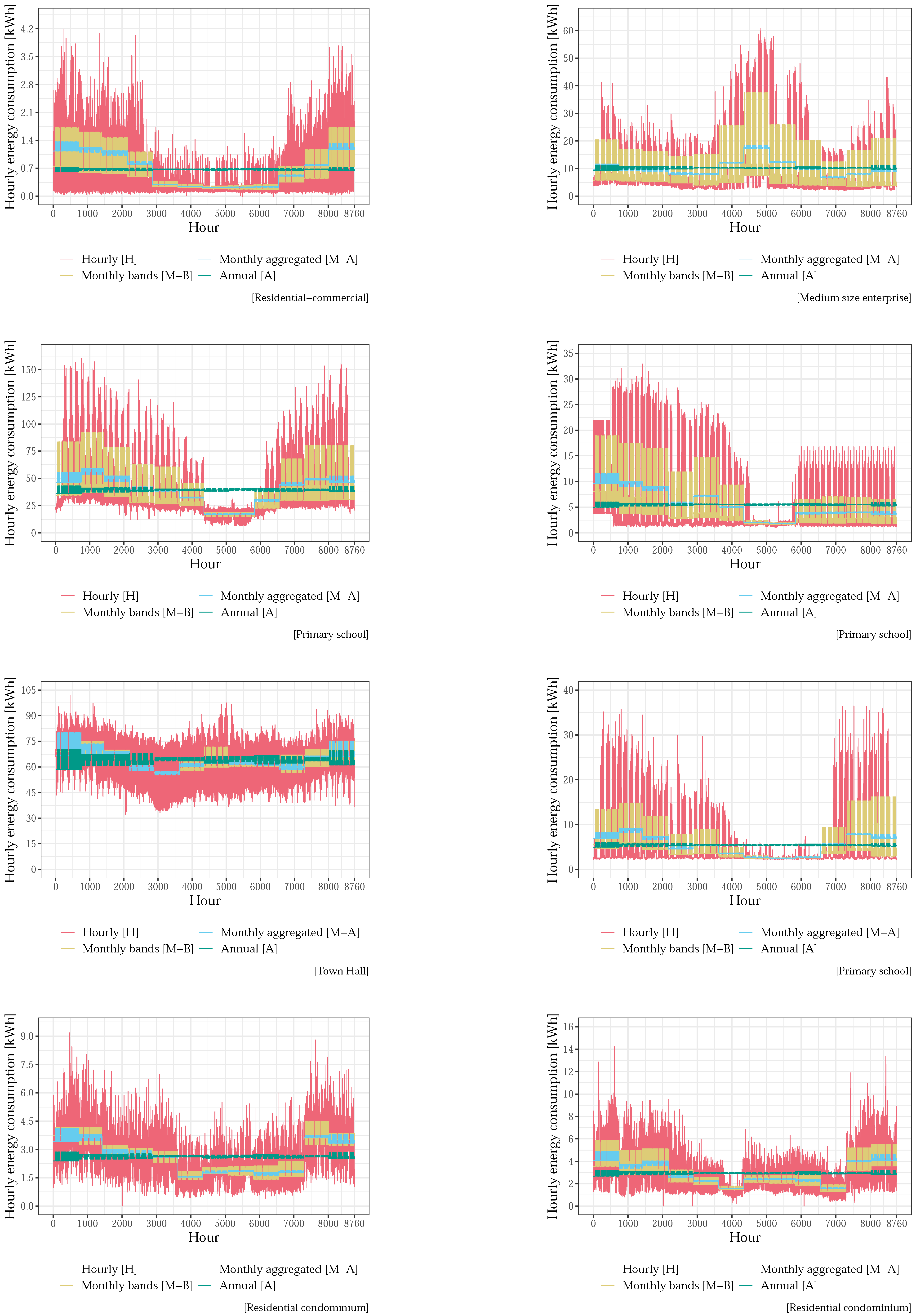
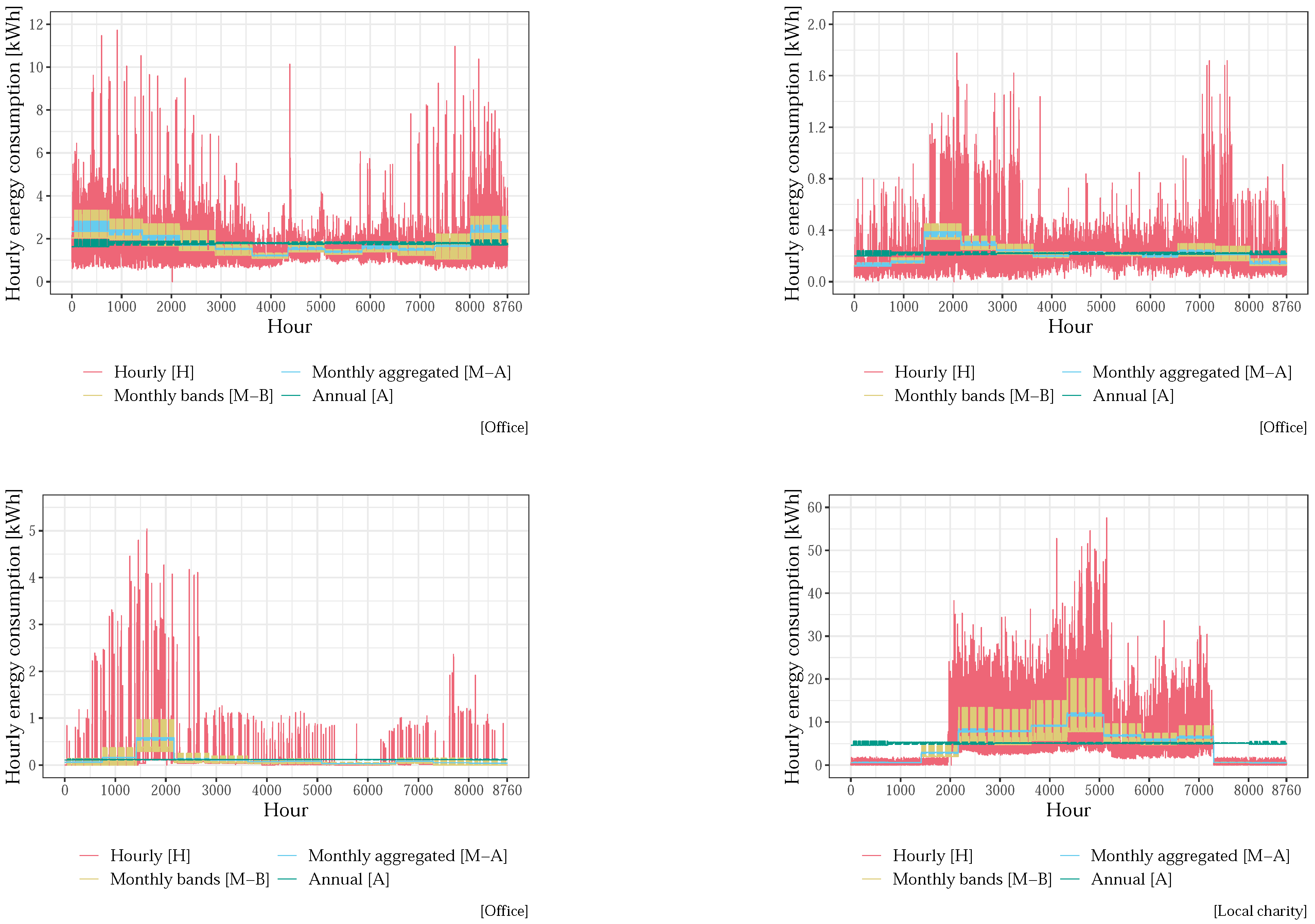
This appendix shows the consumption data for all twenty users considered. Each graph is related to a single user and illustrates the real hourly measured consumption and the three corresponding estimated hourly datasets obtained from the three increasing aggregation levels: monthly data divided by time bands, monthly data and annual data.
Figure A1. Hourly consumption of all users belonging to the REC over an entire year (8760 h). The presented data refer to: real hourly measured consumption (H), estimated hourly consumption from monthly data divided by time bands (M–B), estimated hourly consumption from monthly aggregated data (M–A) and estimated hourly consumption from annual aggregated data (A).
Energies 17 04647 g0a1aEnergies 17 04647 g0a1bEnergies 17 04647 g0a1c

References

  1. European Commission: Joint Research Centre; Uihlein, A.; Caramizaru, A. Energy Communities—An Overview of Energy and Social Innovation; Publications Office: Luxembourg, 2020. [Google Scholar]
  2. Green Power Communities List. 2024. Available online: https://www.epa.gov/greenpower/green-power-communities-list (accessed on 1 March 2024).
  3. Community Energy Map. 2023. Available online: https://cpagency.org.au/resources-2/map/ (accessed on 15 February 2024).
  4. Jadidbonab, M.; Mohammadi-Ivatloo, B.; Marzband, M.; Siano, P. Short-Term Self-Scheduling of Virtual Energy Hub Plant within Thermal Energy Market. IEEE Trans. Ind. Electron. 2021, 68, 3124–3136. [Google Scholar] [CrossRef]
  5. Zhang, N.; Sun, Q.; Yang, L.; Li, Y. Event-Triggered Distributed Hybrid Control Scheme for the Integrated Energy System. IEEE Trans. Ind. Inform. 2022, 18, 835–846. [Google Scholar] [CrossRef]
  6. Xu, D.; Zhou, B.; Wu, Q.; Chung, C.Y.; Li, C.; Huang, S.; Chen, S. Integrated Modelling and Enhanced Utilization of Power-to-Ammonia for High Renewable Penetrated Multi-Energy Systems. IEEE Trans. Power Syst. 2020, 35, 4769–4780. [Google Scholar] [CrossRef]
  7. Yang, L.; Li, X.; Sun, M.; Sun, C. Hybrid Policy-Based Reinforcement Learning of Adaptive Energy Management for the Energy Transmission-Constrained Island Group. IEEE Trans. Ind. Inform. 2023, 19, 10751–10762. [Google Scholar] [CrossRef]
  8. Barabino, E.; Fioriti, D.; Guerrazzi, E.; Mariuzzo, I.; Poli, D.; Raugi, M.; Razaei, E.; Schito, E.; Thomopulos, D. Energy Communities: A review on trends, energy system modelling, business models, and optimisation objectives. Sustain. Energy, Grids Netw. 2023, 36, 101187. [Google Scholar] [CrossRef]
  9. Sweeney, C.; Bessa, R.J.; Browell, J.; Pinson, P. The future of forecasting for renewable energy. WIREs Energy Environ. 2020, 9, e365. [Google Scholar] [CrossRef]
  10. Antonanzas, J.; Osorio, N.; Escobar, R.; Urraca, R.; de Pison, F.M.; Antonanzas-Torres, F. Review of photovoltaic power forecasting. Sol. Energy 2016, 136, 78–111. [Google Scholar] [CrossRef]
  11. Zheng, J.; Du, J.; Wang, B.; Klemeš, J.J.; Liao, Q.; Liang, Y. A hybrid framework for forecasting power generation of multiple renewable energy sources. Renew. Sustain. Energy Rev. 2023, 172, 113046. [Google Scholar] [CrossRef]
  12. Chen, S.; Yang, W.; Yoshino, H.; Levine, M.D.; Newhouse, K.; Hinge, A. Definition of occupant behavior in residential buildings and its application to behavior analysis in case studies. Energy Build. 2015, 104, 1–13. [Google Scholar] [CrossRef]
  13. Baglietto, G.; Massucco, S.; Silvestro, F.; Vinci, A.; Conte, F. A Non-Intrusive Load Disaggregation Tool based on Smart Meter Data for Residential Buildings. In Proceedings of the 2023 IEEE International Conference on Environment and Electrical Engineering and 2023 IEEE Industrial and Commercial Power Systems Europe (EEEIC / I&CPS Europe), Madrid, Spain, 6–9 June 2023; pp. 1–6. [Google Scholar] [CrossRef]
  14. Liu, J. Cluster Analysis of Electricity Consumption Characteristics and Electricity Consumption Behavior of Typical Industry Users. In Proceedings of the 2023 5th Asia Energy and Electrical Engineering Symposium (AEEES), Chengdu, China, 23–26 March 2023; pp. 1389–1395. [Google Scholar] [CrossRef]
  15. Chuang, M.; Yikuai, W.; Junda, Z.; Ke, C.; Feixiang, G.; Tao, C.; Songsong, C. Research on user electricity consumption behavior and energy consumption modeling in big data environment. In Proceedings of the 2021 IEEE 2nd International Conference on Big Data, Artificial Intelligence and Internet of Things Engineering (ICBAIE), Nanchang, China, 26–28 March 2021; pp. 220–224. [Google Scholar] [CrossRef]
  16. Lamagna, M.; Nastasi, B.; Groppi, D.; Nezhad, M.M.; Garcia, D.A. Hourly energy profile determination technique from monthly energy bills. Build. Simul. 2020, 13, 1235–1248. [Google Scholar] [CrossRef]
  17. Consolo, V.; Rugani, R.; Mura, E.; Raugi, M. Impact of power consumption at various aggregation levels in REC analysis: A real case study perspective. In Proceedings of the 2024 IEEE International Conference on Environment and Electrical Engineering (EEEIC), Roma, Italy, 17–20 June 2024. in press. [Google Scholar]
  18. Autorità di Regolazione per Energia Reti e Ambiente (ARERA), Rome, Italy. Proposte in Materia di Definizione delle Fasce Orarie per l’Anno 2007 e Successivi, atto n.19/06, Documento per la Consulatazione. 2006. Available online: https://www.arera.it/fileadmin/allegati/docs/06/dc_060703.pdf (accessed on 2 February 2024).
  19. Autorità di Regolazione per Energia Reti e Ambiente (ARERA), Rome, Italy. Aggiornamento Delle Fasce Orarie Con Decorezzenza 1 Gennaio 2007 Annex A. Delibera n.181/06. 2007. Available online: https://www.arera.it/atti-e-provvedimenti/dettaglio/06/181-06 (accessed on 2 February 2024).
  20. Pfenninger, S.; Staffell, I. Long-term patterns of European PV output using 30 years of validated hourly reanalysis and satellite data. Energy 2016, 114, 1251–1265. [Google Scholar] [CrossRef]
  21. Bellekom, S.; Arentsen, M.; van Gorkum, K. Prosumption and the distribution and supply of electricity. Energy Sustain. Soc. 2016, 6, 22. [Google Scholar] [CrossRef]
  22. Heinisch, V.; Odenberger, M.; Göransson, L.; Johnsson, F. Organizing prosumers into electricity trading communities: Costs to attain electricity transfer limitations and self-sufficiency goals. Int. J. Energy Res. 2019, 43, 7021–7039. [Google Scholar] [CrossRef]
  23. Gržanić, M.; Capuder, T.; Zhang, N.; Huang, W. Prosumers as active market participants: A systematic review of evolution of opportunities, models and challenges. Renew. Sustain. Energy Rev. 2022, 154, 111859. [Google Scholar] [CrossRef]
  24. IRENA. Renewable Power Generation Costs in 2022; International Renewable Energy Agency: Masdar, Abu Dhabi, 2023; Available online: https://www.irena.org/-/media/Files/IRENA/Agency/Publication/2023/Aug/IRENA_Renewable_power_generation_costs_in_2022.pdf (accessed on 2 February 2024).
  25. Rienecker, M.M.; Suarez, M.J.; Gelaro, R.; Todling, R.; Bacmeister, J.; Liu, E.; Bosilovich, M.G.; Schubert, S.D.; Takacs, L.; Kim, G.K.; et al. MERRA: NASA’s modern-era retrospective analysis for research and applications. J. Clim. 2011, 24, 3624–3648. [Google Scholar] [CrossRef]
  26. Autorità di Regolazione per Energia Reti e Ambiente (ARERA), Rome, I. Allegato A alla deliberazione 727/2022/R/eel. Testo Integrato Delle Disposizioni Dell’autorità Di Regolazione Per Energia Reti E Ambiente Per La Regolazione Dell’autoconsumo Diffuso (Testo Integrato Autoconsumo Diffuso - TIAD) 2022-12-27. Available online: https://www.arera.it/fileadmin/allegati/docs/22/727-22.pdf (accessed on 31 January 2024).
  27. Ministero Dell’Ambiente e Della Sicurezza Energetica. Decreto CER. 24 January 2024. Available online: https://www.jtf.gov.it/wp-content/uploads/2024/01/Decreto-CER.pdf (accessed on 31 January 2024).
  28. Gestore Mercati Energetici (GME). Esiti MGP. Available online: https://gme.mercatoelettrico.org/it-it/Home/Esiti/Elettricita/MGP/Esiti/PUN (accessed on 10 May 2024).
  29. Moncecchi, M.; Meneghello, S.; Merlo, M. A Game Theoretic Approach for Energy Sharing in the Italian Renewable Energy Communities. Appl. Sci. 2020, 10, 8166. [Google Scholar] [CrossRef]
  30. Condizioni Economiche per i Clienti del Mercato Tutelato. 2024. Available online: https://www.arera.it/area-operatori/prezzi-e-tariffe/condizioni-economiche-per-i-clienti-del-mercato-tutelato (accessed on 2 February 2024).
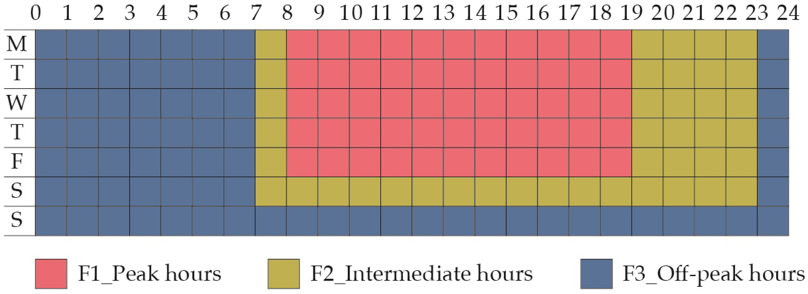
Figure 1. Hourly band matrix used to calculate energy consumption in Italy. The hours in F1 represent peak hours, where higher energy usage results in elevated prices. F2 denotes the intermediate band, while F3 signifies the period of lower consumption and, consequently, lower prices. Public holidays are treated as Sundays. Days of the week are listed in the rows from Monday (M) to Sunday (S), while the columns indicate the hours of the day.
Energies 17 04647 g001
Figure 2. Methodology flowchart. Starting from the left: the input hourly data for the task, their aggregation to create the four initial scenarios, followed by the data processing phase where the aggregated data were also reverted to hourly data. These processed data were then input into the MATLAB R2023b code, which managed shared energy within the REC on an hourly basis.
Energies 17 04647 g002
Figure 3. Hourly consumption of a user belonging to the REC over an entire year (8760 h). The presented data refer to: real hourly measured consumption (H), estimated hourly consumption from monthly data divided by time bands (M–B),estimated hourly consumption from monthly aggregated data (M–A) and estimated hourly consumption from annual aggregated data (A).
Energies 17 04647 g003
Figure 4. Annual evolution of daily temperatures of Milano, Pisa, and Palermo. The solid lines represent the daily averages, while the opaque coloured areas indicate the hourly minimum and maximum values observed throughout the day. The results are presented for both the Meteonorm and MERRA-2 weather files.
Energies 17 04647 g004
Figure 5. Annual evolution of global radiation for Milano, Pisa and Palermo. The solid lines represent the daily averages, while the opaque coloured areas indicate the hourly minimum and maximum values observed throughout the day. The results are presented for both the Meteonorm and MERRA-2 weather files.
Energies 17 04647 g005
Figure 6. Estimated price of energy P E .
Energies 17 04647 g006
Figure 7. Hourly shared energy distribution within the REC during the first year of operation. Results are shown for the three cities of Milano, Pisa and Palermo for the two different configurations with either prosumers-only or a producer-only and for the two tools adopted for the estimation of the PV energy production: EnergyPlus (e+) and Renewables.Ninja (ninja). Values are reported for each hour. R2 and MAE values are specified for the three cases (M–B, M–A and A) in comparison to the reference case (H).
Energies 17 04647 g007
Figure 8. Monthly shared energy within the REC during the first year. Values are reported for each month in the four studied scenarios for the three cities of Milano, Pisa and Palermo for the two different configurations of either prosumer-only or producer-only for the two tools adopted for the estimation of the PV energy production: EnergyPlus (e+) and Renewables.Ninja (ninja).
Energies 17 04647 g008
Figure 9. Monthly shared energy distribution within the REC during the first year of operation for the three cities of Milano, Pisa and Palermo for the two different configurations of either prosumer-only or producer-only for the two tools adopted for the estimation of the PV energy production: EnergyPlus (e+) and Renewables.Ninja (ninja). Values reported for each hour. R2 and MAE are specified for the three cases (M–B, M–A, and A) in comparison to the reference case (H).
Energies 17 04647 g009
Figure 10. NCF curves with the annual NPV values for the REC with only one producer. Values are reported for each year in the four studied scenarios for the three cities of Milano, Pisa and Palermo for the two tools adopted for the estimation of the PV energy production: EnergyPlus and Renewables.Ninja.
Energies 17 04647 g010
Figure 11. NCF curves with the annual NPV values for the REC with only prosumers. Values are reported for each year in the four studied scenarios for the three cities of Milano, Pisa and Palermo for the two tools adopted for the estimation of the PV energy production: EnergyPlus and Renewables.Ninja.
Energies 17 04647 g011
Table 1. Symbols.
Table 1. Symbols.
SymbolMeaningType
AAnnual consumption data of a single userScalar
r m Ratio between the number of days of the month m and the number of days of the yearScalar
r Vector containing all the ratios r m Vector
l m Monthly consumption vectorVector
r b , m Ratio between the number of hours of each time band and the number of hours of the month itselfScalar
R b m Matrix containing all the ratios r b , m Matrix
L m b Monthly consumption divided by time bandsMatrix
l m b Monthly consumption divided by time bandsVector
H b Matrix defining whether each hour of the year belongs to a specific time band or notMatrix
l h Estimated hourly consumptionVector
Table 2. Economic parameters.
SymbolParameterValue
C u , P V Unit cost of PV systems1300 EUR/kWp
C y , m Annual cost of maintenance (as a % of C u , P V )2%
dDiscount rate3.5%
P U N a v Average electricity price180 EUR/MWh
Disclaimer/Publisher’s Note: The statements, opinions and data contained in all publications are solely those of the individual author(s) and contributor(s) and not of MDPI and/or the editor(s). MDPI and/or the editor(s) disclaim responsibility for any injury to people or property resulting from any ideas, methods, instructions or products referred to in the content.