Article

An Integrated CEEMDAN to Optimize Deep Long Short-Term Memory Model for Wind Speed Forecasting

1
School of Computer Engineering, Chongqing College of Humanities, Science & Technology, Chongqing 401524, China
2
Research Center for Big Data and Network Information Security Engineering Technology, Chongqing College of Humanities, Science & Technology, Chongqing 401524, China
3
School of Civil Engineering, Chongqing University, Chongqing 400045, China
*
Author to whom correspondence should be addressed.
Energies 2024, 17(18), 4615; https://doi.org/10.3390/en17184615
Submission received: 8 August 2024 / Revised: 3 September 2024 / Accepted: 10 September 2024 / Published: 14 September 2024
(This article belongs to the Special Issue Advances in Wind and Solar Farm Forecasting—3rd Edition)

Abstract

:
Accurate wind speed forecasting is crucial for the efficient operation of renewable energy platforms, such as wind turbines, as it facilitates more effective management of power output and maintains grid reliability and stability. However, the inherent variability and intermittency of wind speed present significant challenges for achieving precise forecasts. To address these challenges, this study proposes a novel method based on Complete Ensemble Empirical Mode Decomposition with Adaptive Noise (CEEMDAN) and a deep learning-based Long Short-Term Memory (LSTM) network for wind speed forecasting. In the proposed method, CEEMDAN is utilized to decompose the original wind speed signal into different modes to capture the multiscale temporal properties and patterns of wind speeds. Subsequently, LSTM is employed to predict each subseries derived from the CEEMDAN process. These individual subseries predictions are then combined to generate the overall final forecast. The proposed method is validated using real-world wind speed data from Austria and Almeria. Experimental results indicate that the proposed method achieves minimal mean absolute percentage errors of 0.3285 and 0.1455, outperforming other popular models across multiple performance criteria.

1. Introduction

Renewable energy sources [1,2] can help protect the natural environment by avoiding fossil fuel emissions and allowing for more efficient utilization of available land and space resources. Wind power, as a cheap and clean energy source, harnesses the natural power of wind to generate electricity [3,4]. It is abundant, inexhaustible, and emits no greenhouse gases during operation, making it an ideal solution in our quest for sustainability. Evidence suggests that wind energy is expected to account for 22% of global electricity generation by 2030 [5]. Wind power is highly dependent on wind speed. Since wind speed is unpredictable and random, integrating wind power into the grid has considerable difficulties in system operation and dispatch [6]. Thus, it is critical to have accurate wind speed forecasting methods.
Researchers have developed various wind speed forecasting techniques to improve forecast accuracy. These methods can be divided into two categories: statistical analysis and artificial intelligence (AI) methods. Statistical analysis utilizes historical wind speed data to forecast future data. These methods include autoregressive integrated moving average (ARIMA) models [6], autoregressive (AR) [7], and Kalman filtering [8]. For instance, Yunus et al. [9] present a novel wind speed forecasting method using a modified ARIMA model. The model separates high- and low-frequency components and applies additional techniques to capture the time correlation and distribution. Location-specific models provide a new technique for wind speed prediction using only average speeds, advancing wind forecasting methods. Xie et al. [10] propose a probabilistic short-term wind power prediction method. An infinite Markov switching autoregressive model captures the dynamics of the wind power process and quantifies the forecast uncertainty. The method provides accurate and reliable short-term wind power probabilistic forecasts to support the real-time risk management of smart grids. Wang et al. [11] propose a hesitant fuzzy time series forecasting model for wind speed prediction. The model extracts effective features using advanced decomposition methods and determines the weights of different intervals by multi-objective optimization algorithms. Experiments show that the proposed model can improve forecasting accuracy and efficiency compared to other models. Traditional statistical analysis, which is fundamentally based on linear assumptions, struggles to accurately capture the intricate nonlinear relationships and dynamics of a time series. Moreover, these methods fail to account for the complex behaviors and feedback mechanisms inherent to nonlinear systems.
Artificial intelligence models have developed rapidly recently for wind speed prediction due to their strong nonlinear fitting ability. Popular AI algorithms include Long Short-Term Memory Neural Networks (LSTM) [12,13,14], Support Vector Machines (SVM) [15,16], and other deep learning architectures [17]. For instance, Zameer et al. [18] propose a genetic programming-based neural network ensemble regression for short-term wind power forecasting. The prediction becomes more intelligent and robust by allowing genetic programming to semi-stochastically combine multiple neural networks to construct a collective decision space. Experiments on five wind farms in Europe show that this method achieves higher accuracy than others. Jiang et al. [19] propose a combined wind speed forecasting system that includes sub-model selection, point forecasting based on multi-objective optimization, interval forecasting by distribution fitting, etc. The combined system integrates the advantages of various sub-models and can effectively generate accurate point forecasts and reliable interval forecasts of wind speed. Shahid et al. [20] propose a novel LSTM method based on recurrent neural networks with wavelet kernels for wind power prediction. The method combines the advantages of deep learning and wavelet transformations to capture the temporal and nonlinear characteristics of wind power data. Liu et al. [21] propose a novel deep learning model for wind speed forecasting to address fluctuations. It uses data preprocessing, ensemble learning, and multi-error correction. The experimental results demonstrate superior performance compared to other models in terms of stability and accuracy, especially for multi-step forecasting.
The intrinsic variability and intermittency of wind speed manifest as randomness and fluctuation in the wind speed data. These characteristics make it difficult to achieve accurate wind speed predictions through the use of a single forecasting technique. Therefore, several decomposition-based hybrid methods have been employed in the field of wind speed forecasting, such as Empirical Mode Decomposition [22], Ensemble Empirical Mode Decomposition (EEMD) [23,24], and Complementary EEMD (CEEMD) [25,26]. For instance, Qu et al. [27] propose an ensemble approach optimized by a novel multi-objective algorithm. It incorporates data preprocessing, assesses model accuracy and stability via bias-variance optimization, and searches for optimal weights using a hybrid flower pollination and bat algorithm. Experiments on 12 wind speed datasets show that the ensemble model provides superior precision and stability over existing models. Jaseena et al. [28] propose a framework combining data decomposition techniques like Wavelet Transform to denoise the signal and Bidirectional LSTM networks to separately forecast the decomposed low and high-frequency components. Experiments show that the proposed model outperforms other decomposition and deep learning models in terms of accuracy and stability for wind speed prediction.
Considering the analysis above, this study proposes a new modeling framework based on CEEMDAN-LSTM for wind speed forecasting. The framework aims to leverage the strengths of CEEMDAN and LSTM to achieve more accurate wind speed prediction. Specifically, CEEMDAN is first utilized to decompose the wind speed into a set of Intrinsic Mode Functions (IMFs) and a Residual (Res). The IMFs and Res are then used to construct the input features that feed into the subsequent LSTM network. The LSTM model can capture the sequential data’s temporal dependencies and nonlinear relationships. The final wind speed is obtained by reconstructing the prediction sequences. The method is validated on real-world wind speed data in Austria and Almeria, which shows better performance than other mainstream methods such as Long Short-Term Memory (LSTM), Gated Recurrent Unit (GRU), Deep Neural Network (DNN), Support Vector Regression (SVR), and Decision Tree Regression (DTR). The remainder of this study is as follows. Section 2 briefly introduces the framework of the proposed method. Section 3 describes the experimental data and evaluation indicators. The experimental results and analyses are presented in Section 4. Finally, Section 5 concludes the study and discusses potential directions for future research.

2. Methodology

The proposed CEEMDAN-LSTM model for wind speed forecasting in this study is illustrated in Figure 1. The CEEMDAN model is utilized to decompose wind speed sequences into IMFs to capture local multiscale time properties and Res components. For each IMF and the Res, prediction models are constructed using LSTM to learn long dependence in sequence prediction problems. The final step involves summing up all the predicted IMFs and Res, which can yield a reconstructed wind speed curve. The CEEMDAN-LSTM ensures a more accurate and reliable prediction by considering both the multiscale characteristics of wind speed and the powerful sequence learning ability of LSTM networks.

2.1. Complete Ensemble Empirical Mode Decomposition with Adaptive Noise

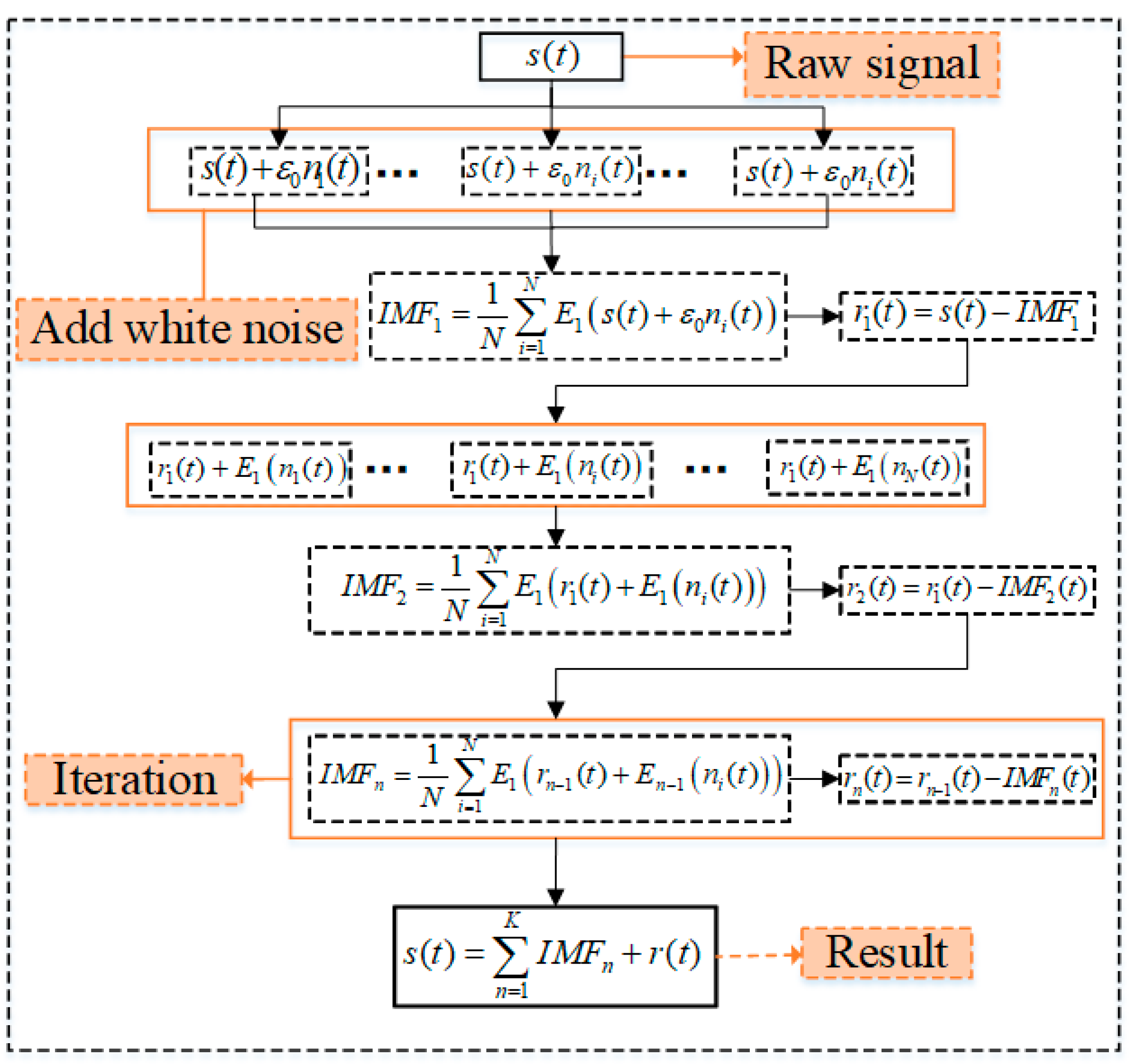
CEEMDAN introduces two improvement strategies: adaptive noise level and complete ensemble average. The adaptive noise level adjusts the noise intensity dynamically according to the signal’s local features to minimize noise interference on the signal while ensuring the orthogonality and completeness of the IMFs. A complete ensemble average is used to perform two ensemble averages for each IMF, one after adding different levels of white noise and the other after adjusting the adaptive noise level, to improve the accuracy and stability of signal decomposition. Thus, it is a powerful tool for analyzing nonlinear and non-stationary time series data, and is particularly useful in wind speed forecasting. By obtaining the IMFs through CEEMDAN, the pre-processed data becomes more suitable for input into the wind speed prediction model, as shown in Figure 2.
The algorithm steps of CEEMDAN are as follows:
(1)
White noise with zero mean and unit variance is superimposed on the original signal S(t) to create a new signal S′(t).
S i ( t ) = S ( t ) + v i ( t ) , i = 1 , 2 , , I
(2)
The signal S i ( t ) is decomposed into IMFs (IMF1, IMF2, …, IMFn) and a residue r(t) using EMD.
I M F ^ 1 = 1 I i = 1 I I M F 1 i
r 1 ( t ) = S ( t ) I M F ^ 1
(3)
Add white noise v i ( t ) into the residual signal r 1 ( t ) and conduct I experiments (I = 1, 2, …, I). In each experiment, use EMD to decompose r 1 i ( t ) = r 1 ( t ) + v i ( t ) into its first-order component I M F 1 i . The second CEEMDAN mode is described as:
I M F ^ 2 = 1 I i = 1 I I M F 1 i
r 2 ( t ) = S ( t ) I M F ^ 2
(4)
Reiterate the above decomposition process to extract IMF components that satisfy the criteria and their associated residuals. The process concludes when the residual becomes a monotonic function that can no longer be decomposed through EMD. The original signal S(t) can be reconstructed from the extracted IMF components.
S ( t ) = k = 1 K I M F k ^ + r k ( t )

2.2. Long Short-Term Memory Neural Network

Long Short-Term Memory (LSTM) neural networks are a type of recurrent neural network (RNN) that are well-suited for learning long-term dependencies in time series data [29]. The fundamental essence of LSTM lies in its utilization of the unit state and three gate structures: the input gate, forget gate, and output gate. These gate structures play a pivotal role in regulating the flow of information within the LSTM unit, effectively controlling the transmission of information throughout the network. By leveraging its distinctive information transmission path, LSTM effectively tackles the challenge of vanishing gradients that traditional RNNs often encounter [30,31]. The calculation formulas of the LSTM structure are as follows in Figure 3.
The forget gate of LSTM is responsible for determining the extent to which the previous state should be preserved. This forget gate can be mathematically described as follows:
f t = σ w f x x t + w f h H t 1 + b f
where σ   = ( 1 + e x ) 1 is sigmoid function and its value between 0 and 1. w f x and w f h represents weight parameters. b f is the bias.
The input gate in LSTM plays a crucial role in determining the new information that should be incorporated into the current cell state. This gate is responsible for selectively adding relevant information to the LSTM unit. Its mathematical representation can be seen in the following equation.
  i t = σ w i x x t + w i h H t 1 + b i
  c i t = tanh w c x x t + w c h H t 1 + b c  
U t = f t U t 1 + i t c i t
where w , w f h , w c x , w c h represent weight parameters, respectively. b i , b c are the bias of input gate. denotes element multiplication operation.
The output gate in LSTM is in charge of determining the specific information that needs to be outputted from the cell state. It selectively filters and controls the information flow to generate the relevant output, which can be described as follows:
o t = ReLU w o x x t + w o h H t 1 + b o
H t = o t tanh U t
where tanh = e x e x / e x + e x represents a hyperbolic tangent function. w o x and w o h are weight parameters. b o is the bias of output gate.
The LSTM cell employs the forget, input, and output gates to govern, updating its internal cell state and producing output predictions. These gates are crucial in controlling the information flow and manipulation within the LSTM cell, enabling it to make accurate predictions effectively.

2.3. Model Parameter Setting and Compared Models

Given that the prediction outcome can be influenced by various factors, such as the number of hidden layers and neurons, it becomes crucial to employ an optimization technique to enhance the performance of the CEEMDAN-LSTM model. In this regard, grid search, a robust and widely used model, is deployed to determine the optimal values for the neural parameters [32,33]. Using different combinations of hidden layer configurations and neuron counts, a grid search can obtain the most optimal parameters for the CEEMDAN-LSTM model, which yields the best prediction results. The search parameters, including Batch size, Learning rate, Drop regularization, and Neurons in the hidden layer, are in Table 1. Finally, after experimentation and analysis, the optimal parameter settings are as follows: the batch size is set to 32, the learning rate is 0.0001, the dropout regularization is 0.2, and there are 16 and 5 neurons in the hidden layer.
Table 2 shows the parameters and their potential value ranges used in the grid search for each comparative model. Notably, the parameter settings of DNN, LSTM, GRU, EMD-CNN, EMD-LSTM, and CEEMDAN-CNN (such as Batch size, Learning rate, and Dropout regularization) are consistent with the proposed CEEMDAN-LSTM model. This consistency ensures the fairness and reliability of the comparative experiments. As can be discerned from the Table 2, critical parameters for the LSTM, GRU, and EMD-LSTM models primarily include the number of neurons in their main layers and the number of neurons in the fully connected layers. For the DNN model, the focus is predominantly on the number of neurons in the fully connected layers. The DTR model parameters include the tree’s maximum depth (max depth), minimum number of samples required for node splitting (min samples split), and minimum number of samples required for leaf nodes (min samples leaf). The SVR model emphasizes the regularization parameter, the scale parameter gamma of the kernel function, and the type of kernel function (kernel). This detailed parameter setting offers an accurate reference for further exploring each model’s performance. For the EEMD-CNN and CEEMDAN-CNN models, the filter number of the convolution layer and the number of neurons in a fully connected layer are emphasized, which directly influence the models’ ability to capture and learn relevant features from the input data.

3. Experimental Data and Evaluation Indicators

In this study, two wind speed datasets from Austria and Almeria are selected for analysis. The statistical indicators of wind speed include the average wind speed, maximum wind speed, minimum wind speed, standard deviation, skewness, and kurtosis, which describe the essential characteristics and distribution of wind speed. Then, CEEMDAN decomposes the nonlinear and non-stationary wind speed signal into limited IMFs and Res, each representing a different frequency component, revealing the wind speed signal’s inherent structure and variation law.

3.1. Wind Speed Measurements in Austria

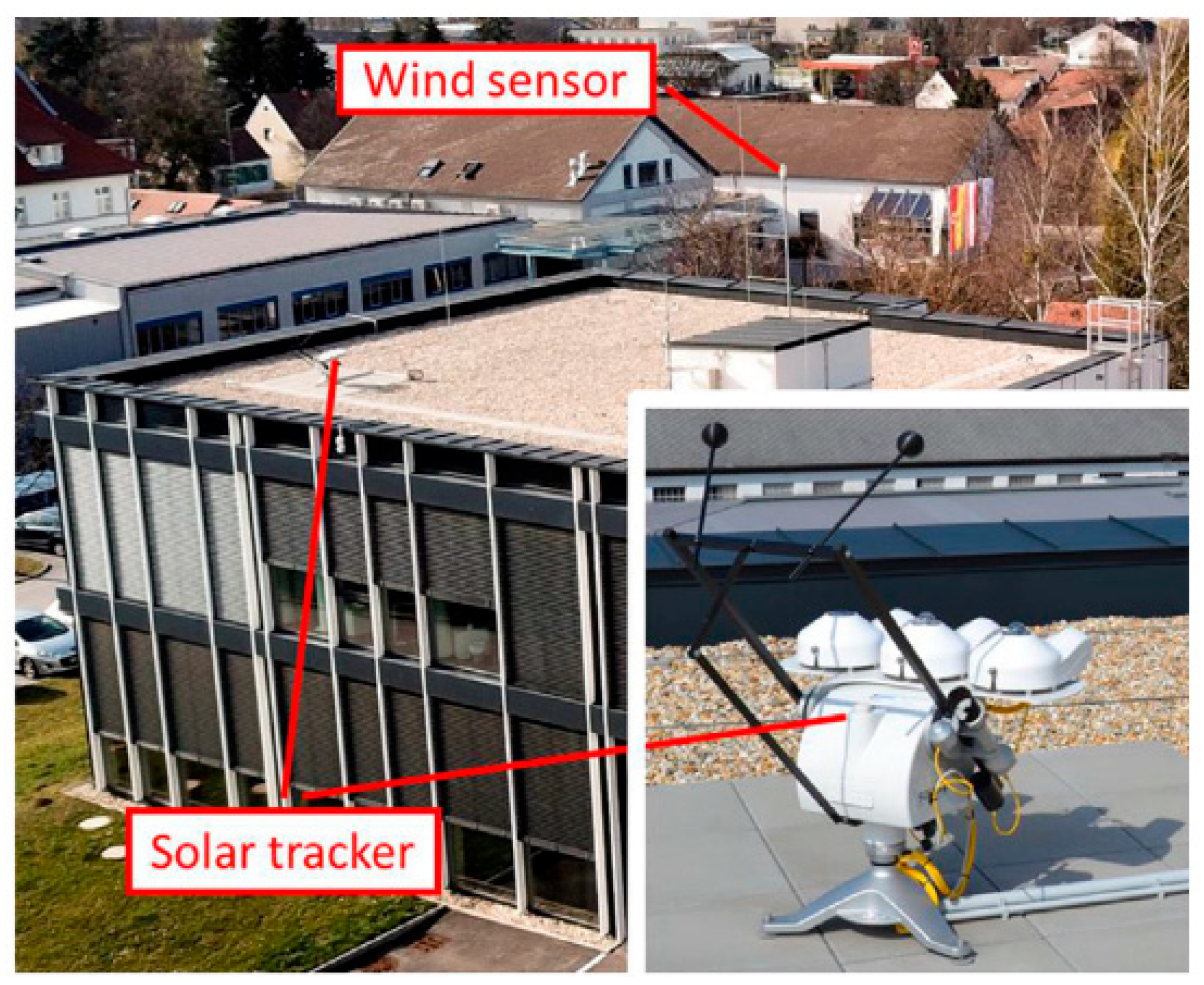
This dataset is gathered through the real-world operation of a hybrid photovoltaic thermal (PVT) solar collector on an experimental test setup with an average time interval of 5 s. The weather collection system utilizes pyranometers, NTC temperature sensors, and LUFFT wind sensors to record various weather parameters, such as ambient temperature, solar tracker path, wind speed, humidity, and wind direction, as shown in Figure 4. This dataset covers a period of 58 summer days, specifically from 11 July to 6 September, with a time step of 5 s [34].
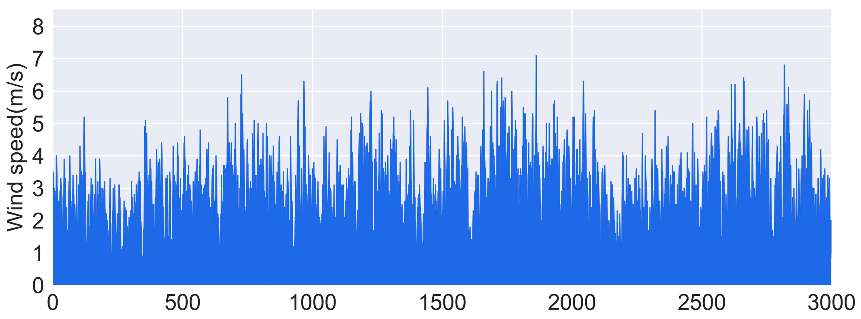
Figure 5 presents a subset of the wind speed data collected in Austria. Among the recorded values, the maximum wind speed is 7.10 m/s, while the minimum wind speed is 0.28 m/s. The average wind speed is calculated to be 1.1590 m/s. In addition, by analyzing the statistical properties of the dataset, the kurtosis value [35] is found to be 0.0090, suggesting a relatively normal distribution with moderate peakedness. Furthermore, the skewness value [36] is measured at 0.4399, indicating a slightly positively skewed distribution of wind speeds. These statistical measures offer valuable insights into the characteristics of the wind regime in Austria.
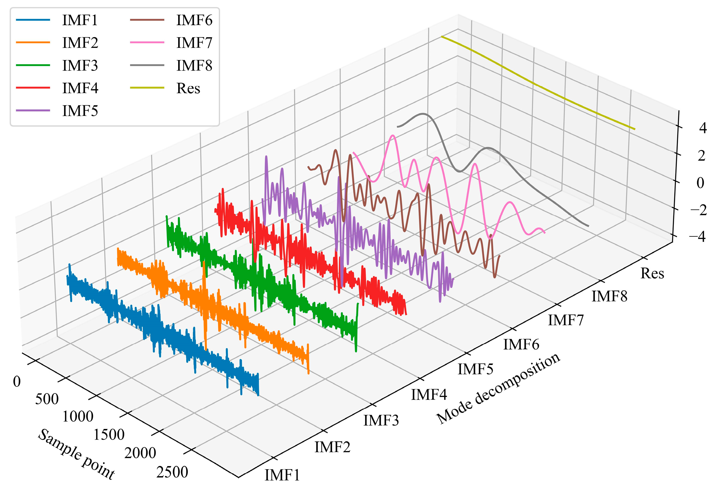
Mode decomposition algorithms have been demonstrated to mitigate the non-stationarity of time series and aid in noise filtration, thereby enhancing forecasting accuracy [37,38]. As a mode decomposition algorithm, CEEMDAN is an enhanced version of Empirical Mode Decomposition (EMD). It can adjust the Gaussian white noise to each IMF using the noise coefficient vector. In this way, it can effectively address several limitations of EMD and its other variants, such as mode mixing and high computation. In addition, it is essential to note that the sum of the IMFs and the residual acquired from CEEMDAN can fully rebuild the original series. According to Figure 6, the wind speed is decomposed into nine IMFs and a Res through the CEEMDAN model.
Table 3 displays various IMF components and the Res component. Among these, the frequencies of IMF1 to IMF8 progressively decline, surpassing that of the Res component. The Res component incrementally rises from a minimum of 2.15 to a maximum of 2.93, accurately portraying the fluctuating pattern of the wind speed time series. The average values of the IMFs are considerably lower than their respective standard deviations, indicating their continuous oscillations within the entire series. Regarding skewness, most IMFs have values near zero, suggesting a fairly symmetrical distribution around the mean. The exception is the Res, which exhibits substantial negative skewness (−1.0382), hinting at a potential left-leaning distribution. Kurtosis values offer additional insights into the distribution characteristics of each IMF. A mix of positive and negative kurtosis values across IMFs implies varying tail weights in the distribution, with some IMFs potentially showing more tail-heavy (leptokurtic) or tail-light (platykurtic) distributions.

3.2. Wind Speed Measurements in Almeria

In the highlands of Almeria city, Spain, Andalusia, wind speed data is collected from three meteorological stations: “Collado Yuste” (station 1), “Solana del Zapatero (station 2)”, and “Calar Alto (station 3)”. Each station has an anemometer to measure wind speed at regular intervals of 600 s (10 min) [39]. In this study, the wind speed data from the station 1 is specifically chosen for further analysis and prediction in Figure 7.
The raw wind speed dataset is presented in Figure 8, which shows the variation in wind speed over time. The dataset has a wide range of wind speed values, ranging from a minimum of 0.150 m/s to a maximum of 15.110 m/s. The mean wind speed is 4.511 m/s, indicating that the wind speed is generally moderate. However, the dataset exhibits some asymmetry and peakedness, as indicated by the kurtosis and skewness values. The kurtosis is 1.578, which is lower than 3, the value for a normal distribution. This means the dataset has a flatter distribution, with fewer extreme values than a normal one. The skewness is 1.036, which is positive, indicating that the dataset has a longer right tail than a normal distribution. This means that the dataset has higher wind speed values than a normal distribution.
According to Figure 9 and Table 4, most IMFs hover around a mean close to zero, suggesting that they represent oscillatory components without a significant trend. However, the residue (Res) has a mean of 4.5528, which is significantly higher, indicating a trend or a baseline component of the original signal. The standard deviation increases from IMF1 (0.3834) to IMF7 (1.3633), showing that the amplitude of these components becomes more variable. However, the Res has a decreased standard deviation of 0.2162. A skewness near zero suggests symmetry. IMF1, IMF2, IMF6, IMF7, and IMF8 have skewness close to zero, implying slight elongation on the right side for IMF1 and IMF2 and slight elongation on the left side for IMF6, IMF7, and IMF8. IMF3, IMF4, and IMF5 show a more distinct skew, with IMF3 showing a positive skew, and IMF4 and IMF5 showing a negative skew, hinting at elongation on the respective sides. The residue is positively skewed, with a value of 0.5321. If the kurtosis is close to 3, the distribution resembles a normal distribution. A value above 3 indicates a leptokurtic distribution (with heavier tails), and a value below 3 indicates a platykurtic distribution (with lighter tails). For instance, IMF2 has a kurtosis of 10.2940, indicating heavy tails, while Res has a kurtosis of −1.3657, suggesting lighter tails than a normal distribution. In conclusion, the data suggest a signal decomposition into various oscillatory components (IMFs) and a trend (Res). Each component has unique statistical properties, reflecting the original data’s multiscale time properties and patterns.

3.3. Data Preprocessing and Partitioning

During the collection process of wind speed, some factors, such as sensor malfunctions, transmission anomalies, network interruptions, and power outages, can result in missing values or data anomalies. To enhance the reliability of subsequent analyses, it is essential to perform data preprocessing for wind speed data.
First, for the missing data points, interpolation methods can be used to fill in the missing values [40]. Common interpolation methods include linear interpolation and spline interpolation. Suppose that the index position of the missing data point is x i , and there are known data points at x i 1 and x i + 1 before and after the missing point, respectively. Then, the linear interpolation can be calculated using the Formula (13). When confronted with a substantial amount of missing data from wind speed, one approach is to remove these incomplete records from the dataset. This ensures that the analysis remains reliable and focuses only on the entries that contain complete information.
x i = x i 1 + x i + 1 2
When dealing with anomalous wind speed data, the Z-score method quantifies the number of standard deviations a data point is away from the mean [41]. Any data point exceeding this threshold is identified as an anomaly, which is removed to preserve the integrity of the subsequent analysis. The Z-score is calculated using the following formula:
Z = X μ σ
where X is the wind speed sequence, μ is the mean wind speed, and σ represents the standard deviation. The threshold value of the Z-score is set to ±3.
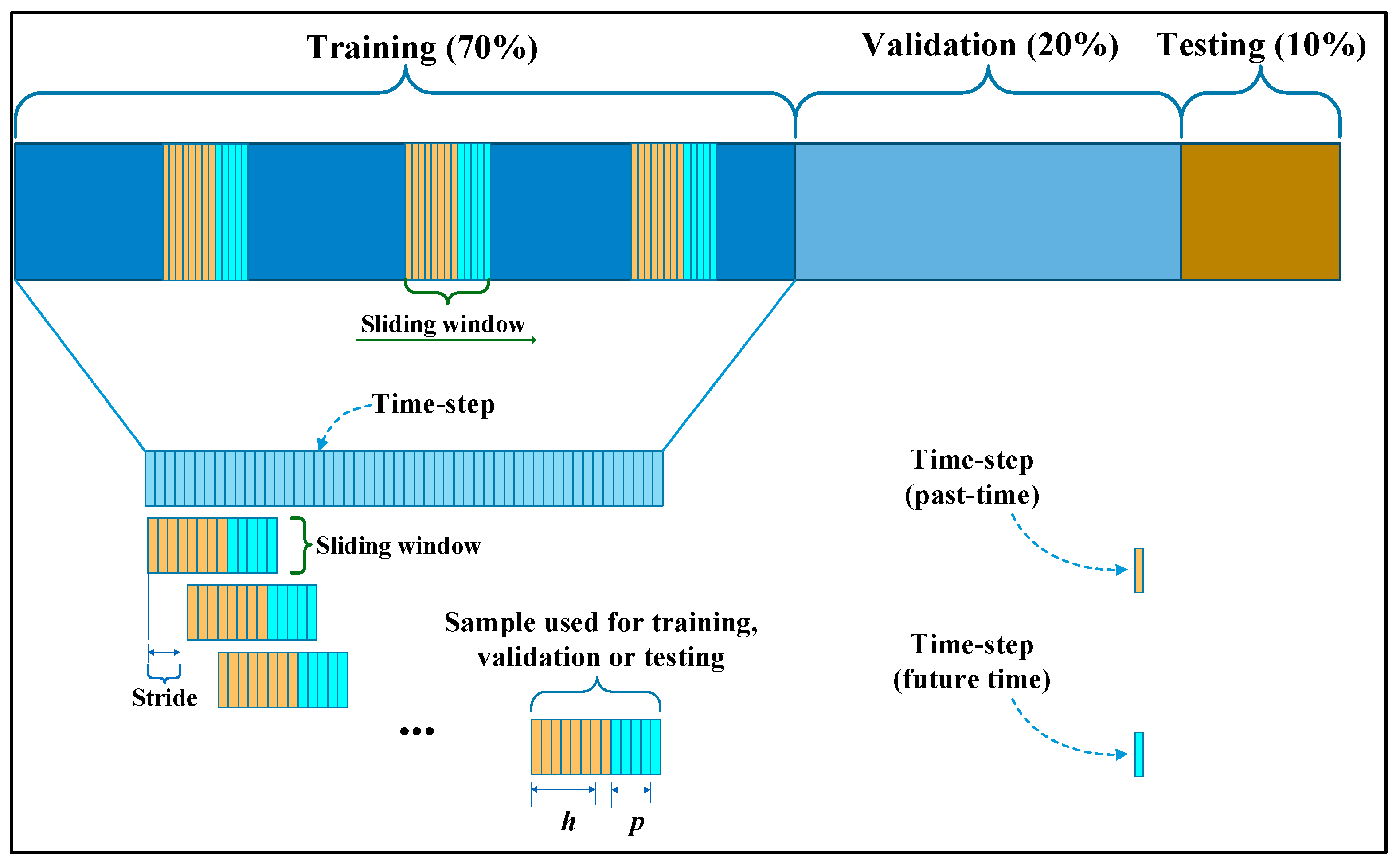
To comprehensively evaluate the performance of different models, it is essential to divide the wind speed data into training, validation, and testing sets. Figure 10 illustrates the process of data partitioning. A sliding window technique is utilized to segment the data into overlapping windows, obtaining multiple samples from a single time series. The stride of the sliding window is set to 1 in each experiment. Each sliding window consists of a combination of past-time slots and future-time time-ahead slots. The parameter h denotes the number of past-time slots, while the parameter p represents the number of future-time steps (i.e., the k-step ahead forecast length). In this study, the h and p are set to 32 and 1, respectively. Then, these data are divided into three sets, namely training data (70%), validation data (20%), and testing data (10%). The training data is used to train the sub-models within the CEEMDAN-LSTM model. The validation data is utilized to determine the optimal sub-model within the CEEMDAN-LSTM model. Finally, the testing data is designated to evaluate the prediction performance of the final CEEMDAN-LSTM model. In addition, all computations are executed on a computer equipped with a 9th generation AMD Ryzen 5950X @ 3.40 GHz processor from the United States and an NVIDIA RTX 3080Ti GPU. The neural networks are developed using Python 3.10 and the TensorFlow-GPU 2.10 deep learning framework, both from the United States.

3.4. Evaluation Indicators

To assess the performance of different models, several evaluation metrics are utilized for analysis, including the Mean Absolute Error (MAE) [42], Mean Square Error (MSE) [43], Root Mean Square Error (RMSE) [44], and Mean Absolute Percentage Error (MAPE). In addition, considering the normalized error metric as a relative measure eliminates the impact of scale, facilitating comparisons between different datasets. The Harmonic Mean Absolute Error (HMAE) [45], Harmonic Mean Squared Error (HMSE) [42], and Normalized Mean Square Error (NRMSE) are selected in this study. Lower values of MAE, MSE, RMSE, HMAE, HMSE, MAPE, and NRMSE indicate a smaller deviation between the predicted and original values. The evaluation indicators are presented as follows:
MAE = 1 n i = 1 n | y i y ^ i |
MSE = 1 n i = 1 n y i y ^ i 2
RMSE = i = 1 n ( y i y ^ i ) 2 / n
HMAE = i = 1 n | y i y ^ i | n / i = 1 n y ^ i n
HMSE = i = 1 n | y i y ^ i | n / ( i = 1 n y ^ i / n ) 2
MAPE = 100 % n i = 1 n | y i y ^ i y i |
NRMSE = 1 max ( y i ) min ( y i ) i = 1 n ( y i y ^ i ) 2 / n
where y ^ i and y i denote the prediction value and actual value. n represents the sum of all data points. In addition, the coefficient of determination (R2) exhibits the effectiveness of various prediction models [46]. R2 measures the proportion of the total variation in the dependent variable. It ranges from 0 to 1, where a value closer to 1 indicates a better fit of the model to the data, which is as follows:
R 2 = 1 SSE SST
where SSE (Sum of Squared Errors) is the sum of the squared differences between the predicted values and the actual values. SST (Total Sum of Squares) is the total sum of squares, which represents the total variation in the dependent variable.

4. Case Study

This section uses two cases to evaluate the effectiveness of the proposed CEEMDAN-LSTM method. Then, the study utilizes statistical tests to assess the significance of the performance differences between our proposed model and the benchmark models. Finally, a sensitivity analysis is conducted to identify the most critical factors affecting the proposed CEEMDAN-LSTM model’s performance.

4.1. Experiment 1: Wind Speed in Austria

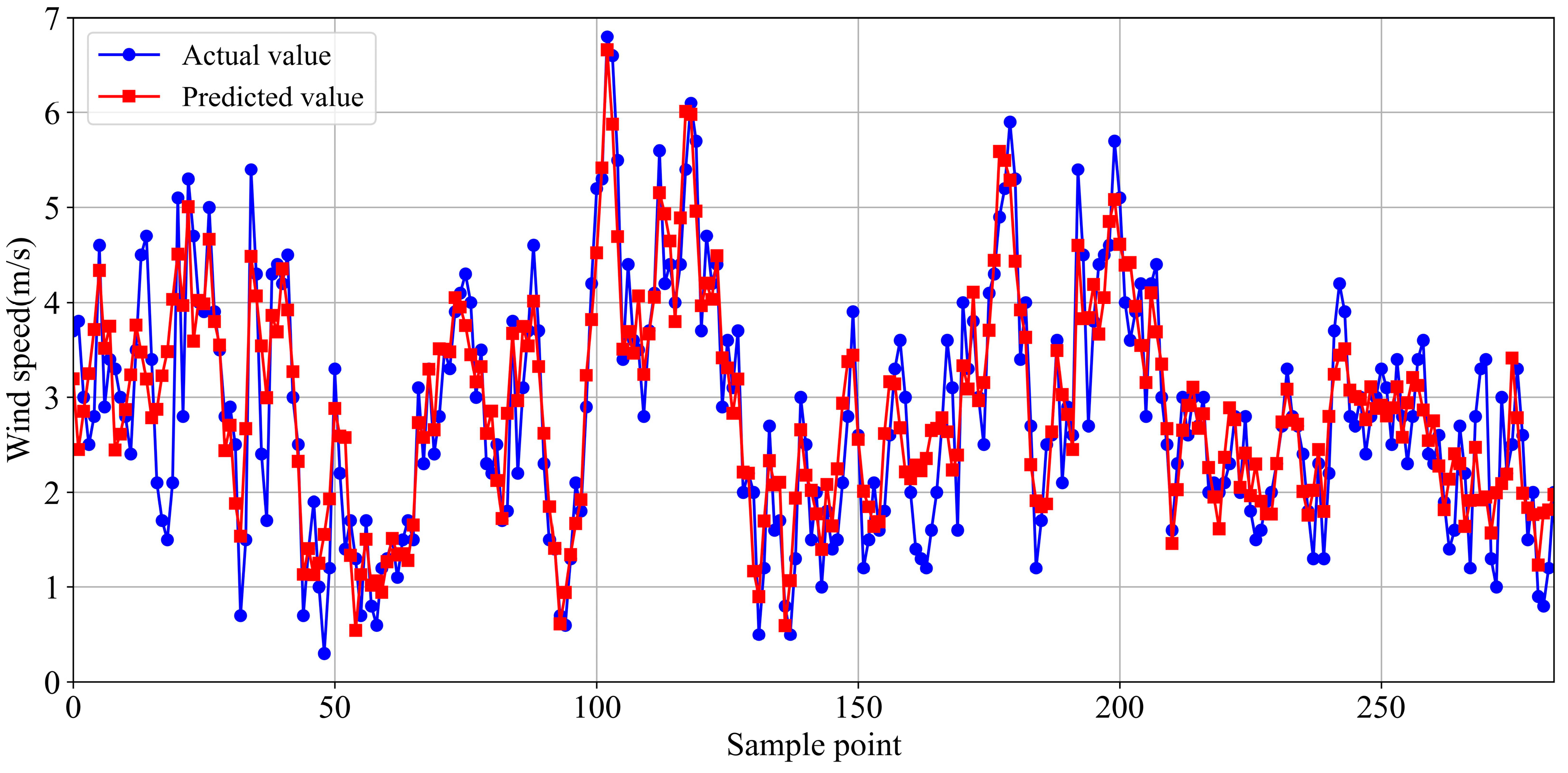
Figure 11 demonstrates the strong forecasting performance of the CEEMDAN-LSTM model for IMF2 through IMF9 and the Residual component, which show impressive alignment with the actual values. It indicates the model’s ability to capture the underlying patterns in these components effectively. The only exception is IMF1, in which the forecasts deviate visibly from the original data. This divergence is understandable given the high-frequency fluctuations in IMF1 that are inherently difficult to predict. Then, by summing up all IMFs and Res, the reconstructed wind speed curve can be obtained, as shown in Figure 12. For reconstructed wind speed, CEEMDAN-LSTM has a good overall fitting ability.
To evaluate the predicted performance of the reconstructed wind speed and every IMF with more accuracy, eight evaluated metrics, including R2, MAE, MSE, RMSE, HMAE, HMSE, MAPE, and NRMSE, are selected in Table 5. For the reconstructed wind speed, CEEMDAN-LSTM, with a strong correlation (R2 = 0.7952), shows a high prediction accuracy. Then, the error metrics of MAE in 0.4557, MSE in 0.3285, RMSE in 0.5732, MAPE in 0.2241, and NRMSE in 0.2020 are relatively low in absolute terms, showing that the model produces minor forecasting errors. The Harmonic HMAE in 0.1579 and HMSE in 0.0394 values are also relatively small, further indicating the model generates low errors for predicting wind speed. In addition, for other IMF components, IMF1 stands out with a relatively weak correlation (R2 = 0.0509) in prediction due to the high-frequency fluctuations that are inherently difficult to predict. IMF2 shows a strong correlation (R2 = 0.7956) and high accuracy. IMF3 to IMF8 show an almost perfect correlation (R2 ≈ 1) and outstanding accuracy, indicating that the model’s ability to capture the variations in these components accurately. In addition, the Res components exhibit a strong correlation (R2 = 0.9829), which demonstrates high accuracy. Overall, the CEEMDAN-LSTM demonstrates promising predictive abilities for wind speed.
To validate the performance of the CEEMDAN-LSTM model, comparative analyses are conducted against various benchmark models, namely DTR, SVR, DNN, LSTM, GRU, EMD-CNN, EMD-LSTM, and CEEMDAN-CNN. The testing dataset is utilized to evaluate the predictive capabilities of each model. Figure 13 displays the wind speed prediction results of the nine models. The upper part of the figure shows the predicted wind speeds (lines in different colors) and the actual wind speeds (blue line). To observe the prediction performance of the different models in detail, the lower part of the figure plots the scatter diagrams of the actual values versus the predicted values, which intuitively exhibits the prediction effectiveness of each model. For scatter diagrams, the red dot represents wind speed value and blue dash indicates the slope. The blue dashed line indicates a slope of 1, and the closer the scatters is to the blue dashed line, the closer the predicted values are to the actual values. The R2 values of the different prediction models are shown in the upper left corner of the scatter plots. From the R2 metric, it can be seen that the CEEMDAN-LSTM model achieves the best prediction performance, followed by CEEMDAN-CNN (R2 = 0.7716), EMD-LSTM (R2 = 0.7562), and EMD-CNN (R2 = 0.7526). Compared with these hybrid models, single modes, including DTR, SVR, DNN, LSTM, and GRU, have a general accuracy in predicting wind speed. Specifically, the GRU, LSTM, and DNN models attained R2 values of 0.5075, 0.5108, and 0.5027, respectively, indicating a moderate degree of fit between the forecasted and observed wind speed data. Conversely, the SVR and DTR models demonstrated the lowest R2 values of 0.4961 and 0.4360, respectively, which suggests a relatively limited efficacy. It can be found from the experimental results that these sequences, based on the CEEMDAN method decomposition, provide a better explanation of both long-term and short-term factors affecting power variations. The final wind speed prediction result is obtained by summing these predictions, which can improve the accuracy of the forecast compared with methods based on the original wind speed.
Some performance indicators are selected to verify the predicted result of different models, such as R2, MAE, MSE, RMSE, HMAE, HMSE, MAPE, and NRMSE in Figure 14 and Table 6. CEEMDAN-LSTM has the highest R2 score of 0.7952 and lowest values for MAE, MSE, RMSE, HMAE, HMSE, MAPE, and NRMSE, suggesting that it has the best overall performance among all the models listed. For the other hybrid models, it is observed that the CEEMDAN-CNN model achieves an R² value of 0.7716, while the EMD-LSTM and EMD-CNN models demonstrate comparable performance with R2 values of 0.7562 and 0.7526, respectively. These results indicate a close similarity in predictive accuracy. For LSTM and GRU, the two models have low performance with R2 scores of around 0.51, and relatively higher error rates than CEEMDAN-LSTM. DNN has an R2 score of 0.5027, which is slightly lower than that of LSTM and GRU. The SVR model has a slightly lower R2 score of 0.4961 compared to DNN, LSTM, and GRU. DTR has the lowest R2 score of 0.4360 and the highest error rates among all the models listed. Based on these metrics, the CEEMDAN-LSTM model demonstrates superior performance compared to the other models evaluated. This can be attributed to CEEMDAN’s ability to decompose the original wind speed data into a series of IMFs and a residual trend component. Such decomposition effectively breaks down the complex wind speed signal into simpler oscillatory modes that capture variations across different time scales, thereby allowing for the representation of both long-term trends and short-term fluctuations.

4.2. Experiment 2: Wind Speed in Almeria

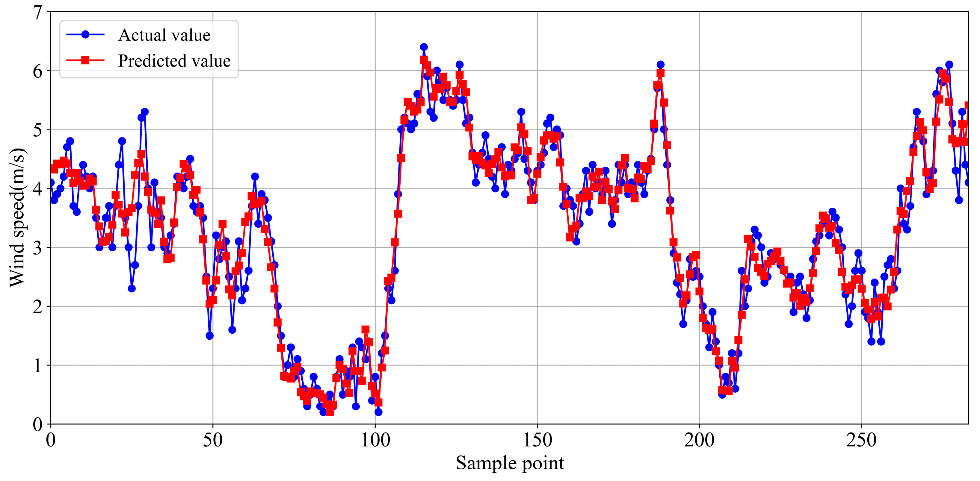
The predicted results of CEEMAN-LSTM are shown in Figure 15. The left half of the figure shows the comparison curve between the predicted wind speed (blue curve) and the actual wind speed (red curve). The closer the blue and red curves are, the better the prediction effect. The right side of the figure shows the loss curves of the components in the training and validation sets. As the number of iterations increases, the loss curve shows a decreasing trend and converges within 100 iterations. It is evident from the figure that the predicted values for IMF3 through IMF7 align closely with their actual values, while the predictions for IMF1 and IMF2 show discrepancies with the actual values. By summing all IMFs and Res obtained from CEEMDAN decomposition, the reconstructed wind speed is obtained in Figure 16.
To comprehensively analyze the prediction results of IMFs, Res, and reconstructed wind speed, eight evaluation metrics (R2, MAE, MSE, RMSE, HMAE, HMSE, MAPE, and NRMSE) are selected to evaluate the predictive capabilities of the CEEMDAN-LSTM model. Table 7 shows that IMF1 exhibits a minimal correlation with the actual data, as evidenced by its R2 value of merely 0.0017, suggesting a limited predictive prowess for high frequency. Then, a marked improvement in predictive accuracy is observed from IMF2 through IMF9. Notably, the R2 values for IMF3 to IMF7 are strikingly close to 1, indicating near-perfect predictions for these components. The Res component, with an R2 value of 0.9951, effectively captures the residual fluctuations, further emphasizing the model’s robustness. The error metrics for this reconstruction wind speed, with values such as MAE at 0.2980, MSE at 0.1455, and RMSE at 0.3815, are low, further highlighting the model’s high predictive precision.
To further investigate the effectiveness of the CEEMDAN-LSTM model in wind speed prediction, it is compared with different models, including DTR, SVR, DNN, LSTM, GRU, EMD-LSTM, EMD-CNN, and CEEMDAN-CNN. These models are evaluated using the same wind speed data to measure their predictive capabilities. The prediction results for each model are shown in Figure 17. The upper part of the figure displays the prediction trends of the different models on the test set, along with the actual wind speed data line plot. It can be observed that all models have performed well, with no significant deviations from the actual values. To further assess the prediction performance of each model, scatter plots of the predicted values versus the actual values are plotted below the figure. The scatter points are closer to the blue dashed line with a slope of 1, and the predicted values are closer to the actual values. Additionally, the scatter plot in the upper left corner marks the corresponding R2 value for each model, allowing for a straightforward comparison of the superiority of the CEEMDAN-LSTM in wind speed prediction. Experimental result shows that CEEMDAN-LSTM exhibits the highest R2 values of 0.9323 among all the models. Based on the above results, it can be observed that traditional methods struggle to predict future wind speed information from wind speed signals. Therefore, it is necessary to decompose complex nonlinear signals into several physically meaningful single-component signals, which enhances the frequency-domain resolution of signal analysis and improves the accuracy of wind speed prediction.
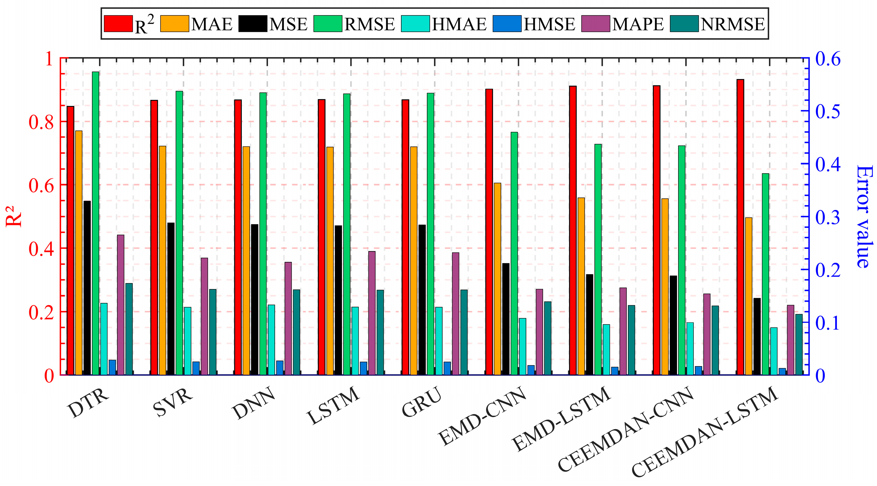
Detailed evaluation data for all the models on the test dataset are presented in Figure 18 and Table 8. The CEEMDAN-LSTM model achieved the best overall performance, with the highest R2 value of 0.9323 and the lowest error values across all metrics. This indicates that it had the best fit and accuracy in modeling the dataset. Subsequently, hybrid modes, including EMD-LSTM, EMD-CNN, and CEEMDAN-CNN, obtain better results for wind speed prediction. Specifically, the EMD-LSTM model achieves accuracy with an R2 value of 0.9112, effectively capturing wind speed variations. The CEEMDAN-CNN model, with the lowest relative error (HMSE of 0.0168), demonstrates superior stability and accuracy. The EMD-CNN model has a slightly lower performance, with an R2 value of 0.9017 and higher errors. In comparison, single models (such as DNN, LSTM, and GRU) have low prediction accuracy. The LSTM and GRU models, with R2 values of 0.8684 and 0.8678, are worse than CEEMDAN-LSTM. The DNN model performed similarly to LSTM and GRU. The SVR and DTR models achieved worse results across all metrics than the deep learning models. Their R2 values of 0.8660 and 0.8469 are the lowest, while their error values like MAE, MSE, and HMSE are the highest. In addition, when comparing the predictive performance of a single LSTM model with that of a combined model decomposed by the CEEMDAN algorithm, it was found that the hybrid model performed better. This is because wind speed data exhibits time series characteristics, and LSTM is more adept at capturing this relationship. Therefore, after multimodal decomposition, LSTM can better utilize the time series properties for prediction, learning features related to time dependency, and intermodal relationships from different IMF data. Thus, it can improve the prediction accuracy.

4.3. Statistical Analysis of Different Models

To assess the significance of performance differences, this study employs both the paired T-test [47] and the Wilcoxon signed-rank test [48] to compare the proposed CEEMDAN-LSTM model with various benchmark models, DTR, SVR, DNN, LSTM, GRU, EMD-CNN, EMD-LSTM, and CEEMDAN-CNN. Before proceeding with the statistical analyses, it is essential to verify whether the error distributions of each model meet the assumption of normality. The error is defined as follows:
error = y i y ^ i
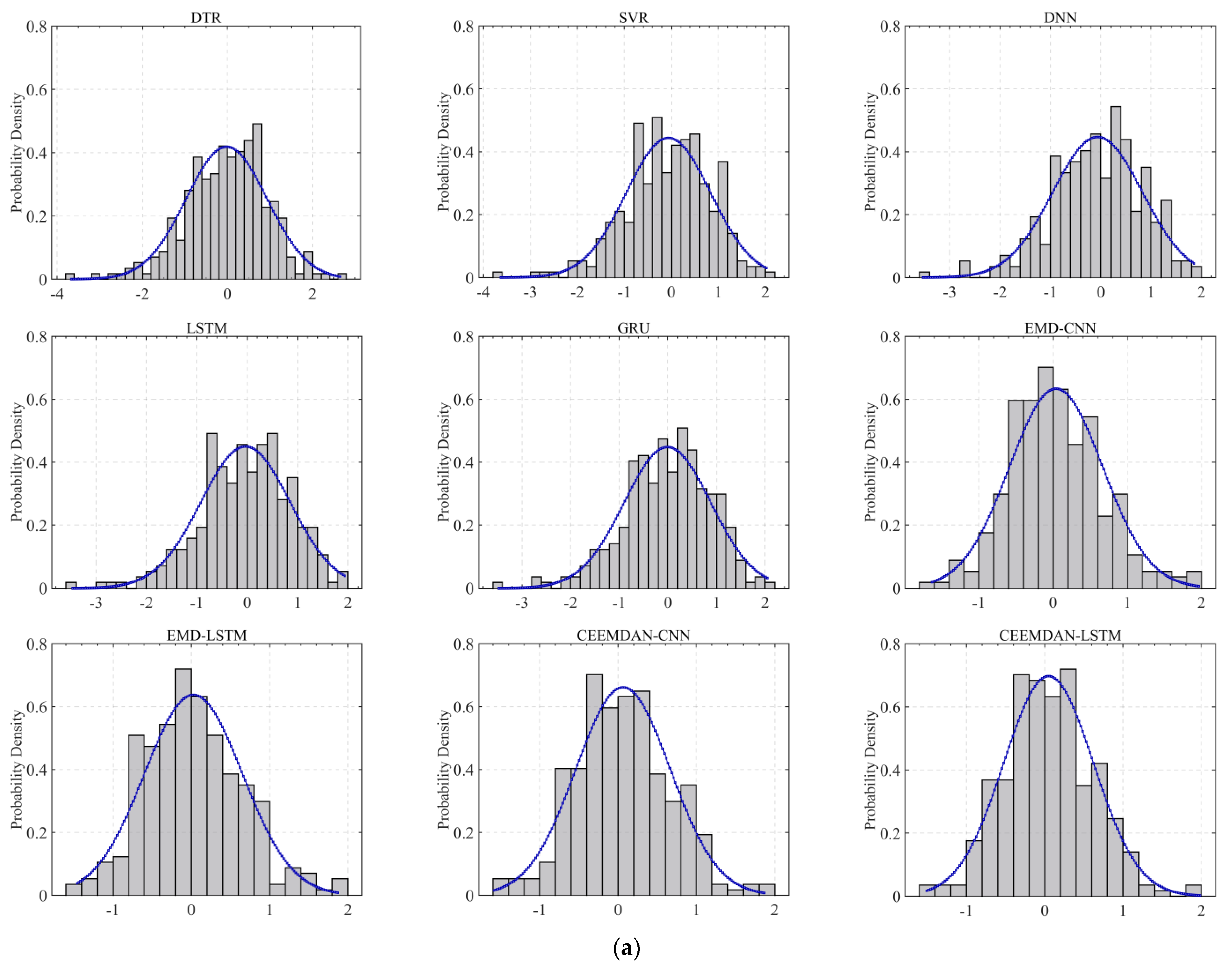
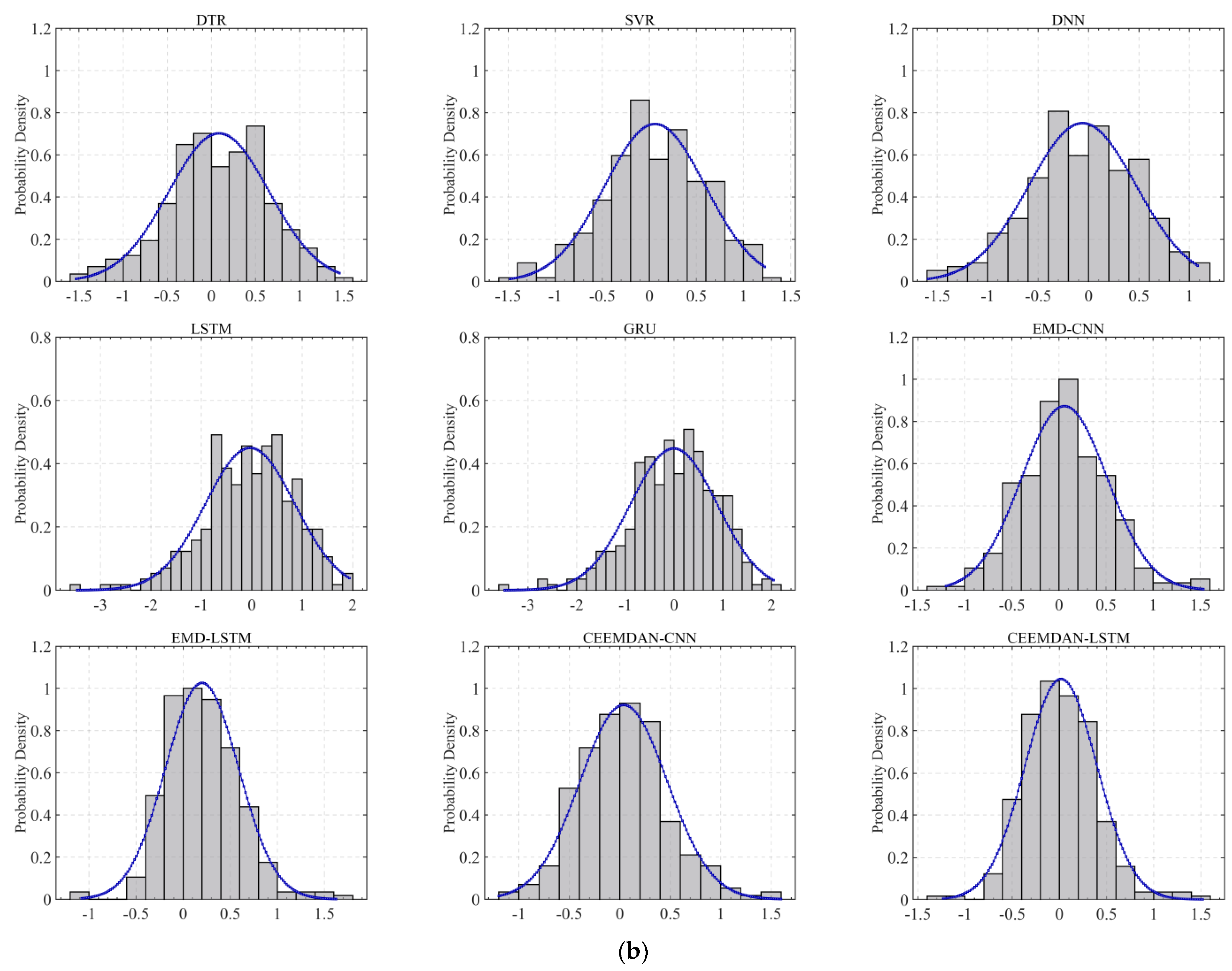
where y ^ i and y i denote the prediction value and actual value. If the error distribution satisfies the normal distribution, the paired T-test can be applied to determine whether there are significant differences between the model performances. Conversely, if the normality assumption is violated, the non-parametric Wilcoxon signed-rank test is conducted. The results of the normality tests for the different models’ error distributions are depicted in Figure 19 and Table 9.
Figure 19 shows error distribution on the testing dataset using different models, where the blue line represents fit curve. Table 9 shows the performance of different methods based on Paired t-test. Firstly, for the Austria dataset, the error distributions of CEEMDAN-CNN and CEEMDAN-LSTM meet the normality assumption, with p-values of 0.2461 and 0.2284, respectively. These p-values indicate that, at the 95% confidence level, the null hypothesis of normality cannot be rejected. In contrast, the error distributions of DTR, SVR, DNN, LSTM, GRU, EMD-CNN, and EMD-LSTM do not satisfy the normality assumption, as their p-values are all below the 0.05 threshold (0.0112, 0.0039, 0.0062, 0.0041, 0.0036, 0.0436, and 0.0429, respectively). Therefore, for these models, the Wilcoxon signed-rank test should be applied to determine the significance of the performance differences due to the violation of normality.
For the Almeria dataset, the error distributions of DTR, SVR, DNN, LSTM, GRU, and EMD-CNN satisfy the normality assumption, as indicated by their p-values (0.1083, 0.0999, 0.1825, 0.2689, 0.3194, and 0.0807, respectively), which are above the 0.05 threshold. However, EMD-LSTM, CEEMDAN-CNN, and CEEMDAN-LSTM show p-values of 0.0005, 0.0076, and 0.0003, respectively, indicating non-normal distributions. In summary, for models that satisfy the normality assumption, the paired T-test is appropriate, while for those that do not, the Wilcoxon signed-rank test is more suitable.
For most models, including DTR, SVR, DNN, LSTM, GRU, EMD-CNN, CEEMDAN-CNN, and CEEMDAN-LSTM, the p-values are greater than 0.05 for both datasets. This indicates that there is no statistically significant difference in the performance between these models and the baseline models. However, the EMD-LSTM model shows a very low p-value (2.9684 × 10⁻¹⁵) on the Almeria dataset, suggesting a highly significant difference compared to the baseline.
In addition, the proposed CEEMDAN-LSTM model stands out due to its robust performance across both datasets in Table 10. Specifically, the CEEMDAN technique decomposes the complex nonlinear signals into several physically meaningful single-component signals, leading to more reliable features for the LSTM model to learn. This is particularly adept at handling time series data; the proposed CEEMDAN-LSTM model can capture long-term dependencies and temporal patterns effectively. While other models show similar performance levels, the proposed CEEMDAN-LSTM model consistently demonstrates non-significant differences (p > 0.05), indicating that its performance is comparable to or better than that of existing methods without introducing additional variance or bias.

4.4. Computational Efficiency and Sensitivity Analysis

Table 11 presents a comparative analysis of the prediction times of various models for the testing datasets, highlighting the performance differences across several machine learning and deep learning algorithms. The models include DTR, SVR, DNN, LSTM, GRU, EMD-CNN, EMD-LSTM, CEEMDAN-CNN, and CEEMDAN-LSTM.
Among these models, the proposed CEEMDAN-LSTM model, which integrates the CEEMDAN and LSTM networks, demonstrates a competitive prediction time, particularly in relation to other deep learning models. For the Austria dataset, CEEMDAN-LSTM exhibits a prediction time of 0.228 s, which is shorter than both the standalone LSTM (0.256 s) and GRU (0.241 s), and comparable to EMD-LSTM (0.231 s). For the Almeria dataset, CEEMDAN-LSTM achieves a prediction time of 0.227 s, outperforming LSTM (0.303 s) and GRU (0.294 s), and again showing similar efficiency to EMD-LSTM (0.229 s).
These results suggest that the CEEMDAN-LSTM model strikes a favorable balance between computational efficiency and model complexity, potentially offering superior performance in scenarios in which both accuracy and prediction speed are crucial. The integration of CEEMDAN in the model architecture enhances the decomposition process, which could contribute to its relatively lower computational time compared to other LSTM-based approaches. Thus, the CEEMDAN-LSTM model is a promising candidate for time-sensitive predictive modeling tasks.
Table 12 presents the experimental results of the CEEMDAN-LSTM model on the Austria and Almeria datasets, where three key hyperparameters—sliding window size, number of neurons in the LSTM layer, and number of neurons in the fully connected layer—are varied. The model’s performance is evaluated using four metrics: R2, HMSE, MAPE, and NRMSE.
The results reveal that the model’s predictive performance is highly sensitive to the choice of these parameters. Notably, the optimal results are achieved when the Window size is set to 15, the number of neurons in the LSTM layer is 16, and the number of neurons in the fully connected layer is 5. Under these specific configurations, the CEEMDAN-LSTM model achieves the highest R2 values (0.7952 for the Austria dataset and 0.9323 for the Almeria dataset), indicating the best goodness-of-fit between the predicted and actual values. Simultaneously, the lowest error metrics, HMSE (0.0394 for Austria, 0.0131 for Almeria), MAPE (0.2241 for Austria, 0.1323 for Almeria), and NRMSE (0.2020 for Austria, 0.1152 for Almeria), suggest that the CEEMDAN-LSTM model is both accurate and reliable in its predictions.
When the Window size is set to values other than 15 (e.g., 5, 10, 20, and 30), a notable decrease in R2 and an increase in error metrics are observed across both datasets. This suggests that a Window size of 15 captures the temporal dependencies in the time series data more effectively, balancing model complexity and overfitting. Similarly, variations in the number of neurons in the LSTM layer show that 16 neurons result in the most effective learning capacity, optimizing the balance between underfitting and overfitting. Lower or higher values (e.g., 10, 32, 50, and 64) lead to slightly decreased R2 values and higher error metrics, indicating less optimal model performance. Furthermore, the number of neurons in the fully connected layer is critical for achieving optimal results. With a value of 5, the model achieves the best performance metrics on both datasets. Increasing or decreasing the number of neurons (e.g., 3, 10, 15, and 30) results in marginally lower performance, suggesting that five neurons provide the necessary network capacity to adequately map the features extracted by the LSTM layer to the final output without unnecessary complexity.
The specific combination of a Window size of 15, 16 neurons in the LSTM layer and five neurons in the fully connected layer achieves a balance that minimizes prediction errors while maximizing the R2, thus offering a robust model configuration for both the Austria and Almeria datasets.

5. Conclusions and Future Work

This study proposes a new modeling framework based on CEEMDAN-LSTM for wind speed forecasting. The effectiveness of the proposed model is verified by real-world wind speed data in Austria and Almeria. The main findings of the present study are summarized as follows:
(1)
Compared with traditional wind speed forecasting methods (e.g., LSTM and GRU), the CEEMDAN-LSTM model can extract the multiscale temporal properties of wind speed data, which can considerably improve the accuracy of wind speed forecasting.
(2)
CEEMDAN is highly effective in reducing the nonlinearity present in wind speed data; integrating CEEMDAN into the LSTM model results in significantly superior performance. For LSTM-based models, the R2 value can be substantially increased by 28.44% for Austria and 6.39% for Almeria, following the application of CEEMDAN.
(3)
The proposed model achieves a significant improvement in wind speed forecasting compared with the five benchmark models. The MSE value of the CEEMDAN-LSTM model is reduced by at least 240% and 195% for Austria and Almeria, respectively, compared with the single models (e.g., DTR, SVR, DNN, LSTM, and GRU). In addition, for some catastrophe points, the CEEMDAN-LSTM model can still obtain more accurate predictions.
(4)
By analyzing different hyperparameters of CEEMDAN-LSTM, including sliding window size, neuron number of LSTM layer, and fully connected layer, the experimental results demonstrate that a Window size of 15, 16 neurons in the LSTM layer, and five neurons in the fully connected layer achieves a balance that minimizes prediction errors.
Limitation and future work: The proposed framework in this study is entirely data-driven, relying exclusively on data for analysis and forecasting. Thus, this approach can exhibit lower accuracy in wind speed forecasting within complex environments, owing to the disregard of physical information in reality. In future research work, we intend to integrate physical information or physical laws into deep learning models to enhance both the accuracy and interpretability of wind speed forecasting.

Author Contributions

The authors confirm their contribution to the paper as follows: draft manuscript preparation: Y.H.; data collection: T.G.; analysis and interpretation of results: Z.Z.; methodology: L.Z.; funding acquisition: Y.H. All authors have read and agreed to the published version of the manuscript.

Funding

This research was funded by the Science and Technology Research Program of Chongqing Municipal Education Commission (Grant No. KJQN202201805, KJQN202301801, KJZD-M202201801, KJQN202303114), the Science and Technology Research Program of Chongqing College of Humanities, Science & Technology (Grant No. CRKZK2023007, JSJGC202201). Research Center for Big Data and Network Information Security Engineering Technology of Chongqing College of Humanities, Science & Technology.

Data Availability Statement

The datasets generated during the analysis are available from the corresponding author.

Acknowledgments

We would like to express our heartfelt gratitude to the esteemed reviewers for their invaluable contributions to the refinement of this scientific manuscript.

Conflicts of Interest

The authors declare that they have no conflicts of interest.

References

  1. Więckowski, J.; Kizielewicz, B.; Sałabun, W. A Multi-Dimensional Sensitivity Analysis Approach for Evaluating the Robustness of Renewable Energy Sources in European Countries. J. Clean. Prod. 2024, 469, 143225. [Google Scholar] [CrossRef]
  2. Wilberforce, T.; Olabi, A.G.; Sayed, E.T.; Mahmoud, M.; Alami, A.H.; Abdelkareem, M.A. The State of Renewable Energy Source Envelopes in Urban Areas. Int. J. Thermofluids 2024, 21, 100581. [Google Scholar] [CrossRef]
  3. Gong, Z.; Wan, A.; Ji, Y.; AL-Bukhaiti, K.; Yao, Z. Improving Short-Term Offshore Wind Speed Forecast Accuracy Using a VMD-PE-FCGRU Hybrid Model. Energy 2024, 295, 131016. [Google Scholar] [CrossRef]
  4. Yang, M.; Han, C.; Zhang, W.; Wang, B. A Short-Term Power Prediction Method for Wind Farm Cluster Based on the Fusion of Multi-Source Spatiotemporal Feature Information. Energy 2024, 294, 130770. [Google Scholar] [CrossRef]
  5. Gielen, D.; Boshell, F.; Saygin, D.; Bazilian, M.D.; Wagner, N.; Gorini, R. The role of renewable energy in the global energy transformation. Energy Strategy Rev. 2019, 24, 38–50. [Google Scholar] [CrossRef]
  6. Zhao, X.; Sun, B.; Wu, N.; Zeng, R.; Geng, R.; He, Z. A New Short-Term Wind Power Prediction Methodology Based on Linear and Nonlinear Hybrid Models. Comput. Ind. Eng. 2024, 196, 110477. [Google Scholar] [CrossRef]
  7. Cobos-Maestre, M.; Flores-Soriano, M.F.; Barrero, D. SWAN: A Multihead Autoregressive Attention Model for Solar Wind Speed Forecasting. Expert Syst. Appl. 2024, 252, 124128. [Google Scholar] [CrossRef]
  8. Yang, B.; Zhu, H.; Zhang, Q.; Wüchner, R.; Sun, S.; Qiu, J. Identification of Wind Loads on a 600 m High Skyscraper by Kalman Filter. J. Build. Eng. 2023, 63, 105440. [Google Scholar] [CrossRef]
  9. Yunus, K.; Thiringer, T.; Chen, P. ARIMA-Based Frequency-Decomposed Modeling of Wind Speed Time Series. IEEE Trans. Power Syst. 2016, 31, 2546–2556. [Google Scholar] [CrossRef]
  10. Xie, W.; Zhang, P.; Chen, R.; Zhou, Z. A Nonparametric Bayesian Framework for Short-Term Wind Power Probabilistic Forecast. IEEE Trans. Power Syst. 2019, 34, 371–379. [Google Scholar] [CrossRef]
  11. Wang, J.; Li, H.; Wang, Y.; Lu, H. A hesitant fuzzy wind speed forecasting system with novel defuzzification method and multi-objective optimization algorithm. Expert Syst. Appl. 2021, 168, 114364. [Google Scholar] [CrossRef]
  12. Huang, C.; Karimi, H.R.; Mei, P.; Yang, D.; Shi, Q. Evolving Long Short-Term Memory Neural Network for Wind Speed Forecasting. Inf. Sci. 2023, 632, 390–410. [Google Scholar] [CrossRef]
  13. Chen, G.; Tang, B.; Zeng, X.; Zhou, P.; Kang, P.; Long, H. Short-Term Wind Speed Forecasting Based on Long Short-Term Memory and Improved BP Neural Network. Int. J. Electr. Power Energy Syst. 2022, 134, 107365. [Google Scholar] [CrossRef]
  14. Xie, C.; Yang, X.; Chen, T.; Fang, Q.; Wang, J.; Shen, Y. Short-Term Wind Power Prediction Framework Using Numerical Weather Predictions and Residual Convolutional Long Short-Term Memory Attention Network. Eng. Appl. Artif. Intell. 2024, 133, 108543. [Google Scholar] [CrossRef]
  15. Zheng, Y.; Ge, Y.; Muhsen, S.; Wang, S.; Elkamchouchi, D.H.; Ali, E.; Ali, H.E. New Ridge Regression, Artificial Neural Networks and Support Vector Machine for Wind Speed Prediction. Adv. Eng. Softw. 2023, 179, 103426. [Google Scholar] [CrossRef]
  16. Wang, Z.; Li, G.; Yao, L.; Cai, Y.; Lin, T.; Zhang, J.; Dong, H. Intelligent Fault Detection Scheme for Constant-Speed Wind Turbines Based on Improved Multiscale Fuzzy Entropy and Adaptive Chaotic Aquila Optimization-Based Support Vector Machine. ISA Trans. 2023, 138, 582–602. [Google Scholar] [CrossRef]
  17. Zhu, A.; Zhao, Q.; Yang, T.; Zhou, L.; Zeng, B. Wind Speed Prediction and Reconstruction Based on Improved Grey Wolf Optimization Algorithm and Deep Learning Networks. Comput. Electr. Eng. 2024, 114, 109074. [Google Scholar] [CrossRef]
  18. Zameer, A.; Arshad, J.; Khan, A.; Raja, M.A.Z. Intelligent and robust prediction of short term wind power using genetic programming based ensemble of neural networks. Energy Convers. Manag. 2017, 134, 361–372. [Google Scholar] [CrossRef]
  19. Jiang, P.; Liu, Z.; Niu, X.; Zhang, L. A Combined Forecasting System Based on Statistical Method, Artificial Neural Networks, and Deep Learning Methods for Short-Term Wind Speed Forecasting. Energy 2021, 217, 119361. [Google Scholar] [CrossRef]
  20. Shahid, F.; Zameer, A.; Mehmood, A.; Raja, M.A.Z. A novel wavenets long short term memory paradigm for wind power prediction. Appl. Energy 2020, 269, 115098. [Google Scholar] [CrossRef]
  21. Liu, H.; Yang, R.; Wang, T.; Zhang, L. A hybrid neural network model for short-term wind speed forecasting based on decomposition, multi-learner ensemble, and adaptive multiple error corrections. Renew. Energy 2021, 165, 573–594. [Google Scholar] [CrossRef]
  22. Li, D.; Jiang, F.; Chen, M.; Qian, T. Multi-Step-Ahead Wind Speed Forecasting Based on a Hybrid Decomposition Method and Temporal Convolutional Networks. Energy 2022, 238, 121981. [Google Scholar] [CrossRef]
  23. Li, Z.; Xu, R.; Luo, X.; Cao, X.; Sun, H. Short-Term Wind Power Prediction Based on Modal Reconstruction and CNN-BiLSTM. Energy Rep. 2023, 9, 6449–6460. [Google Scholar] [CrossRef]
  24. Chen, Y.; Dong, Z.; Wang, Y.; Su, J.; Han, Z.; Zhou, D.; Zhang, K.; Zhao, Y.; Bao, Y. Short-Term Wind Speed Predicting Framework Based on EEMD-GA-LSTM Method under Large Scaled Wind History. Energy Convers. Manag. 2021, 227, 113559. [Google Scholar] [CrossRef]
  25. Zhang, Y.; Chen, Y. Application of Hybrid Model Based on CEEMDAN, SVD, PSO to Wind Energy Prediction. Environ. Sci. Pollut. Res. 2022, 29, 22661–22674. [Google Scholar] [CrossRef]
  26. Ding, Y.; Chen, Z.; Zhang, H.; Wang, X.; Guo, Y. A Short-Term Wind Power Prediction Model Based on CEEMD and WOA-KELM. Renew. Energy 2022, 189, 188–198. [Google Scholar] [CrossRef]
  27. Qu, Z.; Zhang, K.; Mao, W.; Wang, J.; Liu, C.; Zhang, W. Research and application of ensemble forecasting based on a novel multi-objective optimization algorithm for wind-speed forecasting. Energy Convers. Manag. 2017, 154, 440–454. [Google Scholar] [CrossRef]
  28. Jaseena, K.U.; Kovoor, B.C. Decomposition-based hybrid wind speed forecasting model using deep bidirectional LSTM networks. Energy Convers. Manag. 2021, 234, 113944. [Google Scholar] [CrossRef]
  29. Shahid, F.; Zameer, A.; Muneeb, M. A novel genetic LSTM model for wind power forecast. Energy 2021, 223, 120069. [Google Scholar] [CrossRef]
  30. Yang, D.; Li, M.; Guo, J.; Du, P. An Attention-Based Multi-Input LSTM with Sliding Window-Based Two-Stage Decomposition for Wind Speed Forecasting. Appl. Energy 2024, 375, 124057. [Google Scholar] [CrossRef]
  31. Liu, W.; Bai, Y.; Yue, X.; Wang, R.; Song, Q. A Wind Speed Forcasting Model Based on Rime Optimization Based VMD and Multi-Headed Self-Attention-LSTM. Energy 2024, 294, 130726. [Google Scholar] [CrossRef]
  32. Wang, J.; Niu, X.; Zhang, L.; Liu, Z.; Huang, X. A Wind Speed Forecasting System for the Construction of a Smart Grid with Two-Stage Data Processing Based on Improved ELM and Deep Learning Strategies. Expert Syst. Appl. 2024, 241, 122487. [Google Scholar] [CrossRef]
  33. Priyadarshini, I.; Cotton, C. A novel LSTM–CNN–grid search-based deep neural network for sentiment analysis. J. Supercomput. 2021, 77, 13911–13932. [Google Scholar] [CrossRef]
  34. Veynandt, F.; Inschlag, F.; Seidl, C.; Heschl, C. Measurement dataset from real operation of a hybrid photovoltaic-thermal solar collectors, used for the development of a data-driven model. Data Brief 2023, 49, 109417. [Google Scholar] [CrossRef]
  35. Acharya, S.; Adamová, D.; Aglieri Rinella, G.; Agnello, M.; Agrawal, N.; Ahammed, Z.; Ahmad, S.; Ahn, S.U.; Ahuja, I.; Akindinov, A.; et al. Skewness and Kurtosis of Mean Transverse Momentum Fluctuations at the LHC Energies. Phys. Lett. B 2024, 850, 138541. [Google Scholar] [CrossRef]
  36. De Luca, D.L.; Ridolfi, E.; Russo, F.; Moccia, B.; Napolitano, F. Climate Change Effects on Rainfall Extreme Value Distribution: The Role of Skewness. J. Hydrol. 2024, 634, 130958. [Google Scholar] [CrossRef]
  37. Yuzgec, U.; Dokur, E.; Balci, M. A Novel Hybrid Model Based on Empirical Mode Decomposition and Echo State Network for Wind Power Forecasting. Energy 2024, 300, 131546. [Google Scholar] [CrossRef]
  38. Huo, J.; Xu, J.; Chang, C.; Li, C.; Qi, C.; Li, Y. Ultra-Short-Term Wind Power Prediction Model Based on Fixed Scale Dual Mode Decomposition and Deep Learning Networks. Eng. Appl. Artif. Intell. 2024, 133, 108501. [Google Scholar] [CrossRef]
  39. Zapata-Sierra, A.J.; Cama-Pinto, A.; Montoya, F.G.; Alcayde, A.; Manzano-Agugliaro, F. Wind missing data arrangement using wavelet based techniques for getting maximum likelihood. Energy Convers. Manag. 2019, 185, 552–561. [Google Scholar] [CrossRef]
  40. Kumar, B.; Yadav, N. A Novel Hybrid Algorithm Based on Empirical Fourier Decomposition and Deep Learning for Wind Speed Forecasting. Energy Convers. Manag. 2024, 300, 117891. [Google Scholar] [CrossRef]
  41. Singh, S.K.; Jha, S.K.; Gupta, R. Enhancing the Accuracy of Wind Speed Estimation Model Using an Efficient Hybrid Deep Learning Algorithm. Sustain. Energy Technol. Assess. 2024, 61, 103603. [Google Scholar] [CrossRef]
  42. Khan, A.W.; Duan, J.; Nawaz, F.; Lu, W.; Han, Y.; Ma, W. Innovative Hybrid NARX-RNN Model for Predicting Wind Speed to Harness Wind Power in Pakistan. Energy Rep. 2024, 12, 2373–2387. [Google Scholar] [CrossRef]
  43. Du, P.; Yang, D.; Li, Y.; Wang, J. An Innovative Interpretable Combined Learning Model for Wind Speed Forecasting. Appl. Energy 2024, 358, 122553. [Google Scholar] [CrossRef]
  44. Sareen, K.; Panigrahi, B.K.; Shikhola, T.; Chawla, A. A Robust De-Noising Autoencoder Imputation and VMD Algorithm Based Deep Learning Technique for Short-Term Wind Speed Prediction Ensuring Cyber Resilience. Energy 2023, 283, 129080. [Google Scholar] [CrossRef]
  45. Saidin, S.S.; Kudus, S.A.; Jamadin, A.; Anuar, M.A.; Amin, N.M.; Ya, A.B.Z.; Sugiura, K. Vibration-Based Approach for Structural Health Monitoring of Ultra-High-Performance Concrete Bridge. Case Stud. Constr. Mater. 2023, 18, e01752. [Google Scholar] [CrossRef]
  46. Akgül, F.G.; Şenoğlu, B. Comparison of Wind Speed Distributions: A Case Study for Aegean Coast of Turkey. Energy Source Part A Recover. Util. Environ. Eff 2023, 45, 2453–2470. [Google Scholar] [CrossRef]
  47. Okoye, K.; Hosseini, S. T-Test Statistics in R: Independent Samples, Paired Sample, and One Sample T-Tests. In R Programming; Springer Nature: Singapore, 2024; pp. 159–186. ISBN 978-981-9733-84-2. [Google Scholar]
  48. Li, X.; Wu, Y.; Wei, M.; Guo, Y.; Yu, Z.; Wang, H.; Li, Z.; Fan, H. A Novel Index of Functional Connectivity: Phase Lag Based on Wilcoxon Signed Rank Test. Cogn Neurodyn 2021, 15, 621–636. [Google Scholar] [CrossRef]
Figure 1. Framework of wind speed forecasting based on CEEMDAN-LSTM method.
Energies 17 04615 g001
Figure 2. Decomposed process of CEEMDAN method.
Energies 17 04615 g002
Figure 3. Graphical representation of an LSTM cell.
Energies 17 04615 g003
Figure 4. Locations of the wind speed sensor.
Energies 17 04615 g004
Figure 5. Raw wind speed in Austria area.
Energies 17 04615 g005
Figure 6. CEEMDAN decomposition of the wind speed (Austria dataset).
Energies 17 04615 g006
Figure 7. Map of the Almeria city, Spain, Andalusia.
Energies 17 04615 g007
Figure 8. Raw wind speed in Almeria.
Energies 17 04615 g008
Figure 9. CEEMDAN decomposition of the wind speed (Almeria dataset).
Energies 17 04615 g009
Figure 10. Data partitioning process of wind speed data.
Energies 17 04615 g010
Figure 11. Predicted result of IMF modes using the CEEMDAN-LSTM model (Austria dataset).
Energies 17 04615 g011
Figure 12. Forecasting result of wind speed on the testing dataset based on the CEEMDAN-LSTM model (Austria dataset).
Energies 17 04615 g012
Figure 13. Forecasting results on the testing dataset using different models (Austria dataset).
Energies 17 04615 g013
Figure 14. Evaluation results on the testing dataset using different models (Austria dataset).
Energies 17 04615 g014
Figure 15. Predicted result of IMF modes curves using the CEEMDAN-LSTM model (Almeria dataset).
Energies 17 04615 g015
Figure 16. Forecasting result of wind speed on the testing dataset based on the CEEMDAN-LSTM model (Almeria dataset).
Energies 17 04615 g016
Figure 17. Forecasting results on the testing dataset using the different models (Almeria dataset).
Energies 17 04615 g017
Figure 18. Evaluation results on the testing dataset using different models (Almeria dataset).
Energies 17 04615 g018
Figure 19. Error distribution on the testing dataset using different models. (a) Error distribution for different models (Austria dataset). (b) Error distribution for different models (Almeria dataset).
Energies 17 04615 g019aEnergies 17 04615 g019b
Table 1. Grid search hyperparameters for CEEMDAN-LSTM Model.
HyperparametersRange of ValuesOptimal Value
Batch size16, 32, 6432
Learning rate0.01, 0.005, 0.001, 0.0005, 0.00025, 0.00010.0001
Drop regularization0.1, 0.2, 0.4, 0.6, 0.70.2
First-layer LSTM neurons10, 16, 32, 64, 12816
Fully connected neurons5, 10, 15, 30, 505
Table 2. Grid search parameters for comparison model.
Comparison ModelsParametersRange of ValuesOptimal Value
DTRMax depthNone, 5, 10, 15, 205
Min samples split2, 5, 102
Min samples leaf1, 2, 45
SVRRegularization parameter0.1, 1, 10, 10010
Gamma‘scale’, ‘auto’‘scale’
Kernel‘linear’, ‘rbf’, ‘poly’‘linear’
DNNNumber of neurons in the first layer5, 10, 15, 30, 50, 80, 10050
Number of neurons in the second layer5, 10, 15, 30, 50, 80, 10030
LSTMNumber of neurons in the LSTM layer10, 16, 32, 64, 12816
Number of neurons in fully connected layer5, 10, 15, 30, 505
GRUNumber of neurons in the GRU layer10, 16, 32, 64, 12864
Number of neurons in fully connected layer5, 10, 15, 30, 5050
EMD-LSTMNumber of neurons in the LSTM layer10, 16, 32, 6416
Number of neurons in fully connected layer5, 10, 15, 30, 505
EEMD-CNNFilter number of convolution layer4, 8, 12, 16, 20, 24, 2812
Number of neurons in fully connected layer5, 10, 15, 30, 5015
CEEMDAN-CNNFilter number of convolution layer4, 8, 12, 16, 20, 24, 2816
Number of neurons in fully connected layer5, 10, 15, 30, 5010
CEEMDAN-LSTMNumber of neurons in the LSTM layer10,16,32,6416
Number of neurons in fully connected layer5, 10, 15, 30, 505
Table 3. Statistical analysis of IMF modes for wind speed (Austria dataset).
DecompositionMaxMinMeanStdSkewKurtosis
IMF11.7813−1.7589−0.00510.5112−0.0324−0.2095
IMF21.6128−1.4457−0.00460.44090.02330.2994
IMF32.9989−2.63920.00330.56420.06751.6327
IMF41.4569−1.4984−0.01330.4755−0.12220.0930
IMF51.0717−0.91840.00260.30720.08120.8072
IMF60.8470−0.9359−0.00550.2788−0.07640.5749
IMF70.5248−0.7065−0.02080.2146−0.45811.0574
IMF80.5658−0.55260.08460.3251−0.1903−1.0986
Res2.92572.15162.68050.2196−1.03820.1547
Table 4. Statistical analysis of IMF modes for wind speed (Almeria dataset).
DecompositionMaxMinMeanStdSkewKurtosis
IMF11.7985−1.82490.00480.38340.04401.6042
IMF23.1774−3.35400.00160.41270.023510.2940
IMF32.7972−2.26570.00890.55540.24192.3542
IMF42.1434−2.3087−0.02040.6906−0.13251.0496
IMF53.5188−4.3391−0.02381.0021−0.12112.0020
IMF62.8737−2.87030.04791.01610.02220.2478
IMF72.7397−2.9049−0.19021.36330.0385−0.8332
IMF81.6011−1.50580.12940.88930.0118−1.1827
Res4.90844.33414.55280.21620.5321−1.3657
Table 5. The evaluation metrics of the proposed CEEMDAN-LSTM model.
CEEMDAN-LSTMR2MAEMSERMSEHMAEHMSEMAPENRMSE
IMF10.05090.43100.30690.5540−144.899034688.77491.6497−35.4056
IMF20.79560.15940.04390.209617.5991535.58131.7780−8.8675
IMF30.99430.02950.00170.04132.928616.77880.21986.0853
IMF40.99990.00219.37 × 10−60.0031−0.04340.00380.0085−0.0635
IMF50.99990.00054.58 × 10−70.00070.02230.00080.00630.0286
IMF60.99980.00042.49 × 10−70.0005−0.01170.00020.0038−0.0131
IMF70.99980.00111.28 × 10−60.0011−0.00421.89 × 10−50.0043−0.0043
IMF80.99970.00022.51 × 10−80.00020.00038.59 × 10−80.00030.0003
Rse0.98290.00053.44 × 10−70.00060.00024.89 × 10−80.00020.0002
Reconstructed wind speed0.79520.45570.32850.57320.15790.03940.22410.2020
Table 6. The evaluated result of the testing dataset using various models.
ModelsR2MAEMSERMSEHMAEHMSEMAPENRMSE
DTR0.43600.75050.90490.95130.26620.11380.34660.3353
SVR0.49610.71310.80850.89920.25700.10500.33370.3169
DNN0.50270.70690.79790.89330.25480.10370.32790.3148
LSTM0.51080.70310.78490.88590.25080.09990.33240.3123
GRU0.50750.70510.79010.88890.24900.09860.33670.3133
EMD-CNN0.75260.49050.39690.63000.17040.04790.24060.2220
EMD-LSTM0.75620.49190.39110.62540.17170.04770.23850.2204
CEEMDAN-CNN0.77160.47870.36650.60540.16500.04360.23710.2134
CEEMDAN-LSTM0.79520.45570.32850.57320.15790.03940.22410.2020
Table 7. The evaluation metrics of the CEEMDAN-LSTM model.
CEEMDAN-LSTMR2MAEMSERMSEHMAEHMSEMAPENRMSE
IMF10.00170.25480.11440.338333.01721921.86511.4140−37.7715
IMF20.71990.10870.02180.1477−44.95133726.37693.6176−8.5269
IMF30.99370.03170.00200.04470.70610.99120.35050.8793
IMF40.99870.00920.00020.0139−0.70931.13510.0661−1.0023
IMF50.99940.01520.00040.01880.18890.05430.03880.2306
IMF60.99980.00950.00010.0119−0.05220.00430.0561−0.0643
IMF70.99990.00225.48 × 10−60.0023−0.04090.00200.0134−0.0440
IMF80.97950.01030.00010.0110−0.01090.00010.0108−0.0118
Res0.99510.00097.63 × 10−70.00090.00023.97 × 10−80.00020.0002
Reconstructed wind speed0.93230.29800.14550.38150.08950.01310.13230.1152
Table 8. The testing dataset is evaluated using various models.
ModelsR2MAEMSERMSEHMAEHMSEMAPENRMSE
DTR0.84690.46240.32910.57370.13610.02850.26500.1733
SVR0.86600.43320.28810.53680.12850.02540.22170.1621
DNN0.86740.43210.28510.53390.13290.02700.21370.1613
LSTM0.86840.43140.28280.53180.12880.02520.23400.1606
GRU0.86780.43180.28420.53310.12860.02520.23170.1610
EMD-CNN0.90170.36300.21140.45980.10780.01860.16230.1389
EMD-LSTM0.91120.33530.19080.43680.09550.01550.16490.1319
CEEMDAN-CNN0.91250.33360.18820.43380.09960.01680.15350.1310
CEEMDAN-LSTM0.93230.29800.14550.38150.08950.01310.13230.1152
Table 9. Comparing the performance of different methods using Paired T-test.
ModelsAustria DatasetAlmeria Dataset
p ValueDistributionp ValueDistribution
DTR0.0112Non-Normal0.1083Normal
SVR0.0039Non-Normal0.0999Normal
DNN0.0062Non-Normal0.1825Normal
LSTM0.0041Non-Normal0.2689Normal
GRU0.0036Non-Normal0.3194Normal
EMD-CNN0.0436Non-Normal0.0807Normal
EMD-LSTM0.0429Non-Normal0.0005Non-Normal
CEEMDAN-CNN0.2461Normal0.0076Non-Normal
CEEMDAN-LSTM0.2284Normal0.0003Non-Normal
Table 10. Statistical analysis of different methods using Paired T-test or Wilcoxon signed-rank test.
ModelsAustria DatasetAlmeria Dataset
p Value > 0.05p Value > 0.05
DTR0.83160.4653
SVR0.54660.6207
DNN0.50490.6129
LSTM0.94240.7428
GRU0.66520.6960
EMD-CNN0.60030.6436
EMD-LSTM0.78800.1023
CEEMDAN-CNN0.52140.3642
CEEMDAN-LSTM0.62330.8012
Table 11. Prediction Time comparison of various models for testing datasets.
ModelsAustria DatasetAlmeria Dataset
Time (s)Time (s)
DTR0.0010.001
SVR0.0060.008
DNN0.0800.196
LSTM0.2560.303
GRU0.2410.294
EMD-CNN0.0550.061
EMD-LSTM0.2310.229
CEEMDAN-CNN0.0570.060
CEEMDAN-LSTM0.2280.227
Table 12. Sensitivity analysis of the CEEMDAN-LSTM model with varying hyperparameters.
ParametersValuesAustria DatasetAlmeria Dataset
R2HMSEMAPENRMSER2HMSEMAPENRMSE
Sliding window size50.75080.04850.24600.22240.92840.01390.12920.1172
100.67830.06220.28230.25300.91130.01740.15180.1310
150.79520.03940.22410.20200.93230.01310.13230.1152
200.69770.05850.27950.24720.91300.01720.15610.1320
300.70080.06010.28240.25010.90970.01840.16610.1373
Number of neurons in the LSTM layer100.76290.04530.24460.21740.93020.01360.13070.1170
160.79520.03940.22410.20200.93230.01310.13230.1152
320.76220.04630.24350.21770.92950.01360.13310.1176
500.76200.04640.24280.21780.92960.01350.13400.1175
640.76150.04660.24290.21800.92910.01360.13410.1179
Number of neurons in fully connected layer30.76220.04590.24420.21770.93090.01350.13190.1164
50.79520.03940.22410.20200.93230.01310.13230.1152
100.76180.04620.24310.21790.93210.01320.13210.1154
150.76360.04590.24250.21710.93180.01330.13180.1157
300.76140.04640.24360.21810.93110.01330.13240.1162
Disclaimer/Publisher’s Note: The statements, opinions and data contained in all publications are solely those of the individual author(s) and contributor(s) and not of MDPI and/or the editor(s). MDPI and/or the editor(s) disclaim responsibility for any injury to people or property resulting from any ideas, methods, instructions or products referred to in the content.