Abstract
Peltier cells are commonly used in low-power cooling applications, such as automotive refrigerators and electronics temperature regulation systems. These applications are typically low-energy in nature. There is currently a growing emphasis on energy conservation and waste heat utilization in the energy industry. This paper explores the possibility of improving the heating or cooling coefficient of performance (COP) of Peltier cells through intelligent serial and parallel connections. The purpose of this work is to raise the question of whether it would be possible to reconsider the concept of harnessing the “energy” potential of Peltier cells. The utilized model is in line with the current state of the art, and the case study is based on parameters measured on a commercially available Peltier cell. The resulting COP, when considering current materials, remains inferior to the COP of compressor-based heat pumps. For low-power devices, it can represent a technically and economically comparable solution.
1. Introduction
Peltier cells have undergone significant technological development since their discovery by Jean C. Peltier in 1834. From a theoretical physics perspective, they are well understood. The utilization of thermoelectric phenomena as a substitute for conventional heat engines operating with flowing fluids has remained the subject of ongoing research since the discovery of the Seebeck, Peltier, and Thomson effects. The recommended final optimization plan to enhance the open-circuit voltage (OCV) involves a tilt angle of 35.9° and a layer thickness of 0.75 mm [1,2]. The Seebeck effect can be applied to various applications. This phenomenon was initially elucidated in 1820 by Thomas Seebeck, a renowned German physicist. By connecting two metals at a shared contact point, a potential difference is generated as a result of the temperature disparity between the two ends of the metals [3,4], and a comprehensive model is put forward in this study to forecast the efficiency of thermoelectric generators and coolers by altering various boundary conditions. By utilizing the suggested model, the examination is conducted on the effects of height, cross-sectional area, number of couples, ceramic plate, and heat loss in both the generator and the cooler. The aim is to achieve a harmonious equilibrium between the output performance and the cooling performance of thermoelectric modules [5,6]. This study also suggests an optimization analysis to enhance the output power of variable cross-section TEGs for solar energy utilization through the integration of the finite element method (FEM) and an optimization algorithm [7,8]. The geometric optimal design of a thermoelectric cooler (TEC) was simulated in this study using finite element analysis. Following the optimization process, the TEC exhibited excellent cooling efficiency and reliable operation. The findings highlight the significant impact of leg height on both maximum temperature difference (ΔTmax) and thermal stress [9,10,11]. This article introduces an innovative optimization model for TECs that uses the 1D resistance method. By employing multiparameter optimization, TEC performance can be significantly enhanced compared to the single-parameter model. For instance, the optimal cooling capacity can be improved by a remarkable 31%. Furthermore, when the convective heat transfer coefficient at the cold/hot sides increases from 1000 W/m2K to 2000 W/m2K, the cooling capacity is enhanced by an impressive 98%. On the other hand, a decrease of 15% in cooling capacity is observed due to contact resistance. This study offers a promising and comprehensive tool for maximizing TEC performance and understanding the inherent correlation among its impact factors and multiple parameters [12,13]. However, the properties of suitable materials are the main reason for the inferior performance of thermoelectric devices concerning conventional heat engines (coefficient of performance—COP) for heat pumps, the cooling factor (EER) for refrigeration systems, and the efficiency of converting thermal energy into mechanical energy in thermodynamic heat engines. On the other hand, the advantages of thermoelectric modules continue to inspire the search for alternatives to conventional solutions. The current trend in reducing the energy demand of buildings also leads to lower heating energy requirements [14,15]. Conventional heat pumps become economically inefficient due to their high initial costs. Thermoelectric heat pumps appear to be a very promising technology [16]. Such heat pumps would have no moving parts (except for fans), require virtually no maintenance, and offer easy and rapid temperature control. Changing from heating to cooling would require only a polarity switch in the direct current power supply, which can be combined with the installed photovoltaic system commonly used in modern buildings to achieve “near-zero energy consumption” [17]. Another advantage is the absence of any liquids, which are necessary for compressor heat pumps and harmful to the environment. A challenge for this technology is to increase the heating and cooling factors (COP and EER), which are the determining parameters for assessing the efficiency of heat pumps [18]. While current heat pumps commonly achieve COP values ranging from 2 to 5, depending on the system used, thermoelectric-based heat pumps reach values in real applications ranging from 0.8 to 2.1 [19]. Another challenge associated with the practical application of TEC modules is their degradation over time due to thermal cycling, which can affect their longevity and performance. In an experiment [20,21], a square wave voltage was applied to the thermoelectric generator (TEG) to heat one side, while the other side was kept at 23 °C using a heat sink. The hot side’s temperature could be adjusted between −20 °C and 146 °C. This cycling setup is considered representative of the thermomechanical stresses encountered by TEGs in both power generation and cooling applications. It was observed that after 45,000 cycles, the temperature range on the hot side diminished from (+146 °C; −20 °C) to (+40 °C; +20 °C), indicating module failure. Additionally, the effective figure of merit (ZT) experienced a 20% reduction after 40,000 cycles and a dramatic 97% decrease by the time it reached 45,000 cycles. In addition, a significant increase of 22% in internal resistance was noted after 40,000 cycles, which was attributed to the formation of microcracks at the interface between the TEG legs and the solder. However, our interest was primarily in the use of thermoelectric systems for heating buildings. In these cases, the time constants are extremely large, and thus, slow changes in power output will cause less degradation than rapid changes when using thermoelectric modules in other applications. In [22,23], the authors solve the optimization of performance for the situation in which one junction is added in the next layer, thus allowing them to find an analytical solution. In our article, the optimal number of junctions is searched together with the optimal supply current using numerical methods. Multistage pyramidal thermoelectric coolers can be found here [24]. We consider the chosen approach suitable for micropyramids and local cooling, for example in electronics. In our article, we consider an arrangement more suitable for large applications, for example for heating family houses. A thermoelectric module is a device created by connecting individual elements in a cascade [25]. This arrangement is necessary because a single element does not provide sufficient cooling or electrical power. The individual elements can be connected in several ways. One way is to connect all elements in parallel, both thermally and electrically. In the case of cooling, the issue is the size of the current drawn. Using this arrangement for generating electrical power, on the other hand, encounters an output voltage that is too low (approximately millivolts). Another method is to connect elements made of two different semiconductors in a combination that is thermally in parallel but electrically in series [26,27]. In terms of cooling/electrical power, the situation is identical to the previous case, but with all elements carrying the same current, and the voltages of individual elements adding up, the issues of the previous arrangement are eliminated. Naturally, other more complex arrangements are subjects of research to achieve higher efficiency in converting electrical energy into thermal energy, and vice versa. However, the most commonly used arrangement remains the last-mentioned [28]. The purpose of this research is to assess the integration of TECs into each of these systems to eliminate excess heat more effectively than existing systems. The experimental findings indicate that the inclusion of TECs in the aforementioned systems leads to a decrease in slot temperatures by 14.9%, 12%, and 18.96%, respectively. This decrease in insulation temperatures will extend the lifespan of motor insulation or enable motors to operate at higher capacities (increased output) without surpassing insulation thermal limits [29].
In this paper, the necessary physical foundations in the field of thermoelectric phenomena are described first, and a mathematical model of a Peltier cell is created. These insights are used to model the behavior of thermoelectric cells and optimize them in terms of COP under various conditions.
2. Materials and Methods
The derivation of the mathematical model of the thermoelectric module (TE module) is based on two equations. The procedure for constructing these is described, for example, in [29]. Essentially, it involves combining Ohm’s law = γ·(−∇ϕ) with the Seebeck effect = γ·α·(−∇T) and Fourier’s law = λ·(−∇T) with the Peltier effect = α·T·
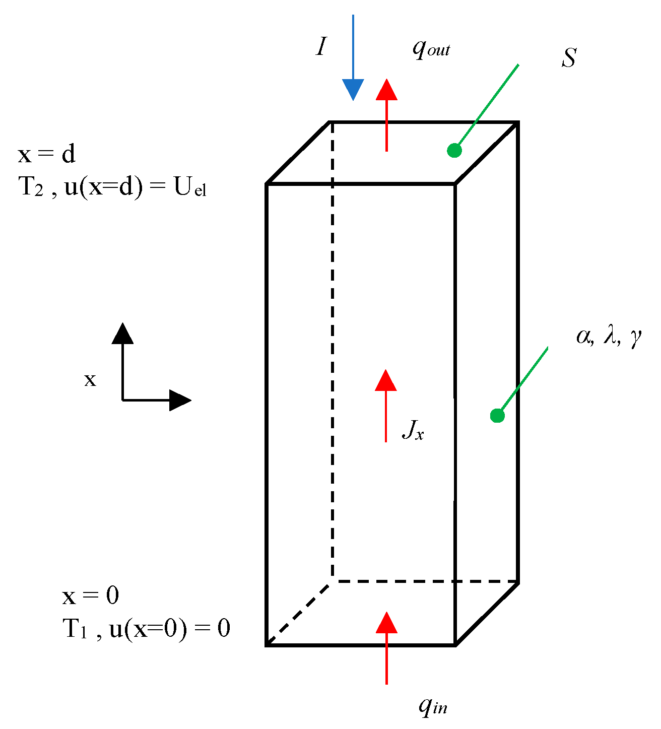
where (A·m−2) is the current density vector, (W·m−2) is the thermal flux density vector, ϕ (V) is the electric field potential, T (K) is the temperature, γ (S·m−1) is the electrical conductivity coefficient, λ (W·m−1 K−1) is the thermal conductivity coefficient, and α (V∙K−1) is the Seebeck coefficient. Additionally, ∇ (m−1) represents the Hamiltonian operator. Figure 1. shows the simplest possible arrangement:
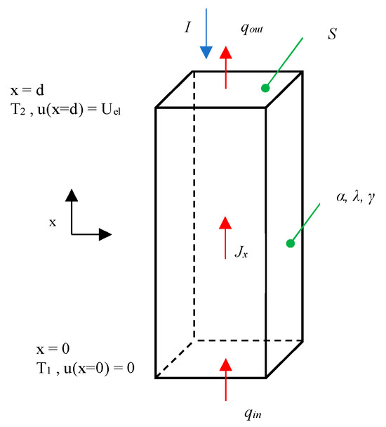
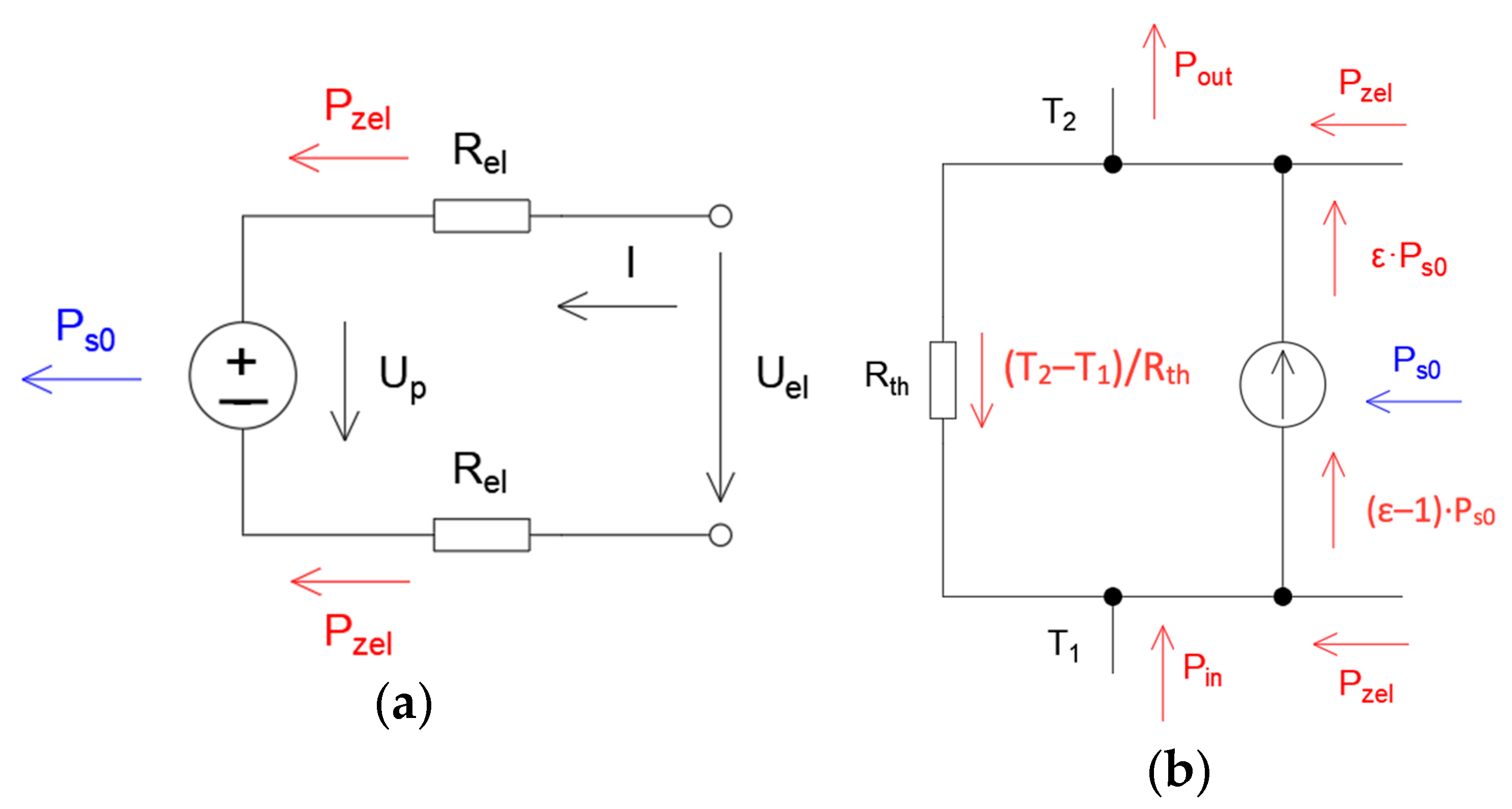
Figure 1.
The mathematical model of the considered TE module corresponds to the following simple scheme. The symbols shown correspond to the equations given.
The input parameter in this case is the current density vector. Assuming a steady state and ∂T/∂t = 0, the validity of the conservation of electric charge, we can consider the current density vector to be constant throughout the entire volume element of the substitute model. For the vector of electric field intensity in individual Cartesian coordinates, E = −∇ϕ, (Ex, Ey, Ez) must hold. Assuming propagation only in the x-axis direction (Ex, 0, 0), the equation can be rewritten as follows:
where u (V) is the electric voltage. To define the current density vector, we start from Ohm’s law in its differential form, denoted as = γ∙.
Ex = −dϕ/dx = −du/dx
For this vector, in Cartesian coordinates, it must also satisfy = (Jx, Jy, Jz); when considering propagation only in the x-axis direction, it follows = (Jx, 0, 0). The resulting current density vector in the x-axis is:
Jx = γ·Ex = −γ·du/dx
Let us now start from the thermal Fourier Kirchhoff equation in the form [30]:
where ρ (kg·m−3) is the density, cp (J·kg·K−1) is the specific heat capacity at constant volume V = const., and (m·s−1) is the velocity vector. Assuming propagation only in the x-axis direction, the heat flux vector takes the form = (qx, qy, qz) = (qx, 0, 0). The steady-state condition ∂T/∂t = 0 still holds. We chose the reference coordinate system in Cartesian coordinates with respect to the TE module, which is stationary, meaning the velocity of the medium is = 0 (m·s−1). The resulting form of the Fourier Kirchhoff equation in the considered x-axis is:
0 = −d·qx/dx − Jx ·du/dx
After substitution and adjustments, we obtain a system of two differential equations. The first equation is a second-order thermal differential equation in the form:
0 = −Jx·α·dT/dx − Jx·du/dx+ λ·d2T/d2x
As the second equation, we obtain a first-order electrical differential equation:
Jx = −γ·du/dx − γ·α·dT/dx
With the initial conditions for this system of differential equations being T (x = 0) = T1, T (x = d) = T2, u (x = 0) = 0, solving these two differential equations with the corresponding initial conditions and subsequent adjustments leads to the following three equations:
where d (m) is the length of the element and Uel (V) is the applied voltage across the element. Assuming that the volume in each part is homogeneous, we can proceed to a model with concentrated parameters:
where I (A) is the total electric current flowing through the element. When considering the directional sign convention for consumers, the positive product of power flow into the system must hold, i.e., I·u(d) = I·Uel. Furthermore, we define the electrical resistance of the element Rel (Ω) by the equation:
qin = Jx·T1·α − d·J2x/2γ + (T1 − T2)·⅄/d
qout = Jx·T2·α − d·J2x/2γ + (T1 − T2)·⅄/d
u (d) = Uel = α·(T1 − T2) − d·jx/γ
Jx = I/S
Rel = d/(2·γ·S)
In addition, the thermal resistance of the element (bypass thermal resistance) Rth (kW−1) is defined as:
where S (m2) is the area of the element, Rel (Ω) is the resistance of the element, and Rth (kW−1) is the thermal resistance of the element.
Rth = d/(⅄·S)
Moreover, we can represent the thermoelectric voltage Up (V) using the following equation:
Up = α·(T2 − T1)
After substituting, the total electric voltage Uel (V) can be expressed as:
Uel = Up + 2·Rel·I
This equation is representative of the modified electrical diagram illustrated in Figure 2b.
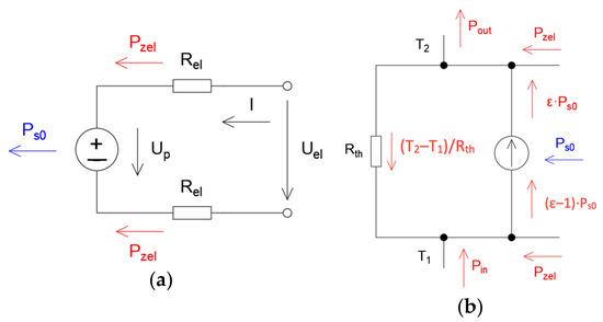
Figure 2.
The substituted electrical (a,b) thermal diagram of a single TE module in the considered model. Substituted diagrams (a,b) correspond to the stated equations, as do all symbols.
For thermal Joule losses Pzel (W) in ohmic resistances, the following equation holds:
Pzel = Rel·I2
It is true that the equal distribution of Joule losses between the ends of the junctions is valid only for constant thermal and electrical conductivity of the material. We assumed that (according to “www.thermonamic.com.cn (accessed on 13 August 2024)”) in the case of the BiTe3 material, the electrical conductivities P and N material differ by approximately ten percent and the thermal conductivities by approximately three percent, and they are also thermally dependent. It turned out that there is no analytical solution of differential equations in a closed finite form when considering analytical interpolations of temperature dependences of electrical and thermal conductivity, and finding the parameters of a discrete model is not possible. Instead of solving algebraic equations, the correct solution would mean optimization over the solution of systems of differential equations, but the time required for the calculations is, of course, very much higher. So, we were satisfied with the usual procedure and, as in the cited literature, we divided the Joule losses equally between the ends.
In addition, the nonentropic electric power PS0 (W) supplied by the voltage source is given by:
PS0 = Up·I = α·(T2 − T1)·I
To construct the thermal equivalent circuit, it will first be necessary to define the input power Pin (W) and the output power Pout (W):
Pin = S·qin
Pout = S·qout
The substitute thermal diagram describing the system is depicted in Figure 2b: After adjusting the equations for qin and qout and considering the efficiency of the heat engine as a heating factor in the form of ε = ξCarnot T2/(T2 − T1), where 0 < ξCarnot < 1, we obtain the equations describing the substitute thermal diagram:
Pout + (T2 − T1)/Rth = Pzel + ε Ps0
Pin + Pzel − (T2 − T1)/Rth (ε − 1) Ps0
3. Model of Series Connection of Peltier Cells and Considered Parameters of Individual Layers
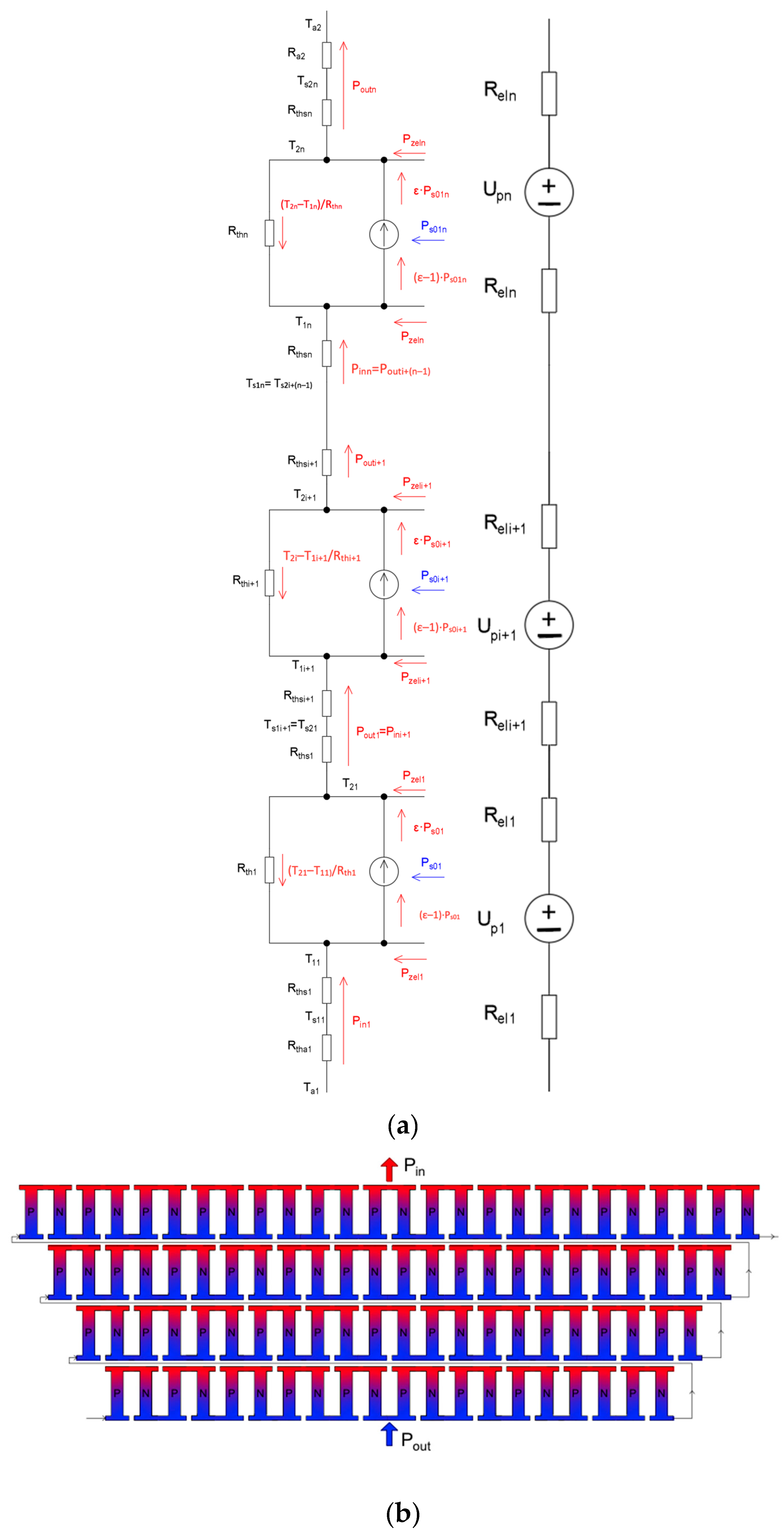
For the analysis of the behavior of TE modules connected in series, we built upon the previously derived model of a single TE module. Figure 3a depicts the substitute thermal electrical circuit of the connected TE modules. In each layer, the TE modules are connected electrically in series and thermally in parallel. These layers are subsequently connected thermally and electrically in series, forming a single long chain, whereas Figure 3b illustrates the possible configurations of multiple layers of TE modules as follows:
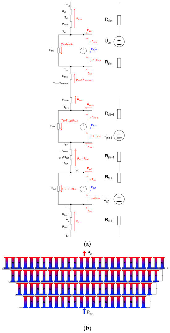
Figure 3.
(a) The substitute thermal and electrical diagram of the single TE module connected in series with general n TE modules. (b) Conceptual diagram showing the connections of multiple layers of TE modules.
For the given connection of n-layers of TE modules, the following equations must also hold:
Pouti + (T2i − T1i)/Rthi = Pzeli + εi·Ps0i
Pini + Pzeli + (T2i − T1i)/Rthi = (εi − 1)·Ps0i
εi = T2i/(T2i − T1i)
Pini = (Ts1i − T1i)/Rthsi
Pouti = (T2i − Ts2i)/Rthsi
PS0i = Upi·I = α·(Ti2 − T1i)·I
Pzeli = Reli ·I2
Since we are building on the model of a single TE module for series-connected TE modules, it is logical for their substitute diagrams and equations to be similar. In the model, we need to consider the influence of thermal resistances between the individual layers of TE modules, which are denoted here as Rthsi (kW−1). Furthermore, we assume the conservation of thermal powers Pout,i = Pin,i+1, the continuity of temperatures Ts2,i = Ts1,i+1, and that the same current flows through all the TE modules. To create a complete and unambiguous description of the model, we also need to define the thermal powers that enter and exit the system. We derive them from the known temperatures of the surrounding environment between which heat transfer occurs and from the knowledge of thermal resistances between TE modules and their surroundings. The equations for the input and output thermal power complement the model of the series connection of n layers of TE modules:
Pin,1 = (Ta,i − Ts1,1)/Rtha,1
Pout,n = (Ts2,n − Ta,2)/Rtha,2
When we examine how a TE module, as a physical electronic component, is actually designed, we find that it is composed of individual “elementary” TE modules [31]. We will refer to these “elementary” TE modules as eTE modules. In terms of electrical current, these eTE modules are connected in series, while in terms of heat transfer, the eTE modules operate in parallel. Let us denote the number of elementary cells in the i-th layer as neTEi. Then, we can formulate the following equations for the thermal and electrical properties of this layer:
Rth,i/Rth,1= neTEi/neTEi,1
Rel,i/Rel,1 = neTEi,i/neTEi,1
Up,i/Up1 = (neTEi,i/neTEi,1)·((T2,I − T1,i)/(T21 − T11))
The thermal resistances Rths,i between the individual layers of eTE modules are influenced by the structural design. For the sake of simplicity in our modeling, we assume that the cells are made of the same material. Therefore, we can estimate the values of Rths,i as:
Rths,i/Rths,1 = neTEi/neTE1
4. Optimization of the Operation of Series-Connected Peltier Cells
If we want to perform optimization, it can be intuitively assumed that a wrong approach would be to randomly choose values characterizing the parameters of the layers and the current passing through. It would be naive to think that randomly chosen layer parameters and current values would lead to effective operation of the resulting device. From a logical standpoint, it is evident that the value of Rths,i should be as small as possible to limit the backflow of heat through Rth. Achieving a low Rths,i is not a problem because the electrical voltage between the layers is small, and a thin layer for electrical insulation is sufficient. Additionally, it can be made from a material with good thermal conductivity.
For optimization, the absolute number of neTE1 is not essential. We chose the value neTE1 = 100. The actual optimization involves both integer optimization, which means finding values for neTEi pro i = 2, 3, … and continuous optimization, which means finding optimal current values I for the optimal values of neTEi. These values are chosen in such a way that the heating factor or coefficient of performance (COP,ε) of the system is maximized. Therefore, we are looking for the maximum of the expression:
εn = Pout,n/(I · ∑nj=1 Uelj) = Pout,n/(Pout,n − Pin1)
The results are shown numerically in Table 1. In the first column are the numbers of neTEi in the layers, in the second column the COP, and in the third the output power in the optimized state; the last column indicates the material mass relative to the state with a single layer with neTEi = 100. The increase in material mass (we consider the junction material as the most expensive component) is considerable, which is due to the fact that there are more neTEi in more layers, but also because, to achieve the specified output power, it is necessary to increase the number of neTEi in the layers in proportion to the lower output power in an optimized state with multiple layers.

Table 1.
The table shows the relative material costs of the multilayer TE module. The table also shows the optimized number of neTEi modules in each layer for the multilayer TE module, including the resulting coefficient of performance COP and output power Pout.
5. Parameter Identification for a Specific Peltier Cell
To utilize the resulting substitute model to simulate the actual behavior of the TE module, it is necessary to perform parameter identification. The search parameters are the values of Rtha1 = Rtha2 = 2 Rtha, Rth, and the Seebeck coefficient α [32]. To obtain these values, measurements were carried out on a fabricated device consisting of a single piece of TE module connected via thermal paste to two aluminum heat sink blocks labeled Al1 and Al2. These blocks are considered to have such good thermal conductivity that we can assume their temperature to be constant throughout their volume. The constructed product was eventually placed in a box and thermally insulated using assembly foam. The described experiment and its production can be seen in Figure 4b. Therefore, we treat the system as having concentrated parameters (a “lumped heat capacity system”). If temperature sensors are attached to these aluminum blocks, the surface temperature can be measured quite accurately. The time profiles of connected or generated voltage and current can be measured using an oscilloscope at the input terminals. The temperature measurement system (resistive sensors with electronics) was calibrated in the laboratory with an accuracy of 0.2 K, and the electrical resistance was measured by the four-wire method when passing alternating current with an uncertainty of 0.05 Ω. Uncertainties of thermal resistances were not determined, as it is a very complex task (time courses are filtered, then the data are fitted with exponential dependences, and values are determined from them). The authors were satisfied with the visual agreement of the measured and simulated waveforms with the obtained parameters and the approximate agreement with the values obtained from the datasheet. It was essential to make sure that the parameters were not fundamentally wrong. The described measuring setup and real implementation Figure 4b corresponds to the conceptual diagrams of the experiment in Figure 4a. The thermal diagram of the experiment is shown in Figure 4c.
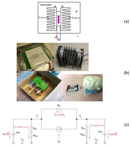
Figure 4.
(a) Conceptual diagram of apparatus with TE module. (b) Step-by-step demonstration of the real implementation of the experiment. (c) Substitute thermal diagram of the device.
In Figure 4c, m is the mass (kg), and c is the specific heat capacity (J·kg−1·K−1). The resistances Rtha1 a Rtha2 represent thermal resistance to the surroundings, and their values are mainly determined by the thermal resistance of the assembly foam, as it can be assumed that the thermal resistance of the heat sinks is significantly lower. A mounting PUR foam was used, for which the manufacturer indicated a coefficient of thermal conductivity 0.036 W/(m·K), and the resulting thermal resistances Rth1a and Rth2a had values of 46.7 kW−1; for the experiment, it is important that it is more than 37 times more than Rth. The disadvantage was that it was necessary to wait a relatively long time between experiments for the preparation to cool down. On the other hand, the values of m1c1 a m2c2 correspond to the thermal capacity and are mainly determined by the parameters of the respective heat sinks, as the thermal capacity of the assembly foam is very small. Therefore, it can be assumed that most of the heat will accumulate in these aluminum heat sinks.
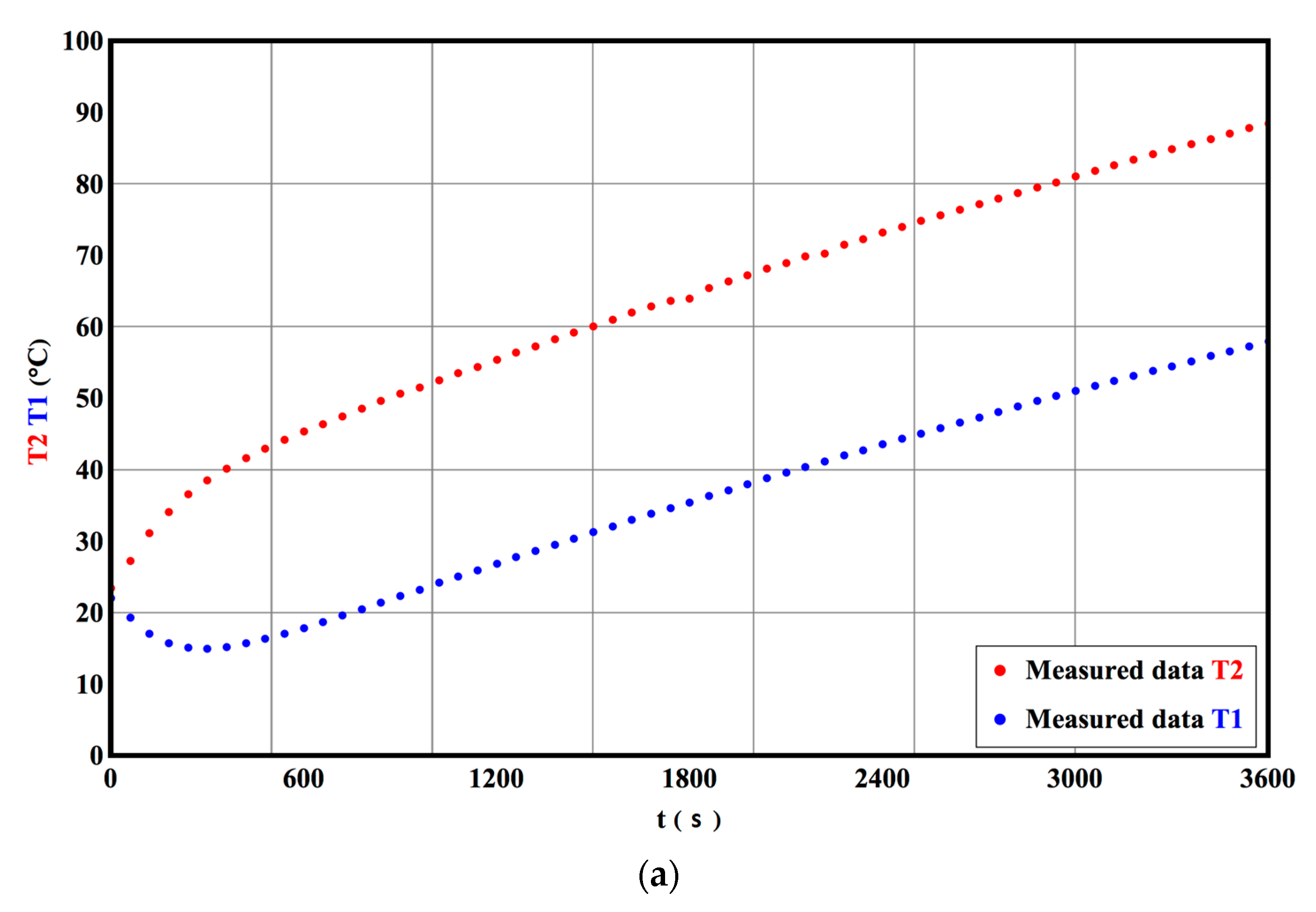
The ambient temperature was considered constant during the measurements. The profiles were measured as expected. After turning on (connecting the TE module to the power source; in our case, a stabilized power source with current limiting was used to behave as a constant current source), and after turning off, the profiles were obtained, as shown in Figure 5. The measured time courses after switching on are shown in Figure 5a. Initially, up to about 300 s, the heat engine first causes cooling on the cold side of the cooler Al1 and heating of the cooler Al2 on the hot side. However, as the temperature gradient on the TE module increases, the bypass thermal resistance Rth consumes a larger portion of the heat engine’s power. At a certain temperature gradient, its size stabilizes, and both temperatures then rise together because the thermal resistances to the surroundings, given by the properties of the insulating foam Rth1a and Rth2a, are relatively large. The situation after disconnection from the source is shown in Figure 5b. The behavior corresponds to the assumptions that the thermal resistance Rth is significantly lower than the thermal resistances Rth1a and Rth2a, and the temperatures T11 and T2n equalize before the heat sinks cool down together. It is essentially an analogy to the so-called regular phase method, where we assume exponential processes in the system with various time constants, one of which is the largest. Eventually, the body cools down to the point where it can be considered thermally homogeneous.

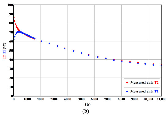
Figure 5.
Measured temperature dependences on the cold and hot sides of the heat sink for two situations, ambient temperature Ta = 24 °C. (a) After turning on. (b) After turning off.
We can consider the thermal resistances between the aluminum blocks and their surroundings to be the same due to their identical geometry. In the region where the temperatures of both blocks are essentially the same, the following holds:
where Rtha is the parallel combination of thermal resistances Rtha1 and Rtha2. We know the values of the product of mass and specific heat capacity quite precisely (weighing and material knowledge). The device was constructed in such a way that we can assume Rtha1 = Rtha2, which simplifies the evaluation of the measurements.
(m1 + m2)·c·dT/dt = (Ta − T)/Rtha
6. Determination of Peltier Module Parameters Based on Measured Data
To determine the parameters of the TE module and its surroundings, we will use the graphs from Figure 5b and Figure 6a, which can be divided into two regions: the cooling region of both sides of the TE module and the convergence of their temperatures to a common temperature. The second part corresponds to when a common temperature is reached on both sides of the TE module, and they subsequently cool together to the ambient temperature.
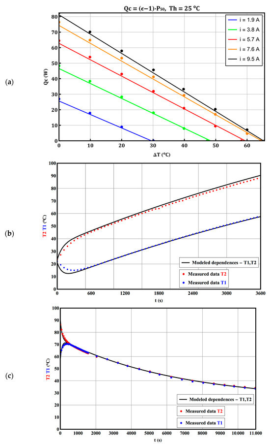
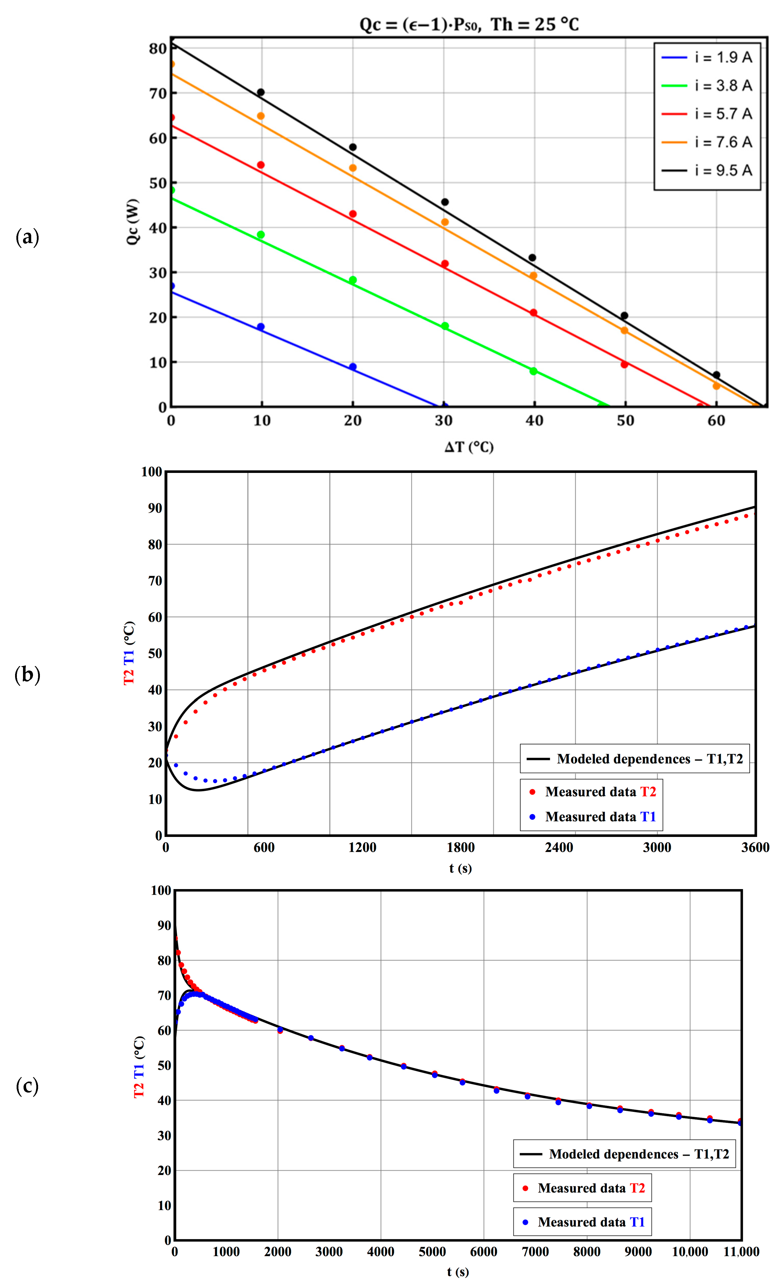
Figure 6.
(a) Cooling power profiles of the TE module as a function of the temperature difference between the cold and hot sides of the TE module. Comparison of temperature profiles on the cold and hot sides of heat sinks between measured data and modeled dependences. (b) After power-on. (c) After power-off. Ambient temperature Ta = 24 °C.
The value of Rtha will be determined using regression methods in the region where the temperatures on both sides of the TE module equalize, and during their simultaneous cooling. Additionally, we assume the same thermal resistance for heat transfer on both sides of the TE module, so it holds that Rtha1 = Rtha2 = 2Rtha.
We will determine the value of the bypass thermal resistance Rth from the region where the temperatures on both sides of the TE module are approaching each other, with knowledge of Rtha1, Rtha2, or Rtha from the previous step.
We will determine the value of the Seebeck coefficient α based on the measured temperature profiles in Figure 5b and the measured values of UP. Since UP = α (T2 − T1) holds when I = 0, regression analysis can be used to determine the coefficient α once again.
We can easily determine the value of Rel by measuring the resistance using the ohmic method with alternating current based on the measured profiles in Figure 5a. Alternating current, due to the Peltier effect, generates an opposite thermal gradient in the first half period compared to the second half period. Therefore, for measuring electrical resistance, it can be assumed that these effects cancel each other out, meaning that no thermoelectric voltage is generated. Additionally, aside from the Peltier effect, Joule losses need to be considered. However, these losses will heat both sides of the TE module equally, resulting in no temperature difference on either side of the TE module. The time constants of thermal processes are much larger than 0.02 s, corresponding to the grid frequency period. In the end, we can consider Up = α·ΔT where ΔT → 0 K, and thus Up → 0 V. This means that this countervoltage does not affect the value of the measured resistance.
7. Determination of Peltier Module Parameters Based on Manufacturer’s Datasheet Data
In the study [33], formulas for calculating the parameters α, Rel and Rth are derived. Similar formulas are used by other authors, for example, [31,32]. These formulas take into account the maximum values of thermal and electrical quantities that may appear in the TE module during nondestructive operation.
where TH corresponds to the hot-side temperature T2, and ΔT is the temperature difference T2 − T1. The manufacturer provides two sets of parameters in the datasheet, one for TH = 25 °C and another for TH = 50 °C.
α = Uel,max/TH
Rel = ((TH − ΔTmax)·Uel,max)/TH·Imax
Rth = (2TH·ΔTmax)/((TH − ΔTmax) · Uel,max·Imax)
The following table (see Table 2) presents the values of α, Rel and Rth obtained both by measurements and by using the manufacturer’s parameters, with their substitution into the formulas mentioned earlier. Based on this table (see Table 2), the calculated values from the measured data can be considered accurate. Therefore, they will be used for further modeling in case studies.
Table 2.
Comparison of α, Rel, and Rth values calculated using formulas and datasheet data and based on values obtained by measurement. The datasheet provides data for hot side temperatures of 25 °C and 50 °C.
8. Case Study
With the identified parameters of HP-127100 obtained from the described measurements, numerical experiments were carried out. The values obtained from the measurements on the test setup are:
Rtha1 = Rtha2 = 46.74 kW−1, Rth1 = 1.29 kW−1, Rel1 = 0.65 Ω
α = Up1/(T21 − T11) = 49.36 mVK−1, Ta = = 24 °C
The comparison of cooling power profiles of the TE module as a function of the temperature difference between the cold and hot sides of the TE module is displayed in Figure 6a. The data points from the manufacturer’s datasheet are shown as dots, and the solid lines represent the profiles of the model, utilizing calculated parameters from measured values. The graphs below show temperature profiles to verify the correctness of the measured data and the subsequently calculated TE module parameters. Here, solid lines represent the profiles obtained through modeling, and dots represent the measured data.
A comparison of the temperature profiles on the cold and hot sides during dynamic processes is shown in Figure 6, i.e., connecting the TE module to the power source in Figure 6b and disconnecting the TE module from the power source in Figure 6c.
Values selected for modeling multiple TE module layers:
Rtha1 = Rtha2 = 0.25 kW−1, Rths1 = 0.12 kW−1
Rth = 1.29 kW−1, α = Up1/(T21 − T11) = 49.36 mVK−1, Rel1= 0.65 Ω,
Ta1 = 10 °C, Ta2 = 27 °C
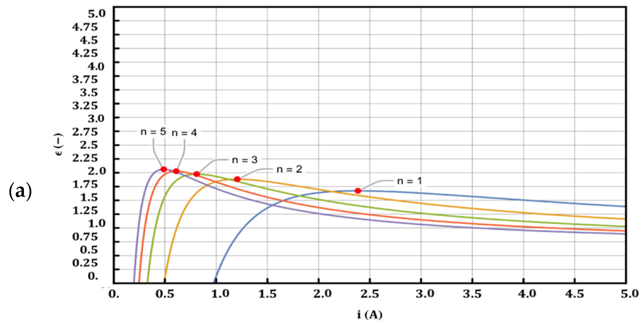
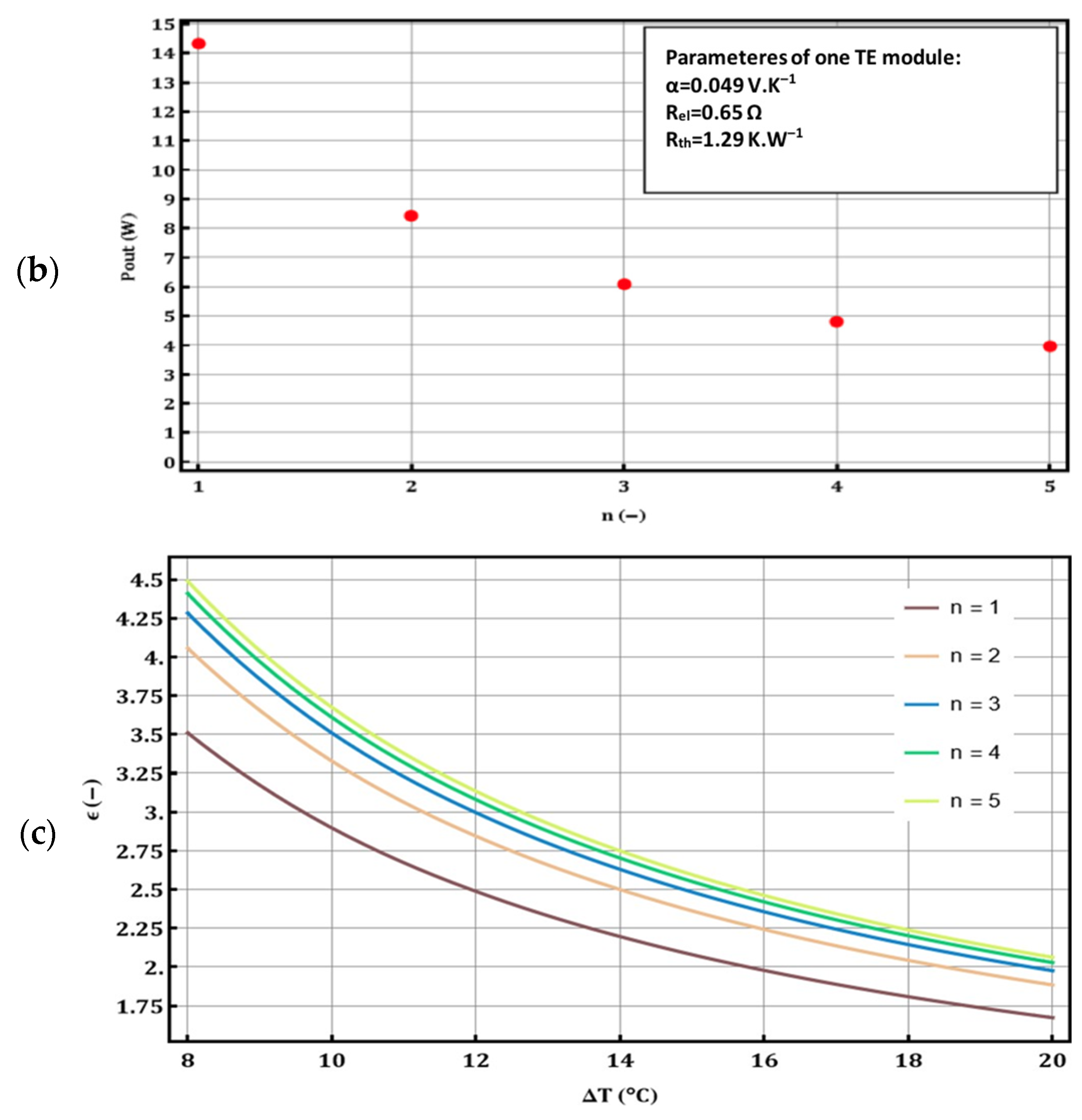
In Figure 7a, the dependence of ε (COP) on current is depicted for configurations of TE modules with layers ranging from 1 to 5. For each layer count, the point εmax (COPmax) is also marked in red, representing the current at which maximum ε is achieved. The trends show that optimal values of ε shift closer to lower current values with an increasing number of layers and exhibit a slight growth.

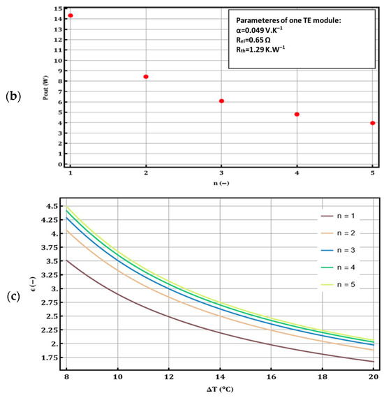
Figure 7.
(a) Dependence of ε on the electric current for the considered number of layers 1–5. Higher values of ε can be achieved with an increasing number of layers and a lower current. (b) Dependence of output power Pout on the number of layers. Despite achieving a higher ε, the actual output thermal power decreases. (c) Dependence of ε on temperature difference for 1–5 layers. In accordance with expectations, the lower the temperature difference, the higher the values the ε model attains. Additionally, it can be noted that, once again, ε increases with the growing number of layers. However, it is evident that the curves for layers n = 3, 4, 5 practically coincide, indicating that the increase in the ε value by adding layers 4 and 5 is relatively small compared to adding layers 2 and 3.
In Figure 7b, the output thermal powers at the optimal current for the investigated number of layers are displayed.
Looking at Figure 7a, we can see that higher values of ε can be achieved with lower currents as the number of layers increases. However, as shown in Figure 7b, despite achieving a higher ε, the actual output thermal power decreases.
In Figure 7c, the dependences of ε on the temperature difference between the input (Ta1) and output (Ta2) sides of the model composed of n layers are subsequently plotted.
9. Case Study Conclusions
By connecting multiple Peltier modules in series, we observed a significant improvement in the thermal pump’s ability to transfer heat from one environment to another. This allowed us to achieve higher temperature differentials and a more efficient heat transfer. Additionally, distributing the electrical load across multiple TE modules reduces the burden on individual TE modules, thereby increasing the lifespan and reliability of the entire system.
As part of the study, the parameters of an actual TE module were measured and compared to theoretically calculated parameters (see Table 2), which were computed using commonly used formulas, such as those from [34]. The parameters derived from the measurements matched the theoretically calculated parameters, validating their accuracy. Using these measurement parameters, simulations of series–parallel structures with a larger number of TE modules were conducted.
Simulations were conducted to investigate the optimization of the coefficient of performance (COP) by employing an appropriate arrangement of a greater number of TE modules. The modeled structure consisted of n layers, which were thermally and electrically connected in series. Each layer contained a set of elementary TE modules (eTE modules) connected electrically in series and thermally in parallel.
The simulation results indicated that, for multiple layers, the maximum COP consistently trended toward lower current values. From an optimization standpoint regarding the number of layers, employing up to three layers makes sense, as further layer addition yields marginal overall COP growth, potentially rendering it suboptimal from an economic perspective, considering capital expenditures.
In conclusion, our study presents the possibility of employing a serial arrangement of Peltier modules as thermal pumps. Leveraging the increased performance and improved energy utilization afforded by these configurations has the potential to enhance heat transfer efficiency and effectiveness in various applications. Further research in this domain, including the exploration of advanced control strategies and module designs, holds promise for future advancements in Peltier-based thermal systems.
As a conclusion for manufacturers, flexible technology is recommended for Peltier cells to be used as heat pumps (for example, for heating low-energy single-family houses). For specified T1s and T2s, or for specific heating systems in specified climatic locations, it is possible to find the optimal number of junctions in the individual layers of the pyramid arrangement. The thermal resistance between the layers should be as small as possible, and the inlet and outlet should be adapted for the installation of heat supply and removal, for example, using heated tubes.
The model is, of course, not new, but perhaps the use of optimization algorithms can be considered an interesting new fact, i.e., that the number of junctions in the individual layers must be optimized simultaneously with the supply current to obtain the best and transferred thermal power and subsequently the best total size of the device, if the input is specified as input or output power with temperatures T1 and T2 and maximum COP is required.
Optimization and all calculations were performed in SW Wolfram Mathematica. The optimization procedure consisted of several steps. First, a function was created that takes as input a tuple of numbers—that is, the number of neTEi in the layers and the supply electric current—and returns the COP. This function was used in another function that has an input of a tuple of numbers (i.e., the number of neTEi in the layers), and returns the value of the supply current at which the COP is maximal and the corresponding COP. Since, for the given tuple, neTEi COP is a continuous smooth function of the current that has a local maximum, the search for the maximum using the gradient method implemented in SW was used. Discrete optimization of this function was then used, where neTEi values were searched for n > 1. This function uses the NMaximize function, which allows one to enter the region from which the searched variables can be extracted. In our case, it turned out to be sufficient to limit oneself to integers between 90 and 150. The optimality of the results was tested by calculating the COP values for integers adjacent to the optimization result. The authors consider this optimization approach to be original. Regarding the production of equipment, if it were to be shown that it is possible to use layered structures for heating low-energy family houses, it would be necessary to design the heating system as a whole. According to the authors, it would be advisable to connect the layered structures with heat exchangers through heat pipes. However, it would be necessary to recruit experts from other technical fields to design such systems.
Author Contributions
J.R. participated in reviewing the literature related to the study, conducted the experiments and collecting results, compiled the data, wrote results, and wrote the first draft. J.K. (Jan Kyncl) provided supervision on the project and reviewed the manuscript. J.K. (Jan Koller) is the principal investigator for the project, initiating the conceptualization and supervising. G.F. is the co-supervisor of the project and assists with research development. All authors have read and agreed to the published version of the manuscript.
Funding
SGS23/167/OHK3/3T/13, Czech Technical University in Prague.
Data Availability Statement
Data are contained within the article.
Conflicts of Interest
The authors declare no conflicts of interest.
References
- Sun, Y.; Liu, Y.; Li, R.; Li, Y.; Bai, S. Strategies to Improve the Thermoelectric Figure of Merit in Thermoelectric Functional Materials. Front. Chem. 2022, 10, 865281. [Google Scholar] [CrossRef] [PubMed]
- Chen, L.; Yu, Z.; Yuan, Y.; Zhang, J.; Lee, J. Electrical performance optimization of a transverse-Seebeck-effect-based tubular thermoelectric generator for waste heat recovery. Energy Rep. 2022, 8, 7589–7599. [Google Scholar] [CrossRef]
- Riffat, S.B.; Ma, X. Improving the coefficient of performance of thermoelectric cooling systems: A review. Int. J. Energy Res. 2004, 28, 753–768. [Google Scholar] [CrossRef]
- Renge, S.; Barhaiya, Y.; Pant, S.; Sharma, S. A Review on Generation of Electricity using Peltier Module. Int. J. Eng. Res. 2017, V6, 453–457. [Google Scholar] [CrossRef]
- Zhu, K.; Bai, S.; Kim, H.S.; Liu, W. Module-level design and characterization of thermoelectric power generator. Chin. Phys. B 2022, 31, 048502. [Google Scholar] [CrossRef]
- Luo, D.; Wang, R.; Yu, W.; Zhou, W. Parametric study of a thermoelectric module used for both power generation and cooling. Renew. Energy 2020, 154, 542–552. [Google Scholar] [CrossRef]
- Sandoz-Rosado, E.; Stevens, R. Robust Finite Element Model for the Design of Thermoelectric Modules. J. Electron. Mater. 2010, 39, 1848–1855. [Google Scholar] [CrossRef]
- Ge, Y.; He, K.; Xiao, L.; Yuan, W.; Huang, S.-M. Geometric optimization for the thermoelectric generator with variable cross-section legs by coupling finite element method and optimization algorithm. Renew. Energy 2021, 183, 294–303. [Google Scholar] [CrossRef]
- Tohidi, F.; Holagh, S.G.; Chitsaz, A. Thermoelectric Generators: A comprehensive review of characteristics and applications. Appl. Therm. Eng. 2021, 201, 117793. [Google Scholar] [CrossRef]
- Huang, G.-Y.; Hsu, C.-T.; Fang, C.-J.; Yao, D.-J. Optimization of a waste heat recovery system with thermoelectric generators by three-dimensional thermal resistance analysis. Energy Convers. Manag. 2016, 126, 581–594. [Google Scholar] [CrossRef]
- Zhang, J.; Zhao, H.; Feng, B.; Song, X.; Zhang, X.; Zhang, R. Numerical simulations and optimized design on the performance and thermal stress of a thermoelectric cooler. Int. J. Refrig. 2023, 146, 314–326. [Google Scholar] [CrossRef]
- Afshari, F. Experimental Study for Comparing Heating and Cooling Performance of Thermoelectric Peltier. J. Polytech. 2020, 23, 889–894. [Google Scholar] [CrossRef]
- Yin, T.; He, Z.-Z. Analytical model-based optimization of the thermoelectric cooler with temperature-dependent materials under different operating conditions. Appl. Energy 2021, 299, 117340. [Google Scholar] [CrossRef]
- Trancossi, M.; Kay, J.; Cannistraro, M. Peltier cells based acclimatization system for a container passive building. Tec. Ital. J. Eng. Sci. 2018, 61, 90–96. [Google Scholar] [CrossRef]
- Cai, Y.; Huang, X.-Y.; He, J.-W.; Huang, Y.-X.; Zhao, F.-Y. Investigation of thermoelectric ventilated building envelope for simultaneously passive cooling and energy savings: Critical analysis and parametric characteristics. Energy Build. 2023, 297, 113421. [Google Scholar] [CrossRef]
- Rittner, E.S. On the Theory of the Peltier Heat Pump. J. Appl. Phys. 1959, 30, 702–707. [Google Scholar] [CrossRef]
- Maryani, S.; Kusumanto, R.; Rs, C. Solar Panel Optimization Using Peltier Module TEC1-12706. J. Mech. Civ. Ind. Eng. 2023, 4, 43–50. [Google Scholar] [CrossRef]
- Ficker, T. Simplified Peltier heat pump. Eur. J. Phys. 2022, 43, 045102. [Google Scholar] [CrossRef]
- Ibañez-Puy, M.; Bermejo-Busto, J.; Martín-Gómez, C.; Vidaurre-Arbizu, M.; Sacristán-Fernández, J.A. Thermoelectric cooling heating unit performance under real conditions. Appl. Energy 2017, 200, 303–314. [Google Scholar] [CrossRef]
- Barako, M.T.; Park, W.; Marconnet, A.M.; Asheghi, M.; Goodson, K.E. Thermal Cycling, Mechanical Degradation, and the Effective Figure of Merit of a Thermoelectric Module. J. Electron. Mater. 2012, 42, 372–381. [Google Scholar] [CrossRef]
- Barako, M.T.; Park, W.; Marconnet, A.M.; Asheghi, M.; Goodson, K.E. A reliability study with infrared imaging of thermoelectric modules under thermal cycling. In Proceedings of the 13th IEEE Intersociety Conference on Thermal and Thermomechanical Phenomena in Electronic Systems (ITherm), Orlando, FL, USA, 30 May–2 June 2012; pp. 86–92. [Google Scholar]
- Sun, Y.; Meng, F.; San, B.; Xu, C. Performance Analysis of Multistage Thermoelectric Cooler with Water-Cooled. J. Phys. Conf. Ser. 2023, 2442, 12028. [Google Scholar] [CrossRef]
- Karimi, G.; Culham, J.; Kazerouni, V. Performance analysis of multi-stage thermoelectric coolers. Int. J. Refrig. 2011, 34, 2129–2135. [Google Scholar] [CrossRef]
- Hwang, G.; Gross, A.; Kim, H.; Lee, S.; Ghafouri, N.; Huang, B.; Lawrence, C.; Uher, C.; Najafi, K.; Kaviany, M. Micro thermoelectric cooler: Planar multistage. Int. J. Heat Mass Transf. 2009, 52, 1843–1852. [Google Scholar] [CrossRef]
- Bergman, T.L.; Incropera, F.P. Introduction to Heat Transfer, 6th ed.; John Wiley & Sons: Hoboken, NJ, USA, 2011; ISBN 9780470501962. [Google Scholar]
- Petkov, T.; Belovski, I.; Ivanov, K.; Aleksandrov, A. Modeling the Parameters of a Cascaded Peltier Module using Neural Network. In Proceedings of the 21st International Symposium on Electrical Apparatus & Technologies (SIELA), Bourgas, Bulgaria, 3–6 June 2020; pp. 1–4. [Google Scholar]
- Wang, Y.T.; Liu, W.; Fan, A.W.; Li, P. Performance Comparison between Series-Connected and Parallel-Connected Thermoelectric Generator Systems. Appl. Mech. Mater. 2013, 325-326, 327–331. [Google Scholar] [CrossRef]
- Ivanov, K.; Belovski, I.; Aleksandrov, A. Study of Multi-stage Peltier Module in Generator Mode. In Proceedings of the 7th International Conference on Energy Efficiency and Agricultural Engineering (EE&AE), Ruse, Bulgaria, 12–14 November 2020; pp. 1–4. [Google Scholar]
- Fan, X.; Sun, H.; Yuan, Z.; Li, Z.; Shi, R.; Razmjooy, N. Multi-objective optimization for the proper selection of the best heat pump technology in a fuel cell-heat pump micro-CHP system. Energy Rep. 2020, 6, 325–335. [Google Scholar] [CrossRef]
- Lucas, S.; Bari, S.; Marian, R.; Lucas, M.; Chahl, J. Cooling by Peltier effect and active control systems to thermally manage operating temperatures of electrical Machines (Motors and Generators). Therm. Sci. Eng. Prog. 2022, 27, 100990. [Google Scholar] [CrossRef]
- Lineykin, S.; Ben-Yaakov, S. Analysis of Thermoelectric Coolers by a Spice-Compatible Equivalent-Circuit Model. IEEE Power Electron. Lett. 2005, 3, 63–66. [Google Scholar] [CrossRef]
- Zhang, H.; Mui, Y.; Tarin, M. Analysis of thermoelectric cooler performance for high power electronic packages. Appl. Therm. Eng. 2010, 30, 561–568. [Google Scholar] [CrossRef]
- Tozaki, K.-I.; Sou, K. Novel Determination of Peltier Coefficient, Seebeck Coefficient and Thermal Resistance of Thermoelectric Module. Jpn. J. Appl. Phys. 2006, 45, 5272. [Google Scholar] [CrossRef]
- Arora, R.; Kaushik, S.; Arora, R. Multi-objective and multi-parameter optimization of two-stage thermoelectric generator in electrically series and parallel configurations through NSGA-II. Energy 2015, 91, 242–254. [Google Scholar] [CrossRef]


Disclaimer/Publisher’s Note: The statements, opinions and data contained in all publications are solely those of the individual author(s) and contributor(s) and not of MDPI and/or the editor(s). MDPI and/or the editor(s) disclaim responsibility for any injury to people or property resulting from any ideas, methods, instructions or products referred to in the content. |
© 2024 by the authors. Licensee MDPI, Basel, Switzerland. This article is an open access article distributed under the terms and conditions of the Creative Commons Attribution (CC BY) license (https://creativecommons.org/licenses/by/4.0/).