A Non-Intrusive Load Decomposition Model Based on Multiple Electrical Parameters to Point

Abstract

The sliding window method is commonly used for non-intrusive load disaggregation. However, it is difficult to choose the appropriate window size, and the disaggregation effect is poor in low-frequency industrial environments. To better handle low-frequency industrial load data, in this paper, we propose a vertical non-intrusive load disaggregation model that is different from the sliding window method. By training multiple electrical parameters at a single point on the bus end with the corresponding load data at the branch end, the proposed method, called multiple electrical parameters to point (Mep2point), takes the electrical parameter data sampled at a single point on the bus end as its input and outputs the load data of the target device sampled at the corresponding point. First, the electrical parameters of the bus end are processed, and each item is normalized to the range from 0–1. Then, the electrical parameters are vertically arranged by their time point, and a convolutional neural network (CNN) is used to train the model. The proposed method is analyzed on low-frequency industrial user data sampled at a frequency of 1/120 Hz in the real world. We compare our method with three advanced sliding window methods, achieving an average improvement ranging from 9.23% to 22.51% in evaluation metrics, while showing substantial superiority in the actual decomposed images. Compared with three classical machine learning algorithms, our model, using the same amount of data, significantly outperforms these methods. Finally, we also compared our method with the multi-channel low window sequence-to-point (MLSP) method, which also selects multiple electrical parameters. Our model’s complexity is much less than that of the MLSP model, and its performance remains high. The superiority of our model, as presented in this paper, is fully verified by experimental analysis, which can produce better actual load decomposition results from each branch and contribute to the analysis and monitoring of loads in industrial environments.

1. Introduction

Technological advancements are occurring at an unprecedented rate, propelling the global economy to new heights. At the core of all these developments lies energy, which serves as the foundation for progress [1]. Considerable energy is wasted in traditional power systems. Against the background of energy savings and environmental protection, the efficient management and effective utilization of electric power energy have become the focus of research on electric power [2]. As the most basic part of power energy management, load monitoring has also become a key topic. Intrusive load monitoring technology can clearly, stably, and correctly obtain detailed power information by extracting and analyzing the power load information of each installed power monitoring device. However, this method also has a natural problem. The costs of installing, deploying, and maintaining this method are complex and expensive, and it is difficult to use in practice [3]. In 1985, Hart et al. [4] proposed a non-intrusive load decomposition technology that can read information from the bus end to analyze the load operation of the corresponding branch. Non-intrusive load monitoring (NILM) methods are simple to deploy and install, have low hardware costs, and have broad application prospects [5].

At present, researchers mainly focus on family houses, and a lack of in-depth research has been conducted on the non-invasive decomposition and identification of high-energy industrial loads [6]. According to an analysis of power consumption data released by China Electric City, the domestic electricity consumption of urban and rural residents accounts for only approximately 15% of the total social electricity consumption level, while industrial electricity consumption accounts for more than 65% of the total. At the same time, the proportion of industrial power consumption in social power consumption is maintained at a high level [7]. Therefore, the extensive application of non-intrusive load decomposition technology in industrial environments is highly valuable for helping industrial users save energy and reduce production costs. In an industrial environment, the structure of load equipment is complex, and power loads are unique. Non-intrusive load decomposition technology faces great challenges in this field. In a residential environment, the load data of most equipment can be obtained in one day. In the morning, middle, and evening, microwave ovens, refrigerators, lights, air conditioners, and so on can be used as their one-day operation cycles. The low-frequency adoption intervals of common residential environmental load datasets are 1 s~10 s, for example, 3 s for the REDD dataset [8], 6 s for the UK-DALE dataset [9], and 8 s for the REFIT dataset [10].

An industrial environment is very different from a residential environment. On the one hand, industrial equipment, unlike household appliances, does not have complete operation cycles within a short period. On the other hand, industrial equipment, unlike residential appliances, does not have obvious timing characteristics and is more dependent on the production mode. In the real world, industrial equipment loads produce fewer events and need to be studied at a longer time scale. In addition, acquiring industrial load data is more difficult; the current digital level of industrial users is not high; large and small industrial users cannot acquire high-frequency industrial loads while ensuring high data acquisition quality; and the current data acquisition, communication, and storage capabilities cannot support the acquisition of such data at a higher frequency [11]. Therefore, it is more practical and valuable to study low-frequency load decomposition in industrial fields.

The sliding window method is necessary to address problems in the field of load decomposition, but for an industrial environment that is different from the corresponding home environment, the sliding window method used in load decomposition cannot effectively address low-frequency industrial loads with sampling intervals of several minutes. For residential devices with adoption frequencies of approximately 1 Hz, the selected window size has less influence on the results. However, for industrial workloads with intervals of several minutes, the impact of the window size on the results can be significant. At this frequency, the sliding window method fails to balance the contradiction between the window size and the time span.

In conclusion, within the domain of NILM, despite the broad application of the sliding window technique, it encounters restrictions in low-frequency industrial settings. At low frequencies, the quantity of input data within a sensible window size is insufficient to offer adequate features for learning. Opting to extend the window length results in an overextended time span, leading to even worse decomposition outcomes. To tackle this problem, the purpose of this research is to devise an innovative NILM model designed to address non-invasive load disaggregation tasks within low-frequency industrial contexts. The “Mep2point” model we propose takes multiple electrical parameters acquired at a specific time point on the bus side as input data and fits the power data at the corresponding branch at the same time point. This is a point-to-point learning method. Different from the common sliding window method, this method does not require a sliding window to decompose the bus, so it does not need to be restricted in terms of selecting a window. Through the analysis of various electrical parameters obtained at the bus end, the appropriate parameters are selected, and a deep neural network is introduced to decompose the load. First, a correlation analysis is carried out on various bus parameters, and their correlations are sorted from high to low. Then, the parameters with different correlations are selected for analysis to obtain the optimal parameter combination. Next, the selected parameters are input into the deep learning network for training to fit the branch load at the corresponding time point. Through an experimental verification involving actual industrial users, the proposed method is compared with the existing sliding window method. From the experimental results, it can be seen that the proposed method resolves some problems that the sliding window method cannot handle. The proposed method can better decompose low-frequency industrial equipment loads. The main contributions of this article are as follows:

• The correlations of the electrical parameters at the bus are analyzed, and the influences of various parameter combinations on the decomposition results are studied.
• We propose a multi-electrical parameter-to-point load decomposition method based on deep learning to address the low-frequency load data that the sliding window method cannot process.
• On a real-world low-frequency dataset, the optimal sliding window method is used as a benchmark, and the performance of the proposed model is evaluated by using multiple indicators. The superiority of the proposed method is verified.

The remainder of this article is organized as follows. In Section 2, we review the relevant research conducted in the field of industrial NILM. In Section 3, we analyze the proposed method. Section 4 contains detailed information about the utilized data, and we present the relevant results of the experiments. Finally, Section 5 summarizes this article.

2. Related Work

NILM, which was first proposed by Hart in 1992 [4], separates single power measurements acquired from a central meter to estimate the power usage levels of different loads. The total power consumption signal produced at time t can be expressed as:

$$X(t)={\displaystyle \sum _{i=1}^L{Y}_i(t)+g(t)}$$

(1)

where Y_i(t) is the power consumption signal of load i at time t, L is the number of loads, and g(t) is the interference signal at time t.

The non-intrusive load decomposition process can be expressed as follows:

$$f(X(t))=\left[Y_1(t),Y_2(t),\cdots ,Y_L(t)\right]$$

(2)

where f denotes the mapping function used for non-intrusive load decomposition.

Event-based NILM is a classification problem. By extracting the operation characteristics of different electrical appliances, a corresponding feature library is established, the occurrences of events are detected, and the relevant features are extracted when an event occurs. Finally, the feature quantity is compared with the established feature library of the examined device to realize equipment classification. To address the event-based NILM problem, we can extract features and then classify the associated current and voltage data using machine learning methods such as linear regression, support vector machines (SVMs), and decision trees. In [11], this paper expands and evaluates appliance load signatures based on a hybrid method that uses the features extracted, i.e., current (I), harmonic (H), active and reactive power (P, Q), and the geometry of the curve V–I. The researchers in [12] mapped the original VI trajectories of household appliances to binary images. A LeNet model trained on the MNIST dataset was used to extract depth features from the binary VI images. Then, the ReliefF algorithm was used to select the most important information from the deep features. Based on the obtained load features, a support vector machine was used to identify the different appliances. Nonevent-based NILM refers to the monitoring and analysis of the energy consumed by appliances when no specific event occurs. Based on a bus power sequence or other features, the power sequence of the target appliance can be directly predicted, or the possible combinations of activated appliances can be speculated to decompose the electrical equipment. For such problems, deep learning is needed to process complex current and voltage data and to implement more accurate load monitoring and decomposition mechanisms. This means that when an appliance is used normally without specific operations or events, the constructed NILM system can still detect and identify the energy consumption of each appliance by analyzing the electrical energy data. The typical operation model for home appliances is a hidden Markov model. In [13], household appliances were modeled by using hidden Markov models, and a solution for implementing non-invasive load monitoring built on piecewise-based integer quadratic constraint programming was developed to decompose the household power distribution at the appliance level. This process was effectively verified in REDD and AMPds [14]. With advances in computer technology, deep neural networks have proven to be promising approaches for addressing these problems. In [15], a neural network-based sequence-to-point method, where the input is the window of a power supply and the output is a single point of the target device, was proposed, and a convolutional neural network (CNN) was used to train the model. We apply our neural network approach to real-world home energy data and show that our approach achieves state-of-the-art performance, improving two standard error measures by 84% and 92%.

In NILM, shallow learning and deep learning are two common machine learning techniques [16]. Shallow learning refers to methods that use traditional machine learning algorithms for modeling and prediction. These traditional algorithms usually include linear regression, SVMs, decision trees, etc. [17]. In NILM scenarios, shallow learning can be applied to perform feature extraction, classification, and regression tasks on current and voltage data [18], and the ADuCM4050 microcontroller was used for data processing in [19]. After applying event detection, data extraction, and other monitoring techniques, an SVM algorithm can be used to set and resolve the boundary to complete the identification process. Deep learning refers to the process of implementing modeling and learning using artificial neural networks [20]. It is characterized by a neural network structure with multiple hidden layers, which can acquire complex feature representations by learning a large amount of data. In NILM, deep learning can be used to handle complex current and voltage data and more accurately perform load monitoring and decomposition. Recently, deep learning has been widely used in various fields of NILM. In recent years, various deep learning architectures, such as CNNs, recurrent neural networks (RNNs), autoencoders, and transfer learning methods, have been developed in the field of NILM. In [21], three neural network architectures were proposed for energy decomposition purposes. Subsequent works have further developed NN-based NILM models to attain improved performance. In [22], long short-term memory (LSTM) was used to classify electrical appliances according to a denoising autoencoder. The main research direction of this paper concerned the non-invasive load decomposition problem encountered in industrial environments. The electrical energy consumption level was monitored and analyzed when no specific event occurred. Directly predicting a power sequence based on a bus power sequence or other features is a complex task, and the power sequences of industrial loads are very intricate. Machine learning methods such as SVMs and decision trees are very difficult to use. Therefore, deep learning is needed to solve this problem.

According to the application environment, NILM can be divided into residential, commercial, and industrial scenarios. Residential environments are currently the most widely studied settings in the field of NILM. In recent years, research on NILM in commercial and industrial environments has also increased. In a residential environment, NILM can monitor the energy consumption levels of different appliances in real time by monitoring their current and voltage data. By processing and analyzing these data, the energy consumption information of each appliance can be obtained, and the state of each appliance, such as its switching state and working mode, can be inferred. This can help residents understand the usage of individual appliances to formulate energy-saving strategies or to detect abnormal behaviors. At present, most NILM datasets, such as REDD, UK-DALE, AMPDS, REFIT, Dataport, ECO, BLUED, and PLAID, address residential environments. These scenarios have different sampling frequencies and different devices in rooms. In commercial environments, NILM can be applied to various types of places, such as office buildings, shopping malls, and hotels. By monitoring current and voltage data, the energy consumption information of each appliance or device can be obtained, decomposed, and analyzed. Commercial environments usually have complex energy requirements and diverse electrical equipment. NILM can help managers better understand information such as energy consumption distributions and peak and valley demands for energy management and optimization purposes. Regarding industrial environments, NILM can be applied in factories, production lines, and other places. By monitoring the current and voltage data of industrial equipment, the energy consumption of the equipment can be understood in real time and further decomposed and analyzed. This helps industrial enterprises address problems such as energy waste and equipment failures and take corresponding measures to improve energy utilization efficiency and production efficiency. With the global energy shortage, industrial environments account for more than 70% of the electricity consumption worldwide. Research on NILM in industrial settings is a future work direction. An industrial environment is different from a residential environment and a commercial environment; when transitioning from a residential environment to a commercial environment, most of the electrical appliances are similar but have different working states and time states. An industrial environment is very different from the current common residential environments. It has been difficult to address the problems concerning industrial environments with the previous methods and parameters.

In recent years, a multitude of studies have been conducted within the domain of non-intrusive load monitoring (NILM).

Table 1. Related work analysis table.

No.	Improvement Direction	Dataset	Method	Result	Year
1 [23]	An energy decomposition method based on real-time events. Enhancing the model’s real-time performance.	BLUED; Private dataset: Provided by NET2GRID BV, it includes aggregated active power measurements of selected appliances at a 100 Hz sampling rate from three households in the Netherlands, with data collected over a period of 15 days.	The model consists of three main parts: Event detection algorithm: Used to identify the instantaneous power changes when an appliance is turned on. Convolutional neural network (CNN) classifier: Used to recognize the transient response of specific target appliances. Power consumption estimation algorithm: Assumes a constant power consumption of the appliance and estimates the power consumption when a power drop is detected.	Experimental results show that for the three tested appliances (refrigerator, washing machine, and microwave oven), the system performs well in terms of real-time identification and power consumption estimation.	2021
2 [24]	An innovative multi-target energy disaggregation method capable of simultaneously decomposing multiple target devices.	UK-DALE; REFIT	The proposed model, named the variational multi-target regressor (V.M.Regressor), comprises the following main components: Variational encoder with convolutional layers. Multiple regression heads, which share parameters with the encoder. A combination mechanism for combining the outputs of the variational encoder. A shallow regressor network for estimating the power and on/off status of each target appliance.	Experimental results demonstrate that the proposed model excels in multi-target disaggregation tasks and is competitive when compared to existing multi-target and single-target models.	2023
3 [25]	Focused on low-frequency data, the model combines the spatial feature detection capability of CNN with the temporal data dependency capture capability of BiLSTM. It further optimizes the model’s focus on key parts of the data through the attention mechanism, enhancing the precision of event detection and load disaggregation.	The REDD dataset is used, with the sampling frequency reduced from 1 Hz to 0.1 Hz.	The model consists of three main parts: CNN: Used for classifying load types by leveraging spatial patterns in the data. BiLSTM: Processes sequential data and remembers long-term dependencies to capture complex temporal features in energy consumption data. Attention mechanism: Integrated into the BiLSTM model to enhance the model’s focus on key time steps in the input sequence, helping the model to more accurately identify the on/off patterns of appliances.	In terms of accuracy, the model’s classification accuracy is assessed using precision, recall, and the F1 score. The results show that the model has achieved excellent performance across all tested devices. In terms of computation time, the model demonstrates a significantly fast runtime, approximately 31 s and 19 milliseconds per step, which is crucial for timely load identification in real-time applications.	2024
4 [26]	A proactive learning framework was proposed that can learn and update a deep learning NILM model with a small amount of data, for transfer to a new environment.	REFIT	Deep learning model: A WaveNet-based NILM approach was used, creating separate models for each appliance to facilitate transfer learning. Active learning strategy: Strategies such as uncertainty sampling, batch BALD, and random sampling were employed to intelligently select samples that need to be labeled. Comparison between fine-tuning and full retraining: After each iteration of active learning, a comparison was made between using fine-tuning and fully retraining the model.	The experimental results in the paper demonstrate that the proposed active learning framework can significantly reduce the required labeling effort while maintaining accuracy. By using active learning, marking only 5–15% of the query pool data can achieve performance close to that of fully marking the entire query pool.	2023
5 [27]	The paper proposes a novel two-dimensional representation method that utilizes active (P) and reactive (Q) power data, which differs from traditional one-dimensional CNN architectures and better leverages the advantages of CNNs in processing two-dimensional data.	AMPds2, sampling frequency 1/60 Hz.	PQ signature representation: A two-dimensional representation method based on active and reactive power is proposed for creating 2-D PQ signatures. CNN regression: CNN models are used for regression analysis to estimate the power consumption of each device. The model includes PQ features in both the time and frequency domains.	The CNN model based on 2-D PQ signatures proposed in the paper performed exceptionally well on the AMPds2 dataset, achieving an estimation accuracy (EACC) of 96.1%, which represents an absolute improvement of 1.1% compared to previously reported methods on the same dataset.	2021
6 [28]	A new framework has been proposed, combining the multi-channel low sequence-to-point(MLSP) method with deep neural networks for load decomposition, in order to obtain more feature quantities from channels and address the issue of feature loss caused by small windows.	Private dataset: The actual industrial load dataset from a key distribution room of a large cement plant in China, with a sampling frequency of 1/300 Hz.	Multi-channel data fusion: A data fusion method has been proposed to aggregate multi-channel data on the same timeline, solving the problem of insufficient data features due to low sampling frequency. Deep neural network model: A deep learning model based on CNN has been designed to learn the features of data from the multi-channel low window sequence-to-point method and perform load decomposition.	The experimental results in the paper show that compared with the traditional Seq2point method, the proposed MLSP method has significantly improved across all evaluation metrics. When dealing with industrial loads that have complex fluctuation states, it can more accurately decompose the load fluctuations and more closely align with the actual load curve.	2024

provides an analytical overview of various research papers, offering a deeper insight into the content of several studies. The employment of deep learning methodologies for non-invasive load disaggregation has become a predominant research avenue. Athanasiadis and colleagues have realized real-time detection and power consumption estimation of target appliances by analyzing the aggregate data from a solitary monitoring vantage point. This was accomplished through the utilization of an event detection algorithm, a Convolutional Neural Network (CNN) classifier, and a power estimation algorithm. The experimental outcomes have demonstrated that the system excels not only in terms of real-time performance but also in computational and memory efficiency [23]. Virtsionis et al. [24] introduced a pioneering multi-target energy disaggregation approach that significantly enhances the precision of concurrent identification of energy usage across multiple appliances, employing a variational regression neural network. In the domain of NILM, challenges associated with low-frequency sampling have consistently been present, and the industrial settings investigated in this paper are characterized by an exceptionally low sampling frequency. Within the publication [25], Azzam and colleagues introduced an innovative hybrid learning approach that integrates CNN and bidirectional long short-term memory networks (BiLSTM), while also incorporating an attention mechanism to handle low-frequency power data. In [26], Todic and associates proposed a novel active learning framework designed to tackle the low-frequency NILM issue. This framework applies the principle of compressed sensing and combines it with deep learning models, effectively improving the performance of NILM algorithms under low sampling rate conditions. Continuously adding network modules can also increase the complexity of the model, which may lead to negative optimization of the results. In the industrial environment studied in this paper, situations with even lower sampling rates may be encountered, and a single input feature may struggle to learn the operation of devices at such a sampling scale. Some papers have improved the model’s decomposition capability by adding more input features. Schirmer and Mporas proposed an innovative NILM method that utilizes two-dimensional active and reactive signal features to enhance the accuracy of energy disaggregation. An estimation accuracy of up to 96.1% was achieved on a dataset with a sampling frequency of 1/60 Hz [27]. Therefore, not only can the active signal of the device be learned from the main bus signal, but also the decomposition accuracy can be improved by combining various electrical parameters of the main bus to increase the feature quantity. In the current low-frequency industrial environment, Meng Yang and others [28] proposed a multi-channel low window sequence-to-point (MLSP) method based on deep neural networks. This method fuses multi-channel bus data with the sequence-to-point model to expand the data volume within the same time window, thereby improving the model’s decomposition accuracy.

In summary, current research advancements have also focused on optimizing network models, adding network modules, or complicating simple features to increase input characteristics, thereby enhancing the model’s decomposition capabilities. Such approaches inevitably lead to a significant increase in model complexity, and most studies are based on optimizing the sliding window method. However, the size of the sliding window remains challenging to select, as different window sizes result in substantially varying output decomposition outcomes. For this purpose, this paper proposes a new NILM model: a non-invasive multi-electrical parameter-to-point load decomposition method. A sliding window does not need to be set, and the load decomposition process can be completed by fitting various electrical parameters corresponding to data acquired at the bus-end time point and the branch-end time point.

3. Multi-Electrical Parameter-to-Point Load Decomposition Method Based on a Deep Neural Network

It is difficult to obtain good decomposition results from the current advanced seq2point and seq2subseq methods in low-frequency industrial environments. Some hypotheses have been proposed to solve this problem. 1. The sliding window method has difficulty addressing low-frequency complex industrial data; therefore, the large sliding window framework should be removed. 2. Because many different electrical parameters are available at the bus end of the industrial dataset used in this paper, the branch load can be decomposed based on the information of various electrical parameters. 3. Different parameter combinations affect the decomposition results, and the parameters exhibiting greater correlations with the active power will be positively correlated with the results. Thus, the model framework and the experimental scheme of this paper are then constructed. The correlations among the parameters are analyzed, and the experimental group is arranged by the correlation values (from low to high). The final model of this paper is then constructed.

3.1. Electrical Appliance Parameter Analysis and Extraction

When addressing load decomposition problems, the sliding window method is inevitably used, and this method must select an appropriate window size. For high-frequency residential datasets, the window size has little impact on the results; examples include the low sampling frequencies of 1/3 Hz in the REDD dataset, 1/6 Hz in the UK-DALE dataset, and 1/8 Hz in the REFIT dataset [29]. The sliding window size is chosen from 299 to 599, and its corresponding timeline is 3–6 min. However, for load data acquired in industrial environments with low frequencies or even lower frequencies, the window size becomes an unavoidable problem. If a large window is selected, the time span becomes too large, and the data become distorted. If the selection window is too small, the amount of data is too small to fit results. In this paper, various electrical parameters in an industrial line environment are selected for load decomposition purposes. The characteristics of most power consumption equipment are more similar and easier to promote.

In this paper, we propose a load decomposition method based on the parameters of multiple appliances that decomposes them to point. Common electrical parameter data include the total active power, reactive power, apparent power, current, voltage, admittance, and dozens of different types of electrical parameters for each branch phase. A correlation analysis is carried out between various parameters and the parameters corresponding to the branch decomposition process; different parameter combinations are selected according to the correlations between them, and the most suitable parameter group is selected through an experimental analysis.

3.2. Multiple-Appliance Parameter Learning

Common sliding window methods include the seq2seq, seq2point, and seq2subseq approaches, which set windows and slide on the bus-end sequence to fit the corresponding sequence, point, and short sequence, respectively. In this paper, the appropriate electrical parameters are selected as features to fit the load data of the corresponding equipment.

Kelly [21] et al. first applied deep learning methods to NILM. Several different architectures have been proposed for performing nonlinear regression between a master reading sequence and a device reading sequence.

The mapping relationship of seq2seq is as follows. The input is a sliding window Y_t,t+W−1 of the bus power signal, and the output is the sequence X_t,t+W−1 corresponding to the branch line [15]. The corresponding loss is:

$$Ls={\displaystyle \sum _{\mathrm{t}=1+(w/2)}^{\mathrm{L}-\mathrm{W}-1}\log p(X_{t-(w/2):t+(w/2)}\left|Y_{t-(w/2):t+(w/2)}\right.,{\theta }_s)}$$

(3)

In [15], a seq2point framework was proposed. Compared with seq2seq, the output of this network is the midpoint element of the corresponding window of the target device. Its loss function is as follows:

$$Lp={\displaystyle \sum _{\mathrm{t}=1+(w/2)}^{\mathrm{L}-\mathrm{W}-1}\log p(x_{\tau }\left|Y_{t-(w/2):t+(w/2)}\right.,\theta p)}$$

(4)

In contrast, the seq2subseq method selects an intermediate value between those of the seq2point and seq2seq methods. Its relative targets include a point and a sequence, and its value is less than that of the original sequence [30]. The associated loss function is as follows:

$$Ls={\displaystyle \sum _{\mathrm{t}=1+(w/2)}^{\mathrm{L}-\mathrm{W}-1}\log p(X_{t-(w^{\prime }/2):t+(w^{\prime }/2)}\left|Y_{t-(w/2):t+(w/2)}\right.,{\theta }_s)}(w^{\prime }<w)$$

(5)

The sliding window method is a method that is challenging to skip when addressing long sequence decomposition problems. However, in the low-frequency industrial environment examined in this paper, the length of the window and the scale of the time series are difficult to balance. A long sequence leads to a long time span, while a short sequence makes it difficult to obtain more characteristic parameters for training the model. Therefore, we propose a decomposition method without considering the window size, i.e., a point-to-point decomposition method. The corresponding mapping relationship is as follows: the input includes the n-item electrical parameter data Y_x1:xn of the bus power signal, and the output is a sequence X_t corresponding to the branch line.

$$Lp={\displaystyle \sum _{\mathrm{t}}^{\mathrm{L}}\log p(x_{\tau }\left|Y\mathrm{x}1:\mathrm{xN}\right.,\theta p)}$$

(6)

Figure 1 shows three examples of sliding window methods, which are all fitted by setting a fixed-length window size and sliding this window to fit the sequence, short sequence, or point on the corresponding branch. The multi-electrical parameter-to-point method is different from the sequence used by the sliding window class of methods, in which the input is a power supply window and the output is the target device. The model in this paper resolves the contradiction between the window size and the time span and avoids window-related thinking. The input contained a variety of electrical parameters observed at a sampling point at the bus end, and the output is a single point of the target branch.

3.3. Deep Neural Network Settings

A deep neural network is used, and Figure 2 shows the network models of the seq2point method and seq2subseq method adopted in this paper; the inputs are bus-end window sequences with lengths of 299 and 11, respectively, corresponding to point and short sequences, respectively. Figure 3 shows the network model of the multi-electrical parameter-to-point method proposed in this paper. The input includes the electrical parameters acquired at a time point at the bus end, and the output is an electrical parameter sequence for the branch line at the corresponding time point.

4. Experiment

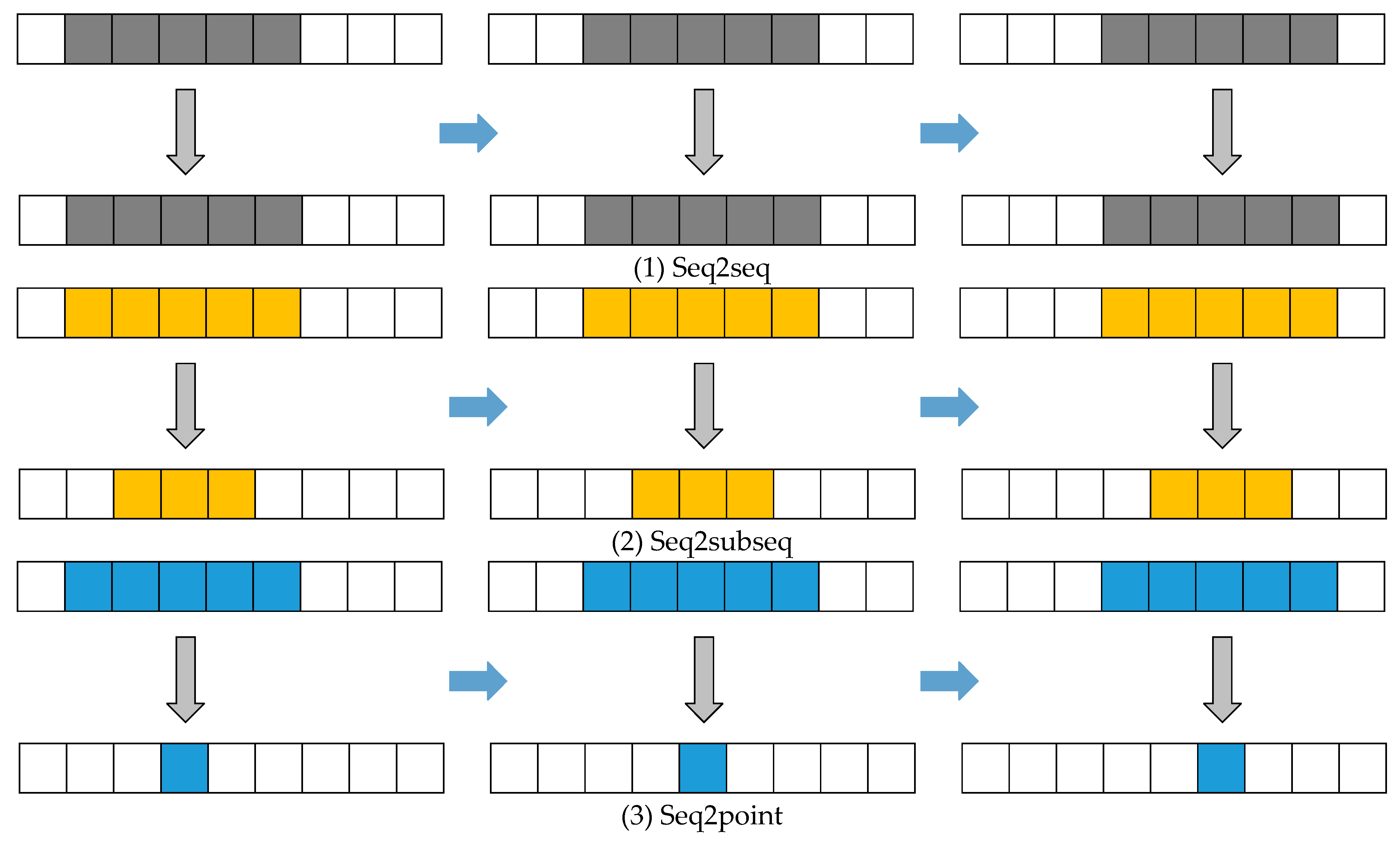
We conduct an experimental analysis on actual load data acquired from a large factory in China. The seq2seq, seq2point, and seq2subseq methods with sliding windows serve as benchmarks to compare the load decomposition ability of the new framework proposed in this paper. These three classic machine learning algorithms are used to demonstrate the superiority of our model. Finally, our model is compared with the representative MLSP model, highlighting its simplicity and efficiency.

The deep learning models are implemented by using Keras and TensorFlow. All the experiments in this paper involve training on a computer with a 12th-Gen Intel(R) Core(TM) i7-12700KF CPU at 3.60 GHz and an NVIDIA GeForce RTX 3070 Ti GPU.

4.1. Dataset Description

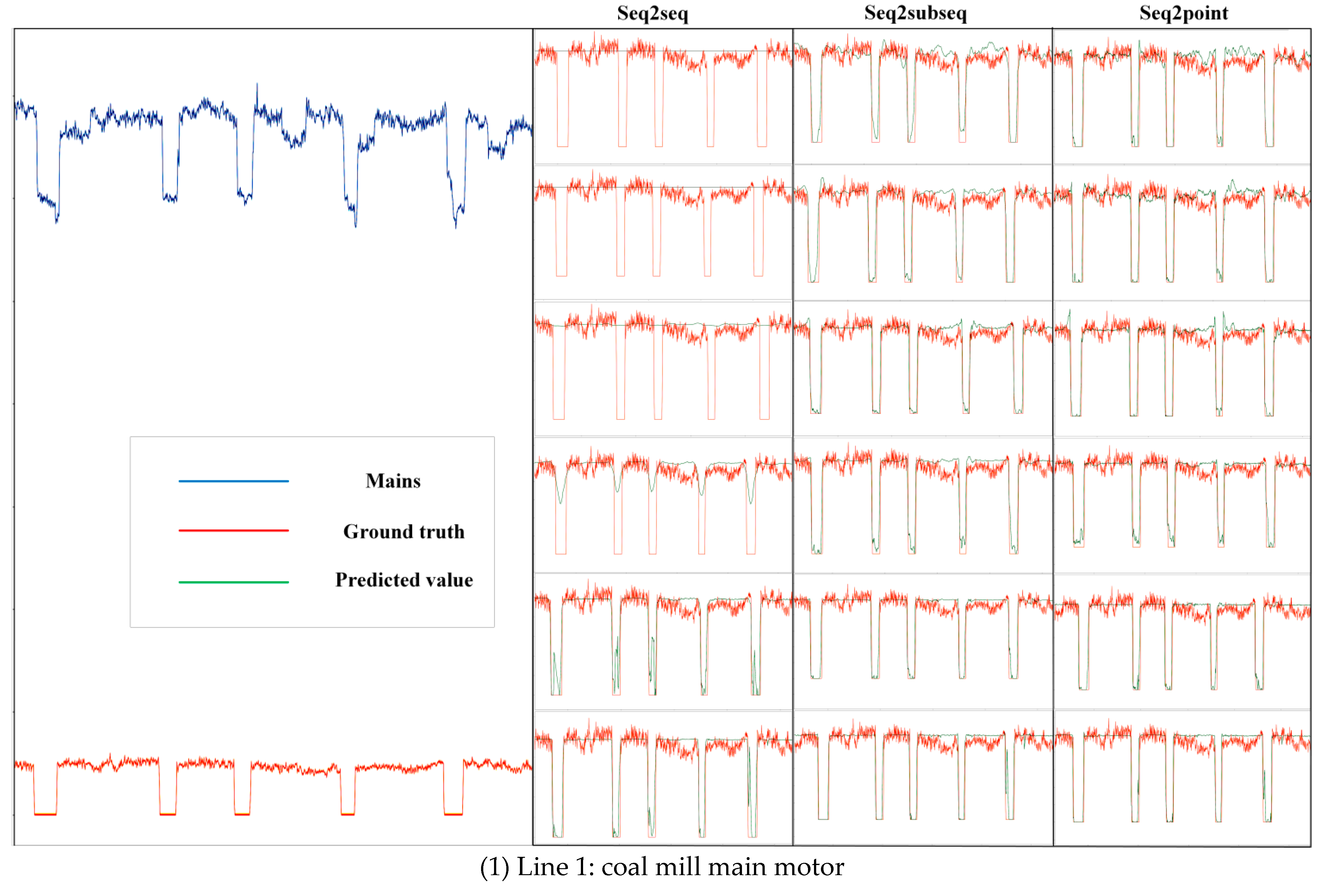
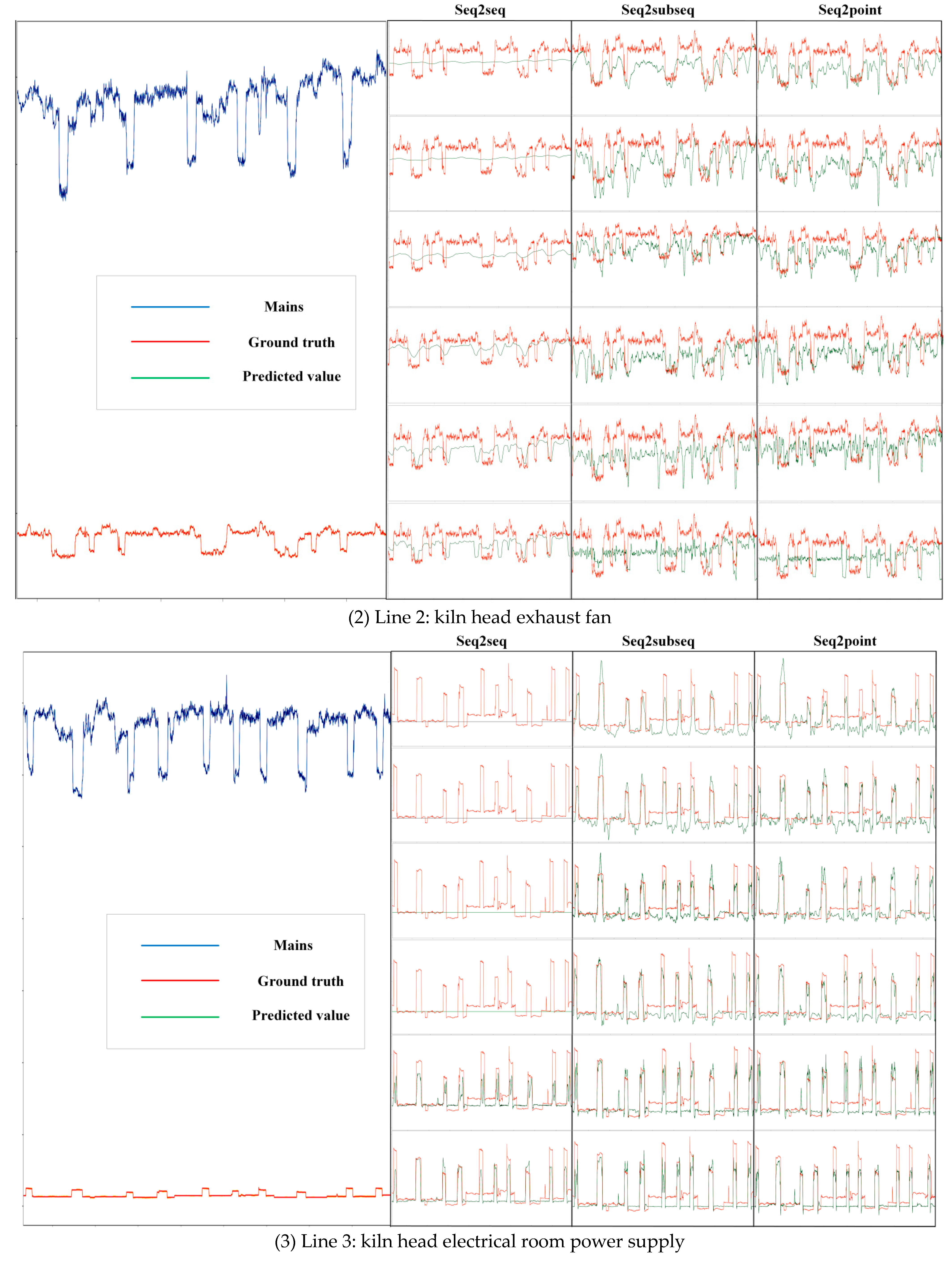
To verify the authenticity of the proposed method, an actual industrial load dataset is selected for experiments. The dataset contains data acquired from “1 February 2021 00:02:00” to “30 April 2021 23:58:00” at sampling frequencies of 1/120 Hz in the power room of a large factory in East China. Three different types of branch circuits are selected. Line 1, smooth closing equipment: coal mill main motor. Line 2, complex wave equipment: kiln head exhaust fan. Line 3, open wave equipment: kiln head electrical room power supply. The bus end collects voltage, current, power, admittance, and other related data. We collect the power data that need to be decomposed in each branch, such as the total active power.

4.2. Evaluation Indices

The mean absolute error (MAE) and mean squared error (MSE) are selected to evaluate the relationship between the predicted and actual values. In the field of load decomposition, these are common evaluation indicators that are used to evaluate the performance of forecasting models [31], where the MSE is the average of the squared differences between the predicted and true values. Compared with the MAE, the MSE can preserve the positive and negative information of errors and pay more attention to the impacts of large errors because after the error is squared, large errors receive higher weights [32]. The MAE is the average of the absolute values of the differences between the predicted values and the true values, which measures the average magnitude of the prediction error.

The formula for the MAE is:

$$MAE={\displaystyle \frac{{\displaystyle {\sum }_{i=1}^n\left|y_i-{\widehat{y}}_i\right|}}{n}}$$

(7)

The MSE formula is:

$$MSE={\displaystyle \frac{{\displaystyle {\sum }_{i=1}^n{\left(y_i-{\widehat{y}}_i\right)}^2}}{n}}$$

(8)

where $y_i$ represents the true value and ${\widehat{y}}_i$ represents the predicted value for a device at time $i$.

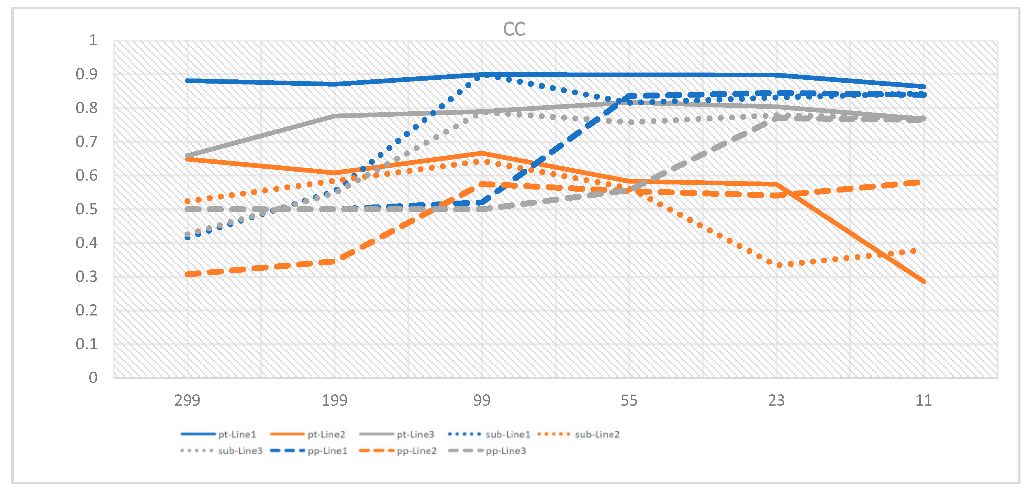
We focus on load disaggregation in complex industrial environments. For many industrial loads with complex fluctuations, it is not accurate to only use error indices to evaluate the distance relationship between the forecasts and actual values. The correlation coefficient (CC) can help us understand the relationship between the predictions and actual values, that is, the tightness of their linear relationship. The greater the correlation between them is, the more linear the correlation between the predicted trend and the actual values; therefore, we can disregard the interference caused by distance and consider the performance of the model from another perspective [28].

The CC is a statistic used to measure the strength of the relationship between two variables. It represents the degree of correlation between two random variables, with values ranging from −1 to 1, where −1 indicates a completely inverse correlation, 0 indicates an irrelevant correlation, and 1 indicates a completely positive correlation.

The calculation formula for the CC is as follows:

$$r={\displaystyle \frac{{\displaystyle {\sum }_{i=1}^n\left(x_i-\overline{x}\right)\left(y_i-\overline{y}\right)}}{\sqrt{{\displaystyle {\sum }_{i=1}^n{\left(x_i-\overline{x}\right)}^2}}\sqrt{{\displaystyle {\sum }_{i=1}^n{\left(y_i-\overline{y}\right)}^2}}}}$$

(9)

where x_i and y_i are the values of two variables at the ith sample point, and $\overline{x}$ and $\overline{y}$ are the mean values of these two variables, respectively.

By evaluating the performance of the model through three evaluation indicators, namely, the MAE, MSE, and CC, the decomposition performance of the model can be more thoroughly determined.

4.3. Experimental Settings

First, we analyze the window selection process under the sliding window method, taking three decomposition models, seq2point, seq2subseq, and seq2seq, as examples. Then, the influence of parameter selection in the proposed multi-electrical parameter-to-point method on the decomposition results is examined. We have conducted extensive comparative analyses. First, we compared the decomposition performance of our model with three sliding window models at their optimal window sizes. Second, we compared the decomposition capabilities of our model with three classic machine learning methods under the same parameter settings. Lastly, we compared our model with the MLSP model in terms of decomposition effectiveness and model efficiency. These comparisons better reflect the superiority of the model developed in this paper.

The relevant parameters to consider in the model of this paper include the batch size used when training the network (batch_size) and the number of dataset rows from which training data are selected (Crop). The batch_size is usually set to a power of 2, and it is set to 512 in the model proposed in this paper. Crop is set to 500,000 in the experiments presented in this paper. This is because the training portion of the employed industrial dataset has a single-parameter data length of 50,000. In this model, 10 electrical parameters are selected for joint training, so the data volume is 10 times the single-parameter data length, i.e., 500,000.

4.3.1. Analysis of the Window Size in the Sliding Window Approach

In the industrial environment, when the sampling frequency is 1/120 Hz, two sliding window methods are used, and different window sizes are set for experimental analysis purposes. Comparing the seq2point and seq2subseq methods (the seq2seq method has a poor effect, so it is not replicated in the paper), the window sizes are 299, 199, 99, 55, 23, and 11. The evaluation index changes produced in six cases are shown in a visual analysis of the decomposition results.

Figure 4 shows the MAE, MSE, and CC values obtained for the three types of loads. Figure 5 visualizes the decomposed image output under different window sizes.

Under the seq2point method, the MAE and MSE are optimized as the window size decreases, and the best results are obtained when the window sizes are 11, 99 and 11. In the seq2subseq method, the three distance metrics change more slowly, and the optimal results all occur at a window size of 99. According to the CC results, the gap between the results of the seq2subseq and seq2point methods is small. The CC of the seq2subseq method first increases and then decreases as the window size decreases, and the best result is obtained when the window size is at the midpoint.

These results are related to the natures of the two methods. In the seq2point method, the midpoint value is fitted by a window sequence, and the smaller the window is, the closer the result is to the actual value. In the seq2subseq method, a window sequence is used to fit a group of smaller windows. In this case, the smaller the window is, the better the result, but a balanced window length is needed.

However, if we analyze the actual decomposition images in Figure 5, the decomposition results of the two methods are poor. As the window size decreases for Line 1, although the load state changes are captured more accurately, the sudden error fluctuation also becomes larger, which is due to the disadvantages of the sliding window selection process. At this frequency scale, it is difficult to balance the amount of data and the time span. For Line 2, it is difficult to detect the differences from the decomposed images, which only roughly fit the true values, and the gaps in the evaluation indicators are small. Combining the images and data, better results are obtained when the window size is moderate. Line 3 is an open device with large interference; it is not a single device but rather the power supply of the whole branch room. In an industrial environment, a mix of industrial equipment and other circuits is often encountered, so it is very meaningful to study Line 3. For Line 3, we can see that the seq2point method obtains the most stable decomposition results when the window is the smallest, but it is of little practical significance because its error is too large, while the seq2subseq method obtains such results when the window size is 99.

In summary, when using the existing sliding window methods, it is difficult to obtain good decomposition results regardless of the window size. In practical applications, it is difficult to determine the actual operations of industrial loads, and it is difficult to monitor and analyze the equipment contained in a production line. To address this problem, we propose a new point-to-point NILM model that does not consider the window size.

4.3.2. Analysis of the Electrical Parameter Selection Process of the Multiple Electrical Parameter-to-Point Method

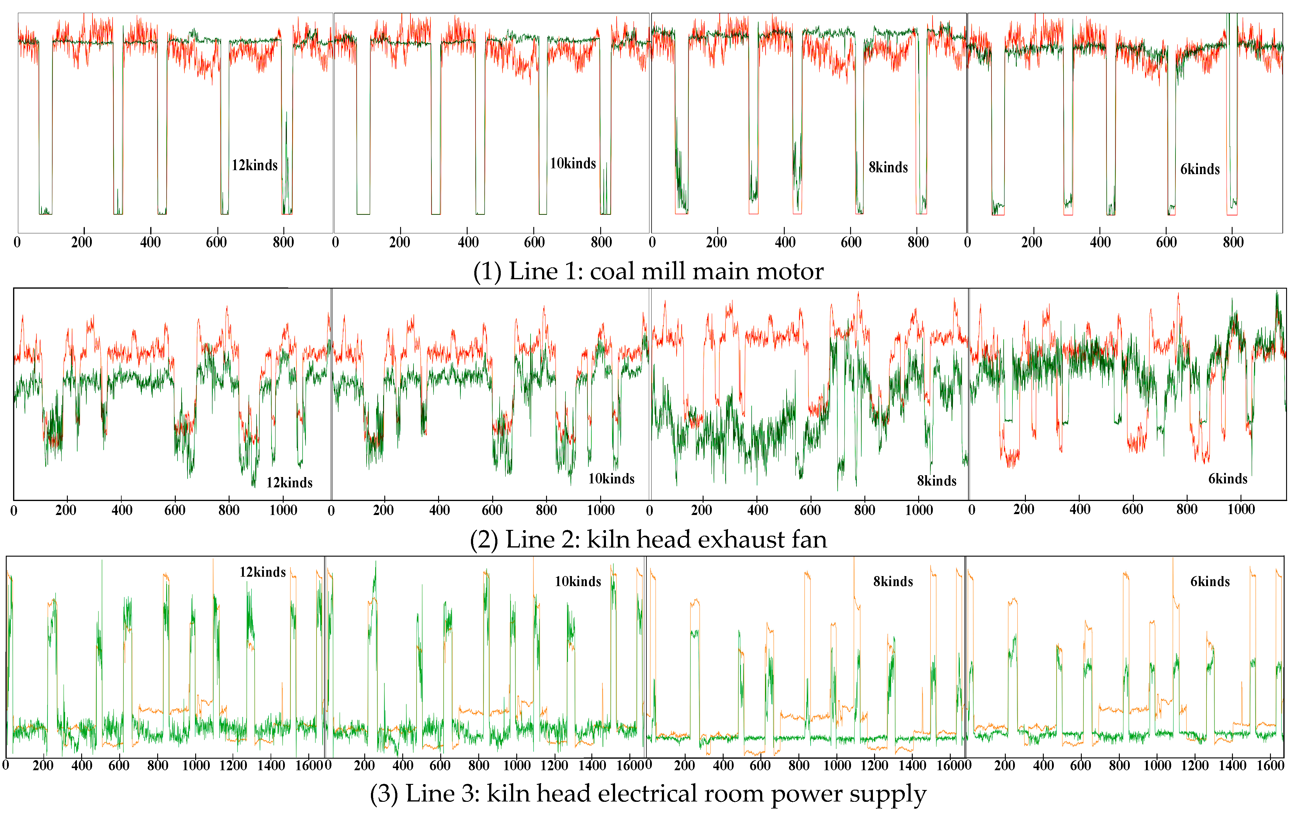
Taking the industrial dataset selected in this paper as an example, twelve kinds of electrical parameters are collected. Recently, several load decomposition studies have been conducted by adding reactive power and apparent power, and the results have shown that a certain improvement is provided by this approach. However, it is not certain that more features lead to a better effect. For example, the reactive power actually contains more power fluctuations, which negatively impact the decomposition results. Therefore, a correlation analysis of each electrical parameter at the bus end is carried out. The correlation analysis results obtained for each electrical parameter and the total active power can be seen in the table below because we chose to decompose the total active power of each branch. The reactive power has the worst correlation, and the current has the strongest correlation. Figure 6 shows the CC between each electrical parameter and the total active power. Four sets of parameters are set according to their correlations from low to high:

(1)

All 12 kinds of electrical parameters (A phase current; C phase current; A phase active power; C phase active power; total active power; A phase reactive power; total reactive power; A phase apparent power; C phase apparent power; total apparent power; A phase admittance; C phase admittance).

(2)

Ten kinds of electrical parameters after removing the A-phase reactive power and total reactive power.

(3)

Eight electrical parameters after removing the A-phase admittance and C-phase admittance.

(4)

Six electrical parameters after removing the A-phase active power and C-phase active power.

Table 2. The MAE, MSE, and CC values produced by the proposed model under different parameter combinations.

Line	Number of Electrical Parameters	MAE	MSE	CC
Line 1	12	0.0435	0.0054	0.8772
	10	0.0412	0.0049	0.9161
	8	0.0515	0.0078	0.8477
	6	0.0586	0.0098	0.7987
Line 2	12	0.0533	0.0037	0.7929
	10	0.0490	0.0034	0.7998
	8	0.1242	0.0184	0.2489
	6	0.1177	0.0263	0.1225
Line 3	12	0.03941	0.0031	0.7214
	10	0.0364	0.0025	0.7892
	8	0.0378	0.0038	0.6457
	6	0.0427	0.0037	0.7507

shows the performance of the model under different parameter combinations for three evaluation metrics.Through the MAE, MSE, and line chart analyses, the three types of loads yield the lowest distance indices when 10 kinds of electrical parameters are selected. At the same time, the CC line chart shows that the largest CC is still obtained when 10 kinds of parameters are selected. Combined with the example decomposition results presented in Figure 7, it can be seen that the decomposition effect of the model is optimized when the number of parameters is reduced from 12 to 10. However, when the number of parameters is reduced again, the decomposition effect deteriorates abruptly. All the indicators are optimal under 10 parameters, and the best decomposition results are also obtained at this time.

Combined with Figure 6, we can see that the reactive power has the lowest correlation, and it has a negative effect on the results obtained when the bus side contains reactive power. When the number of electrical parameters is further reduced, large errors appear in the decomposition results because the small number of parameters leads to a difficult fitting process. In Line 1, good degrees of fit are observed for both the descending and ascending mutations, but the shutdown state is more accurate only when 10 parameters are selected. This is highly important in an actual industrial environment, as its actual operations can be accurately analyzed. In Line 2, the decomposition results obtained for the two groups with 8 and 6 parameters are not meaningful, and the combination of data and images can effectively fit the true values under 10 parameters. In Line 3, when 10 parameters are used, the open state is more accurately understood, and the most accurate open load can be obtained. When 12 parameters are used, the fitting results are worse due to the interference of the reactive power, and the other two groups have large gaps, so it is difficult to accurately analyze the operations of the branch in practical applications.

4.3.3. Comparison between the Multi-Electrical Parameter-to-Point and Sliding Window Methods

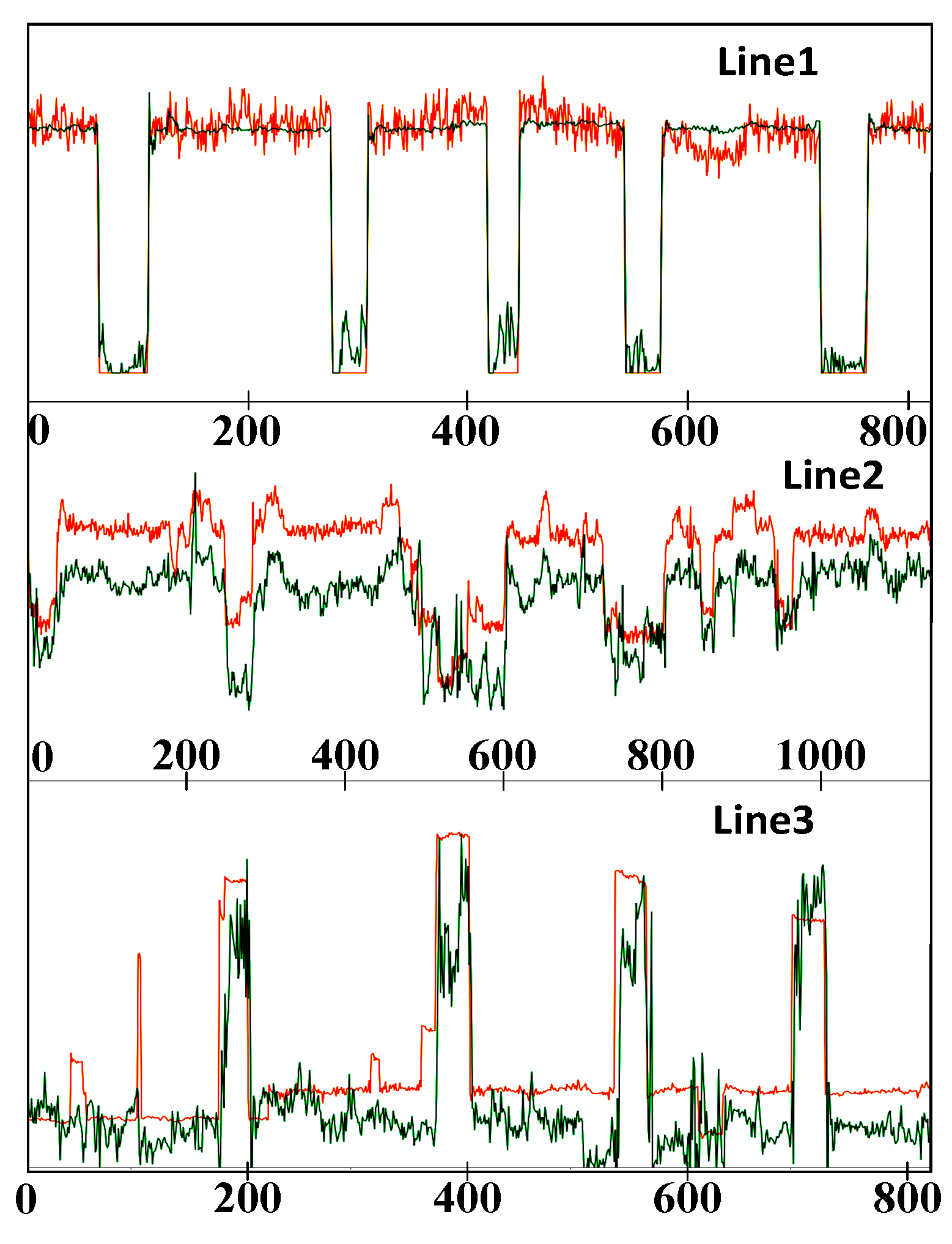
The results of the proposed multi-electrical parameter-to-point method are compared with those of the sliding window method under the optimal window. Figure 8 shows an example of the 3-branch decomposition results produced by the proposed multi-electric parameter-to-point (Mep2point) method, the seq2point method, and the seq2subseq method under the optimal window.

Table 3. MAEs, MSEs, and CCs produced by the Mep2point method and the seq2point seq2subseq methods under the optimal window.

Methods	Line	Windows	Mae	Mse	CC
Seq2seq	Line1	11	0.0510	0.0079	0.8388
	Line2	11	0.0554	0.0069	0.5816
	Line3	11	0.0388	0.0035	0.7645
Seq2subseq	Line1	99	0.0455	0.0058	0.8996
	Line2	99	0.0532	0.0036	0.6427
	Line3	99	0.0365	0.0025	0.7884
Seq2point	Line1	11	0.0494	0.0077	0.8634
	Line2	99	0.0656	0.0062	0.6661
	Line3	11	0.0394	0.0037	0.7674
Mep2point	Line1	\	0.0412	0.0049	0.9161
	Line2	\	0.049	0.0034	0.7998
	Line3	\	0.0364	0.0025	0.7892

shows MAEs, MSEs, and CCs produced by the Mep2point method and the seq2point seq2subseq methods under the optimal window.

Table 4. Degrees of improvement exhibited by the Mep2point method over the seq2point and seq2subseq methods under the optimal window.

Compare	Line	Windows	Mae	Mse	CC
Mep2point contrast Seq2seq	Line1	11	19.21%	37.97%	9.215%
	Line2	99	11.55%	50.72%	37.51%
	Line3	11	6.18%	28.57%	3.23%
Mep2point contrast Seq2subseq	Line1	99	9.45%	15.52%	1.83%
	Line2	99	7.89%	5.56%	24.44%
	Line3	99	0.27%	0.00%	0.10%
Mep2point contrast Seq2point	Line1	11	16.60%	36.36%	6.10%
	Line2	99	25.30%	45.16%	20.07%
	Line3	11	7.61%	32.43%	2.84%
Average increase rate			11.56%	28.03%	11.71%

shows the degrees of improvement exhibited by the Mep2point method over the seq2point and seq2subseq methods under the optimal window.

From the decomposition example, in Line 1, the proposed model exhibits good fitting results for the five downward trends; only the fifth downward trend has two very short increasing periods, but this does not interfere with the decomposition results. In contrast, the other two decomposition methods have large errors, and the seq2point method has more error fluctuations. However, the seq2subseq method is unable to accurately capture the zero-point information. This is because of the natures of these two methods. The seq2point method fits a point, so a greater disturbance is observed, while the seq2subseq method fits a segment of the given sequence, which can better fit the general curve but produces worse details.

In Line 2, the superiority of the proposed method can be clearly seen; it has a better fitting curve and better evaluation indices, while the other two methods are very weak in this case. In practice, the sliding window method cannot determine the actual operations of such industrial loads, while the proposed method can provide excellent decomposition results.

In the example presented for Line 3, ten rising trends are shown. Most of the ten rising trends yielded by the seq2point and seq2subseq methods do not reach the peak value, so the actual peak value is not decomposed. However, the method proposed in this paper more accurately decomposes the maximum value of the load. At this time, the fluctuations exhibited by the decomposition results are also more complex, leading to reductions in the evaluation indices because Line 3 is not industrial equipment but rather the total power supply of the room. Greater interference is observed, and the method developed in this paper selects a series of bus end parameters and a multiple of the interference, resulting in large fluctuations in its decomposition results, and the output curve can be gently fitted by performing noise reduction processing later. In practical applications, the seq2point and seq2subseq methods cannot obtain the actual operations of such industrial loads. Although the method proposed in this paper seems to fluctuate and be complex, its decomposition results are more practical for such loads, and they are closer to the actual operation values. In this application, the operation process is analyzed more accurately, which is helpful for monitoring and analyzing the line.

As mentioned in the review, under actual low-frequency industrial data, we select three representative workloads for a detailed comparative analysis. First, we compare the evaluation indicators and decomposition examples obtained under five window sizes ranging from 299 to 11 with the seq2point and seq2subseq methods as benchmarks. Due to the different properties of the two methods, the optimal results are obtained under different windows, but they still greatly deviate from the results shown in the example. Then, the influences of the electrical parameters on the decomposition results of the Mep2point method are analyzed, and the best result is obtained by choosing the optimal parameter combination after removing the reactive power. Finally, the Mep2point method is compared with the seq2point and seq2subseq methods under the optimal results in detail, and the superiority of the proposed model is verified by combining four evaluation indicators and decomposition example graphs.

Regarding the appropriate amount of input data for the presented model and the benchmark seq2point and seq2subseq methods, under the same numbers of network layers and output data, the input of the model proposed in this paper includes 10 electrical bus parameters, while the common sliding window method needs a longer time window; for example, the window size is set to 99 and 199. Hence, the amount of data represented also increases. Therefore, the data volume of the proposed model is lower and more efficient.

To resolve the contradiction between the window size and the time span that the sliding window method cannot balance in a low-frequency environment, we propose a multi-electrical parameter-to-point load decomposition method and verify the superiority of the model on actual industrial data. Compared with the sliding window method, the model in this paper can better obtain the actual operation trends of the industrial load. In actual applications, load operations can be monitored more accurately, which is helpful for the monitoring and analysis of the equipment in a production line.

4.3.4. Comparison between the Mep2point Method and Machine Learning Methods

In this paper, the proposed model selects different types of electrical parameters at the bus end as inputs, while the number of electrical parameters is usually only 10, and the amount of data is small.

In cases with less data, machine learning may be more suitable than deep learning. Machine learning can use traditional algorithms for prediction and classification. These algorithms have relatively small data demands, and they can also produce good results for small-scale datasets.

To verify the superiority of the proposed model, three machine learning algorithms, namely, support vector regression (SVR), linear regression, and KNN, are selected to analyze and process the data.

The following table shows the MAEs, MSEs, and CCs yielded by the three machine learning algorithms under the two parameter settings.

Table 5. MAEs, MSEs, and CCs produced by the three machine learning methods under different parameter combinations.

Line	Number of Electrical Parameters	Methods	Mae	Mse	CC
Line1	12	Linear regression	0.0679	0.0128	0.8495
		Svr	0.0521	0.00586	0.8717
		Knn	0.0474	0.00616	0.8656
		Mep2point	0.0435	0.0054	0.8772
	10	Linear regression	0.0677	0.0127	0.8535
		Svm	0.0521	0.00596	0.8737
		Knn	0.0478	0.00609	0.8658
		Mep2point	0.0412	0.0049	0.9161
Line2	12	Linear regression	0.0533	0.00387	0.7611
		Svr	0.0501	0.00328	0.7847
		Knn	0.0557	0.00419	0.7179
		Mep2point	0.0533	0.0037	0.7929
	10	Linear regression	0.0535	0.00392	0.7505
		Svr	0.0506	0.00332	0.7893
		Knn	0.0549	0.00408	0.7177
		Mep2point	0.0490	0.0034	0.7998
Line3	12	Linear regression	0.0442	0.00411	0.6748
		Svr	0.0353	0.00276	0.7459
		Knn	0.0392	0.00325	0.7108
		Mep2point	0.03941	0.0031	0.7214
	10	Linear regression	0.0443	0.00413	0.6724
		Svr	0.0356	0.00285	0.7369
		Knn	0.0388	0.00321	0.7145
		Mep2point	0.0364	0.0025	0.7892

compares the MAEs, MSEs, and CCs yielded by the four models under the two parameter combinations. Among the three machine learning methods, SVR produces optimal results in most cases, but a large gap remains between SVR and the Mep2point method proposed in this paper. However, the machine learning model has a good advantage in that its training time can be ignored, so it has good application prospects when utilizing the multiple electrical parameters employed in this paper in some characteristic scenarios.

4.3.5. Comparison between the Mep2point Method and MLSP Methods

The core idea of the model in this paper is to avoid the use of sliding window methods, which are difficult to bypass in the field of non-intrusive load decomposition. Compared to sliding window models, our model, on the one hand, avoids the challenging issue of window length selection and, on the other hand, significantly reduces the model complexity.

The MLSP model proposed a new framework that combines multi-channel electrical parameters with the sliding window model to expand the amount of data represented within the same window length, addressing the issue of feature loss caused by a small sliding window. However, on one hand, the increase in data volume leads to an increase in computational load and training time, resulting in higher model complexity. On the other hand, in the industrial environment, where there is more interference, the MLSP method also causes this interference to multiply during training, leading to a significant amount of error fluctuation in the decomposition results.

Demonstrate the superiority of the model in this paper by comparing it with an MLSP method that selects a variety of bus-end electrical parameters, as proposed in the paper [29].

Table 6. MAEs, MSEs, and CCs produced by the two models.

Methods	Line	Number of Electrical Parameters	Windows	Mae	Mse	CC
Mep2point	Line1	10	\	0.0412	0.0049	0.9161
	Line2		\	0.049	0.0034	0.7998
	Line3		\	0.0364	0.0025	0.7892
MLSP	Line1		11	0.0456	0.0059	0.8734
	Line2		11	0.0592	0.0046	0.7577
	Line3		11	0.0421	0.0036	0.6935

presents the three evaluation metrics for the two models.

Table 7. Training time for both models.

Methods	Windows	Number of Electrical Parameters	Batch Size	Epochs	Time
Mep2point	\	10	512	100	1201.1 s
MLSP	11				14,113.4 s

provides the model training time when the number of electrical parameters, batch size, and epochs are the same. Figure 9 illustrates the decomposition examples of three lines under the MLSP model.

Combining the data from the two tables, it can be seen that the evaluation metrics of the model in this paper are slightly better than those of the MLSP model. At the same time, the training time of the model in this paper is only one-tenth of that of the MLSP model.

Comparing the decomposition Examples of the three lines of the two models in Figure 8 and Figure 9. In Line 1, the capture results of the model in this paper are more accurate, while the MLSP model exhibits a large number of erroneous fluctuations at the bottom. In Line 2, the MLSP model performs better in the actual decomposition of complex disturbances, outperforming the model in this paper. Comparing Line 3, there is no significant difference in the decomposition capabilities between the two models. By analyzing the principles of the two models, it can be known that the model in this paper requires less training data compared to the MLSP model, which reduces the interference of a large amount of data, lowers the model’s complexity, and therefore significantly improves the model’s operational efficiency. At the same time, it has better decomposition capabilities for loads with clear operating states, but its decomposition capabilities for complex operating loads are weaker.

In summary, an experimental analysis is conducted on actual industrial datasets using seq2seq, seq2point, and seq2subseq as benchmark methods. The experimental results show that compared to the baseline methods, the approach proposed in this paper is superior in terms of its parameter indicators and actual image decomposition results. However, at the same time, compared with the benchmark methods, the

The universality of the proposed method is also reduced, as it requires more types of electrical parameter data at the bus end. In addition, because of the characteristics of the input data, three machine learning methods are added to the comparison. From the indicator perspective, the model proposed in this paper has great advantages, but by using multiple parameters as the model inputs, the machine learning methods still have application prospects. Finally, a comparison was made between the model in this paper and the MLSP model, on one hand, it reflects the different advantages in different application scenarios, and on the other hand, it demonstrates the simplicity and efficiency of the model in this paper.

5. Conclusions

We propose an NILM model for industrial load decomposition that converts multiple electrical parameters to points. To resolve the difficulty of selecting the optimal window size under the sliding window method, a variety of electrical parameter data are used to fit the target load to be decomposed. This paper presents a non-intrusive decomposition method that does not use a sliding window, thereby overcoming the difficulty of choosing a sliding window size. This provides readers with a new solution.

The main contributions of this paper are as follows.

• Because the sliding window method has difficulty selecting the optimal window and its decomposition effect is poor, a new point-to-point load decomposition method is proposed.
• The relationships between the performances of three advanced models under the sliding window method with different window sizes are analyzed on a real industrial environment dataset.
• On the actual industrial environment dataset, the influences of different electrical parameter correlations on the performance of the proposed model are analyzed.
• By taking three classic machine learning algorithms as benchmarks and comparing their model decomposition capabilities in different cases, this paper shows the superiority of the proposed model and reflects the scalability of selecting electrical parameters as the model inputs.
• Comparing with the MLSP model that utilizes a variety of bus-end data and combines sequence-to-point, the model in this paper demonstrates its simplicity in data usage, efficient training, and excellent performance.

However, our model still has some potential limitations. The common decomposition method selects only one electrical parameter at the bus end, but we choose dozens of parameters. At this time, the interference caused by the data increases exponentially, so the decomposition results exhibit large fluctuations when a load with a large amount of noise is decomposed. At the same time, the model developed in this paper must obtain a variety of electrical parameter data at the bus end, which is difficult to execute. At present, most data only include a few types of electrical parameters at the bus end.

In future research, on the one hand, noise reduction must be carried out on the input data to obtain more stable decomposition results, and on the other hand, much room remains for improving the identification effects produced for loads with complex fluctuations. It is also necessary to extend the data from a single electrical parameter to improve the applicability of the proposed method. In the future, complex industrial load types must be further studied to improve the fitting accuracy of the developed model so that it can be better applied in real environments, and the generalizability of the model must be improved.