Comparative and Sensibility Analysis of Cooling Systems

Abstract

As the global average temperature has increased due to climate change, the use of air conditioning equipment for cooling homes has become more popular. Inverter equipment is advertised as a better energy option than systems with an on/off control; however, there is a lack of sufficient studies to prove this. This work aims to analyze and compare the electricity consumption associated with cooling equipment with an on/off control and inverter equipment. A heat transfer model coupled with energy balance for a room is developed and implemented in Python 3.12. The indoor temperature is controlled by simulating an on/off control and a PID control for the inverter system. Subsequently, the electricity consumption of the two systems is compared, and a sensitivity analysis is performed to determine which variables have the greatest impact on electricity consumption. The results show that the inverter equipment has lower electricity consumption compared to the equipment with the on/off control. However, the sensitivity analysis shows that the indoor temperature set point plays a more relevant role since a 15% variation in its value impacts electricity consumption by up to 77%.

1. Introduction

Worldwide, the construction sector consumes between 30% and 40% of the final energy and is responsible for 19% of greenhouse gas emissions [1,2,3]. In addition, it is expected to increase its energy consumption at a minimum annual rate of 1.5% [4]. The operation of heating, ventilation, and air conditioning (HVAC) equipment accounts for about 50% of the energy used in the building sector [5].

The indoor environment of buildings has a direct impact on health and comfort; HVAC equipment improves thermal quality and indoor air quality and is the most common equipment for maintaining thermal comfort. Additionally, people spend about 90% of their time indoors [6,7]. However, the operation of HVAC equipment represents higher electricity consumption [5].

It is estimated that 20% of the electricity consumed in buildings is used for space cooling by means of air conditioning equipment and ventilators [8]. Moreover, these numbers are expected to increase due to global economic growth, the large displacement of people from villages to cities, and the extension of built-up areas [9,10]. Thus, as incomes and quality of life increase, more people will buy and use air conditioning equipment and fans, especially those located in the warmer parts of the world. If no action is taken, energy consumption for space cooling will triple by 2050 compared to consumption in 2018 [8].

To meet the challenge of addressing the growing energy demand, recent research is focused on optimizing demand management for cost reduction by shifting peak demand [11]. Efforts are also being made to optimize the performance of HVAC equipment, as it is crucial for energy savings, energy efficiency, and sustainability. Optimizing energy consumption through HVAC equipment control strategies has been explored.

In buildings, HVAC equipment control strategies are aimed at controlling their operation to ensure adequate thermal comfort conditions for the occupants. Hassanpour et al. [1] mention that up to 30% energy savings can be achieved with a combination of improved control strategies and the elimination of faults in the operation of HVAC equipment.

The most recent studies are focused on fault diagnosis and monitoring [12,13,14,15] and in the implementation of advanced control strategies based on artificial intelligence [16]. However, in developing countries, the acquisition of air conditioning (AC) equipment is limited by income and, in some cases, cannot be purchased; in fact, it is estimated that in Mexico, between 4.9 and 7.2 million households need but lack air conditioning equipment [17]. Therefore, in these countries, many of the AC units are old, with conventional feedback control strategies (on/off), and technologies with proportional–integral–derivative (PID) control strategies are being acquired gradually by users, especially by users of the residential sector for which their acquisition and operation can represent a significant expense [18,19].

The on/off control strategy can sometimes cause AC equipment to operate at full load when only a fraction of the load is needed, whereas PID control provides precise control [20].

Although, in 2014, it was estimated that in Mexico, 3% of the total electricity demand is due to the air conditioning equipment for the residential sector [21], at present, this percentage is unknown as there are no recent studies regarding this matter; however, this number is expected to increase, especially with the recent heat waves the country is experiencing. Most of this AC equipment operate with the on/off control strategy, and similar equipment will likely continue to be acquired as they represent a lower investment compared to AC equipment with PID control strategies.

This work aims to compare the electricity consumption associated with AC equipment for cooling considering two control strategies: on/off and inverter. The latter strategy involves the implementation of a PID control to achieve the desired temperature. To perform the analysis, the heat transfer through the roof of the enclosure is modeled; this model is coupled to an energy balance to determine the interior temperature of the enclosure and control the operating power of the AC equipment; the operation of the equipment is also modeled, and the complete model is implemented in Python. Subsequently, the electricity consumption of the two systems is compared. Finally, a sensitivity analysis is performed to determine the impact on electricity consumption of the following variables: thickness, density, and thermal conductivity of the building material, as well as external wind speed, incident solar radiation, ambient temperature, air flow entering the enclosure, enclosure height, and desired temperature.

This work consists of a description of the methodology used for the evaluation of the performance of the AC equipment, in which the heat transfer processes and the equations that model it are described, as well as the implemented control strategies. Also, the numerical solution of the model and the implementation of the inverter control strategy (PID) are presented. Subsequently, the results found through the computational simulations performed in Python are shown. The subsequent section presents a discussion of these results and their analysis. Finally, the conclusions section is presented.

2. Methodology

The methodology can be summarized in the following points:

• Development of the dynamic heat transfer model
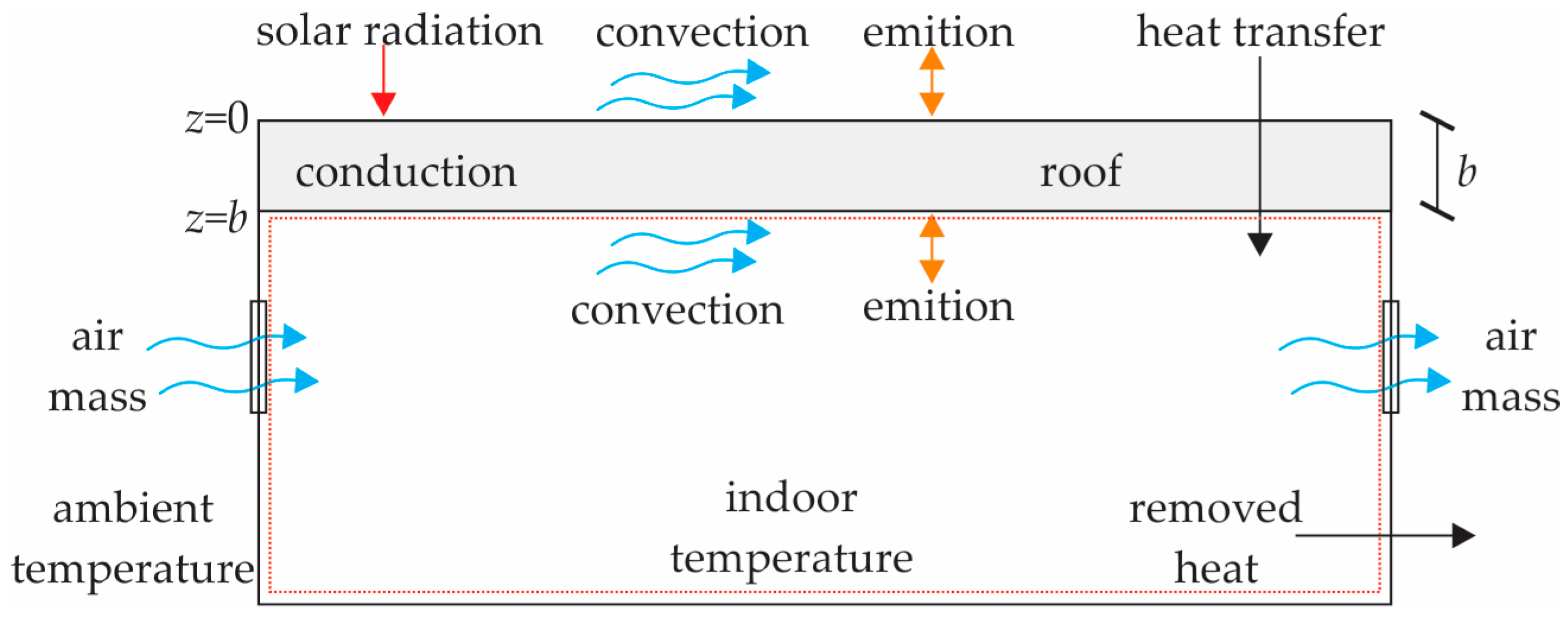
  • In this step, we first describe the dynamic model of one-dimensional heat transfer via conduction through the roof of the building. The boundary conditions are given, and the equations necessary to calculate the heat fluxes are presented.
  • Subsequently, the energy balance for the interior of the building, considering an open system, is presented, and the equations that couple this balance with the heat transfer model are shown.
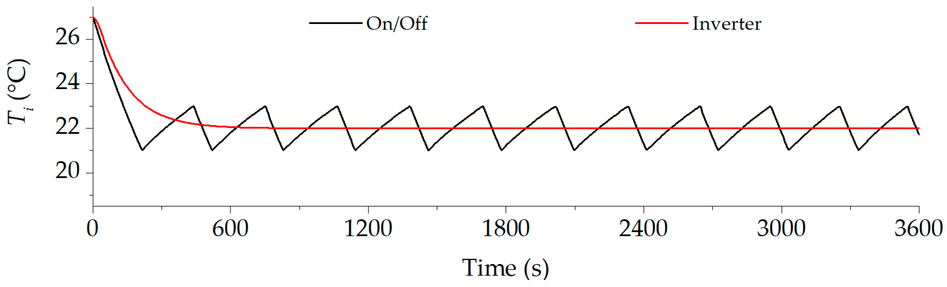
  • The energy balance shows how the temperature inside the building changes, which is desired to control by means of AC equipment. Therefore, two control strategies are presented that are coupled to the energy balance to remove heat from the building if necessary. The first strategy is the on/off control; the second strategy is a PID control to simulate the behavior of inverter equipment.
• Numerical solution method
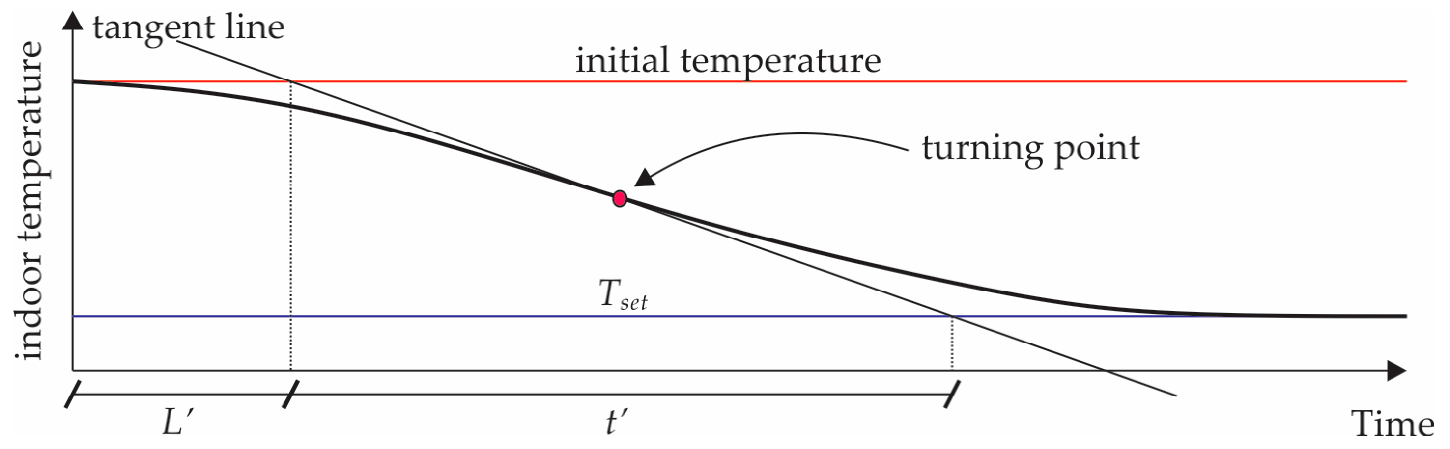
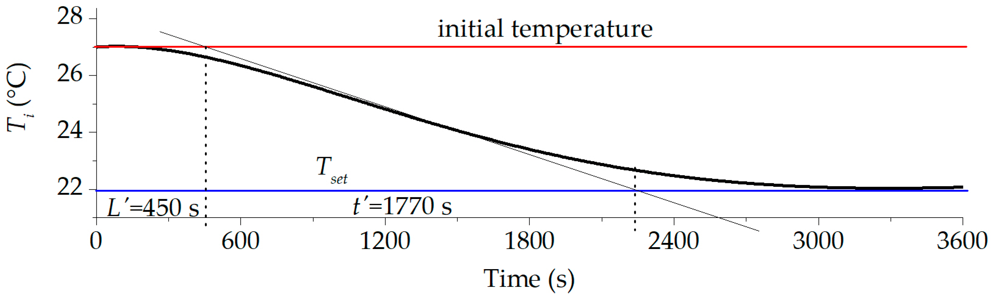
  • In this step, the discrete form of the differential equations previously presented is shown. The Euler method is implemented in Python to obtain the interior temperature of the building for different times. The control strategies are coupled, and the PID strategy is tuned; that is, the values of the proportional, integral, and derivative constants are determined. The use of Python is highly advantageous due to its open-source nature and the extensive range of libraries that facilitate modeling in engineering. In this study, thermal properties of air and refrigerants libraries were used. Unlike licensed software, which often incurs high costs, these types of models can be implemented and executed on any device, regardless of its operating system or computing capacity. This feature is particularly beneficial for on-site testing and trials with short periods of time.
• Application to the base case
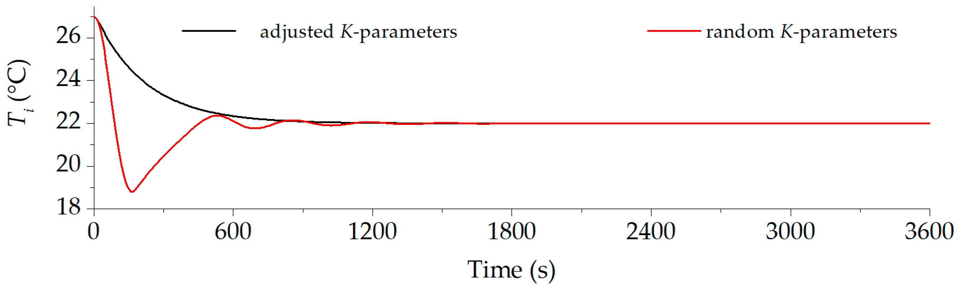
  • The variables of the base case are taken to verify that the control strategies work properly; this can be seen by analyzing the evolution over time of the temperature inside the building.
  • Once the correct operation of the control strategies has been verified, the electricity consumption of the two control strategies for the base case is compared.
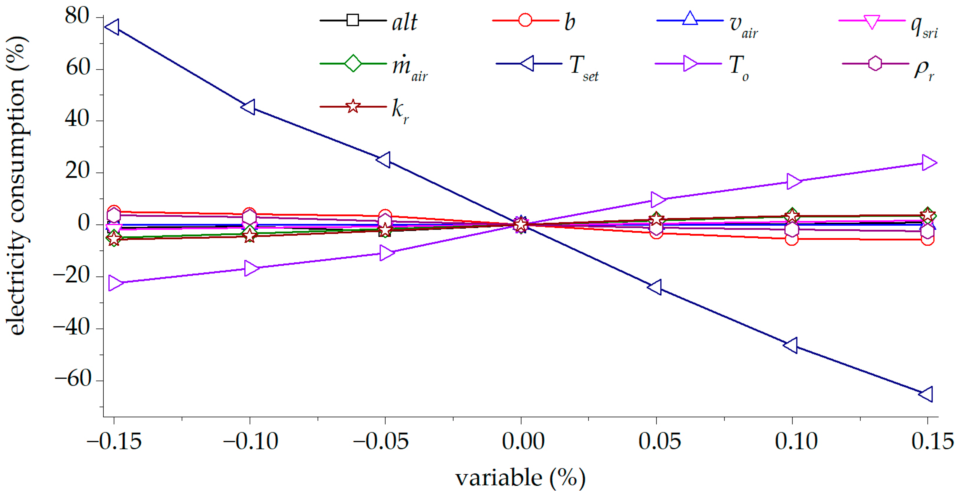
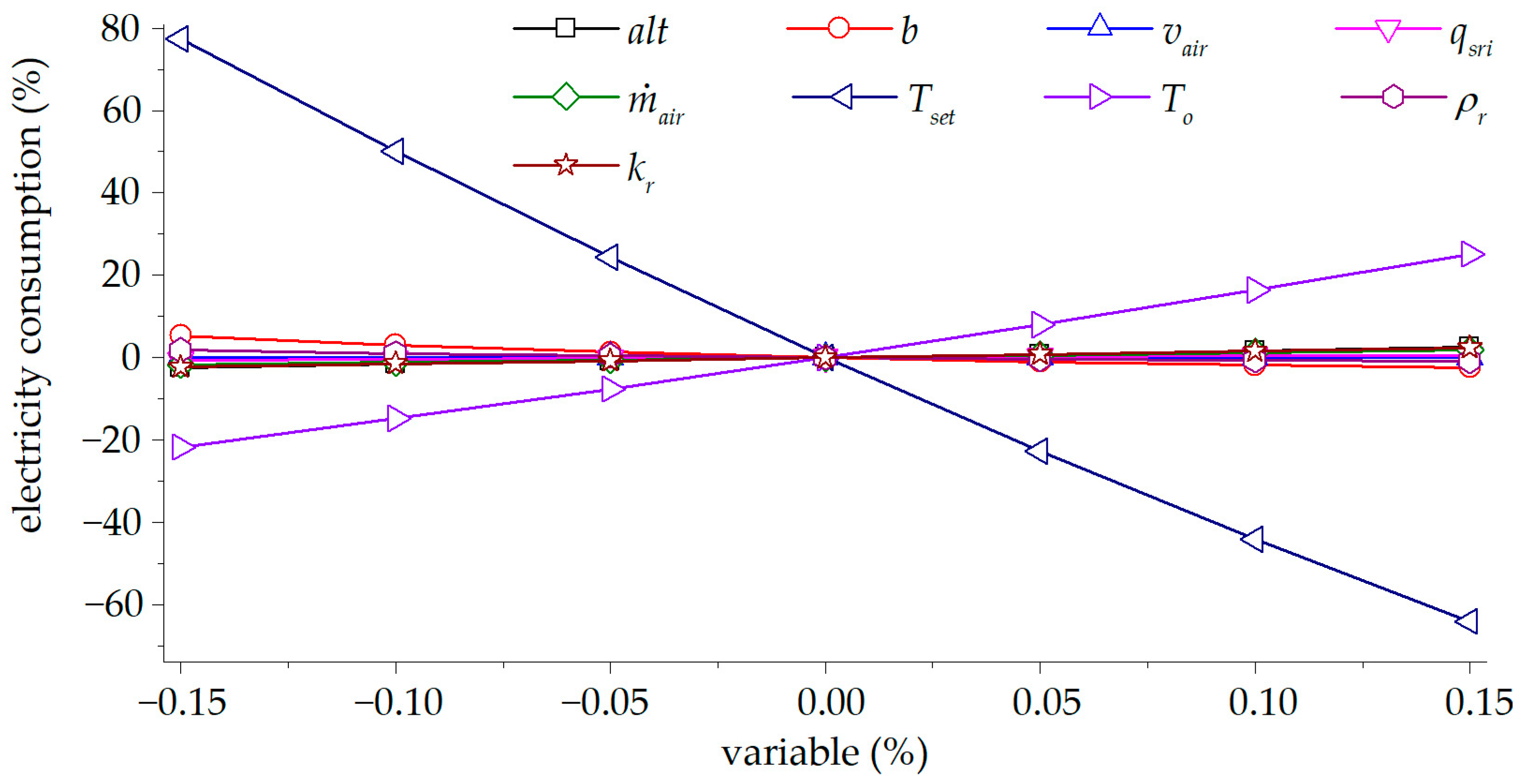
  • Finally, a sensitivity analysis is performed to determine the variables that have the greatest impact on electricity consumption.

The proposed methodology is developed below.

2.1. Dynamic Heat Transfer Model

In this section, the one-dimensional dynamic heat transfer model for the building is developed. The dynamic heat transferred via conduction in one dimension through the roof is given by

$${\rho }_{r}C{p}_r{\displaystyle \frac{\partial T}{\partial t}}=k_r{\displaystyle \frac{{\partial }^{2}T}{\partial z^2}}\hspace{0.17em}\hspace{0.17em}\hspace{0.17em}\hspace{0.17em}\hspace{0.17em}\hspace{0.17em}\hspace{0.17em}\hspace{0.17em}\hspace{0.17em}\hspace{0.17em}\hspace{0.17em}\hspace{0.17em}\hspace{0.17em}\hspace{0.17em}\hspace{0.17em}\left[{\displaystyle \frac{\mathrm{W}}{{\mathrm{m}}^3}}\right],$$

(1)

where $\rho$ is the density, Cp is the specific heat, T is the temperature, k is the thermal conductivity, z is the direction of heat transfer, t is the time, and the subscript r refers to the roof material. Equation (1) has the following boundary conditions:

$${\mathrm{B}.\mathrm{C}.1 -k_r{\displaystyle \frac{dT}{dz}}|}_{z=0}={\dot{q}}_{sr}+{\dot{q}}_{cv,o}+{\dot{q}}_{em,o}\hspace{0.17em}\hspace{0.17em}\hspace{0.17em}\hspace{0.17em}\hspace{0.17em}\hspace{0.17em}\hspace{0.17em}\hspace{0.17em}\hspace{0.17em}\hspace{0.17em}\hspace{0.17em}\hspace{0.17em}\hspace{0.17em}\hspace{0.17em}\hspace{0.17em}\left[{\displaystyle \frac{\mathrm{W}}{{\mathrm{m}}^2}}\right],$$

(2)

$$\mathrm{B}.\mathrm{C}.2 {-k_r{\displaystyle \frac{dT}{dz}}|}_{z=b}={\dot{q}}_{cv,i}+{\dot{q}}_{em,i}\hspace{0.17em}\hspace{0.17em}\hspace{0.17em}\hspace{0.17em}\hspace{0.17em}\hspace{0.17em}\hspace{0.17em}\hspace{0.17em}\hspace{0.17em}\hspace{0.17em}\hspace{0.17em}\hspace{0.17em}\hspace{0.17em}\hspace{0.17em}\hspace{0.17em}\left[{\displaystyle \frac{\mathrm{W}}{{\mathrm{m}}^2}}\right],$$

(3)

where ${\dot{q}}_{sr}$ is the heat gained by solar radiation, ${\dot{q}}_{cv}$ is the heat transferred by convection, and ${\dot{q}}_{em}$ is the net heat flux by emission. The parameter b is the roof thickness, so z = 0 is the outer surface of the roof and z = b is the inner surface (see Figure 1). The subscripts o and i indicate the outside and inside of the building, respectively. These heat fluxes are calculated from

$${\dot{q}}_{sr}=\alpha {\dot{q}}_{sri}\hspace{0.17em}\hspace{0.17em}\hspace{0.17em}\hspace{0.17em}\hspace{0.17em}\hspace{0.17em}\hspace{0.17em}\hspace{0.17em}\hspace{0.17em}\hspace{0.17em}\hspace{0.17em}\hspace{0.17em}\hspace{0.17em}\hspace{0.17em}\hspace{0.17em}\left[{\displaystyle \frac{\mathrm{W}}{{\mathrm{m}}^2}}\right],$$

(4)

$${\dot{q}}_{cv,o}=h_o\left(T_o-{T|}_{z=b}\right)\hspace{0.17em}\hspace{0.17em}\hspace{0.17em}\hspace{0.17em}\hspace{0.17em}\hspace{0.17em}\hspace{0.17em}\hspace{0.17em}\hspace{0.17em}\hspace{0.17em}\hspace{0.17em}\hspace{0.17em}\hspace{0.17em}\hspace{0.17em}\hspace{0.17em}\left[{\displaystyle \frac{\mathrm{W}}{{\mathrm{m}}^2}}\right],$$

(5)

$${\dot{q}}_{em,o}=\epsilon \sigma \left(T_{sky}-{T^4|}_{z=b}\right)\hspace{0.17em}\hspace{0.17em}\hspace{0.17em}\hspace{0.17em}\hspace{0.17em}\hspace{0.17em}\hspace{0.17em}\hspace{0.17em}\hspace{0.17em}\hspace{0.17em}\hspace{0.17em}\hspace{0.17em}\hspace{0.17em}\hspace{0.17em}\hspace{0.17em}\left[{\displaystyle \frac{\mathrm{W}}{{\mathrm{m}}^2}}\right],$$

(6)

$${\dot{q}}_{cv,i}=h_i\left({T|}_{z=0}-T_i\right)\hspace{0.17em}\hspace{0.17em}\hspace{0.17em}\hspace{0.17em}\hspace{0.17em}\hspace{0.17em}\hspace{0.17em}\hspace{0.17em}\hspace{0.17em}\hspace{0.17em}\hspace{0.17em}\hspace{0.17em}\hspace{0.17em}\hspace{0.17em}\hspace{0.17em}\left[{\displaystyle \frac{\mathrm{W}}{{\mathrm{m}}^2}}\right],$$

(7)

$${\dot{q}}_{em,i}=\epsilon \sigma \left({T^4|}_{z=0}-T_{alr}^4\right)\hspace{0.17em}\hspace{0.17em}\hspace{0.17em}\hspace{0.17em}\hspace{0.17em}\hspace{0.17em}\hspace{0.17em}\hspace{0.17em}\hspace{0.17em}\hspace{0.17em}\hspace{0.17em}\hspace{0.17em}\hspace{0.17em}\hspace{0.17em}\hspace{0.17em}\left[{\displaystyle \frac{\mathrm{W}}{{\mathrm{m}}^2}}\right],$$

(8)

where $\alpha$ is the absorptivity of the building element, ${\dot{q}}_{sri}$ is the incident solar irradiance, $h$ is the convective heat transfer coefficient, $\epsilon$ is the thermal emissivity, $\sigma$ is the Stefan–Boltzmann constant, $T_i$ is the air temperature inside the building, $T_o$ is the ambient temperature, $T_{sky}$ is the sky temperature, and $T_{alr}$ is the temperature of the surroundings, i.e., the temperature of the walls and floor inside the building. There are many methods by which to determine $T_{sky}$; however, a practical way is to consider that $T_{sky}=T_o-13\mathrm{K}$ [22].

Convective heat transfer coefficients are calculated from

$$\mathrm{Nu}={\displaystyle \frac{h{L}_c}{k_{air}}}\hspace{0.17em}\hspace{0.17em}\hspace{0.17em}\hspace{0.17em}\hspace{0.17em}\hspace{0.17em}\hspace{0.17em}\hspace{0.17em}\hspace{0.17em}\hspace{0.17em}\hspace{0.17em}\hspace{0.17em}\hspace{0.17em}\hspace{0.17em}\hspace{0.17em}\left[\mathrm{dimensionless}\right],$$

(9)

where $L_c$ is the characteristic length of the heat transfer surface, Nu is the dimensionless Nusselt number, and the subscript air refers to the properties of the air, either evaluated at the outer film temperature, $T_{f,o}$, or at the inner film temperature, $T_{f,i}$, which are given by

$$T_{f,o}={\displaystyle \frac{T_o+{T|}_{z=0}}{2}}\hspace{0.17em}\hspace{0.17em}\hspace{0.17em}\hspace{0.17em}\hspace{0.17em}\hspace{0.17em}\hspace{0.17em}\hspace{0.17em}\hspace{0.17em}\hspace{0.17em}\hspace{0.17em}\hspace{0.17em}\hspace{0.17em}\hspace{0.17em}\hspace{0.17em}\left[°\mathrm{C}\right],$$

(10)

$$T_{f,i}={\displaystyle \frac{T_i+{T|}_{z=b}}{2}}\hspace{0.17em}\hspace{0.17em}\hspace{0.17em}\hspace{0.17em}\hspace{0.17em}\hspace{0.17em}\hspace{0.17em}\hspace{0.17em}\hspace{0.17em}\hspace{0.17em}\hspace{0.17em}\hspace{0.17em}\hspace{0.17em}\hspace{0.17em}\hspace{0.17em}\left[°\mathrm{C}\right].$$

(11)

The calculation of the Nusselt number (Nu) depends on the type of convection, which can be free or forced. The following sections describe the calculation of the Nusselt number for the roof under conditions of forced convection and free convection.

Forced convection [23]:

$$\mathrm{Nu}={\displaystyle \frac{0.3387{\mathrm{Pr}}^{\raisebox{1ex}{$1$}\!\left/ \!\raisebox{-1ex}{$3$}\right.}{\mathrm{Re}}^{\raisebox{1ex}{$1$}\!\left/ \!\raisebox{-1ex}{$2$}\right.}}{{\left[1+\left(\raisebox{1ex}{$0.0468$}\!\left/ \!\raisebox{-1ex}{${\mathrm{Pr}}^{\raisebox{1ex}{$2$}\!\left/ \!\raisebox{-1ex}{$3$}\right.}$}\right.\right)\right]}^{\raisebox{1ex}{$1$}\!\left/ \!\raisebox{-1ex}{$4$}\right.}}}\hspace{0.17em}\hspace{0.17em}\hspace{0.17em}\hspace{0.17em}\hspace{0.17em}\hspace{0.17em}\hspace{0.17em}\hspace{0.17em}\hspace{0.17em}\hspace{0.17em}\hspace{0.17em}\hspace{0.17em}\hspace{0.17em}\hspace{0.17em}\hspace{0.17em}\left[\mathrm{dimensionless}\right],$$

(12)

where Pr is the Prandtl number and Re is the Reynolds number. The equation for Re is given by [24]

$$\mathrm{Re}={\displaystyle \frac{{\rho }_{air}{v}_{air}{L}_c}{{\mu }_{air}}}\hspace{0.17em}\hspace{0.17em}\hspace{0.17em}\hspace{0.17em}\hspace{0.17em}\hspace{0.17em}\hspace{0.17em}\hspace{0.17em}\hspace{0.17em}\hspace{0.17em}\hspace{0.17em}\hspace{0.17em}\hspace{0.17em}\hspace{0.17em}\hspace{0.17em}\left[\mathrm{dimensionless}\right],$$

(13)

where v is the mean velocity, $\mu$ is the dynamic viscosity, and $L_c$ is the characteristic length, which, in this case, corresponds to the length of the surface parallel to the air flow direction. There are other correlations through which to calculate the Nusselt number (e.g., [25]), or the convective heat transfer coefficient can be calculated directly (e.g., [26,27]).

Natural convection [28]:

$$\mathrm{Nu}=\{\begin{array}{l} \mathrm{top} \mathrm{surface} \mathrm{face}\\ 0.54{\mathrm{Ra}}^{{\displaystyle \raisebox{1ex}{$1$}\!\left/ \!\raisebox{-1ex}{$4$}\right.}}{; \mathrm{if} 10}^4<{\mathrm{Ra}<10}^7\\ 0.15{\mathrm{Ra}}^{{\displaystyle \raisebox{1ex}{$1$}\!\left/ \!\raisebox{-1ex}{$3$}\right.}}{; \mathrm{if} 10}^7<{\mathrm{Ra}<10}^{11}\\ \hspace{1em}\hspace{1em}\hspace{1em}\hspace{1em}\hspace{1em}\hspace{1em}\hspace{1em}\hspace{1em}\hspace{1em}\hspace{1em}\hspace{1em}\hspace{1em}\hspace{1em}\hspace{1em}\hspace{1em}\left[\mathrm{dimensionless}\right]\\ \mathrm{botton} \mathrm{surface} \mathrm{face}\\ 0.27{\mathrm{Ra}}^{{\displaystyle \raisebox{1ex}{$1$}\!\left/ \!\raisebox{-1ex}{$4$}\right.}};{ \mathrm{if} 10}^5<{\mathrm{Ra}<10}^{11}\end{array},$$

(14)

where Ra is the Rayleigh number, which is given by [24]

$$\mathrm{Ra}={\displaystyle \frac{g\beta \left(T_o-{T|}_{z=0}\right)L_c^3}{{\nu }_{air}^2}}{\mathrm{Pr}}_o\hspace{0.17em}\hspace{0.17em}\hspace{0.17em}\hspace{0.17em}\hspace{0.17em}\hspace{0.17em}\hspace{0.17em}\hspace{0.17em}\hspace{0.17em}\hspace{0.17em}\hspace{0.17em}\hspace{0.17em}\hspace{0.17em}\hspace{0.17em}\hspace{0.17em}\left[\mathrm{dimensionless}\right],$$

(15)

$$\mathrm{Ra}={\displaystyle \frac{g\beta \left({T|}_{z=b}-T_i\right)L_c^3}{{\nu }_{air}^2}}{\mathrm{Pr}}_i\hspace{0.17em}\hspace{0.17em}\hspace{0.17em}\hspace{0.17em}\hspace{0.17em}\hspace{0.17em}\hspace{0.17em}\hspace{0.17em}\hspace{0.17em}\hspace{0.17em}\hspace{0.17em}\hspace{0.17em}\hspace{0.17em}\hspace{0.17em}\hspace{0.17em}\left[\mathrm{dimensionless}\right],$$

(16)

where g is the acceleration constant of gravity, $\beta$ is the coefficient of volumetric expansion, and $\nu$ is the kinematic viscosity. In this case, the characteristic length for heat transfer by natural convection for a roof (horizontal surface) is given by

$$L_c={\displaystyle \frac{A_r}{p}}\hspace{0.17em}\hspace{0.17em}\hspace{0.17em}\hspace{0.17em}\hspace{0.17em}\hspace{0.17em}\hspace{0.17em}\hspace{0.17em}\hspace{0.17em}\hspace{0.17em}\hspace{0.17em}\hspace{0.17em}\hspace{0.17em}\hspace{0.17em}\hspace{0.17em}\left[\mathrm{m}\right],$$

(17)

where $A_r$ is the area of the roof and p is the perimeter.

The dynamic energy balance for the inside of the building is given by

$$m_{air}C{p}_{air}{\displaystyle \frac{d{T}_i}{dt}}={\displaystyle \sum {\dot{Q}}_i}\hspace{0.17em}\hspace{0.17em}\hspace{0.17em}\hspace{0.17em}\hspace{0.17em}\hspace{0.17em}\hspace{0.17em}\hspace{0.17em}\hspace{0.17em}\hspace{0.17em}\hspace{0.17em}\hspace{0.17em}\hspace{0.17em}\hspace{0.17em}\hspace{0.17em}\left[\mathrm{W}\right],$$

(18)

where $m_{air}$ is the air mass inside the building and ${\dot{Q}}_i$ are the internal heat sources; for example,

$${\displaystyle \sum {\dot{Q}}_i=}{\dot{Q}}_r+{\dot{Q}}_w+{\dot{Q}}_{pp}+{\dot{Q}}_{el}+{\dot{Q}}_{air}+{\dot{Q}}_{\mathrm{AC}}\hspace{0.17em}\hspace{0.17em}\hspace{0.17em}\hspace{0.17em}\hspace{0.17em}\hspace{0.17em}\hspace{0.17em}\hspace{0.17em}\hspace{0.17em}\hspace{0.17em}\hspace{0.17em}\hspace{0.17em}\hspace{0.17em}\hspace{0.17em}\hspace{0.17em}\left[\mathrm{W}\right],$$

(19)

where ${\dot{Q}}_{AC}$ is the heat removed by the AC equipment, and the subscripts r, w, pp, and el, refer to the roof, walls, people, and electrical appliances, respectively. The heat sources are calculated from

$${\dot{Q}}_r=A_r\left({\dot{q}}_{cv,i}+{\dot{q}}_{em,i}\right)\hspace{0.17em}\hspace{0.17em}\hspace{0.17em}\hspace{0.17em}\hspace{0.17em}\hspace{0.17em}\hspace{0.17em}\hspace{0.17em}\hspace{0.17em}\hspace{0.17em}\hspace{0.17em}\hspace{0.17em}\hspace{0.17em}\hspace{0.17em}\hspace{0.17em}\left[\mathrm{W}\right],$$

(20)

$${\dot{Q}}_{air}={\dot{m}}_{air}C{p}_{air}\left(T_o-T_i\right)\hspace{0.17em}\hspace{0.17em}\hspace{0.17em}\hspace{0.17em}\hspace{0.17em}\hspace{0.17em}\hspace{0.17em}\hspace{0.17em}\hspace{0.17em}\hspace{0.17em}\hspace{0.17em}\hspace{0.17em}\hspace{0.17em}\hspace{0.17em}\hspace{0.17em}\left[\mathrm{W}\right],$$

(21)

where ${\dot{m}}_{air}$ is the mass flow of air entering and leaving the building.

Considering that the air inside the building has a homogeneous temperature, it can be assumed that the temperature of the air leaving the building is the same as the temperature of the air inside the building. Additionally, it is considered that the mass flow of air at the inlet is equal to the mass flow of air at the outlet.

The control strategies used in the AC equipment are shown below. Conventional equipment is considered to have an on/off control system, whereas inverter equipment has a PID control system.

On/off control system:

$${\dot{Q}}_{AC}=\{\begin{array}{l}\mathrm{on}, \hspace{0.17em}\hspace{0.17em}\mathrm{if}\hspace{0.17em}\hspace{0.17em}\hspace{0.17em}\hspace{0.17em} T_i>\left(T_{set}+2 °\mathrm{C}\right)\\ \mathrm{off}, \hspace{0.17em}\hspace{0.17em}\mathrm{if} \hspace{0.17em}\hspace{0.17em}\hspace{0.17em} T_i<\left(T_{set}-2 °\mathrm{C}\right)\end{array},$$

(22)

where $T_{set}$ is the thermal comfort temperature. The on/off control system incorporates a change of ±2 °C to generate a tolerance band, which optimizes energy savings; on the other hand, an increase or decrease of 2 degrees does not significantly affect comfort.

Electric power consumption is calculated by

$$E_{on/off}={\displaystyle \frac{1}{\eta }}{\displaystyle \frac{{\dot{Q}}_{AC}}{\mathrm{COP}}}{t}_{op}\hspace{0.17em}\hspace{0.17em}\hspace{0.17em}\hspace{0.17em}\hspace{0.17em}\hspace{0.17em}\hspace{0.17em}\hspace{0.17em}\hspace{0.17em}\hspace{0.17em}\hspace{0.17em}\hspace{0.17em}\hspace{0.17em}\hspace{0.17em}\hspace{0.17em}\left[\mathrm{J}\right],$$

(23)

where $t_{op}$ is the total operating time of the AC equipment. To determine the COP (coefficient of performance) value, an ideal vapor compression refrigeration cycle is modeled and the efficiency with which the equipment operates is considered, i.e.,

$$\mathrm{COP}=\eta {\mathrm{COP}}_{ideal}\hspace{0.17em}\hspace{0.17em}\hspace{0.17em}\hspace{0.17em}\hspace{0.17em}\hspace{0.17em}\hspace{0.17em}\hspace{0.17em}\hspace{0.17em}\hspace{0.17em}\hspace{0.17em}\hspace{0.17em}\hspace{0.17em}\hspace{0.17em}\hspace{0.17em}\left[\mathrm{dimensionless}\right],$$

(24)

where $\eta$ is the equipment efficiency and ${\mathrm{COP}}_{ideal}$ is the coefficient of performance for the ideal refrigeration cycle with refrigerant 134a. This is valid for both control strategies.

The ideal vapor compression refrigeration cycle consists of four processes: (1) isentropic compression of the refrigerant; (2) heat rejection, at constant pressure, from the condenser to the environment; (3) expansion of the refrigerant through a throttling valve; and (4) heat absorption, at constant pressure, in the condenser.

PID control system for inverter equipment

The inverter equipment is modeled with a PID control, to vary the amount of heat removed from inside the building, by applyingthe following model [29]:

$$\Delta {\dot{Q}}_{AC}=K_p\left(E_r+K_d{\displaystyle \frac{d{E}_r}{dt}}+{\displaystyle \frac{1}{K_{it}}}{\displaystyle {\int }_t^{t+\Delta t}{E}_r}dt\right)\hspace{0.17em}\hspace{0.17em}\hspace{0.17em}\hspace{0.17em}\hspace{0.17em}\hspace{0.17em}\hspace{0.17em}\hspace{0.17em}\hspace{0.17em}\hspace{0.17em}\hspace{0.17em}\hspace{0.17em}\hspace{0.17em}\hspace{0.17em}\hspace{0.17em}\left[\mathrm{W}\right],$$

(25)

where t is time and $E_r$ is the error, which is a function of time, defined as

$$E_r=T_i-T_{set}\hspace{0.17em}\hspace{0.17em}\hspace{0.17em}\hspace{0.17em}\hspace{0.17em}\hspace{0.17em}\hspace{0.17em}\hspace{0.17em}\hspace{0.17em}\left[°\mathrm{C}\right],$$

(26)

while $T_{set}$ is the temperature desired, and K is a constant to give weight to the proportional, derivative, and integral parts (subscripts p, d, and it, respectively). The Ziegler–Nichols tuning method is used to determine the values of the K variables [30,31] (see Figure 2).

The values of the K constants are given by [32]

$$K_p=1.2{\displaystyle \frac{t^{\prime }}{L^{\prime }}}\hspace{0.17em}\hspace{0.17em}\hspace{0.17em}\hspace{0.17em}\hspace{0.17em}\hspace{0.17em}\hspace{0.17em}\hspace{0.17em}\hspace{0.17em}\hspace{0.17em}\hspace{0.17em}\hspace{0.17em}\hspace{0.17em}\hspace{0.17em}\hspace{0.17em}\left[{\displaystyle \frac{\mathrm{W}}{°\mathrm{C}}}\right],$$

(27)

$$K_d=0.5L^{\prime }\hspace{0.17em}\hspace{0.17em}\hspace{0.17em}\hspace{0.17em}\hspace{0.17em}\hspace{0.17em}\hspace{0.17em}\hspace{0.17em}\hspace{0.17em}\hspace{0.17em}\hspace{0.17em}\hspace{0.17em}\hspace{0.17em}\hspace{0.17em}\hspace{0.17em}\left[{\displaystyle \frac{\mathrm{J}}{°\mathrm{C}}}\right],$$

(28)

$$K_{it}=2L^{\prime }\hspace{0.17em}\hspace{0.17em}\hspace{0.17em}\hspace{0.17em}\hspace{0.17em}\hspace{0.17em}\hspace{0.17em}\hspace{0.17em}\hspace{0.17em}\hspace{0.17em}\hspace{0.17em}\hspace{0.17em}\hspace{0.17em}\hspace{0.17em}\hspace{0.17em}\left[{\displaystyle \frac{\mathrm{s} °\mathrm{C}}{\mathrm{W}}}\right],$$

(29)

where $t^{\prime }$ and $L^{\prime }$ values are obtained from Figure 2. For this control system, electricity consumption is determined by

$$E_{inverter}={\displaystyle \frac{1}{\eta }}{\displaystyle \sum _{t=0}^{t=t_{\infty }}\frac{{\dot{Q}}_{AC}^t}{\mathrm{COP}}}\Delta t\hspace{0.17em}\hspace{0.17em}\hspace{0.17em}\hspace{0.17em}\hspace{0.17em}\hspace{0.17em}\hspace{0.17em}\hspace{0.17em}\hspace{0.17em}\hspace{0.17em}\hspace{0.17em}\hspace{0.17em}\hspace{0.17em}\hspace{0.17em}\hspace{0.17em}\left[\mathrm{J}\right].$$

(30)

2.2. Numerical Solution Method

This section shows the discrete form of the differential equations of the dynamic heat transfer model previously developed.

The explicit discrete form of Equation (1) is

$$T_j^{t+\Delta t}=T_j^t+{\displaystyle \frac{k_r}{{\rho }_{r}C{p}_r}}{\displaystyle \frac{\Delta t}{\Delta z^2}}\left(T_{j-1}^t-2T_j^t+T_{j+1}^t\right)\left[°\mathrm{C}\right] \mathrm{for} j=2,3,\dots n-1.$$

(31)

Similarly, the discrete form of the boundary conditions (valid for all time) is

$$T_1=T_2+\left({\dot{q}}_{sr}+{\dot{q}}_{cv,o}+{\dot{q}}_{em,o}\right){\displaystyle \frac{\Delta z}{k_r}}\hspace{0.17em}\hspace{0.17em}\hspace{0.17em}\hspace{0.17em}\hspace{0.17em}\hspace{0.17em}\hspace{0.17em}\hspace{0.17em}\hspace{0.17em}\hspace{0.17em}\hspace{0.17em}\hspace{0.17em}\hspace{0.17em}\hspace{0.17em}\hspace{0.17em}\left[°\mathrm{C}\right],$$

(32)

$$T_n=T_{n-1}-\left({\dot{q}}_{cv,i}+q_{em,i}\right){\displaystyle \frac{\Delta z}{k_r}}\hspace{0.17em}\hspace{0.17em}\hspace{0.17em}\hspace{0.17em}\hspace{0.17em}\hspace{0.17em}\hspace{0.17em}\hspace{0.17em}\hspace{0.17em}\hspace{0.17em}\hspace{0.17em}\hspace{0.17em}\hspace{0.17em}\hspace{0.17em}\hspace{0.17em}\left[°\mathrm{C}\right].$$

(33)

The discrete form of the energy balance for the interior of the building, Equation (18), is

$$T_i^{t+\Delta t}=T_i^t+{\displaystyle \frac{{\displaystyle \sum {\dot{Q}}_i}}{m_{air}C{p}_{air}}}\Delta t\hspace{0.17em}\hspace{0.17em}\hspace{0.17em}\hspace{0.17em}\hspace{0.17em}\hspace{0.17em}\hspace{0.17em}\hspace{0.17em}\hspace{0.17em}\hspace{0.17em}\hspace{0.17em}\hspace{0.17em}\hspace{0.17em}\hspace{0.17em}\hspace{0.17em}\left[°\mathrm{C}\right].$$

(34)

The discrete form for PID control, Equation (25), is given by

$${\dot{Q}}_{AC}^{t+\Delta t}={\dot{Q}}_{AC}^t+K_p\left[E_r+K_d{\displaystyle \frac{\left(E_r^{t+\Delta t}-E_r^t\right)}{\Delta t}}+{\displaystyle \frac{1}{K_{it}}}{\displaystyle \frac{\left(E_r^{t+\Delta t}+E_r^t\right)}{2}}\Delta t\right]\hspace{0.17em}\hspace{0.17em}\hspace{0.17em}\hspace{0.17em}\hspace{0.17em}\hspace{0.17em}\hspace{0.17em}\hspace{0.17em}\hspace{0.17em}\hspace{0.17em}\hspace{0.17em}\hspace{0.17em}\hspace{0.17em}\hspace{0.17em}\hspace{0.17em}\left[\mathrm{W}\right].$$

(35)

To determine the values of the proportional, integral, and derivative constants, the values of the base case parameters shown in

Table 1. Values and units of the base case parameters.

Parameter	Value	Units
$P_{atm}$	101.3	kPa
$T_o$	32	°C
$T_{sky}$	$T_o-13$	°C
$v_{air}$	2.0	m s−1
${\dot{m}}_{air}$	0.01	kg s−1
${\dot{q}}_{sri}$	800	W m−2
L	5	m
w	5	m
alt	2.7	m
b	0.15	m
$k_r$	1.4	W m−1 °C−1
${\rho }_r$	2300	kg m−3
$C{p}_r$	880	J kg−1 K−1
$\epsilon$	0.9	Dimensionless
$\alpha$	0.9	Dimensionless
$T_{set}$	22	°C
n	15	Dimensionless
$\Delta t$	0.1	s
$\Delta z$	$b/(n-1)$	m
$K_p$	0.011	W °C−1
$K_d$	-	J °C−1
$K_{it}$	-	s °C W−1

are used; these values represent average climatological values for the north of Mexico and average construction material properties values in Mexico. It is important to mention that only proportional control is considered at this stage.

With the values of $L^{\prime }$ and $t^{\prime }$ obtained from the system response curve (see Figure 3) and Equations (27)–(29), the values of the K-parameters are determined and reported in

Table 2. Values and units of PID adjusted K-parameters.

Parameter	Value	Units
$K_p$	4.72	W °C−1
$K_d$	225	J °C−1
$K_{it}$	900	s °C W−1

. Figure 4 shows an example of the evolution of the indoor temperature when the values of the K-parameters are chosen randomly (by trial and error) and via the Ziegler–Nichols tuning method (adjusted K-parameters).

In Figure 3 the system response curve is shown in black (thick continuous line), at the inflection point a tangent line is drawn (thin black line) that intercepts the lines indicating the initial temperature of the system (red line) and the final temperature of the system, i.e., $T_{set}$ (blue line). At the points of intersection of the tangent line and the initial and final temperatures of the system, orthogonal lines (dashed lines) are drawn to determine $L^{\prime }$ and $t^{\prime }$ values.

The following section presents the results of the study.

3. Results and Discussion

3.1. Results

This section presents the results of the simulations performed. In all cases, the simulation time is 1 h, and the initial inside temperature is considered to be 27 °C. The base case consists of a building, as shown in Figure 1. It is considered that the walls and floor are adiabatic, that heat transfer occurs through the roof, and that a mass of outside air enters the building causing a mass of air to escape.

The walls are considered adiabatic because they do not receive solar radiation and nor are they in contact with air currents since two of them have adjoining walls and the other two walls face the interior of the building (see Figure 5); that is, the adjoining walls have another building element very close to them (distance of less than 10 cm). Therefore, the layer of stagnant air between the building elements acts as a thermal insulator (see Figure 5). This configuration of houses is very common in Mexico.

Using the base case data (Table 1) and the values of the K-parameters, it is verified that the evolution of the indoor temperature corresponds to the implemented control strategies. Figure 6 shows that for the on/off control, the indoor temperature reaches a maximum of 23 °C, which is when the AC equipment is turned on and reaches a minimum of 21 °C, at which point the equipment is turned off. For the inverter control (modeled with PID control) the indoor temperature remains practically constant once it reaches the setpoint ($T_{set}=22 °\mathrm{C}$).

In the base case, the electricity consumption with the on/off control strategy amounted to 121.4 Wh, compared to the electricity consumption obtained for the base case with PID control of 112.6 Wh. This indicates that the change of technology alone represents a saving in electricity consumption of about 7.25%, which can be obtained without changing technology by avoiding air leakage in the enclosure.

Electricity consumption is affected by different variables such as the height of the space to be cooled (alt), the roof thickness (b), the air velocity outside the building ($v_{air}$), the incident solar radiation (${\dot{q}}_{sri}$),the air mass entering and leaving space (${\dot{m}}_{air}$), the outside temperature ($T_o$), the desired temperature (i.e., $T_{set}$), and other thermal properties of the roof (e.g., ${\rho }_r,\hspace{0.17em}C{p}_r$, and $k_r$).

To determine the impact of these variables on the electricity consumption of both control strategies, a sensitivity analysis is presented below. For all variables, a range of $\pm$15% of their value is taken with respect to the base case.

Figure 7 shows that the most sensitive variables for the on/off control strategy are $T_{set}$ and $T_o$. If $T_{set}$ is modified by 15% below the value of the base case (18.7 °C), there is an increase in electricity consumption of almost 80%. On the other hand, if $T_{set}$ is increased by 15% above the base case (25.3 °C), there is only a saving in electricity consumption of about 60%.

If the value of $T_o$ increases by 15% (36.8 °C), with respect to the base case, electricity consumption increases by a little more than 20%; otherwise, if the value of $T_o$ decreases by 15% (27.2 °C), electricity consumption decreases by a little less than 20%. Electricity consumption is not very sensitive to the other variables (e.g., alt, b, $v_{air}$, ${\dot{q}}_{sri}$, ${\dot{m}}_{air}$, ${\rho }_r$, and $k_r$); a variation of $\pm$15% in these variables with respect to the base case value represents a variation of less than 10% in electricity consumption. By adjusting the sensitive variables with a ±15% range, we are between comfort temperature ranges for $T_{set}$ and between maximum average temperatures in the north of Mexico for $T_o$, a value just above the comfort temperature and that would also require active cooling.

Figure 8 shows that for the inverter control strategy, the most sensitive variables are $T_{set}$ and $T_o$. In this case, if the $T_{set}$ value is modified by 15% below the base case (18.7 °C), there is an increase in electricity consumption of almost 80%; likewise, if the $T_{set}$ value is increased by 15% (25.3 °C), electricity consumption decreases by more than 60%.

If $T_o$ increases by 15% (36.8 °C), electricity consumption increases by just over 20%; if $T_o$ decreases by 15% (27.2 °C), electricity consumption can be reduced by 20% with respect to the base case.

The electricity consumption for the other variables shows a low sensitivity; if the variables change their value by $\pm$15% with respect to the base case, the electricity consumption varies by less than 10%.

3.2. Discussion

Inverter units (PID control) can maintain the indoor temperature of the building closer to the $T_{set}$ for a longer period compared to units with an on/off control. Inverter air conditioning units also reduce electricity consumption compared to units with an on/off control. However, the energy saving is only 7.25%. These results are congruent with those found by Adesanya et al. [20], who mention that optimized PID parameters reduce power consumption by up to 13% compared to the on/off control strategy.

The sensitivity analysis shows that similar savings can be achieved with on/off equipment by simply increasing $T_{set}$ by 0.5 °C; this variable is easy to change and requires no economic investment; however, some comfort is sacrificed. The comfort level can be restored by simple actions such as wearing lighter clothing. Therefore, it is recommended to increase $T_{set}$ in the on/off equipment in operation, and to replace the obsolet equipment with updated equipment which have inverter technology, when it reaches the end of its useful life.

The variables with the greatest impact on electricity consumption for both control strategies are $T_{set}$ and $T_o$. As mentioned, $T_{set}$ is easy to adjust; however, $T_o$ cannot be decreased, at least not in the short term. Thinking about the future, $T_o$ could be reduced by creating microclimates; one way to achieve this is by using tall trees with dense foliage to provide shade.

The sensitivity analysis also shows that increasing the thickness of the roof (b) or the density of the building material (${\rho }_r$) reduces the electricity consumption for air conditioning. However, these are measures that should be carried out during the design phase of the building.

Reducing the thermal conductivity of the building material ($k_r$), incoming air mass (${\dot{m}}_{air}$) and the incident radiation (${\dot{q}}_{sri}$) also represents a reduction in electricity consumption. In existing buildings, incident radiation can be reduced by using shading elements to block the passage of solar radiation.

4. Conclusions

With the recent high temperatures recorded worldwide, air conditioning equipment are widely being used to achieve comfortable conditions in buildings. Unfortunately, this equipment consumes large amounts of electricity, negatively impacting the environment. Understanding the performance of this equipment under different operating conditions can help reduce its negative impact on the environment.

In this work, air conditioning units with two control strategies were analyzed: units with an on/off control and inverter units with a PID control. The following conclusions were draw:

• Inverter systems can bring the indoor temperature of the building closer to the comfort temperature.
• Inverter systems reduce electricity consumption by about 7% with respect to equipment with on/off control.

The sensitivity analysis showed that for the two control strategies (on/off and PID), the following were found to be true:

• The most important variable is desired comfort temperature. A variation of this variable by 15% impacts electricity consumption by up to 80%. Therefore, increasing the comfort temperature by 1 °C represents a significant electricity saving for both control strategies.
• The next most important variable is ambient temperature; a 15% variation in this variable can impact electricity consumption by about 20%.
• A 15% variation in the values of incident solar radiation, roof thickness, incoming air flow, enclosure height, external wind speed, and the thermal properties of the building materials has an impact on electricity consumption of less than 10%.

References

1. Hassanpour, H.; Hamedi, A.H.; Mhaskar, P.; House, J.M.; Salsbury, T.I. A hybrid clustering approach integrating first-principles knowledge with data for fault detection in HVAC systems. Comput. Chem. Eng. 2024, 187, 108717. [Google Scholar] [CrossRef]
2. Shah, I.H.; Manzoor, M.A.; Jinhui, W.; Li, X.; Hameed, M.K.; Rehaman, A.; Li, P.; Zhang, Y.; Niu, Q.; Chang, L. Comprehensive review: Effects of climate change and greenhouse gases emission relevance to environmental stress on horticultural crops and management. J. Environ. Manag. 2024, 351, 119978. [Google Scholar] [CrossRef]
3. Bai, Y.; Yu, C.; Pan, W. Systematic examination of energy performance gap in low-energy buildings. Renew. Sustain. Energy Rev. 2024, 202, 114701. [Google Scholar] [CrossRef]
4. Mirnaghi, M.S.; Haghighat, F. Fault detection and diagnosis of large-scale HVAC systems in buildings using data-driven methods: A comprehensive review. Energy Build. 2020, 229, 110492. [Google Scholar] [CrossRef]
5. Ma, N.; Aviv, D.; Guo, H.; Braham, W.W. Measuring the right factors: A review of variables and models for thermal comfort and indoor air quality. Renew. Sustain. Energy Rev. 2021, 135, 110436. [Google Scholar] [CrossRef]
6. Pahlavikhah Varnosfaderani, M.; Heydarian, A.; Jazizadeh, F. A longitudinal study of IAQ metrics and the efficacy of default HVAC ventilation. Build. Environ. 2024, 254, 111353. [Google Scholar] [CrossRef]
7. Shchegolkov, A.V.; Shchegolkov, A.V.; Galunin, E.V.; Popova, A.A.; Krivosheev, R.M.; Memetov, N.R.; Tkachev, A.G. Graphene-Modified Heat-Accumulating Materials and Aspects of their Application in Thermotherapy and Biotechnologies. Nano Hybrids Compos. 2017, 13, 21–25. [Google Scholar] [CrossRef]
8. OECD/IEA. The Future of Cooling Opportunities for Energy–Efficient Air Conditioning. 2018. Available online: https://www.iea.org/reports/the-future-of-cooling (accessed on 1 May 2024).
9. Tumminia, G.; Guarino, F.; Longo, S.; Aloisio, D.; Cellura, S.; Sergi, F.; Brunaccini, G.; Antonucci, V.; Ferraro, M. Grid interaction and environmental impact of a net zero energy building. Energy Convers. Manag. 2020, 203, 112228. [Google Scholar] [CrossRef]
10. Ou, Y.; Bao, Z.; Ng, S.T.; Song, W.; Chen, K. Land-use carbon emissions and built environment characteristics: A city-level quantitative analysis in emerging economies. Land Use Policy 2024, 137, 107019. [Google Scholar] [CrossRef]
11. Heidarykiany, R.; Ababei, C. HVAC energy cost minimization in smart grids: A cloud-based demand side management approach with game theory optimization and deep learning. Energy AI 2024, 16, 100362. [Google Scholar] [CrossRef]
12. Wang, H.; Lin, J.; Zhang, Z. Single imbalanced domain generalization network for intelligent fault diagnosis of compressors in HVAC systems under unseen working conditions. Energy Build. 2024, 312, 114192. [Google Scholar] [CrossRef]
13. Babadi Soultanzadeh, M.; Ouf, M.M.; Nik-Bakht, M.; Paquette, P.; Lupien, S. Fault detection and diagnosis in light commercial buildings’ HVAC systems: A comprehensive framework, application, and performance evaluation. Energy Build. 2024, 316, 114341. [Google Scholar] [CrossRef]
14. Hosseini Gourabpasi, A.; Nik-Bakht, M. BIM-based automated fault detection and diagnostics of HVAC systems in commercial buildings. J. Build. Eng. 2024, 87, 109022. [Google Scholar] [CrossRef]
15. Bi, J.; Wang, H.; Yan, E.; Wang, C.; Yan, K.; Jiang, L.; Yang, B. AI in HVAC fault detection and diagnosis: A systematic review. Energy Rev. 2024, 3, 100071. [Google Scholar] [CrossRef]
16. Khan, O.; Parvez, M.; Seraj, M.; Yahya, Z.; Devarajan, Y.; Nagappan, B. Optimising building heat load prediction using advanced control strategies and Artificial Intelligence for HVAC system. Therm. Sci. Eng. Prog. 2024, 49, 102484. [Google Scholar] [CrossRef]
17. Adli, M.I.; Hernandez, M.; Patino-Echeverri, D. Estimating unserved residential space-cooling needs without assuming arbitrary indoor set point temperatures: The case of Mexico. Energy Sustain. Dev. 2024, 79, 101379. [Google Scholar] [CrossRef]
18. Davis, L.W.; Martinez, S.; Taboada, B. How effective is energy-efficient housing? Evidence from a field trial in Mexico. J. Dev. Econ. 2020, 143, 102390. [Google Scholar] [CrossRef]
19. Hernandez, M.; Patino-Echeverri, D. Electricity consumption, subsidies, and policy inequalities in Mexico: Data from 100,000 households. Energy Sustain. Dev. 2022, 71, 186–199. [Google Scholar] [CrossRef]
20. Adesanya, M.A.; Obasekore, H.; Rabiu, A.; Na, W.-H.; Ogunlowo, Q.O.; Akpenpuun, T.D.; Kim, M.-H.; Kim, H.-T.; Kang, B.-Y.; Lee, H.-W. Deep reinforcement learning for PID parameter tuning in greenhouse HVAC system energy Optimization: A TRNSYS-Python cosimulation approach. Expert Syst. Appl. 2024, 252, 124126. [Google Scholar] [CrossRef]
21. Oropeza-Perez, I.; Østergaard, P.A. Energy saving potential of utilizing natural ventilation under warm conditions—A case study of Mexico. Appl. Energy 2014, 130, 20–32. [Google Scholar] [CrossRef]
22. Evangelisti, L.; Guattari, C.; Asdrubali, F. On the sky temperature models and their influence on buildings energy performance: A critical review. Energy Build. 2019, 183, 607–625. [Google Scholar] [CrossRef]
23. Churchill, S.W.; Ozoe, H. Correlations for laminar forced convection in flow over an isothermal flat plate and in developing and fully developed flow in an isothermal tube. J. Heat Transf. 1973, 95, 78–84. [Google Scholar] [CrossRef]
24. Bird, R.B.; Stewart, W.E.; Lightfoot, E.N. Transport Phenomena; Wiley: New York, NY, USA, 1924. [Google Scholar]
25. Nakamura, H.; Igarashi, T.; Tsutsui, T. Local heat transfer around a wall-mounted cube in the turbulent boundary layer. Int. J. Heat Mass Transf. 2001, 44, 3385–3395. [Google Scholar] [CrossRef]
26. Liu, Y.; Harris, D.J. Full-scale measurements of convective coefficient on external surface of a low-rise building in sheltered conditions. Build. Environ. 2007, 42, 2718–2736. [Google Scholar] [CrossRef]
27. Montazeri, H.; Blocken, B. Extension of generalized forced convective heat transfer coefficient expressions for isolated buildings taking into account oblique wind directions. Build. Environ. 2018, 140, 194–208. [Google Scholar] [CrossRef]
28. Cengel, Y.A. Transferencia de Calor Y Masa, un Enfoque Práctico, 3rd ed.; Mc Graw Hill: Mexico City, México, 2007. [Google Scholar]
29. Dormido-Bencomo, S.; Morilla-García, F. Controladores PID, Fundamentos, Sintonía y Autosintonía; Departamento de Informática y Automática UNED: Salamanca, Spain, 2001. [Google Scholar]
30. Ziegler, J.G.; Nichols, N.B. Optimum Settings for Automatic Controllers. J. Fluids Eng. 1942, 64, 759–765. [Google Scholar] [CrossRef]
31. Ziegler, J.G.; Nichols, N.B. Process Lags in Automatic-Control Circuits. J. Fluids Eng. 1943, 65, 433–440. [Google Scholar] [CrossRef]
32. Ogata, K. Modern Control Engineering, 5th ed.; Pearson: London, UK, 2009. [Google Scholar]
Figure 1. Building energy balance.
Energies 17 04452 g001
Figure 2. Response curve of the system for applying the Ziegler–Nichols method.
Energies 17 04452 g002
Figure 3. Response curve of the system and measurement of values for PID tuning.
Energies 17 04452 g003
Figure 4. Comparison between PID with adjusted K-parameters and random K-parameters.
Energies 17 04452 g004
Figure 5. Typical Mexican configuration of a group of houses.
Energies 17 04452 g005
Figure 6. Evolution of the indoor room temperature with on/off and PID control.
Energies 17 04452 g006
Figure 7. Sensitivity of AC equipment power consumption with on/off control.
Energies 17 04452 g007
Figure 8. Sensitivity of AC equipment power consumption with PID control for inverter equipment.
Energies 17 04452 g008