1. Introduction
Allocating resources to the logistics industry enhances economic efficiency, decreases transportation costs, and fosters improvements in productivity and resource allocation [
1]. Economies with expanding and well-established logistics networks are seeing growing financial benefits. However, the operations of logistics also play a major role in the emissions of Greenhouse Gases (GHGs) [
2]. Transportation and storage of raw materials and completed goods are examples of logistics operations that contribute significantly to emissions and are important sources of environmental pollution in global supply chains [
3]. Although the transportation industry has received the majority of study attention, it is becoming more widely acknowledged that tackling emissions throughout a company’s whole supply chain is the most efficient way for businesses to lower the carbon footprint of their goods and services [
4]. Logistics facilities like warehouses account for a sizeable amount of carbon dioxide emissions linked to logistics [
5].
Warehouses, with their high thermal inertia and vast spaces, would require a significant amount of energy for cooling or heating [
6]. It is reported that the Heating, Ventilation, and Air Conditioning (HVAC) contribute to approximately 30% of a warehouse’s total energy expenses [
7]. The expansive sizes and unique structural characteristics of warehouses inherently suggest greater susceptibility to leaks and energy wastes, thereby necessitating the implementation of comprehensive energy-saving measures.
1.1. Nighttime Setback Scheduling as an Existing Conventional Solution
Nighttime setback scheduling is an Energy Conservation Measure that involves adjusting the cooling and heating setpoints to higher and lower levels, respectively, during periods when the space is vacant [
8]. Implementing temperature setbacks at night could lead to significant energy savings in buildings that remain unoccupied during nighttime hours, including commercial or public buildings, schools, etc. In warehouses where heating is used for occupant comfort, nighttime temperature setbacks can be implemented, provided they do not compromise comfort and ensure that both the warehouse and offices reach a comfortable temperature when occupants arrive. Therefore, owing to the challenges in identifying the optimal duration for transitioning from nighttime temperatures to daytime setpoints, operators are compelled to opt for conservative approaches with shorter setback periods [
9] to guarantee the thermal comfort of the occupants. Nevertheless, excessively lengthy setback periods result in occupant discomfort, while overly short periods would result in achieved savings that would fall short of the potential amount that could be attained if an optimal duration for nighttime setbacks were established. This holds particular significance for warehouses, given their considerable HVAC energy usage. Furthermore, due to the substantial thermal inertia and increased amount of losses in these particular buildings, the duration it takes for the HVAC system to adjust the temperature from nighttime to comfortable setpoints (ramp-up duration) will vary considerably depending on outdoor temperature and solar radiation. Consequently, it is not feasible for the operator to set the accurate nighttime setback duration for the storage and office areas each day. A literature review of studies focused on improving the nighttime setback scheduling approach is provided in the following section.
1.2. Literature Review of Studies Focused on Improving the Nighttime Setback Scheduling Method
Various works have been conducted on improving the nighttime setback scheduling methodology. Gao et al. [
10] introduced a self-programming thermostat designed to identify setback times by utilizing motion sensors in rooms and magnetic reed switches on doors to gather occupancy statistics and recommend a schedule to the user. However, this straightforward approach had limitations, as it did not consider the ramp-up duration and the physical characteristics of the thermal zones. To determine the optimal setback time, a simulation study was conducted by Seem et al. [
11] utilizing the Modelica and Matlab Simulink [
12,
13]. They aimed to predict the ramp-up time and assess the impact of the unoccupied control strategy, zone orientation, controller calibration, building mass, and climate. The least squares regression was performed to determine the parameters for each considered model. However, a limitation of this work is the necessity for detailed data on building mass, zone orientation, and controller calibration. An alternative, more streamlined approach would rely solely on measurable values obtained from IoT sensors, irrespective of the construction and orientation of each thermal zone. Amasyali et al. [
14] proposed a data-driven method to assess the potential of occupant behavior modeling in reducing energy consumption and improving comfort. The proposed method developed machine learning-based occupant-behavior-sensitive prediction models for the prediction of cooling and lighting energy consumption and thermal and visual occupant comfort. However, the work did not attempt to disaggregate the energy saving from adjusting the HVAC setpoints (starting moment of the setback period) in the mornings. In an attempt to determine the optimal start time for a heating system in a building.
Yang et al. [
15] developed an optimized Artificial Neural Network (ANN). In this study, learning data for various building conditions were collected through simulation to predict room temperature. The data were then fed into the ANN learning program developed in the study, and the ANN learning was executed to determine optimal values for the learning factors. Moon et al. [
16] introduced a predictive algorithm designed to identify the optimal starting time for the nighttime setback schedule during the heating season. This approach utilized an artificial neural network model to predict the ideal initiation time for setback temperature, aiming to maintain occupant comfort while enhancing energy efficiency. The study demonstrated that the primary variables influencing the predictions were indoor temperature, outdoor temperature, and the temperature difference from the setback point. Similarly, in the context of a cooling system, a predictive model using an artificial neural network was proposed by Moon et al. [
17] to determine the required time for increasing the current indoor temperature to the setback temperature (start moment of the setback period). The model was developed and tested for performance using TRNSYS 16.1 and MATLAB 14. They achieved a prediction accuracy with a root mean square error (RMSE) of 0.9097 when the model’s outputs were compared to the simulated results. To extract the occupancy profile for estimating the nighttime setback schedule and save energy, Nweye et al. [
8] proposed a methodology based on clustering Wi-Fi-derived occupancy profiles. The obtained results were shown to be effective, saving a significant amount of energy both in summer and fall on a university campus. However, the work lacked an estimation of the duration required for the HVAC system to bring each thermal zone to the desired setpoint.
1.3. Just-in-Time Morning Ramp-Up Implementation as an Alternative Solution
An alternative solution to this problem is the implementation of an automatic system that modifies the timestamp of initiation of the operation of the heating supply unit in each day (and each thermal zone), such that the desired setpoint is reached once (and not before) the occupants are expected to arrive. Such a system requires the accurate estimation of the ramp-up duration, which can be provided by machine learning models [
18]. Machine learning-based pipelines can be trained to estimate the duration of the ramp-up in each thermal zone in a building on a daily basis. Due to the significant variation in ramp-up duration across different thermal zones and throughout the year, implementing this methodology could yield substantial energy savings, especially in warehouse buildings.
1.4. The Key Objective and the Main Contributions of the Present Study
Utilizing the solution suggested in the previous subsection can lead to a significant energy saving. However, the implementation of such a system requires an investment to cover the costs associated with the model development and real-time deployment, along with possible hardware-related costs such as upgrading or installing a building management system (in case it is missing). Thus, in order to justify the corresponding required investment (before the experimental deployment) and assess the corresponding techno-economic feasibility by determining the resulting payback period, an accurate estimation of the expected energy saving is necessary. Accordingly, in the present paper, a physical simulation-based approach is first utilized to model the thermal behavior of the building, which permits extracting the data concerning the ramp-up interval.
On the other hand, the achieved energy saving (through the planned deployment) is also affected by the accuracy of the machine learning-based ramp-up duration estimation models and the corresponding error, as in the case of low estimation accuracy, a significant safety margin should be considered, which limits the obtained energy saving. Thus, to achieve a realistic estimation of the achievable energy saving, using the data extracted from the conducted simulations, machine learning-based pipelines that estimate the duration of the ramp-up interval are developed. The required safety margin is then determined by employing the maximum under-estimation error (considering two different scenarios). Next, based on the ramp-up duration that is estimated by the ML model and after adding the required safety margin, the optimal operation initiation timestamp of each thermal zone is identified. Finally, another simulation is performed, in which, on each day, the heating supply unit is initiated in the timestamp that is specified in the previous step. Using the results of the latter simulation, the resulting energy saving that can be achieved is estimated. It is worth mentioning that the just-in-time morning ramp-up methodology for conditioned warehouses has not been investigated in the literature. Furthermore, no previous study proposed a methodology for estimating the impact of deploying this methodology in buildings. This study thus addresses both of these shortcomings in the literature.
2. Methodology
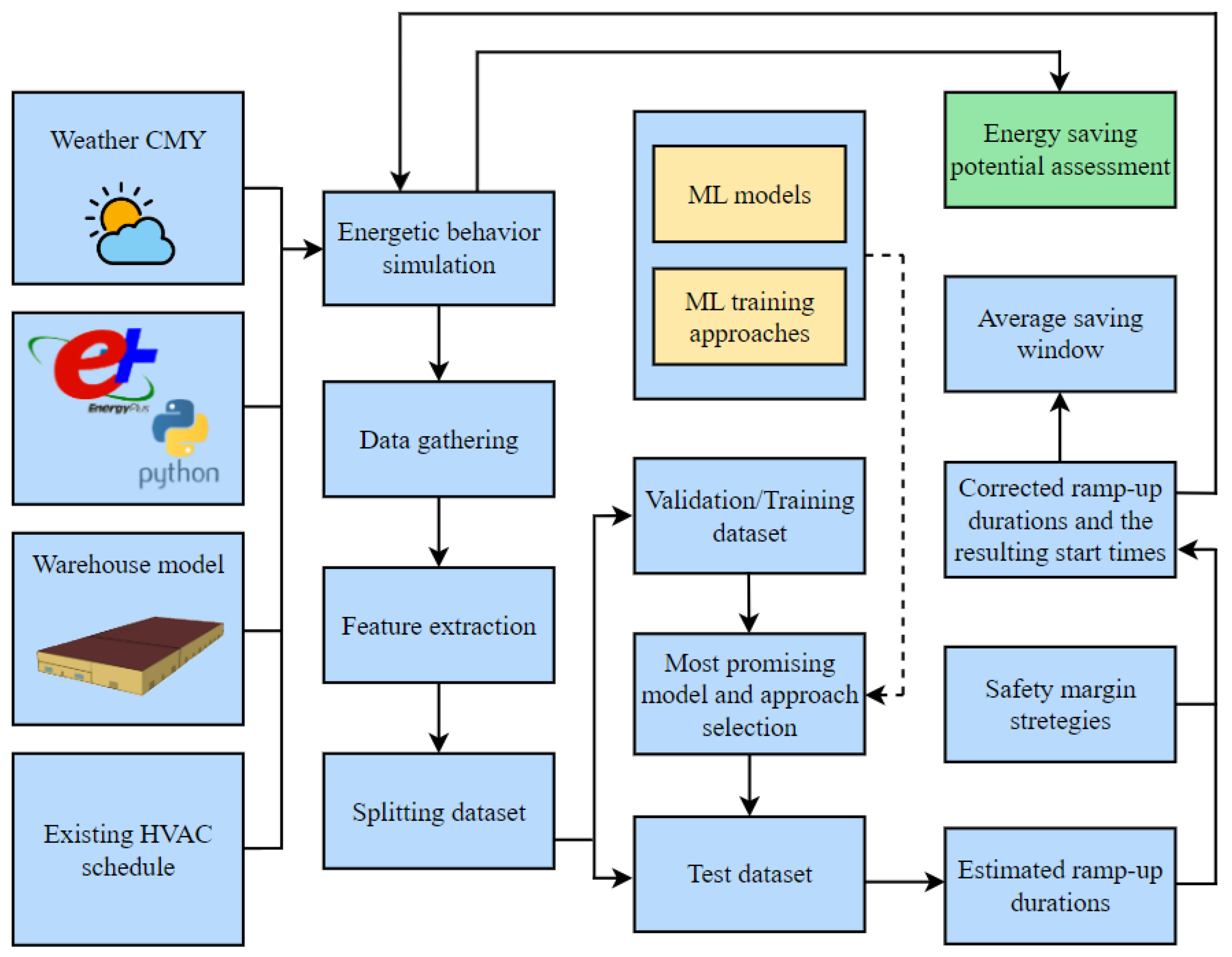
This section outlines the detailed methodology of the predictive modeling of morning ramp-up to improve energy performance in a warehouse building in Bologna, Italy. First, the physics-based simulation of the warehouse provides the energetic behavior of the different zones of the building. Next, machine learning pipelines with different training approaches (offline and sliding window) and state-of-the-art ML models are utilized to achieve the most accurate predictions for the duration of the morning ramp-ups. The average saving window using different safety margin scenarios is obtained, showing an opportunity for considerable energy savings in the building. Finally, to assess the energy-saving potential, the developed approach (adjusted daily heating start times based on ML predictions) is deployed on the warehouse zones using a re-simulation of the thermal behavior of the building. Furthermore,
Figure 1 presents a schematic representation of the adopted methodology.
2.1. Case Study
A physics-based co-simulation using EnergyPlus V9.4 [
19] and its Python API [
20] has been utilized in the current work. The reference warehouse building model is developed under the ANSI/ASHRAE/IES Standard 90.1 [
21] in Bologna, Italy. The example values of the parameters used in the warehouse physics-based modeling and simulation processes are provided in the
Appendix A. The energetic co-simulation considers the winter season heating scenario from November 2022 to April 2023 and provides data with a frequency of 60 timestamps per hour (1-min intervals), which is the maximum possible frequency to define in EnergyPlus, in order to increase the accuracy of the prediction of thermal behavior and its impact on energy consumption. The building model consists of two zones (office and storage) with different heating strategies. A detailed description of the building model and the simulation parameters are provided in
Table 1.
The default starting times for air conditioning in the office and storage areas are fixed and designed to meet user comfort requirements in the coldest days of the year, taking into account the capacity of the HVAC system designed for the space. Similar to the office zone, the storage zone is also utilized for peaking activities, which thus requires heating. In this work, a water-to-air heat pump is used as the heating source which is connected to the heating coil of an air handling unit (of a centralized air-based system) that is supplying warm air to the building. A water-to-air heat pump is an integrated system comprising a fan, water-to-air cooling and heating coils, and an auxiliary heating coil. This device transitions between cooling and heating modes based on the specific demands of the zone it serves. On the load side (air), it incorporates an on/off fan, a cooling coil, a heating coil, and a supplemental gas or electric heating coil. Conversely, the source side (water) connects to a condenser loop featuring a heat exchanger or a heating source, such as a boiler, and a cooling source, such as a chiller. This setup ensures efficient temperature regulation by transferring heat between water and air, tailored to the zone’s requirements [
19,
20]. An illustration of the connections between the heat pump’s source and load sides in a ground heat exchanger configuration can be found in EnergyPlus documentations [
20].
2.2. Physics-Based Energy Simulation and Extracting Ramp-Up Durations and Related Features
A standard methodology has been adopted to determine the durations of morning ramp-ups in the baseline scenario. As mentioned in
Table 1, the thermostats for office (zone 1) and storage (zone 2) are set to 21 °C and 19 °C, respectively, and these setpoint temperatures should be reached before or (in the worst case) on the arrival of the workers to the building in the morning. The working schedule of the zones for the working days (Monday until Friday) starts at 7 a.m. and lasts until 5 p.m. For technical reasons, such as reducing the risk of operation challenges, there is a setpoint temperature of 11 °C for heating during the unoccupied hours of weekdays and the whole period of weekends.
The physics-based simulation is conducted to extract the durations of morning ramp-ups, which is the time required by the heating system to raise the temperature of the zone from nighttime setback temperature to comfort temperature. It should be noted that in the baseline scenario, the starting time is fixed (default schedule of the building) and the duration of ramp-up varies based on indoor and outdoor conditions. For the office zone, the HVAC system is scheduled to start heating at 5:20, with a maximum ramp-up duration of 100 min in the worst-case scenario. On the other hand, despite the lower setpoint temperature of the storage zone, the heating system of the storage has to start earlier (at 4:04) than the office. The higher ramp-up duration of the storage (164 min in the worst-case scenario) is due to the significantly higher surface area of this zone.
Table 2 presents a summary of the weather conditions of the simulated warehouse model.
2.3. Feature Extraction Procedure
In supervised machine learning algorithms, features represent the input variables employed to train prediction models. An initial investigation is conducted to identify the key factors influencing the heating of the thermal zones. These factors include the heat input from the fan coil unit, the rate of thermal losses, and the thermal behavior of the zones. First, the identification process demonstrates that the time-series data of indoor temperature and its lagged values represent the thermal behavior of the zone and the rate of heat loss. These lagged values are included for up to 30 min before based on their importance in prediction, as determined through an initial feature correlation investigation. Subsequently, the outside temperature, a key factor affecting the required heating load, is included. Similarly, the lagged values of the outdoor temperature are incorporated to account for their delayed impact. Furthermore, since the developed pipelines estimate the duration of the ramp-up using input parameters available just before the ramp-up procedure begins, solar irradiation is excluded from the data. This exclusion is due to the fact that the sun does not rise before the ramp-up on most days and because of the delayed impact of solar radiation on indoor temperature. To account for the thermal interactions between zones and eliminate the need for detailed floor plan data, the mean temperature of building zones at the time of ramp-up is included in the dataset. This approach effectively captures the thermal influence of adjacent zones on each other. Lastly, to account for the thermal inertia of the zones, the temperature slopes over the last 15 and 30 min are included in the dataset. These slopes provide critical information about the rate of temperature change, reflecting the zones’ thermal response characteristics.
Table 3 provides the features extracted from the simulations to be utilized as input for training the ML models. The training dataset consists of these nine features as the input variables and the ramp-up duration as the target variable, with each day represented as a separate row in the dataset.
2.4. Machine Learning Modeling
The obtained dataset from the simulation contains the duration of the morning ramp-up and its corresponding features, which are mentioned in
Section 2.2, for each day. In this case, each row of the dataset contains the data regarding a day of the investigated period, and each row can be treated independently. The data set is divided using a random seed into a training/validation set and a test set with 80% and 20% share, respectively. In order to develop a generalized predictive model and prevent overfitting in the prediction procedure, k-fold cross-validation is used to partition the training/validation set into five folds, where each fold is an equal-sized data subset. In this way, four folds are used as training and one as a validation data subset, and the prediction error is calculated. This iterative process is repeated five times (k = 5), and the validation/training error is obtained as the average of these five iterations. Eventually, the trained model performs prediction on the test set, and the corresponding error is obtained. It should be noted that using a single random seed to split the dataset into training/validation and test sets can introduce biases. To prevent this potential issue, five different random seeds are used iteratively. The dataset is partitioned into a unique training/validation and test subset for each seed, allowing the models to be trained and tested on five different datasets. This process ensures a more reliable evaluation by providing an average test accuracy across multiple datasets.
In this work, to find the most accurate model for predicting the ramp-up duration, six different machine learning algorithms, including linear regression, Random Forest (RF), XGBoost, Extra Trees (ETs), Support Vector Machine (SVM), and K Nearest Neighbors (KNN), using offline and sliding window training approaches are employed, and their performances are compared. Finally, the accuracy for each model, considering both validation and testing datasets, is demonstrated using two accuracy metrics: Mean Absolute Error (MAE) [min] and Mean Absolute Percentage Error (MAPE) [%].
2.5. Machine Learning Training Approaches
In this study, both offline and sliding window training approaches have been utilized. In offline learning, the entire dataset is utilized to train the predictive model in its entirety and is advantageous for its ease of implementation, in case the entire dataset is available upfront. However, a shortcoming of this training method is that the model is not updated when new data becomes available. As a result, it cannot retrain to incorporate changes in underlying patterns, potentially leading to outdated and less accurate predictions over time [
22].
On the other hand, sliding window approaches provide a dynamic solution for processing sequential data by focusing on a subset of recent observations or a ‘training window’. This training window moves along the data stream, utilizing the most recent data for iteratively retraining the models, capturing temporal dependencies, and updating the model. These methods are particularly valuable for real-time applications or scenarios with significant changes in the data over time. However, selecting an appropriate window size is crucial, as it requires balancing the need to capture sufficient context to maintain computational efficiency [
23].
The present work uses offline and online (sliding window) training approaches to obtain the most accurate pipeline for ramp-up duration estimation. Three different window sizes are tested for the sliding window approach, and the one that leads to the most accurate performance is decided. The trained and tested window sizes are 5, 10, and 15 days. Further improvements can be obtained by systematically optimizing the training size of the window [
24]. As mentioned before, the online (sliding window) approach can significantly reduce the computational cost and make the pipeline less dependent on data availability.
3. Complementary Concepts
This section provides an overview of the concepts used in this study, including six different machine learning regression algorithms and two evaluation metrics employed to assess the accuracy and reliability of the ML models. The models employed in this research were sourced from the Python libraries Scikitlearn [
25] and XGBoost [
26].
3.1. Machine Learning Regression Algorithms
The algorithms chosen for this study are selected to represent a diverse array of machine learning categories and families. This selection is based on the proven effectiveness of these algorithms in the context of predicting the thermal behavior within building systems, using the results of a previous study (Alawadi et al. [
27] dedicated to comparing the performance of different ML algorithms in this area, along with the results obtained by the authors in their previous works ([
28,
29]). Simpler models, such as linear regression and k-nearest neighbors, are included to provide a baseline, taking into account their straightforward implementation. More advanced models are chosen for their ability to handle non-linear relationships, manage high-dimensional data, maintain robustness against overfitting, and the capability of performing well while being trained with small to medium-sized datasets. These characteristics ensure that the chosen algorithms can effectively address the complexities and nuances inherent in predicting heating duration in buildings.
3.1.1. Linear Regression (LR)
Linear regression is a fundamental statistical method used to model and analyze the relationship between a dependent variable and one or more independent variables. Linear regression aims to establish a linear equation that predicts the dependent variable based on the independent variables by minimizing the residual sum of squares, thereby quantifying the difference between the observed data and the predicted values [
30]. This method assumes a linear relationship between the variables, which is mathematically represented as Equation (
1):
The equation features a dependent variable, y, as well as independent variables, , , …, , and coefficients, , , , …, .
3.1.2. Random Forest Regressor (RFR)
The Random Forest Regressor (RFR) is a machine-learning algorithm that operates by constructing multiple decision trees during training. Each tree is trained on a random subset of the data and a random subset of the features. Predictions are made by averaging the outputs of all the individual trees, which helps reduce overfitting and improves generalization. RFR is particularly well-suited for datasets with complex relationships and high-dimensional spaces [
31].
3.1.3. Extra Tree Regressor (ETR)
The Extra Tree Regressor (ETR) is a machine learning algorithm that belongs to the ensemble learning family, similar to random forest. It builds multiple decision trees using random subsets of the training data and averages the predictions from these trees to enhance robustness and accuracy [
32]. The level of randomness introduced in the split selection process distinguishes Extremely Randomized Trees (ETs) from random forests. While random forests search for the best possible thresholds to split each node, Extremely randomized trees choose random thresholds for each feature. This increased randomness helps to reduce variance and can lead to faster training times compared to random forests [
33].
3.1.4. XGBoost Regressor (XGBR)
Similar to the random forest and extra trees, XGBoost (Extreme Gradient Boosting) is also a powerful tree-based machine learning algorithm, but it enhances performance by using gradient boosting. It builds and trains weak decision trees sequentially, each time utilizing the errors from previous iterations to improve the subsequent tree’s performance. This iterative process allows XGBoost to effectively minimize the overall error of the model, leading to high prediction accuracy [
26].
3.1.5. K Nearest Neighbors Regressor (KNNR)
The K Nearest Neighbors (KNN) regressor is a non-parametric algorithm used for regression tasks in machine learning, which operates on the principle that similar data points should have similar output values. In KNN regression, predictions are made by averaging the target values of the k-nearest neighbors in the training set [
34]. The choice of k (the number of neighbors) is crucial as it influences the smoothness and accuracy of the model’s predictions. Smaller values of k lead to more complex models with potentially high variance (overfitting), whereas larger values of k result in smoother predictions that may introduce bias (underfitting). The proper selection of k is essential for balancing the trade-off between bias and variance to achieve optimal model performance [
35].
3.1.6. Support Vector Regressor (SVR)
The Support Vector Regressor (SVR) is a type of Support Vector Machine (SVM) designed specifically for regression tasks. In contrast to traditional linear regression models, which aim to minimize the error between predicted and actual values, SVR seeks to find a function that approximates the data within a specified tolerance margin [
36]. This approach involves fitting the best line (or hyperplane in higher dimensions) within a threshold defined by the parameter epsilon (
), which sets the width of the acceptable deviation from the regression line [
37].
3.2. Evaluation Metrics
3.2.1. Mean Absolute Error (MAE)
The Mean Absolute Error (MAE) given by Equation (
2) is a metric used to evaluate the accuracy of a predictive model by calculating the average absolute differences between predicted and actual values. It provides a straightforward measure of error magnitude, unaffected by the direction of deviations, making it easy to interpret.
3.2.2. Mean Absolute Percentage Error (MAPE)
The Mean Absolute Percentage Error (MAPE) given by Equation (
3) is a statistical measure that quantifies the average absolute deviation error expressed as a percentage, allowing for a straightforward comparison between different prediction models.
In these equations, presents the actual value of the i-th element in the dataset, shows the predicted value of the i-th element in the dataset, i denotes the index of the elements in the dataset, and n represents the total number of elements in the dataset.
4. Results and Discussion
This section initially presents the results of the physics-based simulation and investigation of the warehouse’s thermal behavior. For each zone of the building, the ramp-up durations and the required weather-based data were extracted. Next, various ML-based pipelines, utilizing different models and training approaches, were implemented to identify the most effective one for predicting ramp-up durations in each warehouse zone. MAPE and MAE metrics were used to evaluate the performance of the predictive models. The best machine learning pipelines were then selected for each zone based on the obtained test results, and two different strategies (conservative and semi-conservative saving) were proposed to investigate the values of the average saving window. The average saving window (minutes per day) would be the average of the difference between the existing heating initiation schedule and the starting time obtained using the ML models. This would indirectly evaluate the possible potential of energy saving. Finally, another physics-based simulation was conducted after deploying the developed approach, and the energy-saving potential (kWh per year) was assessed.
4.1. Energetic Behaviour Simulation
This subsection provides the results of the energetic behavior simulations explained in
Section 2.2. In the default HVAC schedule of the buildings, setpoints were adjusted for zone 1 (office) at 5:20 and for zone 2 (storage) at 4:04 in order to ensure thermal comfort in the morning for users (based on the longest ramp-up duration required throughout the year). Due to continuous fluctuations in indoor and outdoor temperatures, as well as the performance of the designed heating system, the ramp-up duration was observed to change consistently from day to day.
Figure 2 presents an example of the morning ramp-up in the physics-based simulated model on a day with moderate environmental conditions, while the outside temperature is around 8 °C when the setpoint temperature increases in the morning. In this case, the office and storage experience ramp-up durations of 32 and 68 min, respectively. This thermal behavior demonstrates significant energy-saving potential on this day, as the heating setpoint temperature is achieved more than an hour before workers enter each zone of the warehouse.
On the other hand,
Figure 3 shows the simulated morning ramp-up behavior in extreme environmental conditions. On this specific day, the outside temperature of the building decreases to values below 0 °C when the heating starts in the zones. As a result, the ramp-up durations of the office and storage are significantly higher than the previous example, with 83 and 131 min, respectively.
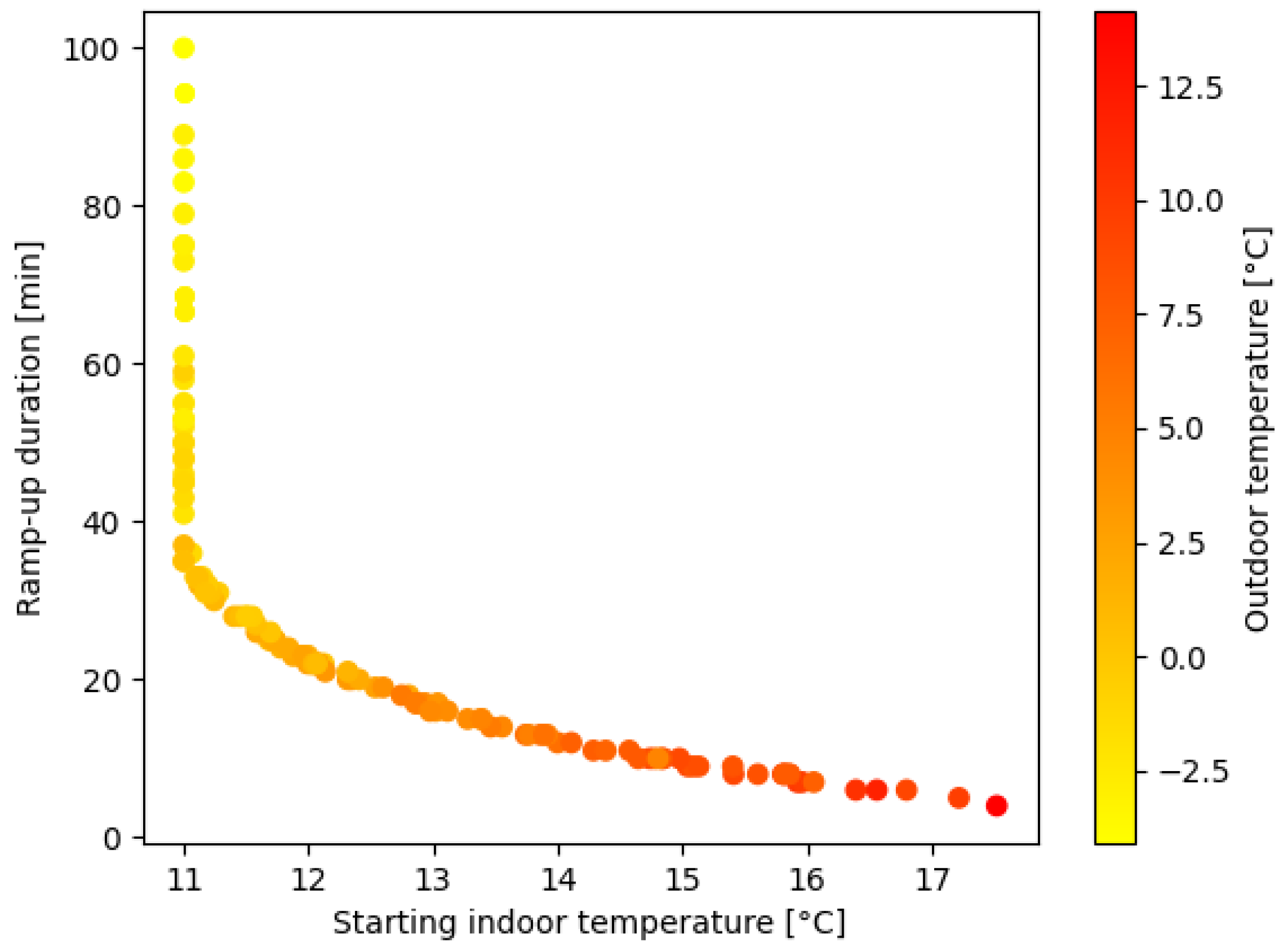
A broader analysis of the physics-based simulated morning ramp-up event reveals a dynamic behavior with a wide range of ramp-up duration values over the heating season. It can be observed that the ramp-up duration varies daily and differs between zones on the same day.
Figure 4 and
Figure 5 illustrate that these ramp-up durations are highly negatively correlated with both indoor and outdoor temperatures when the heating setpoint temperature rises in the morning.
4.2. Predictive Modeling
The following subsections present the results and discussion regarding the accuracy of the predictive models in forecasting the morning ramp-up durations for each zone of the physics-based simulated warehouse. Regarding the methodology detailed in
Section 2.4 and
Section 2.5, the performance of six different ML models is compared using offline and sliding window training approaches for zones 1 (office) and 2 (storage). This separate comparison is due to their differing heating setpoint temperatures and HVAC system start times. The reliability of the models is assessed using k-fold cross-validation. To ensure the reliability of the obtained results, the entire training/validation and testing process is repeated five times with different train/validation and test subsets created using five randomly generated seeds. As a result, the reported final values represent averages across all seeds and the corresponding standard deviations.
4.2.1. Zone 1—Office
Table 4 reports the performance of the ML learning models for zone 1 (office) on the training/validation dataset. The results indicate that using the offline training approach, tree-based ensemble algorithms perform the best, with the random forest algorithm achieving the lowest MAPE of 12.95%.
Therefore, selecting the random forest algorithm, its performance has been evaluated on the test set (
Table 5) leading to an MAE of 3 min, illustrating its reliability. Since the sliding window training approach does not improve the model performance, the corresponding results are not included.
4.2.2. Zone 2—Storage
As presented in
Table 6, similar to zone 1 (office), the performances of tree-based ensemble models are more accurate compared to other algorithms for zone 2 (storage). In this zone, the sliding window training approach resulted in more reliable predictions than the offline training approach, and the performances of the machine learning models are obtained by employing three different window sizes: 5, 10, and 15 days. Increasing the window size from 5 to 10 days improved the model’s accuracy, while further increasing it to 15 days yielded similar accuracy values. Since the predictive model’s performance did not improve beyond a 10-day window, further increases in window length were not pursued. Thus, a 15-day window was selected as the optimal size for prediction. The best result on the training/validation set was obtained using the Extra Trees (ETs) model, with a Mean Absolute Percentage Error (MAPE) of 16.5%.
Table 7 presents the performance of the Extra Trees (ETs) machine learning algorithm using the sliding window training approach on the test dataset, yielding an MAE of 3 min, consistent with the results for the office zone.
4.2.3. Discussions on Performance of ML Algorithms
Linear regression algorithm has been observed to exhibit the poorest performance among the algorithms due to its inability to capture the non-linear relationships inherent in the dataset. The duration of the heating ramp-up is influenced by the thermal behavior of the building, which is implicitly represented by the input features. Linear regression’s linear assumptions fail to accommodate these complex, non-linear dynamics effectively. Similarly, k-Nearest Neighbors (k-NN) and Support Vector Regression (SVR) also struggle with this dataset, primarily due to challenges associated with high dimensionality. In contrast, tree-based algorithms demonstrate superior performance in this application. Their success can be attributed to their ability to capture non-linear relationships between features effectively. Their robustness to outliers and overfitting enhances their accuracy and generalization, making them ideal for predicting the ramp-up duration in the context of the current work.
4.3. Saving Potential Assessment
The current section initially provides the results of calculating the two safety margin strategies proposed to guarantee the thermal comfort of the occupants. Next, the saving window obtained using these safety margins is investigated. Finally, the potential energy savings that can be achieved in case the obtained predictive models are deployed in the physics-based simulated warehouse are provided.
Two different strategies (conservative and semi-conservative) are defined to calculate the safety margin values in the present work. The conservative strategy considers all the underestimations (differences between the estimated optimal morning ramp-up durations and the actual values), selects the biggest value, and adds it to the prediction of the model to ensure that the value of the ramp-up is not underpredicted. On the other hand, using the semi-conservative approach, the outlier threshold is set at 10%, meaning the top 10% of underestimated values are excluded from the safety margin calculation. Adopting a semi-conservative strategy can be more realistic, as it excludes extreme underestimations. The conservative strategy requires safety margin values of 20 and 44 min for the office and storage zone, respectively, while these values using the semi-conservative strategy are equal to 4 and 6 min. Next, the saving windows (the time that heating can be avoided in a zone using the proposed predictive approach compared to the default HVAC schedule) can be calculated for each day of each zone. The results are presented in
Table 8, demonstrating substantial average savings across all zones and scenarios and emphasizing the immense energy-saving potential of deploying the smart morning ramp-up system in the building.
As mentioned in
Section 2, to assess the energy-saving potential, the optimal starting times of the heating system are deployed in the reference warehouse. As a result, a physics-based resimulation is performed to evaluate the energy performance of the smart building, and the results are compared to the baseline thermal simulation model. The comparison shows a notable potential for energy savings, with the conservative strategy achieving a 10.13% reduction and the semi-conservative strategy achieving an 8.23% reduction for the entire building.
Table 9 presents the energy consumption and saving values for each zone and the entire warehouse using different strategies, highlighting that the storage zone has the highest energy consumption and the greatest potential for energy savings. Furthermore, the substantial savings achieved for the entire building demonstrate the effectiveness of the proposed approach in reducing energy consumption and enhancing efficiency in warehouses.
5. Conclusions
This study proposed a machine learning-based solution attempting to enhance the energy efficiency of HVAC systems in logistic nodes and warehouse buildings with nighttime setback schedules. The case study of a warehouse building in Bologna, Italy, was investigated to assess the energy-saving potential of an ML-based approach for estimating the optimal daily heating start times for each zone whilst ensuring that the thermal comfort of the building is respected. By estimating the time required for the heating system to heat up the zone to the comfort temperature, rather than using fixed starting times, heating unoccupied zones is avoided, resulting in significant energy savings. Physics-based energy simulations (using the EnergyPlus 9.4 software) were conducted to model the energetic behavior of the warehouse. The simulated time-series data of indoor temperature, setpoints, and other related features were collected in addition to the corresponding weather data to capture the thermal behavior of the zones, the influence of the HVAC system, and the rate of thermal losses to the environment. Next, these data were employed to train ML models to predict the duration of the ramp-up for each zone of the building.
Six different ML regressor models were considered and trained to predict the ramp-up duration of different zones during the mornings of winter 2022–2023. The selected ML algorithms were linear regressor, extra trees regressor, random forest regressor, XGBoost, support vector regressor, and k-nearest neighbors. Their offline performances (using the whole data) were compared to a sliding window-based training approach. The accuracies were evaluated in terms of MAE and MAPE. It was found that random forest in the offline training approach provides the most accurate pipeline for the office (MAE of 3 min and MAPE of 12.76%), the extra trees model with the online (sliding window) approach is best for the storage zone (MAE of 3 min and MAPE of 15.84%).
Next, considering the maximum underestimation error made by the error, the two safety margin scenarios were proposed, ensuring the comfort of the occupants would not be compromised. Therefore, in the conservative method, the largest underestimation from the model predictions was added to the model’s forecast, while the semi-conservative approach dropped the top 10% of underestimation (outliers) before calculating the safety margin. Next, the saving average window (the difference between the heating initiation time proposed with this approach and the default schedule of the building) was calculated for each zone using conservative and semi-conservative approaches. The obtained results showed that there was a considerable potential for energy saving for the case study.
Lastly, in order to assess the energy-saving potential of the proposed approach, in case it is deployed in the building, a physics-based resimulation of the warehouse was performed, and the energy performance of the building equipped with smart morning ramp-up systems was assessed. Obtained results indicated that a significant energy saving could be obtained, achieving 8.23% and 10.13% of total building energy savings using conservative and semi-conservative strategies, respectively. It can be concluded that the proposed approach offers a significant potential for energy saving and is suitable for deployment in conditioned warehouses. Additionally, in the context of the current work, no data regarding the size of the buildings or details of the floor plan has been included to enhance the generalizability of this study. Therefore, the proposed method can be deployed in already existing warehouse buildings with building management systems. Consequently, given the substantial savings demonstrated by the proposed methodology in this study, the deployment of such an approach can be proposed as future work in real case study logistic nodes to achieve energy efficiency and validate the obtained results.
Author Contributions
A.K.: software, formal analysis, validation, investigation, data curation, writing—original draft; F.D.J.: formal analysis, methodology, validation, data curation, writing—original draft; I.A.C.A.: software, formal analysis, validation; B.N.: conceptualization, methodology, supervision, writing—review and editing; L.P.M.C.: supervision, methodology; S.P.: writing—review and editing, supervision; F.R.: supervision, funding acquisition. All authors have read and agreed to the published version of the manuscript.
Funding
This research is part of a broader project financed by the European Union NextGenerationEU (National Sustainable Mobility Center CN00000023, Italian Ministry of University and Research Decree n. 1033—17 June 2022, Spoke 10 “Sustainable Logistics”).
Data Availability Statement
The original contributions presented in the study are included in the article, further inquiries can be directed to the corresponding author.
Conflicts of Interest
The authors declare no conflict of interest.
Appendix A. Example Parameters for Warehouse Modeling and Simulations
Table A1.
Zone summary.
| | Area | Volume | Gross Wall Area | Window Glass Area | Opening Area | Lighting | Plug and Process |
|---|
| |
[m2]
|
[m3]
|
[m2]
|
[m2]
|
[m2]
|
[W/m2]
|
[W/m2]
|
|---|
| Zone 1 (Office) | 236.9 | 1010.8 | 149.6 | 17.7 | 17.7 | 6.89 | 8.07 |
| Zone 2 (Fine Storage) | 4598.2 | 38,230.6 | 2347.4 | 0.0 | 0.0 | 3.55 | 1.78 |
| Total | 4835.1 | 39,241.4 | 2497.0 | 17.7 | 17.7 | 3.72 | 2.09 |
Table A2.
Opaque exterior.
Table A2.
Opaque exterior.
| | Reflectance | U-Factor with Film | U-Factor No Film | Gross Area | Net Area | Azimuth | Tilt | Cardinal Direction |
|---|
| | |
[W/m2-K]
|
[W/m2-K]
|
[m2]
|
[m2]
|
[deg]
|
[deg]
| |
|---|
| Office (front wall) | 0.30 | 0.528 | 0.573 | 110.5 | 97.4 | 270 | 90 | W |
| Office (left wall) | 0.30 | 0.528 | 0.573 | 39.0 | 30.6 | 0 | 90 | N |
| Office (floor) | 1.00 | 0.187 | 0.193 | 236.9 | 236.9 | 90 | 180 | - |
| Fine Storage (front wall) | 0.30 | 0.528 | 0.573 | 169.1 | 161.6 | 270 | 90 | W |
| Fine Storage (right wall) | 0.30 | 0.528 | 0.573 | 260.1 | 243.3 | 180 | 90 | S |
| Fine Storage (left wall) | 0.30 | 0.528 | 0.573 | 182.1 | 172.7 | 0 | 90 | N |
| Office (front wall) | 0.30 | 0.528 | 0.573 | 110.5 | 110.5 | 270 | 90 | W |
| Fine Storage (office left wall) | 0.30 | 0.528 | 0.573 | 39.0 | 39.0 | 0 | 90 | N |
| Fine Storage (floor) | 1.00 | 0.166 | 0.171 | 1156.5 | 1156.5 | 90 | 180 | - |
| Fine Storage (roof) | 0.23 | 0.233 | 0.240 | 1393.4 | 1372.6 | 90 | 0 | - |
Table A3.
Opaque interior.
Table A3.
Opaque interior.
| | Reflectance | U-Factor with Film | U-Factor No Film | Gross Area | Net Area | Azimuth | Tilt | Cardinal Direction |
|---|
| | |
[W/m2-K]
|
[W/m2-K]
|
[m2]
|
[m2]
|
[deg]
|
[deg]
| |
|---|
| Office right wall | 0.30 | 0.653 | 0.775 | 39.0 | 39.0 | 180 | 90 | S |
| Office rear wall | 0.30 | 0.653 | 0.775 | 110.5 | 110.5 | 90 | 90 | E |
| Office roof | 0.30 | 2.711 | 10.063 | 236.9 | 236.9 | 90 | 0 | - |
| iz-Office right wall * | 0.30 | 0.653 | 0.775 | 39.0 | 39.0 | 0 | 90 | N |
| iz-Office rear wall * | 0.30 | 0.653 | 0.775 | 110.5 | 110.5 | 270 | 90 | W |
| iz-Office roof * | 0.30 | 2.711 | 10.063 | 236.9 | 236.9 | 270 | 180 | - |
Table A4.
Exterior fenestration.
Table A4.
Exterior fenestration.
| | Glass Area | Glass U-Factor | Glass SHGC | Glass Visible Transmittance | Azimuth | Tilt | Cardinal Direction |
|---|
| |
[m2]
|
[W/m2-K]
| | |
[deg]
|
[deg]
| |
|---|
| Office front wall window 1 | 5.58 | 2.843 | 0.231 | 0.231 | 270 | 90 | W |
| Office front wall window 2 | 5.58 | 2.843 | 0.231 | 0.231 | 270 | 90 | W |
| Office left wall window 1 | 3.25 | 2.843 | 0.231 | 0.231 | 0 | 90 | N |
| Office left wall window 2 | 3.25 | 2.843 | 0.231 | 0.231 | 0 | 90 | N |
| Fine Storage Skylight 1 | 1.49 | 3.979 | 0.303 | 0.301 | 180 | 0 | - |
| Fine Storage Skylight 2 | 1.49 | 3.979 | 0.303 | 0.301 | 180 | 0 | - |
| Fine Storage Skylight 3 | 1.49 | 3.979 | 0.303 | 0.301 | 180 | 0 | - |
| Fine Storage Skylight 4 | 1.49 | 3.979 | 0.303 | 0.301 | 180 | 0 | - |
| Fine Storage Skylight 5 | 1.49 | 3.979 | 0.303 | 0.301 | 180 | 0 | - |
| Fine Storage Skylight 6 | 1.49 | 3.979 | 0.303 | 0.301 | 180 | 0 | - |
| Fine Storage Skylight 7 | 1.49 | 3.979 | 0.303 | 0.301 | 180 | 0 | - |
| Fine Storage Skylight 8 | 1.49 | 3.979 | 0.303 | 0.301 | 180 | 0 | - |
| Fine Storage Skylight 9 | 1.49 | 3.979 | 0.303 | 0.301 | 180 | 0 | - |
| Fine Storage Skylight 10 | 1.49 | 3.979 | 0.303 | 0.301 | 180 | 0 | - |
| Fine Storage Skylight 11 | 1.49 | 3.979 | 0.303 | 0.301 | 180 | 0 | - |
| Fine Storage Skylight 12 | 1.49 | 3.979 | 0.303 | 0.301 | 180 | 0 | - |
| Fine Storage Skylight 13 | 1.49 | 3.979 | 0.303 | 0.301 | 180 | 0 | - |
| Fine Storage Skylight 14 | 1.49 | 3.979 | 0.303 | 0.301 | 180 | 0 | - |
Table A5.
Exterior door.
| | U-Factor with Film | U-Factor No Film | Gross Area | Parent Surface |
|---|
| |
[W/m2-K]
|
[W/m2-K]
|
[m2]
| |
|---|
| Office front door | 1.599 | 2.102 | 1.95 | Office front wall |
| Office left wall door | 1.599 | 2.102 | 1.95 | Office left wall |
| Fine Storage overhead door 1 | 1.394 | 1.761 | 7.43 | Fine Storage front wall |
| Fine Storage overhead door 2 | 1.394 | 1.761 | 7.43 | Fine Storage right wall |
| Fine Storage overhead door 3 | 1.394 | 1.761 | 7.43 | Fine Storage right wall |
| Fine Storage overhead door 4 | 1.394 | 1.761 | 7.43 | Fine Storage left wall |
| Fine Storage right door | 1.599 | 2.102 | 1.95 | Fine Storage right wall |
| Fine Storage left door | 1.599 | 2.102 | 1.95 | Fine Storage left wall |
Table A6.
Interior lighting.
Table A6.
Interior lighting.
| | Lighting Power Density | Zone Area | Total Power | Scheduled Hours/Week | Hours/Week > 1% | Full Load Hours/Week | Consumption |
|---|
| |
[W/m2]
|
[m2]
|
[W]
|
[h]
|
[h]
|
[h]
|
[GJ]
|
|---|
| Office lights | 6.89 | 236.88 | 1631.84 | 56.99 | 168 | 39.73 | 5.03 |
| Fine Storage lights | 3.55 | 4598.25 | 16,333.41 | 62.12 | 168 | 47.01 | 59.63 |
Table A7.
Daylighting.
| | Fraction Controlled | Lighting Installed | Lighting Controlled |
|---|
| | |
[W]
|
[W]
|
|---|
| Office Daylighting 1 | 0.29 | 1631.84 | 473.23 |
| Office Daylighting 2 | 0.10 | 1631.84 | 163.18 |
| Fine Storage Daylighting 1 | 0.25 | 16,333.41 | 4083.35 |
| Fine Storage Daylighting 2 | 0.25 | 16,333.41 | 4083.35 |
Table A8.
Exterior lighting.
Table A8.
Exterior lighting.
| | Total Watts | Hours/Week > 1% | Full Load Hours/Week | Consumption |
|---|
| | [W] | [h] | [h] | [GJ] |
| Exterior lights A | 113.8 | 57.12 | 57.12 | 0.50 |
| Exterior lights B | 3955.0 | 99.12 | 78.12 | 23.99 |
| Exterior lights C | 1004.9 | 99.12 | 64.12 | 5.00 |
References
- Navickas, V.; Sujeta, L.; Vojtovich, S. Logistics systems as a factor of country’s competitiveness. Econ. Manag. 2011, 16, 231–237. [Google Scholar]
- Li, X.; Sohail, S.; Majeed, M.T.; Ahmad, W. Green logistics, economic growth, and environmental quality: Evidence from one belt and road initiative economies. Environ. Sci. Pollut. Res. 2021, 28, 30664–30674. [Google Scholar] [CrossRef]
- Piecyk, M.I.; McKinnon, A.C. Forecasting the carbon footprint of road freight transport in 2020. Int. J. Prod. Econ. 2010, 128, 31–42. [Google Scholar] [CrossRef]
- Fichtinger, J.; Ries, J.M.; Grosse, E.H.; Baker, P. Assessing the environmental impact of integrated inventory and warehouse management. Int. J. Prod. Econ. 2015, 170, 717–729. [Google Scholar] [CrossRef]
- Ries, J.M.; Grosse, E.H.; Fichtinger, J. Environmental impact of warehousing: A scenario analysis for the United States. Int. J. Prod. Res. 2017, 55, 6485–6499. [Google Scholar] [CrossRef]
- Dadras Javan, F.; Campodonico Avendano, I.A.; Najafi, B.; Moazami, A.; Rinaldi, F. Machine-learning-based prediction of hvac-driven load flexibility in warehouses. Energies 2023, 16, 5407. [Google Scholar] [CrossRef]
- REZNOR HVAC. Efficient Warehouse Heating, Cooling & Ventilation Tips. Available online: https://www.reznorhvac.com/efficient-warehouse-heating-cooling-ventilation-tips (accessed on 7 June 2024).
- Nweye, K.; Nagy, Z. MARTINI: Smart meter driven estimation of HVAC schedules and energy savings based on Wi-Fi sensing and clustering. Appl. Energy 2022, 316, 118980. [Google Scholar] [CrossRef]
- Gunay, H.B.; O’Brien, W.; Beausoleil-Morrison, I.; Bursill, J. Implementation of an Adaptive Occupancy and Building Learning Temperature Setback Algorithm. Ashrae Trans. 2016, 122, 179. [Google Scholar]
- Gao, G.; Whitehouse, K. The self-programming thermostat: Optimizing setback schedules based on home occupancy patterns. In Proceedings of the First ACM Workshop on Embedded Sensing Systems for Energy-Efficiency in Buildings, Berkeley, CA, USA, 3 November 2009; pp. 67–72. [Google Scholar]
- Seem, J.E.; House, J.M.; Alcala, C.F. Model Selection for Predicting the Return Time from Night Setback. In Proceedings of the 4th International High Performance Buildings Conference at Purdue 2016, West Lafayette, IN, USA, 11–14 July 2016. [Google Scholar]
- Wu, C.; Chen, Z.; Zhang, Y.; Feng, J.; Xie, Y.; Qin, C. A case study of multi-energy complementary systems for the building based on Modelica simulations. Energy Convers. Manag. 2024, 306, 118290. [Google Scholar] [CrossRef]
- Kossel, R.; Tegethoff, W.; Bodmann, M.; Lemke, N. Simulation of complex systems using Modelica and tool coupling. In Proceedings of the 5th Modelica Conference, Vienna, Austria, 4–5 September 2006; Volume 2, pp. 485–490. [Google Scholar]
- Amasyali, K.; El-Gohary, N.M. Real data-driven occupant-behavior optimization for reduced energy consumption and improved comfort. Appl. Energy 2021, 302, 117276. [Google Scholar] [CrossRef]
- Yang, I.H.; Yeo, M.S.; Kim, K.W. Application of artificial neural network to predict the optimal start time for heating system in building. Energy Convers. Manag. 2003, 44, 2791–2809. [Google Scholar] [CrossRef]
- Moon, J.W.; Jung, S.K. Algorithm for optimal application of the setback moment in the heating season using an artificial neural network model. Energy Build. 2016, 127, 859–869. [Google Scholar] [CrossRef]
- Moon, J.W.; Yoon, Y.; Jeon, Y.H.; Kim, S. Prediction models and control algorithms for predictive applications of setback temperature in cooling systems. Appl. Therm. Eng. 2017, 113, 1290–1302. [Google Scholar] [CrossRef]
- Dadras Javan, F.; Campodonico Avendano, I.A.; Najafi, B.; Rossi, M.; Rinaldi, F. Estimating morning ramp-up duration for the cooling season in a smart building using machine learning: Determining most promising features. Sustain. Energy Technol. Assess. 2024, 69, 103911. [Google Scholar] [CrossRef]
- Crawley, D.B.; Lawrie, L.K.; Winkelmann, F.C.; Buhl, W.F.; Huang, Y.J.; Pedersen, C.O.; Strand, R.K.; Liesen, R.J.; Fisher, D.E.; Witte, M.J.; et al. EnergyPlus: Creating a new-generation building energy simulation program. Energy Build. 2001, 33, 319–331. [Google Scholar] [CrossRef]
- Input Output Reference. EnergyPlus Version 9.6.0 Documentation, Tech. rep., U.S. Department of Energy. 2021. Available online: https://energyplus.net/assets/nrel_custom/pdfs/pdfs_v9.6.0/InputOutputReference.pdf (accessed on 1 July 2024).
- ANSE/ASHRAE/IES Standard 90.1-2010; Energy Standard for Buildings Except Low Rise Residential Buildings. ASHRAE: Atlanta, GA, USA, 2010.
- Bishop, C.M. Pattern Recognition and Machine Learning; Springer: New York, NY, USA, 2006. [Google Scholar]
- Gama, J.; Gaber, M.M. Learning from Data Streams: Processing Techniques in Sensor Networks; Springer: Berlin/Heidelberg, Germany, 2007. [Google Scholar]
- Mohsen, O.; Petre, C.; Mohamed, Y. Machine-learning approach to predict total fabrication duration of industrial pipe spools. J. Constr. Eng. Manag. 2023, 149, 04022172. [Google Scholar] [CrossRef]
- Pedregosa, F.; Varoquaux, G.; Gramfort, A.; Michel, V.; Thirion, B.; Grisel, O.; Blondel, M.; Prettenhofer, P.; Weiss, R.; Dubourg, V.; et al. Scikit-learn: Machine Learning in Python. J. Mach. Learn. Res. 2011, 12, 2825–2830. [Google Scholar]
- Chen, T.; Guestrin, C. XGBoost: A Scalable Tree Boosting System. In Proceedings of the 22nd ACM SIGKDD International Conference on Knowledge Discovery and Data Mining, San Francisco, CA, USA, 13–17 August 2016; ACM: New York, NY, USA, 2016; pp. 785–794. [Google Scholar] [CrossRef]
- Alawadi, S.; Mera, D.; Fernández-Delgado, M.; Alkhabbas, F.; Olsson, C.M.; Davidsson, P. A comparison of machine learning algorithms for forecasting indoor temperature in smart buildings. Energy Syst. 2020, 13, 689–705. [Google Scholar] [CrossRef]
- Papadopoulos, D.N.; Javan, F.D.; Najafi, B.; Mamaghani, A.H.; Rinaldi, F. Handling complete short-term data logging failure in smart buildings: Machine learning based forecasting pipelines with sliding-window training scheme. Energy Build. 2023, 301, 113694. [Google Scholar] [CrossRef]
- Javan, F.D.; Avendano, I.A.C.; Kaboli, A.; Najafi, B.; Moazami, A.; Perotti, S.; Rinaldi, F. Electricity demand flexibility estimation in warehouses using machine learning. In Big Data Application in Power Systems; Elsevier: Amsterdam, The Netherlands, 2024; pp. 323–348. [Google Scholar]
- Su, X.; Yan, X.; Tsai, C. Linear regression. Wiley Interdiscip. Rev. Comput. Stat. 2012, 4, 275–294. [Google Scholar] [CrossRef]
- Breiman, L. Random Forests. Mach. Learn. 2001, 45, 5–32. [Google Scholar] [CrossRef]
- Geurts, P.; Ernst, D.; Wehenkel, L. Extremely Randomized Trees. Mach. Learn. 2006, 63, 3–42. [Google Scholar] [CrossRef]
- Aziz, T.; Camana, M.; García, C.; Hwang, T.; Koo, I. REM-Based Indoor Localization with an Extra-Trees Regressor. Electronics 2023, 12, 4350. [Google Scholar] [CrossRef]
- Cover, T.; Hart, P. Nearest neighbor pattern classification. IEEE Trans. Inf. Theory 1967, 13, 21–27. [Google Scholar] [CrossRef]
- Hastie, T.; Tibshirani, R.; Friedman, J. The Elements of Statistical Learning: Data Mining, Inference, and Prediction, 2nd ed.; Springer Series in Statistics; Springer: New York, NY, USA, 2009. [Google Scholar]
- Smola, A.; Schölkopf, B. A tutorial on support vector regression. Stat. Comput. 2004, 14, 199–222. [Google Scholar] [CrossRef]
- Khanna, R.; Awad, M. Efficient Learning Machines: Theories, Concepts, and Applications for Engineers and System Designers; Springer Nature: Berlin, Germany, 2015. [Google Scholar] [CrossRef]
| Disclaimer/Publisher’s Note: The statements, opinions and data contained in all publications are solely those of the individual author(s) and contributor(s) and not of MDPI and/or the editor(s). MDPI and/or the editor(s) disclaim responsibility for any injury to people or property resulting from any ideas, methods, instructions or products referred to in the content. |
© 2024 by the authors. Licensee MDPI, Basel, Switzerland. This article is an open access article distributed under the terms and conditions of the Creative Commons Attribution (CC BY) license (https://creativecommons.org/licenses/by/4.0/).


 ,
, 

